

Submitted:
11 May 2026
Posted:
12 May 2026
You are already at the latest version
Abstract
Highway–rail grade crossing (HRGC) safety analysis is often based on raw incident counts or site-level models that do not control for exposure and ignore spatial dependence. This limits the ability to identify where risk is structurally concentrated across the rail network. The problem is important because misidentifying high-risk environments leads to inefficient allocation of limited safety resources and weakens corridor-level intervention strategies. This study introduces accumulated incidents per crossing (AIPX), an exposure-normalized metric that measured cumulative incident burden at the county level over a 51-year period (1975–2025). The study developed an algorithmic framework that integrates data reconciliation with spatial autocorrelation analysis, distributional modeling, and nonparametric machine learning to identify and interpret high-intensity risk environments. Global Moran’s I indicates statistically significant positive spatial autocorrelation (I = 0.359, p = 0.001), confirming that incident intensity is spatially clustered rather than random. Local indicators identify coherent high and low intensity county clusters. Distributional analysis shows that AIPX in high intensity clusters follows heavy-tailed behavior best represented by lognormal and Johnson SU distributions, indicating concentrated risk in a small subset of counties. Machine learning models achieve strong classification performance (AUC ≈ 0.85), with explainability methods consistently identifying temperature, train direction, crossing warning configuration, train composition, and track class as dominant associated features. These variables function as proxies for exposure intensity and network structure rather than causal drivers. The findings demonstrate that HRGC risk is a regional, network-driven phenomenon concentrated along freight-intensive corridors. The study provides a transparent and transferable framework that supports corridor-level prioritization of safety interventions and more effective allocation of infrastructure investments.
Keywords:
highway–rail grade crossings
; exposure normalization
; spatial autocorrelation
; accumulated incidents per crossing
; machine learning
; SHAP
; distribution modeling
; transportation safety
1. Introduction
Highway–rail grade crossing (HRGC) incidents remain a persistent safety concern in the United States despite decades of infrastructure upgrades, regulatory oversight, and targeted interventions. The problem is not simply the occurrence of incidents but the uneven distribution of incident burden across the rail network [1]. Some counties experience sustained high levels of incidents relative to their number of crossings, while others remain consistently low. This disparity raises a fundamental question: where is crossing risk structurally concentrated after accounting for exposure, and what system-level factors are associated with that concentration? The answer is important because safety investments are limited, and misallocation reduces their effectiveness.
Existing HRGC studies rely predominantly on count-based or site-level models that do not control for exposure and therefore misrepresent risk intensity across regions [2]. Counties with more crossings or higher traffic volumes will naturally report more incidents, even if their underlying risk per crossing is low. As a result, raw counts can misidentify high-risk regions and obscure the spatial structure of risk across the rail network. Furthermore, many analyses treat counties or crossings as independent units, ignoring spatial dependence and corridor-level effects. This assumption is unrealistic in freight rail systems, where operations, infrastructure, and traffic flows extend across administrative boundaries. The combined effect of exposure bias and spatial independence assumptions creates a gap in understanding how crossing risk is organized at the regional scale.
This study addresses that gap by defining and analyzing accumulated incidents per crossing (AIPX) at the county level. AIPX normalizes incident counts by the number of crossings, providing an exposure-adjusted measure of cumulative risk over a 51-year period from 1975 to 2025. The central idea is that counties with high AIPX represent environments where incident burden per crossing is persistently elevated, not merely areas with more crossings. The study further recognizes that such environments may not occur in isolation but may form spatial clusters driven by shared operating conditions, infrastructure characteristics, and freight network structure.
The goal of this study is to identify and interpret spatial clusters of exposure-normalized HRGC incident intensity and to determine the factors associated with these clusters using a transparent and auditable analytical framework. This study does not seek to establish causal relationships. Instead, it focuses on statistically robust associations that characterize high-risk environments and provides insight into the structure of the existing rail network. To achieve this goal, the study develops a two-stage algorithmic framework that integrates data preparation with method application. First, the analysis constructed a consistent and traceable dataset by reconciling Federal Railroad Administration (FRA) incident records with crossing inventory data. Second, it applied spatial autocorrelation methods to detect clusters of high (HH) and low (LL) AIPX values. Third, it modeled the statistical distribution of AIPX within high-intensity clusters to understand the structure of concentrated risk. Fourth, it applied machine learning (ML) models to classify HH versus LL environments and to rank associated features using two different explainability methods. Finally, it conducted statistical discrimination tests to quantify differences in key variables between HH and LL classes.
The contributions of this study are fourfold. First, it introduces an exposure-normalized spatial metric (AIPX) that enables valid comparison of incident burden across counties. Second, it demonstrates that HRGC incident intensity exhibits statistically significant spatial clustering, revealing coherent regional risk regimes. Third, it integrates nonparametric ML with explainability methods to identify features associated with high-intensity clusters, while explicitly treating these features as proxies for underlying exposure and network structure rather than causal drivers. Fourth, it provides an auditable, stage-wise analytical pipeline that links data reconciliation, spatial statistics, distributional modeling, and ML within a consistent framework.
The value of this work lies in its ability to shift the perspective of HRGC safety analysis from isolated sites to regional systems. By identifying where risk is concentrated and how it aligns with freight corridors and operational environments, the study provides a basis for more effective prioritization of safety interventions. Transportation agencies, planners, and policymakers can use these insights to target resources toward high-impact regions, design corridor-level strategies, and better align infrastructure investments with the rail network structure.
The remainder of the paper is organized as follows. Section 2 reviews the relevant literature on HRGC safety, spatial analysis, and ML applications. Section 3 describes the data preparation and analytical methods. Section 4 presents the results of the spatial, distributional, and ML analyses. Section 5 discusses the implications of these findings for understanding and managing crossing risk. Section 6 concludes the study and outlines directions for future research.
2. Literature Review
HRGC safety has been studied using statistical, spatial, and ML approaches, with recent work expanding toward integrated and explainable frameworks [3]. The literature establishes strong empirical foundations but reveals persistent limitations in exposure normalization, spatial dependence, and methodological integration. This section synthesizes recent advances and defines the research gap addressed in this study.
2.1. Conventional HRGC Safety Modeling
HRGC safety research traditionally relied on count-based regression models, particularly Poisson and negative binomial formulations, to relate crash frequency to traffic exposure, train operations, and infrastructure characteristics [4]. These models consistently identified train volume, roadway traffic, and crossing configuration as dominant predictors of incident occurrence [5]. However, such approaches typically treat crossings as independent units and rely on raw counts or localized rates, limiting their ability to capture system-level risk accumulation [6].
Efforts to improve model realism incorporated exposure surrogates such as traffic volumes and composite indices, yet these measures do not fully resolve structural bias arising from heterogeneous crossing density [7]. As a result, regions with dense crossing networks often exhibit elevated incident counts regardless of underlying per-crossing risk, leading to potential misclassification of high-risk areas [8]. More advanced formulations have addressed overdispersion, excess zeros, and temporal variation through hybrid and time-dependent models, but they remain grounded in localized units of analysis [9].
Recent reliability-focused studies have further enhanced statistical rigor by integrating uncertainty modeling and hybrid estimation frameworks, yet these approaches still evaluate safety outcomes within conventional exposure constructs [10]. Consequently, the literature lacks a consistent mechanism to represent cumulative risk intensity across spatial systems over extended time horizons.
2.2. Spatial Dependence in Transportation Safety
Transportation safety outcomes exhibit spatial dependence because infrastructure, operations, and user behavior extend across administrative boundaries [11]. Spatial statistical methods incorporating local indicators of spatial association (LISA) are widely used in roadway safety to detect clustering and improve inference [12]. These approaches demonstrated that crash events form geographically coherent patterns rather than random distributions [13].
In the HRGC domain, spatial analyses identified clusters of elevated incident activity and highlighted regional disparities in risk [14]. Studies have also incorporated network-level and operational considerations, such as route diversion and blockage effects, to capture spatially distributed impacts on safety and mobility [15]. However, most HRGC spatial studies rely on raw counts or density measures that do not normalize for exposure, which can confound cluster detection with crossing concentration [16]. Furthermore, spatial analysis was often applied as a descriptive layer rather than integrated with predictive or inferential modeling frameworks [17]. This separation limits the ability to connect spatial structure with causal or predictive mechanisms, particularly in complex transportation systems where interactions span multiple scales.
2.3. Machine Learning in HRGC Safety Analysis
ML methods are increasingly applied to transportation safety because they capture nonlinear relationships and high-order interactions [18]. In HRGC studies, ML models such as ensemble methods and deep neural networks demonstrated improved predictive performance relative to traditional statistical models [19]. These models have been used to predict crash occurrence, severity, and hotspot locations using large-scale datasets [20].
Recent work emphasized interpretability, with explainable ML techniques providing insight into feature contributions and decision structures [21]. Methods such as SHapley Additive exPlanations (SHAP) and permutation importance enabled both global and local interpretation of model outputs, improving transparency for policy applications [22]. Similar advances in broader traffic safety research reinforce the importance of explainability in understanding risk factors and model behavior [23].
Despite these advances, key limitations remain. Many ML studies operate at the crossing level and inherit exposure bias from traditional models [24]. They also typically assume independence among observations and do not account for spatial autocorrelation [25]. In addition, high-dimensional feature spaces, particularly those arising from categorical encoding, introduce challenges related to the curse of dimensionality and model stability [26].
Recent systematic reviews confirm that while ML improves predictive accuracy, it often lacks integration with spatial and exposure-based frameworks necessary for robust safety analysis [27]. As a result, ML applications remain partially disconnected from the broader methodological needs of HRGC safety research.
2.4. Behavioral, Environmental, and Operational Risk Factors
A parallel stream of research has examined behavioral, environmental, and operational contributors to HRGC risk. Driver knowledge, perception, and decision-making have been shown to significantly influence safe crossing behavior [28]. Studies of risky user actions, including violations and non-compliance, further highlight the role of human factors in incident occurrence [29]. Environmental and infrastructure conditions also play a critical role. Nighttime visibility improvements, such as photoluminescent markings, have demonstrated measurable safety benefits at passive crossings [30]. Similarly, road surface conditions, geometry, and operational attributes have been linked to variation in crash severity and frequency [31]. Operational disruptions such as train blockages introduce additional risk by delaying emergency response and altering traffic patterns [32]. System-level analyses confirm that these disruptions can propagate across networks, affecting safety outcomes beyond the immediate crossing location [33]. International studies further demonstrate that crossing design, exposure, and environmental context jointly influence both crash occurrence and severity, reinforcing the need for integrated modeling approaches [34]. Despite these insights, behavioral and operational factors are often studied independently from spatial and statistical modeling frameworks.
2.5. Distributional and System-Level Safety Analysis
Understanding the statistical distribution of safety outcomes is essential for risk characterization and policy design. Traditional models capture overdispersion and skewness using parametric distributions, but they are typically applied at localized units such as crossings or roadway segments [35]. Emerging research indicates that safety outcomes often exhibit heavy-tailed or highly skewed distributions at aggregated levels, where a small subset of locations contributes disproportionately to total risk [36]. Advanced ML and statistical techniques have been used to model these distributions and identify extreme-risk scenarios [37]. However, distributional analysis remains fragmented and is rarely integrated with spatial clustering or exposure-normalized metrics. Studies that incorporate spatial and temporal variability highlight the importance of system-level perspectives but stop short of linking these insights to predictive or explanatory frameworks [38]. Recent work on data integration and reconciliation further emphasizes the importance of accurate, large-scale datasets for enabling such analyses, particularly over long temporal horizons [39]. Nevertheless, a unified framework that combines distributional, spatial, and predictive analysis remains underdeveloped.
2.6. Identified Research Gap
The literature reveals three critical limitations. First, conventional HRGC models do not fully control for exposure when comparing regions with heterogeneous crossing densities. Second, spatial dependence is recognized but is often analyzed separately from predictive modeling and without exposure normalization. Third, ML approaches improve predictive accuracy but typically ignore spatial structure and face challenges related to high-dimensional feature spaces. This study addresses these limitations through an integrated analytical framework. It introduces AIPX as an exposure-normalized metric to enable valid spatial comparison. It applies spatial autocorrelation methods to identify statistically significant clusters of risk intensity. It characterizes the distributional behavior of high-risk clusters to understand the structure of concentrated risk. It then integrates explainable ML to identify contributing factors, supported by rigorous statistical testing. By linking exposure normalization, spatial statistics, distributional modeling, and explainable ML within a single auditable framework, this study advances HRGC safety analysis from localized modeling toward a system-level understanding of risk concentration across the rail network.
3. Methodology
This study followed a structured, two-stage algorithmic framework, as illustrated in Figure 1. This framework integrated data preparation with method application to ensure validity, interpretability, and computational efficiency. Spatial autocorrelation analysis followed the data cleaning. The spatial variable was defined as AIPX at the county level. For each county, the numerator was the total number of reported incidents over the 51-year study period. The denominator was the count of unique public at-grade crossings derived from the union of FRA Form 57 and FRA Form 71 datasets, ensuring full exposure coverage across the observation period. The spatial analysis identified statistically significant clusters of HH and LL values of AIPX. The framework then applied distributional modeling to characterize the statistical behavior of the HH class (Target = 1) and proceeded to feature engineering, where systematic elimination and categorical trimming reduced dimensionality to mitigate noise introduced by high-cardinality variables. The method application stage built on the prepared dataset by implementing ML models based on bagging and boosting frameworks. Feature ranking followed by using permutation importance and SHAP to quantify predictor contributions. These results were then subjected to association tests to evaluate discriminatory power between HH and LL classes, leading to final interpretations of the underlying relationships.
The subsequent subsections elaborate on each component of this algorithmic framework. Although several algorithms employed here are well established in the literature, this study explicitly presents the governing equations and implementation details to ensure methodological transparency, facilitate transferability, and maintain consistency between the theoretical formulations and their execution in the coding-based analytical pipeline.
3.1. Data Cleaning and Filtering
Table 1 summarizes the staged outcomes of the data cleaning and filtering process, including the evolution of feature dimensionality and record counts across successive filters. The framework began with the full FRA incident dataset (154 features; 250,290 records) [40]. The algorithm removed features with more than 5% missing values to reduce noise and instability in downstream modeling; it added a unique “Row ID” key to preserve record traceability during transformations. The dataset was then restricted to public at-grade crossings, reducing the sample to 226,170 records and retaining the relevant safety context. An additional filtering step constrained the analysis to counties in the contiguous United States (CONUS), yielding 225,765 records. This constraint ensured geographic consistency across infrastructure, environmental, and transportation conditions.
The Hierarchical Multistage Inference (HMI) data cleaning algorithm, introduced in previous work [39], reconciled and standardized the incident records. The HMI method combined deterministic rules, threshold-based string matching, and targeted manual or AI-assisted resolution to correct and complete county-level identifiers in the HRGC incident data. Each stage assigned the type of fix and records validation diagnostics to ensure full auditability and limit false attribution during reconciliation. The algorithm reassigned 8,738 incident records to corrected counties without removing any observations, preserving the integrity of the incident history. The HMI algorithm expanded the feature set to 101 features due to the inclusion of five audit fields. These fields captured the corrected state and county names, standardized FIP codes, and the corresponding correction type, which together support traceability and reproducibility of the cleaning process.
3.2. Spatial Autocorrelation
The denominator of AIPX comprised the set union of unique crossing identifiers observed in the FRA incident dataset (Form 57) [40] and the FRA inventory dataset (Form 71) [41]. This design ensured that all crossings associated with at least one recorded incident were included even if they were absent from the current inventory extract. After retaining only public at-grade crossings from the inventory dataset (Crossing Position = “At Grade” and Crossing Type Code = 3), the crossing union retained 17.5% of crossings that appeared in the incident record but were absent from the current inventory. These crossings reflected realized exposure during the study period and were therefore retained to maintain consistency between the numerator and denominator of AIPX across the full observation window.
The spatial analysis excluded counties with no crossings because AIPX requires a valid denominator. The analysis retained counties with at least one crossing but zero incidents (AIPX = 0) because they represent valid exposure-normalized outcomes. The county was selected as the spatial unit because it aligns with administrative and funding structures commonly used in transportation safety analysis. The analysis evaluated whether county-level HRGC incident intensity exhibited spatial dependence across CONUS. The analysis applied both global and local spatial autocorrelation methods. The global test assessed whether the full county pattern departed from spatial randomness. The local test identified the specific locations and types of clusters. This two-stage structure was necessary because a non-random national pattern does not reveal where clustering occurs, and local clusters can exist even when the global pattern is weak.
3.2.1. Neighborhood Network Structure
Spatial dependence was evaluated using Queen contiguity county adjacency criteria rather than the Rook alternative. Queen contiguity defines neighbors based on shared boundaries and shared vertices. This definition is particularly appropriate for irregular county geometries because vertex adjacency captures functional proximity in rail operations. In contrast, Rook contiguity restricts neighbors to shared edges and may omit valid spatial relationships in regions with irregular county geometries [42]. Let wij denote the spatial weight between counties i and j. Then,
The analysis row-standardized the weights matrix so that neighbor weights from each county summed to one:
Row standardization ensured that the spatial lag represented the weighted average of neighboring values rather than the raw sum. This made the statistic less sensitive to variation in the number of neighbors.
3.2.2. Global Spatial Autocorrelation
Global Moran’s I tested whether counties with similar AIPX values tended to cluster spatially across the full study area. The statistic is
where n is the number of counties in the analytical sample, xi is the AIPX value for county i, is the sample mean of AIPX, and
Positive values of Moran’s I indicate positive spatial autocorrelation, meaning counties with similar AIPX values tend to cluster. Negative values indicate spatial dispersion, meaning neighboring counties are more dissimilar than expected. Values near zero indicate a pattern close to spatial randomness. The global test summarized the overall degree of spatial structure in the county system. However, it did not identify where clustering occurred or whether clusters reflected high or low AIPX values. That limitation justified the local analysis.
3.2.3. Local Spatial Autocorrelation
Local Moran’s I identified county-specific cluster structure. For county i,
where zi is the standardized AIPX value:
and s is the standard deviation of AIPX across the retained counties. Local Moran’s Ii compares the standardized value of each county to the weighted average of its neighbors. This allowed the analysis to classify counties into spatial association types based on the sign of the county value and the sign of its surrounding spatial lag. This local cluster analysis assigned one of the following cluster classes:
- HH: high AIPX surrounded by high AIPX neighbors
- LL: low AIPX surrounded by low AIPX neighbors
- HL: high AIPX surrounded by low AIPX neighbors
- LH: low AIPX surrounded by high AIPX neighbors
- NS: not statistically significant
HH and LL represent positive local spatial autocorrelation. HL and LH represent spatial outliers. This local classification complemented the global test by showing the geographic structure of clustered and outlying counties.
3.2.4. Significance Testing
The analysis used permutation inference to evaluate statistical significance for both global and local Moran statistics. The algorithm randomly permuted observed county values across the fixed spatial weights matrix 999 times to generate reference distributions under the null hypothesis of spatial randomness. The pseudo-p value was computed as
where r is the number of simulated statistics at least as extreme as the observed statistic and R is the number of permutations. A statistical test used the customary significance threshold of α = 0.05 for interpretation. Global Moran’s I was interpreted as statistically significant when the permutation-based -value was less than . For local Moran analysis, a county was assigned to HH, LL, HL, or LH only when its permutation-based local p-value was below ; otherwise, it was classified as NS. This permutation algorithm was appropriate because it provided an empirical test of spatial dependence under the observed county geometry and adjacency structure.
3.3. Distributional Modeling of High Intensity Clusters
The analysis modeled the distribution of AIPX within counties classified as HH clusters from the local Moran’s I analysis. This class was selected as the target because it isolates concentrated, spatially reinforced safety risk rather than isolated high values. The focus on HH counties supports inference on systemic risk regimes where intervention has the highest marginal impact. Determining the distribution of AIPX within HH counties established the statistical structure of concentrated safety risk. A well-fitted distribution supports valid inference on variability, tail risk, and expected burden per crossing. This is essential for comparing intervention strategies, estimating extreme risk scenarios, and informing resource allocation at the county level. The HH class provides a consistent and policy-relevant subset where spatial clustering and elevated exposure-normalized risk coincide.
3.3.1. Candidate Distributions
AIPX is strictly non-negative and cumulative, hence candidate distributions must support positive skew and flexible tail behavior. The appropriate parametric families evaluated were Gamma, Weibull, Lognormal, and Johnson SU [43]. These distributions represent flexible parametric forms capable of modeling right-skewed, non-negative data typical of cumulative exposure-normalized metrics. Each model was fitted using maximum likelihood estimation (MLE). For Gamma, Weibull, and Lognormal, the location parameter was fixed at zero to enforce consistency with the physical interpretation of AIPX. Let denote the observed AIPX values. The log-likelihood is:
where f(·) is the probability density function and θ is the parameter vector. Model parsimony was evaluated using the Akaike information criterion (AIC) [44]:
where k is the number of free parameters. Lower AIC indicates a better balance between goodness-of-fit and complexity.
3.3.2. Kolmogorov–Smirnov Test
The Kolmogorov–Smirnov (K–S) test evaluated the maximum deviation between the empirical distribution function and the fitted cumulative distribution function [45]:
The associated p-value tests the null hypothesis that the data follow the fitted distribution. A p-value greater than 0.05 indicates that the null hypothesis cannot be rejected at the 5% significance level. This does not confirm that the model is correct; it indicates that the observed deviation is not statistically distinguishable from sampling variability. With large samples, the K–S test becomes sensitive to minor deviations. Therefore, it was treated as a formal decision anchor but interpreted alongside complementary diagnostics.
3.3.3. Anderson–Darling and Cramér–Von Mises Statistics
The Anderson–Darling (AD) and Cramér–von Mises (CvM) statistics were computed after applying the probability integral transform [45]:
Under correct specification, . The AD statistic emphasizes tail behavior:
The CvM statistic measures global deviation:
Lower values of AD and CvM indicate closer agreement with the fitted distribution. These statistics complement the K–S test by increasing sensitivity to tail discrepancies (AD) and overall shape differences (CvM), which are critical for risk interpretation.
3.3.4. Q–Q and P–P Diagnostics
Quantile–quantile (Q–Q) and probability–probability (P–P) diagnostics evaluated agreement between empirical and theoretical distributions. Q–Q analysis compares ordered data to theoretical quantiles:
The strength of alignment was summarized using the Pearson correlation coefficient r. Values approaching 1 indicate strong agreement in distributional shape. P–P analysis compares empirical and fitted cumulative probabilities:
Deviation was summarized using root mean square error (RMSE), denoted as RPP or RQQ for their respective metric where
Q–Q diagnostics emphasize tail and scale agreement, while P–P diagnostics emphasize central distributional alignment. These graphical and numerical measures provide interpretable validation beyond formal hypothesis testing.
No single statistic fully characterizes distributional fit. The analysis therefore used a multi-criteria framework where AIC identifies the most parsimonious model and K–S provides a formal hypothesis test of overall fit. AD and CvM detect tail and global deviations, respectively. Q–Q and P–P diagnostics quantify alignment and support visual validation. These measures complement each other by combining statistical testing, information theory, and distributional geometry. This integrated algorithm reduces the risk of selecting a model that performs well under one criterion but fails under another.
3.4. Feature Engineering
Dimensionality reduction employed two methods to reduce noise and boost discriminatory power: Recursive Feature Reduction and Cardinality Trimming.
3.4.1. Recursive Feature Reduction
This study employed a model-driven recursive feature elimination (RFE) algorithm based on permutation importance measured as absolute reduction in AUC. The algorithm began with the full predictor set and removed one feature per iteration. Each iteration executed the following steps:
- A stratified k-fold cross-validation (CV) (with k = 5) was performed to estimate model performance on the current feature subset.
- A preprocessing algorithm applied median imputation and min–max scaling to numeric predictors, and most-frequent imputation with scaling to ordinal-coded categorical predictors.
- The trained model was evaluated using AUC, and the mean and standard deviation across folds were recorded.
- Permutation importance was computed on the full dataset using R = 20 repetitions, where each feature was randomly permuted and the resulting decrease in AUC was measured. Sensitivity analysis confirmed that higher or lower values of R did not change the importance ranking.
- The feature with the smallest mean AUC reduction (i.e., weakest contribution) was removed.
- The algorithm repeated until a single feature remained.
The optimal feature subset was defined as the set corresponding to the maximum mean cross-validated AUC observed along the elimination path.
This algorithm addressed the need to control the curse of dimensionality in ML, where increasing the number of predictors expands the hypothesis space and can degrade model generalization due to overfitting, multicollinearity, and noise accumulation. High-dimensional feature spaces also reduce the density of observations, which weakens the reliability of distance-based or partition-based learning structures. By iteratively removing predictors with minimal contribution to predictive performance, the method reduces variance while preserving the dominant signal structure. Permutation-based importance was selected because it provides a model-agnostic and performance-grounded measure of feature relevance. Unlike impurity-based metrics, permutation importance directly quantifies the impact of each feature on AUC, ensuring alignment between feature selection and the study objective. The use of CV at each step ensures that performance estimates remain unbiased with respect to data partitioning. The combination of permutation importance and recursive elimination yields a data-driven pathway to identify a parsimonious feature set that maximizes generalizable predictive performance while mitigating the risks associated with high-dimensional input spaces.
3.4.2. Cardinality Trimming
Cardinality feature trimming was applied to reduce noise, control dimensionality, and improve computational efficiency in the ML framework. High-cardinality categorical variables, when encoded using one-hot encoding (OHE), produce sparse binary features in large numbers. If a categorical variable has k unique levels, OHE expands it into k binary columns. Across multiple variables, this leads to a rapid increase in feature space dimensionality. Formally, if pc categorical variables have cardinalities , the encoded feature space expands by . When many of these levels are infrequent, the resulting design matrix becomes sparse and high-dimensional. This condition increases estimator variance, weakens statistical power, and degrades generalization performance. It also increases training time and memory requirements, particularly under repeated resampling schemes such as nested CV.
The trimming strategy restricted each categorical variable to its dominant, operationally consistent categories prior to encoding. Dominant categories were defined as those representing the primary operational regime of interest and having sufficient empirical support. For example, the algorithm retained Class I railroads, mainline track types, standard track classes, freight train operations, and common highway user types (automobiles and trucks). Categories outside these sets were excluded. This filtering was applied sequentially across variables; each stage was audited to quantify the number of records retained and removed.
The theoretical basis for this algorithm lies in bias–variance trade-off and sample efficiency. Rare categories contribute disproportionately to variance because they are supported by few observations. When encoded, these categories generate binary features with low frequency of activation, which increases instability in model parameter estimation and feature importance measures. By removing these categories, the method reduces variance without materially increasing bias, because the excluded states represent peripheral operational contexts rather than the dominant incident-generating processes.
This algorithm also mitigates the curse of dimensionality. As dimensionality increases, the volume of the feature space expands exponentially, and the density of observations decreases. Distance-based and tree-based learners both suffer from reduced discrimination power in sparse, high-dimensional spaces. By constraining the number of categorical levels prior to OHE, the algorithm reduced effective dimensionality and increased data density within the feature space. This improves the reliability of model splits, enhances convergence behavior, and stabilizes cross-validated performance estimates.
From a computational perspective, dimensionality reduction directly lowers training cost. Let n denote the number of observations and d denote the number of features after encoding. The computational complexity of many ML algorithms scales at least linearly with d, and often super-linearly when interactions are considered. Under nested CV with K outer folds and J inner folds, the total training cost scales approximately as , where f(·) is the model-specific cost function. Reducing d through categorical trimming therefore yields multiplicative reductions in total runtime. This is critical in the present study, which employs repeated model fitting across multiple hyperparameter combinations and resampling folds.
Finally, categorical trimming improves interpretability. Models trained on a reduced and operationally coherent set of categories yield feature importance measures that are more stable and easier to interpret. This is particularly important for post hoc explanation methods such as permutation importance and SHAP, where sparsity and rare-category effects can distort attribution.
Overall, categorical feature trimming was implemented as a principled preprocessing step to (1) reduce high-cardinality noise, (2) control OHE-induced dimensional expansion, (3) mitigate variance and overfitting, (4) improve computational efficiency under nested CV, and (5) enhance interpretability of model outputs. This step establishes a compact and information-dense feature space that supports robust and efficient ML modeling.
After feature reduction and cardinality trimming, numeric predictors were normalized to the interval [0, 1]:
Normalization ensures consistent feature representation and comparability across models, and consistency with OHE of categorical variables. Missing values are removed to further reduce noise prior to the application of ML for feature importance ranking.
Both feature engineering steps were applied prior to ML by design. Recursive feature elimination removed predictors that contributed negligible signal as measured by permutation-based AUC reduction, a deterministic process that strengthened the signal-to-noise ratio of the retained feature set. Cardinality trimming removed sparse, operationally peripheral categories that were empirically overshadowed by the dominant categories retained. Neither step selected among outcome-correlated alternatives or optimized a performance criterion on the full labeled dataset in a manner that could inflate generalization estimates. The recursive elimination used cross-validated AUC internally, and the cardinality trimming was governed by category frequency and operational coherence rather than target association. Together, these steps improved signal quality before model fitting.
3.5. Machine Learning and Feature Ranking
The binary target label for each incident was assigned from the county-level cluster classification. Incidents occurring in HH counties received a target of 1 and incidents in LL counties received a target of 0. Incidents in NS counties were excluded because their spatial pattern did not meet the significance threshold for cluster membership. Incidents in HL and LH counties were excluded because these classes represent spatial outliers rather than homogeneous intensity regimes, and their inclusion would introduce ambiguous labels into the classification task. The ML framework identified factors associated with HRGC clusters (HH = 1, LL = 0) and followed a logical progression:
- Model diversity captures linear and nonlinear relationships.
- Nested cross validation (CV) ensures unbiased model comparison.
- Threshold independent metric prioritizes ranking performance under data imbalance.
- Threshold optimization aligns classification with balanced objectives.
- Refitting on the full data maximizes information use in feature ranking.
- Dual explainability provides both global dependence and directional interpretation.
This integrated design ensures that the results are statistically valid, generalizable, and interpretable for safety decision-making.
3.5.1. Model Formulation
Let denote the binary target and the predictor vector after preprocessing. All models estimate the conditional probability:
where f(·) is model-specific and θ are parameters learned from the data.
Logistic Regression (LR): models the log-odds linearly:
LR assumes additive linear effects. Regularization (L1 or L2) controls overfitting by penalizing coefficient magnitude. LR provides a baseline interpretable model. LR captures monotonic relationships but cannot represent complex interactions without feature engineering.
Tree-Based Ensemble Models: All tree-based models partition the feature space recursively to minimize impurity. For classification, impurity is commonly measured using the Gini index:
where pk is the class proportion in a node. Effective models in this category include random forest (RF) and extra trees (ET). RF builds multiple decision trees using bootstrap samples and random feature subsets. Predictions are averaged as:
RF reduces variance through averaging. It captures nonlinear relationships and interactions. ET differs from RF by selecting split thresholds randomly rather than optimizing them. ET increases randomness, further reducing variance at the cost of slightly higher bias. It often improves generalization in noisy settings.
Gradient Boosting Models: These include extreme gradient boosting (XGB), light gradient boosting (LGB), and CatBoost (CB), which build trees sequentially. Each tree fits residual errors from previous trees:
where η is the learning rate. The objective function combines loss and regularization:
Boosting focuses on difficult observations. It achieves high predictive accuracy by iteratively correcting errors. XGB uses second-order optimization and regularization, LGB uses histogram-based splits and leaf-wise growth for speed, and CB handles categorical variables efficiently via ordered encoding.
3.5.2. Performance Metrics
Let TP, FP, TN, FN denote confusion matrix components:
The area under the receiver operating curve (ROC) curve (AUC) is
where t denotes the decision threshold and
Accuracy reflects overall correctness but is sensitive to class imbalance. Precision emphasizes false positives. Recall emphasizes false negatives. F1 balances precision and recall. AUC measures ranking quality independent of threshold. AUC evaluates the model’s ability to discriminate HH from LL across all thresholds. It is robust to class imbalance and aligns with the study objective of ranking high-risk counties rather than fixing a single threshold.
Threshold Optimization: The classification threshold τ is selected to maximize F1:
This threshold was computed using training data within each outer fold and then applied to the test fold. This avoids threshold leakage and ensures fair evaluation.
3.5.3. Hyperparameter Tuning
A nested CV framework was used to prevent information leakage and provide an unbiased estimate of model performance:
- Outer CV (5-fold): estimates generalization performance.
- Inner CV (3-fold): selects hyperparameters via grid search.
Let denote the hyperparameter space. The optimal configuration is:
Each model is evaluated on held-out outer folds. The final model was selected based on mean outer-fold AUC:
The selected model was then refit on the full dataset using optimal hyperparameters for explanation.
3.5.4. Explainability Methods
Ranking of feature importance used two complementary methods: (1) Permutation importance based on AUC reduction and 2) SHAP [46]. For feature j, permutation importance is defined as:
where feature values are randomly permuted. If permuting a feature degraded performance, the feature was considered important. This method is model-agnostic, captures global predictive contribution, and reflects dependence on feature distribution. The SHAP method decomposes predictions:
where ϕ0 is the baseline prediction, ϕj is the average marginal contribution of feature j, and computed using Shapley values from cooperative game theory:
where p is the number of features and S is all possible subset of features. SHAP measures how each feature shifts the prediction from the baseline. This method provides both magnitude and direction of the shift, captures interactions implicitly, and enables local and global interpretation. The two methods provide complementary interpretations. Permutation importance measures predictive dependence on a feature, whereas SHAP measures contribution to prediction. Hence, permutation importance can miss correlated feature effects, whereas SHAP distributes importance among correlated variables but may dilute individual contributions. A high value for both methods suggests a strong and consistent predictor. A high permutation and low SHAP suggests interaction-driven importance. Conversely, a low permutation and high SHAP indicates that the feature is locally influential but globally redundant.
3.6. Feature Discrimination Tests
3.6.1. Categorical Variables
This study evaluated whether the distributions of the top categorical variables differed between the HH and LL classes. All tests compared the relative shares of categories between HH (Target = 1) and LL (Target = 0) classes.
Accumulated Share: For each class and category j, the accumulated share was defined as:
where nc,j is the total number of incidents in class c associated with category j. The shares pc,j are expressed in percentage terms.
Difference in Shares: To quantify the magnitude and direction of redistribution between classes, the difference in shares was computed as:
A positive value indicates that category j is more prevalent in HH relative to LL; a negative value indicates the opposite. This metric provides a direct, interpretable measure in percentage points.
Two-Proportion Z-Test: Category-level differences were evaluated using a two-proportion z-test. For each category j, the null hypothesis was:
The test statistic was computed as:
where p is the pooled proportion:
The statistic Z follows an approximate standard normal distribution under H0. The corresponding p-value represents the probability of observing a difference at least as extreme as Z under the null hypothesis. A small p-value indicates that the proportions differ significantly between HH and LL. The -statistic is unitless and reflects the standardized magnitude of the difference.
Chi-Square Test of Independence: To assess whether the overall distribution of categories differs between HH and LL, a chi-square test of independence was conducted on the contingency table of counts. The test statistic is:
where Oij is the observed count for class i and category j, and Eij is the expected count under independence:
Here, Ni and Nj are the total count for class i and j, respectively, and N is the grand total. The degrees of freedom are dof = (r − 1)(c − 1), where r is the number of classes and c is the number of categories. The p-value tests the null hypothesis that categories and HH/LL classification are independent. A small p-value rejects independence and indicates a statistically significant association.
Effect Size (Cramér’s V): To quantify the strength of the association independent of sample size, Cramér’s V was computed:
where N is the total sample size and . The statistic V ranges from 0 to 1, where higher values indicate stronger association. Unlike the chi-square statistic, V is scale-free and allows comparison across studies.
The statistical framework combines descriptive and inferential measures to provide a comprehensive comparison. The accumulated shares pc,j describe the composition of categories within each class. The difference quantifies the magnitude and direction of redistribution in percentage-point units. The two-proportion z-tests evaluate whether these differences are statistically significant at the category level, identifying which categories contribute to the divergence between HH and LL. The chi-square test evaluates the joint distribution, testing whether the overall pattern differs between classes. Cramér’s V complements the chi-square test by providing an interpretable measure of association strength that is not inflated by large sample sizes. Together, these methods distinguish between magnitude (differences in shares), statistical significance (z-tests and chi-square), and practical importance (effect size). This integrated algorithm ensures that observed differences are not only statistically valid but also interpretable in terms of their contribution to the distributional contrast between HH and LL incident classes.
3.6.2. Numeric Variables
This study evaluated whether top numeric variables differ between the HH and LL classes using a set of complementary statistical tests designed to assess differences in central tendency, distributional shape, and overall separation. For each class , the study computed summary statistics, including mean, median, standard deviation, interquartile range, skewness, and kurtosis. These statistics characterize the central tendency, dispersion, and shape of each distribution.
Welch’s t-Test (Difference in Means): This test, which does not assume equal variances, tests whether the mean of a numeric variable differs between HH and LL target classes. The test statistic is
where is the mean, s is the standard deviation, and N is the sample size. The null hypothesis is:
A small p-value indicates that the means differ significantly between classes. The statistic t is unitless and reflects the standardized difference in means.
Mann–Whitney U Test (Difference in Location/Rank): Because the distributions may not be normal, the study also used the Mann–Whitney (M–W) U test, a nonparametric alternative that compares the relative ranks of observations. The test statistic is based on the sum of ranks:
where RHH is the sum of ranks for HH observations. The null hypothesis is that the two samples come from the same distribution. A small p-value indicates a difference in central tendency or distribution location. The statistic U reflects how frequently values from one class exceed those from the other.
Two-Sample Kolmogorov–Smirnov Test (Distributional Difference): To evaluate whether the full distributions differ, the study used the two-sample Kolmogorov–Smirnov (KS) test. The test statistic is:
where FHH(x) and FLL(x) are the empirical cumulative distribution functions. The statistic D represents the maximum vertical difference between the two distributions. The null hypothesis is that the two samples are drawn from the same distribution. A small p-value indicates a difference in distribution shape, location, or spread.
Effect Size Measures: To quantify the magnitude of differences, the study computed two effect sizes. Cohen’s d measures the standardized difference in means:
where sp is the pooled standard deviation:
Cohen’s d is unitless and indicates the separation between distributions in standard deviation units. The rank-biserial correlation, derived from the Mann–Whitney U statistic, is:
This measure represents the probability difference that a randomly selected HH observation exceeds a randomly selected LL observation. It is also unitless and ranges from −1 to 1.
Gaussian Distribution Fit and Goodness-of-Fit Tests: To assess whether the variable can be represented by a simple parametric form, the study fitted a Gaussian distribution to each class. The statistical framework integrated multiple perspectives on distributional difference. Welch’s t-test evaluates differences in means under unequal variance assumptions. The Mann–Whitney U test provides a distribution-free assessment of central tendency and rank ordering. The KS test captures differences across the entire distribution, including shape and spread. Effect size measures complement hypothesis tests by quantifying the magnitude of differences in standardized and probabilistic terms. Gaussian fitting and goodness-of-fit tests provide a benchmark for assessing whether the data conform to a common parametric assumption.
Together, these methods distinguish between statistical significance, practical magnitude, and distributional form. This integrated algorithm ensures that observed differences between the distributions of HH and LL variables are robustly characterized across multiple dimensions of comparison.
4. Results
The following subsections discuss the results of the spatial autocorrelation, AIPX distributional modeling, feature elimination and cardinality reduction to reduce data noise, ML and explainability, and statistical testing of feature discrimination between target classes.
4.1. Spatial Autocorrelation
The spatial analysis included 2,900 counties with at least one public at-grade crossing out of 3,108 CONUS counties. The remaining 208 counties had no crossings and were excluded from the spatial analysis. Among the retained counties, 87 had (AIPX = 0), indicating that they contained crossings but no reported incidents during the study period.
The global analysis showed a statistically significant positive spatial pattern in county-level AIPX. Global Moran’s I was 0.359, compared with an expected value under randomness of -0.000345, with a permutation-based p-value of 0.001. This result indicated that counties with similar AIPX values were more spatially clustered than expected under a random spatial arrangement. The local cluster analysis resolved the national pattern into specific county groupings. Of the 2,900 counties, the local Moran classified 304 as HH, 402 as LL, 37 as HL, 76 as LH, and 2,081 as non-significant (NS). In percentage terms, HH counties represented 10.5% of the retained sample, LL counties 13.9%, HL counties 1.3%, LH counties 2.6%, and NS counties 71.8%.
HH clusters concentrated mainly in the southern United States, especially along the Gulf Coast, the lower Mississippi Valley, parts of Texas, and several southeastern corridors (Figure 2).
Additional HH groupings appeared in selected metropolitan and industrial regions, including parts of southern California, the Chicago–Great Lakes area, and the Northeast corridor. In contrast, LL clusters were concentrated more strongly across the Northern Plains, the Upper Midwest, parts of the northern Rocky Mountain region, and portions of the interior Northeast and New England. HL and LH counties were comparatively sparse and appeared mainly along transition zones between larger HH and LL regions. Overall, county-level AIPX did not vary randomly across space. Instead, the county pattern combined broad low-intensity regional clusters, more concentrated high-intensity regional clusters, and a smaller number of local spatial outliers.
4.2. Target Feature Distribution
Table 2 shows the test statistics and distributional parameters of the models fitted to the HH class of AIPX. The estimated shape, location, and scale parameters are represented by α, μ, and σ, respectively. Figure 3 shows the comparison of fitted distributions to the HH class of AIPX. The statistical tests indicated that the distribution is well characterized by either the lognormal or the Johnson SU family. The K–S test (p = 0.31) did not reject these models at conventional significance levels, while rejecting the gamma (p = 0.047) and Weibull (p ≈ 0) alternatives. This outcome implies that the empirical distribution of AIPX in HH clusters is not adequately described by simpler, monotonic right-skewed forms but instead exhibits features consistent with multiplicative growth processes and enhanced tail flexibility. The lognormal fit is consistent with multiplicative growth processes in which incident accumulation compounds proportionally over time, though this alignment is interpretive rather than a confirmed generative mechanism for AIPX. The Johnson SU fit further indicated the presence of heavier tails or asymmetric behavior beyond the lognormal structure, capturing extreme counties with disproportionately high incident accumulation.
This finding is significant because it clarifies the statistical nature of risk concentration in HH counties. The acceptance of heavy-tailed distributions implies that a small subset of counties contributes disproportionately to total incident exposure, reinforcing systemic concentration rather than uniform risk. From a policy and planning perspective, this supports targeted intervention strategies, where resources are prioritized toward extreme-risk counties rather than distributed evenly. It also justifies the use of models and decision frameworks that explicitly account for tail risk, as conventional assumptions based on lighter-tailed distributions would underestimate the probability and impact of high-incident outcomes.
4.3. Recursive Feature Elimination
The heavy-tailed distributional structure of AIPX in HH counties confirmed that risk concentration is statistically robust, motivating the subsequent ML analysis to identify the incident-level features most strongly associated with membership in these high-intensity clusters. Recursive feature elimination was applied first to the full HH/LL dataset to identify the most informative predictors, after which cardinality trimming reduced the records to the dominant operational categories. Figure 4 shows the results of the recursive feature elimination. The algorithm identified a clear performance optimum at an intermediate feature set size.
The mean cross-validated ROC-AUC increased slightly as low-contribution predictors were removed, reaching a peak of 0.8587 at 24 retained features. This result indicates that a subset of predictors yields stronger generalization than the full feature set of 33 variables. The improvement, although modest in magnitude, is consistent across folds as indicated by relatively small standard deviation bands near the peak region. Beyond the optimal point, model performance degraded steadily as additional features were removed. The decline became pronounced when the feature count dropped below approximately 10, with a sharp loss in discriminative ability observed for very small subsets. This pattern confirms that while some predictors introduce noise or redundancy, a core set of variables is essential to preserve predictive signal.
The shape of the AUC trajectory supports three distinct regimes. First, a plateau region at high feature counts where redundant variables do not materially improve performance. Second, a mild improvement region where removing weak predictors reduces variance and improves generalization. Third, a steep degradation region where further removal eliminates informative predictors and increases bias. The selected feature set of 24 predictors balances these effects and represents the point of maximum predictive efficiency.
4.4. Categorical Noise Reduction
The feature trimming stage reduced categorical noise and constrained the dimensionality induced by one-hot encoding (OHE). Table 3 summarizes the results. The initial HH/LL analytical sample contained 74,373 records.
Sequential category-based filtering reduced this to 36,488 records (−50.9%), followed by a complete-case restriction to 34,614 records (−2.52%), yielding the final modeling dataset. The largest reductions occurred in variables with high categorical dispersion and weak representation in the dominant operational regime. Restricting Railroad Type to Class I systems ([1, 1L, 1S]) removed 16.55% of records, indicating that non-Class I operations contribute substantial heterogeneity.
Constraining Track Type Code to mainline tracks ([1]) removed an additional 10.16%, eliminating yard, siding, and industrial contexts that exhibit distinct operational characteristics. Similarly, limiting Equipment Type Code to freight trains ([1]) removed 14.63%, reflecting the exclusion of passenger, commuter, and maintenance movements. Smaller but consistent reductions were observed for Track Class (−3.30%), Equipment Involved Code (−2.57%), and Highway User Code (−3.72%), each enforcing a dominant and operationally consistent subset.
Figure 5 shows the pre-filter distributions, where bars with dark borders indicate the retained features. The stacked bars for each category visualize the relative proportion of the binary target variable. These distributions confirm that the retained categories dominate the empirical support across all variables. Non-retained categories appear as long tails with sparse counts, particularly in Equipment Type Code and Railroad Type, where multiple minor categories contribute limited observations. Retaining these categories would lead to high-cardinality expansions under OHE, producing many sparse binary features with low statistical power. Such expansion increases the effective dimensionality, exacerbates variance in model estimation, and degrades generalization through overfitting.
By restricting each categorical variable to its dominant operational states, the algorithm reduced the number of resulting OHE columns while preserving the majority of observations and the core signal structure. The reduction from 33 to 24 features during earlier stages, combined with category trimming, ensured that the final design matrix remained both compact and information-dense. This design mitigates the curse of dimensionality by limiting sparsity and improving the stability of model training, particularly under the nested CV framework.
Overall, the feature trimming stage achieved two outcomes: (1) removal of heterogeneous and weakly supported categorical states that introduce noise, and (2) control of OHE-driven dimensional growth. The resulting dataset reflects a consistent operational regime centered on Class I, mainline, freight train interactions with highway vehicles, which aligns with the dominant incident-generating processes in the data. Table 4 summarizes the overall feature reduction and noise trimming results leading to the final feature set for ML application.
4.5. Machine Learning
4.5.1. Model Training and Selection
Table 5 shows the AUC and F1 scores. The run-time ratio (RTR) is shown relative to the time taken to train and identify the best LR model across all outer and inner folds. The hyperparameters define the structure, learning dynamics, and regularization of the models. They are as follows: n is the number of estimators or trees, d is the maximum tree depth, m is the minimum number of samples in a split, l is the number of samples in a leaf, η is the learning rate, s is the row subsample, and c is the column subsample. For LR, C is the inverse regularization strength and R is the regularization penalty type.
Gradient boosting models achieved the highest predictive performance. XGB produced the best overall discrimination with an AUC of 0.849 and an F1 score of 0.950, followed closely by LGB with an AUC of 0.848 and identical F1 of 0.950. CB also performed competitively, with an AUC of 0.846 and the highest F1 score of 0.951 among all models. The narrow AUC range across boosting models (< 0.003) indicates model stability rather than sensitivity to algorithm selection.
Tree-based bagging methods showed slightly lower performance. RF achieved an AUC of 0.838 and F1 of 0.949, while ET produced an AUC of 0.815 and F1 of 0.947. These results indicate that while ensemble averaging improves stability, it does not match the predictive accuracy of boosting methods that iteratively correct residual errors. The linear baseline LR yielded an AUC of 0.822 and an F1 of 0.949. Although its F1 score is comparable to the ensemble models, its lower AUC indicates reduced ability to rank HH and LL observations across probability thresholds. This result confirms that nonlinear interactions captured by tree-based models provide additional discriminatory power beyond linear relationships.
Runtime differences are substantial across models. XGB maintains a relatively low computational cost (RTR = 1.9) while achieving the highest AUC, indicating a strong efficiency-performance balance. In contrast, LGB exhibits a significantly higher runtime (RTR = 17.4) with no meaningful gain in AUC relative to XGB. CB and RF show moderate runtimes (RTR = 7.0 and 9.1, respectively), while ET also incurs high computational cost (RTR = 9.0) with lower performance. These results highlight that model efficiency varies independently of predictive accuracy.
The hyperparameter grids were defined to balance coverage of plausible model configurations with computational feasibility under the nested cross-validation design. Each candidate setting is evaluated within a 5-fold outer and 3-fold inner structure, which requires fitting every hyperparameter combination 15 times. Therefore, the total number of model fits grows multiplicatively as:
where is the set of candidate values for hyperparameter . As a result, even modest expansions of the grid lead to exponential growth in computation. For example, doubling the number of values for two parameters increases the total number of model fits by a factor of four. Given this structure, the grids were intentionally constrained to ranges supported by prior literature and empirical practice for each model class [46]. These ranges include widely accepted values for tree depth, learning rate, number of estimators, and sampling ratios that are known to capture the bias–variance trade-off effectively. The selected intervals are sufficiently broad to allow the model to explore low-, moderate-, and high-complexity regimes, while avoiding redundant or extreme configurations that offer limited marginal benefit but substantially increase runtime. This design ensures that the search remains computationally tractable, while still identifying well-performing hyperparameter configurations under rigorous cross-validation.
Based on mean outer-fold AUC, this study selected XGB as the final model for explainability analysis. This selection reflects its highest discrimination performance combined with favorable computational efficiency. The consistency of results across top-performing models further supports the robustness of the modeling framework.
4.5.2. Feature Explanations
Figure 6 and Figure 7 presents feature importance derived from permutation-based AUC reduction and SHAP analysis, respectively, for the best performing XGB model.
Permutation importance quantified the decrease in predictive performance when each feature was randomly permuted, while SHAP values quantified the average marginal contribution of each feature to model predictions. The suffixes _C and _N indicate categorical and numeric feature types, respectively. Temperature was the most influential predictor, with a mean AUC reduction exceeding 0.06. This indicates that perturbing temperature substantially degrades model discrimination between HH and LL classes. The next tier of features includes Train Direction Code (2 = South), Crossing Warning Expanded Code 1 (7 = Crossbuck), Number of Cars, and Train Direction Code (1 = North), each producing AUC reductions in the range of approximately 0.03 to 0.04. A second tier includes Track Class (4) and Train Speed, followed by a gradual decline in importance across operational and incident-related variables such as Vehicle Damage Cost, Time, and Number of Locomotive Units. Features beyond the top 10 exhibited relatively small AUC reductions (<0.01), indicating limited marginal contribution to global predictive performance.
SHAP analysis provides a consistent but more detailed ranking. Crossing Warning Expanded Code 1 (7 = Crossbuck) emerges as the most influential feature, followed by Temperature, Train Direction Code (2 = South), Train Direction Code (1 = North), and Track Class (4). These features form a dominant group with substantially larger mean absolute SHAP values than the remaining variables. SHAP also provides directional interpretation as indicated by the up or down arrows. For example, Crossing Warning Expanded Code 1 (7 = Crossbuck) is associated with a decrease (↓) in the likelihood of HH (negative contribution). Although counterintuitive, this suggests that crossbuck-only crossings dominate LL incidents, reflecting their concentration at low-volume, low-complexity crossings that are less prevalent in freight-intensive HH corridors. Train Direction Code (1 = North) and Train Direction Code (2 = South) are associated with increased likelihood (↑) of HH. Similarly, Track Class (4) and Highway User Code (A) show positive associations with HH, whereas variables such as Highway User Action Code (3) and Crossing Illuminated (No) show negative associations.
Both methods identified a consistent core set of influential predictors (dashed border in Figure 6 and Figure 7), including temperature, train direction, crossing warning configuration, number of cars, and track class. The agreement across methods confirms the robustness of these variables in explaining model predictions.
4.6. Feature Discrimination
4.6.1. Dominant Warning Types
Table 6 summarizes the test results for warning type discrimination, and Figure 8 plots the HH and LL class shares.
HH incidents (31,058) substantially exceeded LL incidents (3,556), but the relative distributions across warning types differed markedly between the two classes. For LL incidents, Crossbucks (Code = 7) dominated the distribution, accounting for 66.48%, followed by Flashing Light Signals (FLS) (Code = 2 or 3) at 18.42%, Gates (Code = 1) at 9.65%, and Other at 5.46%. In contrast, HH incidents are more evenly distributed across warning types, with FLS (30.26%) and Gates (27.17%) jointly accounting for the majority, followed by Crossbucks at 35.47% and Other at 7.10%. The difference in shares (HH% − LL%) quantified the redistribution between classes. Crossbucks showed a substantial decline of −31.01 percentage points, while Gates and FLS increased by +17.53 and +11.84 percentage points, respectively. The Other category increased marginally by +1.64 percentage points.
The two-proportion z-tests indicate that all category-level differences are statistically significant. Crossbucks exhibit the largest deviation (Z = −35.97), followed by Gates (Z = 22.75) and FLS (Z = 14.73). The Other category also differs significantly (Z = 3.65), although the magnitude of the difference is small. All p-values are effectively zero (p < 0.001), indicating that the observed differences are highly unlikely under the null hypothesis of equal proportions.
The chi-square test of independence, summarized in Table 7, confirms a significant difference in the overall distribution of warning types between HH and LL classes, with χ2 = 1346.25, p effectively zero, and degrees-of-freedom = 3. The expected counts under independence show large deviations from the observed counts, particularly for crossbucks and gates, which contribute most to the chi-square statistic. The effect size, measured by Cramér’s V, is 0.197, indicating a moderate association between warning type and HH/LL classification.
4.6.2. Train Direction
Table 8 summarizes the test results for train direction distribution by target class, and Figure 9 plots the HH and LL class shares. The accumulated counts indicate a strong contrast in directional distributions between LL and HH incidents. LL incidents (3,556 total) are highly concentrated in the east–west directions, with East (39.85%) and West (40.97%) jointly accounting for approximately 81% of all LL incidents. In contrast, North and South account for relatively small shares, at 10.32% and 8.86%, respectively. HH incidents (31,058 total) exhibit a markedly different pattern. The distribution is nearly uniform across all four directions, with shares of approximately 25% in each direction (North: 25.06%, South: 25.71%, East: 24.16%, West: 25.07%). The difference in shares (HH% − LL%) highlights this redistribution. North and South directions increase substantially by +14.74 and +16.85 percentage points, respectively, while East and West decrease by −15.69 and −15.90 percentage points. These shifts indicate a transition from a strongly east–west-dominated LL distribution to a balanced HH distribution.
The two-proportion z-tests confirm that all directional differences are statistically significant. The Z-statistics are large in magnitude (|Z| ≈ 19.6 to 22.3 for North/South and |Z| ≈ 20.3 for East/West), with p-values effectively equal to zero. This indicates that the directional shares differ significantly between HH and LL for each category.
The chi-square test of independence, summarized in Table 9, further confirms a significant association between train direction and HH/LL classification, with χ2 = 1279.38, p effectively 0, and dof = 3. The expected counts under independence show large deviations from the observed counts, particularly for North and South in the LL class (underrepresented) and East and West in the LL class (overrepresented). The effect size, measured by Cramér’s V, is 0.192, indicating a moderate association between train direction and HH/LL classification.
4.6.3. Temperature
Figure 10 plots the temperature distribution with a Gaussian overlay for the LL and HH classes, including a box plot to contrast the distributional statistics. The descriptive statistics, summarized in Table 10, showed a clear shift in temperature between classes. The HH class (n = 31,057) exhibited a higher mean (59.73) and median (61.0) than the LL class (n = 3,556), which had a mean of 46.44 and median of 45.0. The HH distribution was also more concentrated, with a smaller standard deviation (Std: 21.33 vs. 24.89) and a narrower interquartile range (IQR: 30.0 vs. 39.0). The LL class displayed a wider spread and greater variability. Distributional shape differed between classes. The LL distribution was approximately symmetric (skew = −0.07), whereas the HH distribution exhibited moderate left skew of −0.41. Both distributions were platykurtic (negative kurtosis), indicating flatter shapes relative to a normal distribution.
All class-comparison tests (Table 11) indicated statistically significant differences. The Welch t-test confirmed a difference in means (t = 30.58, p < 0.001). The M–W U test confirmed a difference in central tendency or rank distribution (p < 0.001). The two-sample K–S test indicated a difference across the full distribution (D = 0.23, p < 0.001). Effect size estimates indicated a moderate magnitude difference, with Cohen’s d = 0.61 and rank-biserial correlation r_rb = 0.31.
Gaussian fits were estimated for both classes. The fitted parameters μ and σ, summarized in Table 12, matched the empirical means and standard deviations, respectively. However, goodness-of-fit tests rejected the Gaussian assumption for both classes. For LL, the K−S statistic was 0.067 and the CvM statistic was 2.74, with p-values effectively zero. For HH, the K−S statistic was 0.082 and the CvM statistic was 31.87, again with p-values effectively zero. These results indicate that the Gaussian distribution does not adequately represent the observed temperature distributions.
5. Discussion
HRGC incident intensity is a regional network phenomenon rather than a random county-level outcome. Global Moran’s I confirmed significant positive spatial autocorrelation in AIPX, and the local clusters showed that high-intensity counties formed coherent multi-county zones, especially across Gulf Coast, lower Mississippi Valley, Texas, southeastern, port-linked, and industrial rail corridors. This finding matters because AIPX normalizes incidents by the number of crossings. The HH pattern therefore does not merely reflect counties with more crossings. It identifies counties where incident burden per crossing remained high relative to neighboring counties. The LL clusters across the Northern Plains, Upper Midwest, and interior northern regions show the opposite regime: broad areas where incident intensity per crossing remained consistently low. Together, these results indicate that crossing risk is shaped by regional operating environments, freight network structure, corridor density, and exposure conditions extending beyond individual crossings or single counties. The small number of HL and LH outliers further supports this interpretation because abrupt local reversals were less common than spatially coherent risk regimes.
The distributional results deepen this interpretation. The HH class was best represented by the Johnson SU and lognormal forms, while the simpler gamma and Weibull alternatives were rejected. This implies that high-intensity crossing clusters exhibit heavy-tailed behavior. A small subset of HH counties contributes disproportionately to cumulative incident burden. This result has direct planning value. Uniform investment rules are unlikely to match the empirical structure of risk. Safety resources should prioritize counties and corridors in the upper tail of the HH distribution, where marginal intervention may yield the greatest reduction in accumulated exposure-normalized burden.
The ML results identified the variables most strongly associated with HH classification, not causal drivers. XGB achieved the best balance of discrimination and computational efficiency (AUC = 0.849, F1 = 0.950). This performance indicated that the retained features contained strong discriminatory information for distinguishing HH from LL incidents. More importantly, permutation importance and SHAP converged on a coherent feature group: temperature, train direction, crossing warning configuration, number of cars, and track class. These features point to a systemic interpretation. HH clusters are associated with freight-intensive rail environments, higher-order track infrastructure, active warning systems, longer or more complex train operations, and broader directional flows. These variables function as proxies for exposure intensity, corridor function, and network complexity rather than isolated causal mechanisms.
The warning device results illustrate this point. Crossbuck-only crossings dominated LL incidents, while gates and flashing light signals were much more prevalent in HH incidents. This does not imply that gates or flashing lights increase risk. Rather, active warning systems tend to be deployed at crossings with higher train volumes, highway traffic, operating complexity, or historical safety concerns. Their overrepresentation in HH clusters signals that high-risk counties contain more complex and heavily used crossings. The moderate Cramér’s V confirms that warning type is meaningful but not determinative. It marks exposure and system complexity, not a standalone explanation. This broader interpretation reconciles the SHAP directional result showing Crossbuck-only configurations as negatively associated with HH, since their concentration at low-volume, operationally simple crossings places them predominantly outside the freight-intensive corridor environments that define high-intensity clusters.
Train direction provided a second network-level signal. LL incidents concentrated in east–west movements, whereas HH incidents were nearly balanced across all four directions. This shift suggests that HH counties are not tied to a single corridor orientation. They are embedded in more connected freight systems where rail movements occur across multiple directional flows. This pattern is consistent with counties serving major freight corridors, junction regions, port hinterlands, and industrial distribution routes. Directional balance therefore becomes a proxy for network complexity and corridor connectivity.
Temperature in the FRA incident records reflects conditions at the time of the incident rather than a regional climate variable. However, because HH clusters concentrate in southern and coastal freight corridors, the systematically warmer temperatures observed in HH incidents reflect both the prevailing climate of those regions and the seasonal concentration of freight activity. The feature therefore functions as a joint proxy for geography, climate, and operational exposure rather than a direct environmental cause. Temperature showed a strong statistical association with HH and LL classes. HH incidents occurred under warmer and more concentrated temperature conditions, while LL incidents showed a wider thermal range. The rejection of Gaussian fits reinforces that temperature is not a simple normally distributed covariate. It captures spatial and seasonal structure embedded in the broader rail-road operating environment.
These findings carry clear policy implications. First, HRGC safety screening should move beyond site-level crash histories and raw incident counts. Agencies should incorporate exposure-normalized spatial clustering to identify counties where risk is regionally reinforced. Second, investment prioritization should focus on HH corridors and their upper-tail counties, especially where active warning systems, high track class, longer trains, and multidirectional rail flows co-occur. Third, port-linked and freight-corridor counties require corridor-scale coordination because risk accumulation crosses county boundaries. Fourth, warning-device upgrades should not be evaluated only as isolated treatments. They should be embedded within broader corridor programs that also address traffic exposure, train operations, roadway geometry, enforcement, and public awareness.
The main contribution of this study is therefore not only predictive performance. The contribution is an auditable framework that connects cleaned FRA incident histories, exposure-normalized spatial clustering, nonparametric ML, explainability, and post hoc statistical discrimination. These results collectively indicate that HRGC risk is governed by network-level exposure regimes rather than isolated crossing characteristics. This gives planners a defensible basis for shifting from reactive, crossing-by-crossing intervention toward regional, corridor-based safety management.
6. Conclusions
This study addressed the problem of identifying and interpreting vulnerable HRGC environments beyond raw incident counts. Conventional approaches often rely on unadjusted incident frequencies that confound exposure and obscure the spatial structure of risk. This study instead defined accumulated incidents per crossing (AIPX) and demonstrated that exposure-normalized incident burden exhibits strong spatial dependence across the United States. The problem is important because misidentifying high-risk environments leads to inefficient allocation of safety resources and underestimation of systemic risk in freight-intensive corridors.
The study achieved its goal by integrating auditable data reconciliation, spatial autocorrelation analysis, distributional modeling, and nonparametric machine learning (ML) within a unified algorithmic framework. Data cleaning and reconciliation preserved the full incident history while correcting county identifiers, ensuring traceable and consistent spatial attribution. Spatial autocorrelation analysis showed statistically significant clustering, with 10.5% of counties classified as HH and 13.9% as LL, confirming that incident intensity per crossing is regionally structured rather than random. Distributional modeling showed that HH clusters follow heavy-tailed behavior, indicating that a small subset of counties contributes disproportionately to cumulative incident burden. ML results demonstrated strong classification performance (AUC ≈ 0.85) and consistently identified a core set of influential features related to environmental conditions, train operations, infrastructure characteristics, and crossing control systems.
These findings provide three key insights. First, crossing risk is a spatial and network-driven process. Counties do not operate independently; they are embedded within freight corridors and regional operating environments that shape incident accumulation. Second, high-intensity clusters are associated with conditions that proxy exposure and operational complexity, including active warning systems, higher track classes, longer trains, and multidirectional flows. These associations are not causal but reflect the structure of high-traffic rail corridors, including port-linked and industrial freight movements. Third, the heavy-tailed distribution of HH counties indicates that risk is concentrated, not diffuse, which justifies targeted rather than uniform intervention strategies.
The practical implications are direct. Safety programs should incorporate exposure-normalized spatial clustering to identify priority regions rather than relying solely on site-level indicators. Resource allocation should focus on HH counties and their surrounding corridors, where marginal interventions can yield the greatest reduction in cumulative risk. Corridor-level strategies are required in freight-intensive regions because incident risk extends across county boundaries. Infrastructure upgrades, including warning systems, should be evaluated within this broader exposure and network context rather than as isolated treatments. The framework also supports integration into decision-support tools for transportation agencies, enabling systematic resource prioritization under constrained budgets.
This work advances current knowledge by linking spatial statistics, distributional analysis, and explainable ML within an auditable algorithmic framework applied to a national-scale HRGC dataset. It provides a reproducible structure for identifying and interpreting high-risk crossing environments while maintaining transparency in data preparation and model interpretation. The framework generalizes to other infrastructure safety domains where exposure, spatial dependence, and high-dimensional predictors interact.
Future work should extend this approach to incorporate temporal dynamics, including changes in traffic volumes, infrastructure upgrades, and seasonal effects. Integration of network flow data and port activity measures would strengthen the interpretation of corridor-level exposure. Future research should evaluate intervention scenarios within HH clusters to quantify potential reductions in incident burden under targeted policy actions.
Funding
This research was funded by the United States Department of Transportation, grant number 69A3552348308.
Data Availability Statement
This article includes the data presented in the study.
Conflicts of Interest
The author declares no conflicts of interest.
References
- Zahedian, S.; Maharjan, A.; Gorman, M.; Franz, M. L. Exploring the Equity Impact: Analyzing the Relationship between Railroad Safety and Sociodemographic Factors. Transp. Res. Rec. 2025, vol. 2679(no. 8), 105–121. [Google Scholar] [CrossRef]
- Lee, S.; Chen, T.; Sze, N. N.; Mao, T.; Ou, Y.; Mihaita, A.-S.; Chen, F. Analysing driver behaviour and crash frequency at railway level crossings using connected vehicle and GIS data. Travel Behav. Soc. vol. 39, 100957, 2025. [CrossRef]
- Alves, M. N.; Zschitschick, J. B.; Alves, V. T.; Ruiz-Padillo, A. Risks associated with road-rail grade crossings: A systematic literature review. J. Rail Transp. Plan. Manag. 2026, vol. 38, 100583. [Google Scholar] [CrossRef]
- Banerjee, A.; Haleem, K. Modeling crash frequencies at highway-railroad grade crossings in Kentucky in the United States. Accid. Anal. Prev. 2026, vol. 230, 108452. [Google Scholar] [CrossRef]
- Wang, Y.; Jiao, Y.; Fu, L.; Shangguan, Q. Exploring Causal Factor in Highway–Railroad-Grade Crossing Crashes: A Comparative Analysis. Infrastructures vol. 10(no. 8), 216, 2025. [CrossRef]
- Dzinyela, R.; Shirazi, M.; Das, S.; Lord, D. The negative Binomial-Lindley model with Time-Dependent Parameters: Accounting for temporal variations and excess zero observations in crash data. Accid. Anal. Prev. 2024, vol. 207, 107711. [Google Scholar] [CrossRef]
- Al-Mahamid, H.; Al-Nabulsi, D.; Torok, A. Developing safety performance functions incorporating pavement roughness using Poisson regression and Machine learning models on Jordan’s Desert Highway. Transp. Res. Interdiscip. Perspect. vol. 34, 101659, 2025. [CrossRef]
- Bayode, O.; Aiyelokun, O.; Osanyinlokun, O.; Adanikin, A. Enhancing road crash prediction: A comparative study of Machine Learning algorithms and Safety Performance Functions on the Lagos-Ibadan Expressway. Niger. J. Technol. 2025, vol. 44(no. 2), 215–221. [Google Scholar] [CrossRef]
- Hamed, M. M.; AlShaer, A. Analysis of duration between crashes using a hazard-based duration approach with heterogeneity in means and variances: Some new evidence. Anal. Methods Accid. Res. 2023, vol. 39, 100283. [Google Scholar] [CrossRef]
- Zayandehroodi, M.; Mojaradi, B.; Bagheri, M. Improving reliability of safety countermeasure evaluation at highway-rail grade crossings through aleatoric uncertainty modeling with machine learning techniques. Reliab. Eng. Syst. Saf. 2025, vol. 261, 111082. [Google Scholar] [CrossRef]
- Mahato, R. K.; Htike, K. M.; Kafle, A.; Gewali, V.; Kafle, A.; Sharma, V. Spatial distribution and cluster analysis of road traffic accidents in Nepal. PLoS ONE 2025, vol. 20(no. 8), e0331333. [Google Scholar] [CrossRef] [PubMed]
- Miao, C.; Chen, X.; Zhang, C. Assessing network-based traffic crash risk using prospective space-time scan statistic method. J. Transp. Geogr. 2024, vol. 119, 103958. [Google Scholar] [CrossRef]
- Khosravi, Y.; Hosseinali, F.; Adresi, M. Identifying accident prone areas and factors influencing the severity of crashes using machine learning and spatial analyses. Sci. Rep. 2024, vol. 14(no. 1), 29836. [Google Scholar] [CrossRef] [PubMed]
- Rana, P.; Sattari, F.; Lefsrud, L.; Hendry, M. T. Machine Learning Approach to Enhance Highway Railroad Grade Crossing Safety by Analyzing Crash Data and Identifying Hotspot Crash Locations. Transp. Res. Rec. J. Transp. Res. Board 2023, vol. 2678(no. 7), 1055–1071. [Google Scholar] [CrossRef]
- Lee, M.; Khattak, A. J. Motor Vehicle Traffic Diversion to Alternate Routes for Improving Safety at Highway-Rail Grade Crossings. Transp. Res. Rec. J. Transp. Res. Board 2025, vol. 2680(no. 4), 115–124. [Google Scholar] [CrossRef]
- Zhao, L.; Farooq, M. U.; Khattak, A. J. Data Accuracy Matters: Improving Highway-Rail Grade Crossings Crash Predictions through Inventory Verification. Transp. Res. Rec. J. Transp. Res. Board vol. 2679(no. 2), 1616–1627, 2025. [CrossRef]
- Wu, X.; Chen, Y.; Qian, Y. Integrating Railroad Crossing Blockage Information in First Responder Dispatching Route Planning. J. Transp. Eng. Part A Syst. 2024, vol. 150(no. 4). [Google Scholar]
- Senkondo, E.; Chimba, D.; Madalo, M.; Yeboah, A.; Blue, S. Comparative Analysis of Machine Learning and Statistical Models for Railroad–Highway Grade Crossing Safety. Vehicles 2025, vol. 7(no. 4), 163. [Google Scholar]
- Yin, X.; Jin, J.; Zhang, Z. Interpretable accident prediction at highway-rail grade crossings: a deep learning approach. Comput. Ind. Eng. 2025, vol. 207, 111337. [Google Scholar] [CrossRef]
- Chhotu, A. K.; Suman, S. K. Predicting the Severity of Accidents at Highway Railway Level Crossings of the Eastern Zone of Indian Railways using Logistic Regression and Artificial Neural Network Models. Eng. Technol. Appl. Sci. Res. 2024, vol. 14(no. 3), 14028–14032. [Google Scholar] [CrossRef]
- Yang, Z.; Zhang, C.; Li, G.; Hong-yi, X. Analysis of the Impact of Different Road Conditions on Accident Severity at Highway-Rail Grade Crossings Based on Explainable Machine Learning. Symmetry vol. 17(no. 1), 147, 2025. [CrossRef]
- Xiao, Y.; Duan, Z. An explainable multi-task deep learning framework for crash severity prediction using multi-source data. Sci. Rep. 2025, vol. 15(no. 1), 21978. [Google Scholar] [CrossRef] [PubMed]
- Samerei, S. A.; Aghabayk, K. Interpretable machine learning for evaluating risk factors of freeway crash severity. Int. J. Inj. Control Saf. Promot. 2024, vol. 31(no. 3), 534–550. [Google Scholar] [CrossRef] [PubMed]
- Ko, Y. G.; Jo, K. C.; Lee, J. S.; Yu, J. S. Vehicle Collision Frequency Prediction Using Traffic Accident and Traffic Volume Data with a Deep Neural Network. Appl. Sci. vol. 15(no. 18), 9884, 2025. [CrossRef]
- Elsayed, A.; Abdel-Rahim, A.; Prescott, L. From Prediction to Explanation: Explainable Machine Learning for Motor Vehicle–Involved Pedestrian and Cyclist Crash Risk. Infrastructures 2026, vol. 11(no. 3), 77. [Google Scholar] [CrossRef]
- Rifat, M. A. K.; Kabir, A.; Huq, A. S. An Explainable Machine Learning Approach to Traffic Accident Fatality Prediction. Procedia Comput. Sci. 2024, vol. 246, 1905–1914. [Google Scholar] [CrossRef]
- Kotsyubynska, Y.; Kozan, N. M.; Chadiuk, V.; Kostyshyn, A.; Kotsyubynsky, A.; Fentsyk, V. Machine Learning and Deep Learning for Predicting Traffic Crash Injury Severity: A Systematic Review and Meta-Analysis (2014-2025). J. Road. Saf. vol. 1(no. 37), 2026. [CrossRef]
- Khattak, A. J.; Farooq, M. U.; Farhan, A. Motor Vehicle Drivers’ Knowledge of Safely Traversing Highway-Rail Grade Crossings. Transp. Res. Rec. J. Transp. Res. Board 2023, vol. 2678(no. 7), 604–621. [Google Scholar] [CrossRef]
- Badshah, I.; Ali, A.; Lu, P. Risky User Behavior at Highway–Rail Grade Crossings: A Systematic Literature Review with Empirical Insights. Appl. Sci. vol. 15(no. 22), 12021, 2025.
- Nguyen, N. A. T.; Truong, L. T.; Skarbez, R. Improving nighttime visibility and safety at passive railway level crossings: New designs incorporating photoluminescent markings and signs. Traffic Inj. Prev. 2026, vol. 27(no. 1), 100–107. [Google Scholar] [CrossRef]
- Vivek, A. K.; Mohapatra, S. S. An observational study on pedestrian and bicyclist violations at railroad grade crossings: Exploring the impact of geometrical and operational attributes. J. Saf. Res. 2023, vol. 87, 395–406. [Google Scholar] [CrossRef]
- Dolama, M. G.; Wodi, B. H.; Ternowetsky, N.; Regehr, J. D.; Leung, C. K. Quantifying emergency response system risk caused by grade crossing blockages. In Transportation Planning and Technology; 2025; pp. 1–22. [Google Scholar]
- Özkan, M.; Yerlikaya, M. A.; Yildiz, K. A machine learning optimisation integration for enhanced railway crossing safety. In Proceedings of the Institution of Civil Engineers - Transport, 2026; pp. 1–20. [Google Scholar]
- Ibtihal, S. A.; Rifaat, S. M. Crash occurrence and severity at railway level crossings in Bangladesh. Transp. Res. Interdiscip. Perspect. 2026, vol. 36, 101840. [Google Scholar] [CrossRef]
- Alshriem, M.; Yang, Y. Prediction of Large-Scale Traffic Accident Severity in Qatar: A Binary Reformulation Approach for Extreme Class Imbalance with Interpretable AI. Future Transp. 2026, vol. 6(no. 2), 88. [Google Scholar] [CrossRef]
- Alanazi, F.; Umar, I. K.; Yosri, A. M.; Okail, M. A. Comparative evaluation of deep learning and traditional models for predicting traffic accident severity in Saudi Arabia. Sci. Rep. 2025, vol. 15(no. 1), 32568. [Google Scholar] [CrossRef]
- Hussain, F.; Li, Y.; Haque, S. M. M. Machine learning-based real-time crash risk forecasting for pedestrians. Commun. Transp. Res. 2025, vol. 5, 100224. [Google Scholar] [CrossRef]
- Rungskunroch, P.; Maneerat, P. A data-driven framework for railway risk assessment and safety management: evidence from Thailand’s national network. Urban Plan. Transp. Res. 2025, vol. 13(no. 1), 2590872. [Google Scholar] [CrossRef]
- Bridgelall, R. Hierarchical Reconciliation of Fifty-One Years of Highway–Rail Grade Crossing Data with Verified Multistage Inference. Algorithms 2026, vol. 19(no. 4), 282. [Google Scholar] [CrossRef]
- FRA. Highway-Rail Grade Crossing Incident Data (Form 57)," Federal Railroad Administration (FRA), 2026. Available online: https://data.transportation.gov/Railroads/Highway-Rail-Grade-Crossing-Incident-Data-Form-57-/7wn6-i5b9/about_data (accessed on 21 March 2026).
- FRA. Crossing Inventory Data (Form 71) - Current," Federal Railroad Administration (FRA), 2026. Available online: https://data.transportation.gov/Railroads/Crossing-Inventory-Data-Form-71-Current/m2f8-22s6/about_data (accessed on 21 March 2026).
- Anselin, L. Local indicators of spatial association—LISA. Geogr. Anal. 1995, vol. 27(no. 2), 93–115. [Google Scholar] [CrossRef]
- Forbes, C.; Evans, M.; Hastings, N.; Peacock, B. Statistical Distributions, 4th ed.; John Wiley & Sons: Hoboken, New Jersey, 2011. [Google Scholar]
- Model Selection and Multimodel Inference: A Practical Information-Theoretic Approach; Burnham, K. P., Anderson, D. R., Eds.; Springer: New York, NY, New York, 2002. [Google Scholar]
- Casella, G.; Berger, R. Statistical Inference, 2nd ed.; Chapman and Hall/CRC: Boca Raton, Florida, 2024; p. 565. [Google Scholar]
- Aggarwal, C. C. Data Mining; Springer International Publishing: New York, New York, 2015; p. 734. [Google Scholar]
Figure 1.
The algorithmic framework of the study.
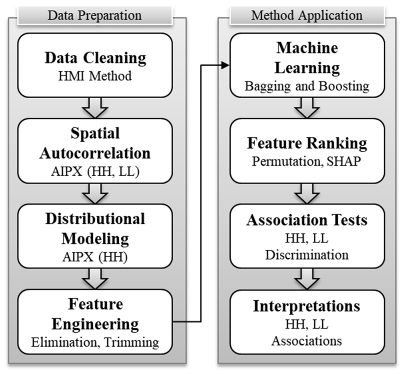
Figure 2.
County clusters of AIPX. The light lines represent the railroad track network.
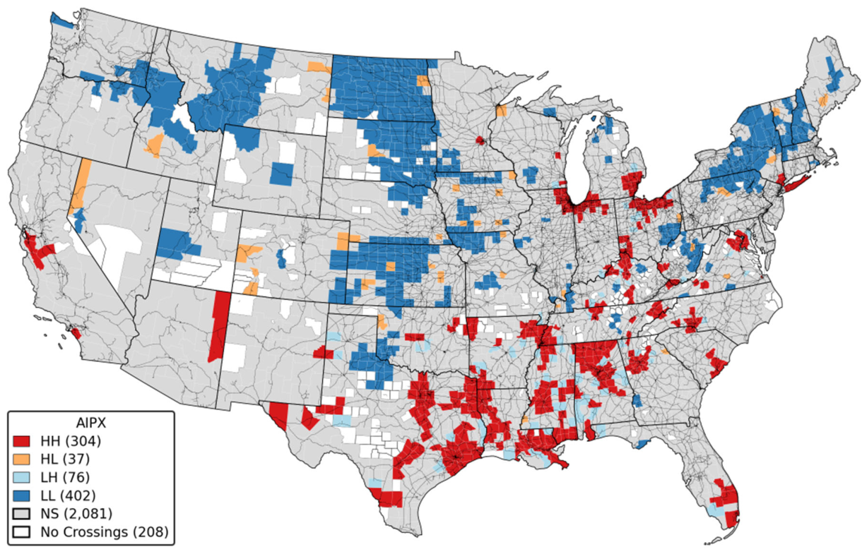
Figure 3.
AIPX HH distribution.
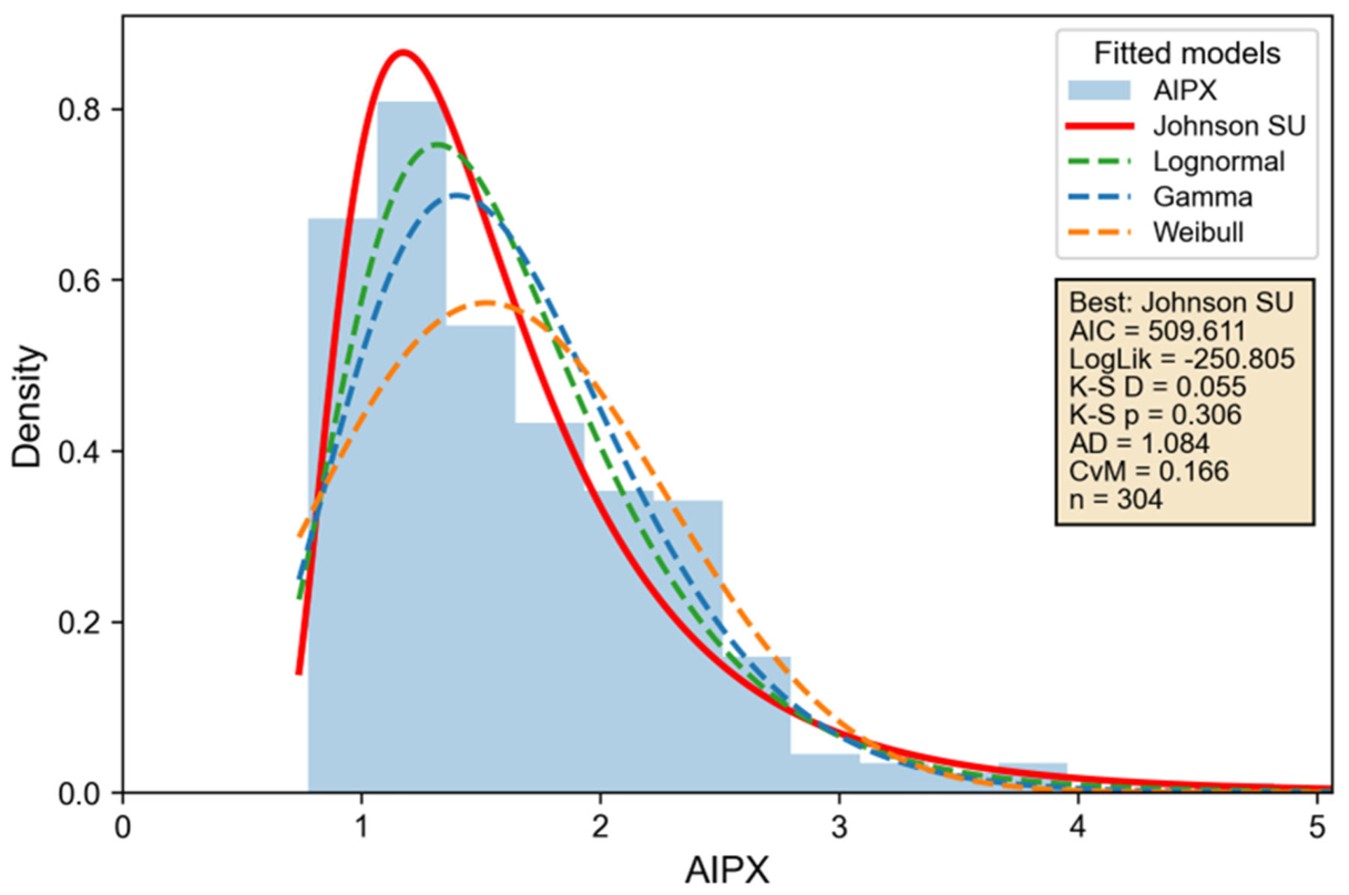
Figure 4.
Recursive feature elimination.
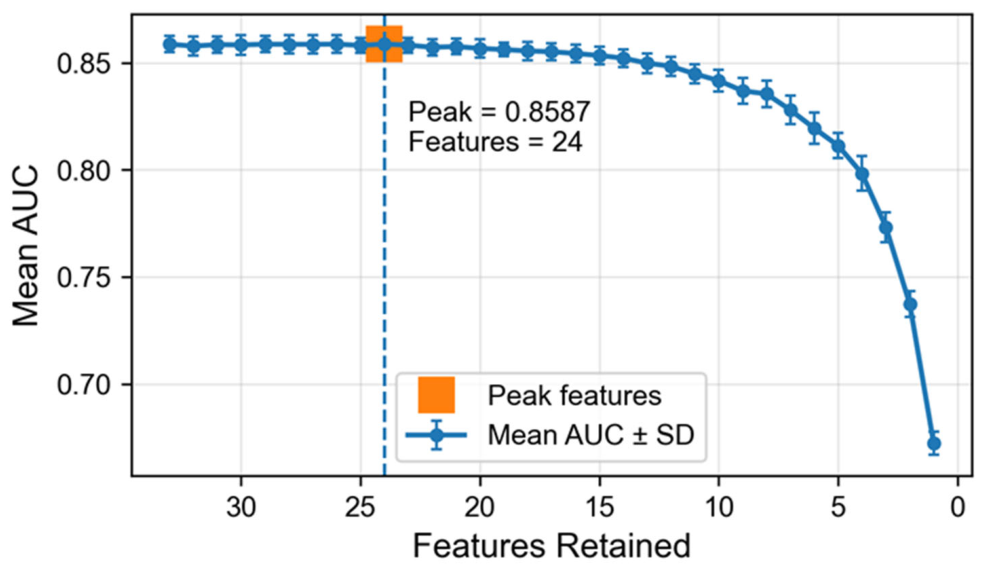
Figure 5.
Distribution of categorical variables and features retained indicated by bars with a solid line border.
Figure 5.
Distribution of categorical variables and features retained indicated by bars with a solid line border.
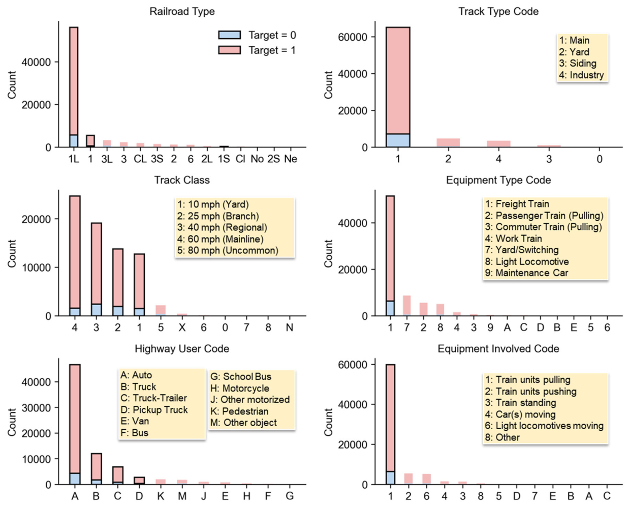
Figure 6.
AUC permutation ranking with the dashed border highlighting the top six features.
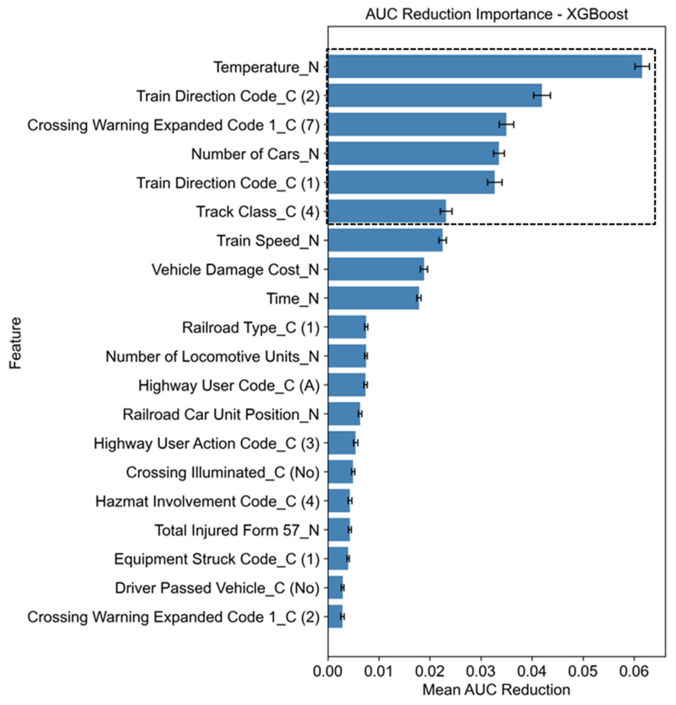
Figure 7.
SHAP ranking with the dashed border highlighting the top six features; up (↑) or down (↓) arrows indicate the direction of that categorical variable association with the HH class.
Figure 7.
SHAP ranking with the dashed border highlighting the top six features; up (↑) or down (↓) arrows indicate the direction of that categorical variable association with the HH class.
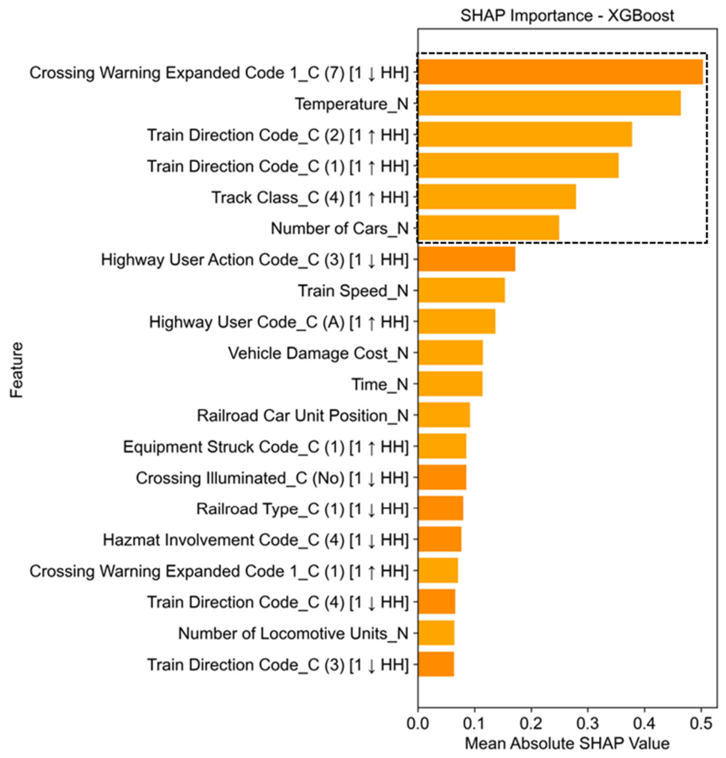
Figure 8.
HH and LL class share of warning types.
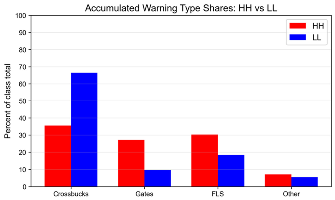
Figure 9.
Train directional shares of the HH and LL classes.
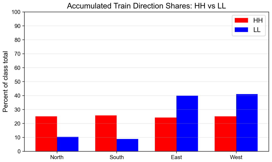
Figure 10.
Temperature distribution and Gaussian overlay of the a) LL class, b) HH class, and c) box plot of each with the vertical line indicating the median, the box representing the interquartile range, the extreme whiskers representing the data extent, and the circles representing outliers.
Figure 10.
Temperature distribution and Gaussian overlay of the a) LL class, b) HH class, and c) box plot of each with the vertical line indicating the median, the box representing the interquartile range, the extreme whiskers representing the data extent, and the circles representing outliers.
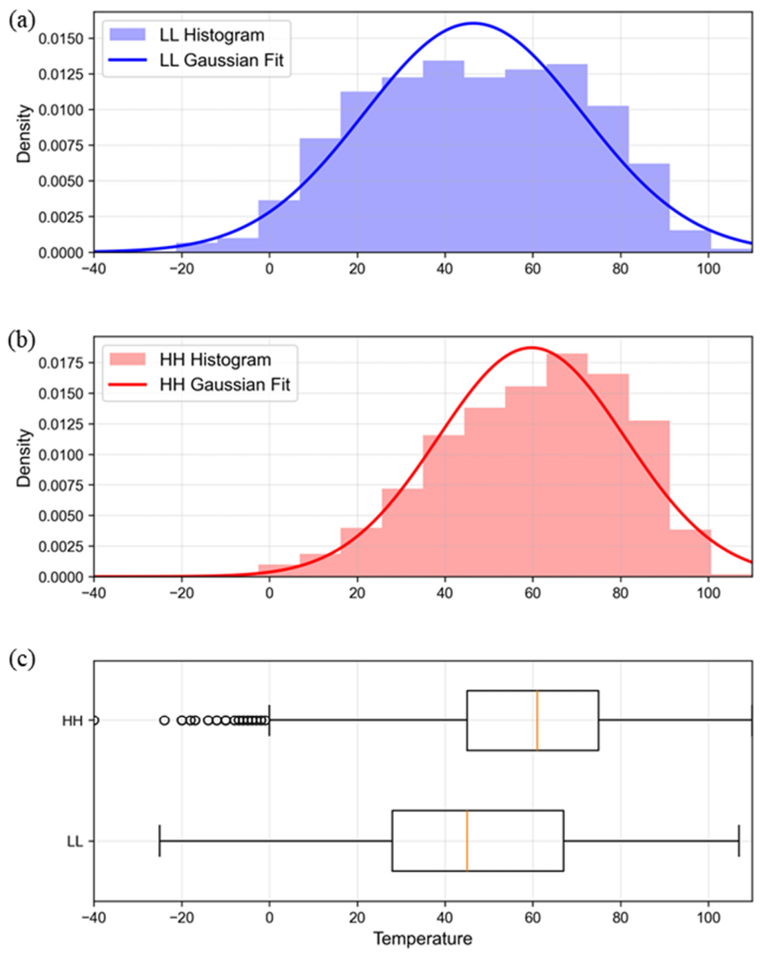

Table 1.
Audit of Data Cleaning Stages.
| Filter | Features | Rows | Description |
|---|---|---|---|
| FRA Incidents | 154 | 250,290 | 51 years of raw incident data (1975 – 2025) |
| Undefined Features | 96 | 250,290 | Drop features with >5% missing values, add “Row ID” key |
| Public/Private Code = “Y” | 96 | 226,170 | Retain public at-grade crossings only |
| Reconciled Counties | 101 | 225,765 | CONUS retained, HMI reconciled, audit features added |
Table 2.
Test Statistics and Distributional Parameters of Models Fitted to AIPX HH Class.
| Model | k | AIC | K–S D | K–S p | AD | CvM | RQQ | r | RPP | α | μ | σ |
|---|---|---|---|---|---|---|---|---|---|---|---|---|
| Johson SU | 4 | 509.61 | 0.05 | 0.31 | 1.08 | 0.17 | 0.13 | 0.99 | 0.02 | -7.22 | 0.54 | 0.02 |
| Lognormal | 2 | 518.50 | 0.06 | 0.17 | 1.49 | 0.24 | 0.06 | 1.00 | 0.03 | 0.37 | 0.00 | 1.51 |
| Gamma | 2 | 534.12 | 0.08 | 0.05 | 2.32 | 0.37 | 0.10 | 0.99 | 0.04 | 7.18 | 0.00 | 0.23 |
| Weibull | 2 | 581.40 | 0.10 | 0.00 | 4.79 | 0.66 | 0.15 | 0.97 | 0.05 | 2.62 | 0.00 | 1.83 |
Table 3.
Audit of Feature Trimming Results.
| Filter Stage | Total | Kept | Dropped % | Dominant Categories |
|---|---|---|---|---|
| HH & LL Clusters | 74,373 | 74,373 | 0 | Homogeneous spatial clusters |
| Railroad Type = [1, 1L, 1S] | 74,373 | 62,062 | 16.55 | Class 1 Railroads |
| Track Type Code = [1] | 62,062 | 54,503 | 10.16 | Mainline tracks |
| Track Class = [1,2,3,4] | 54,503 | 52,051 | 3.3 | Track speed limit classes |
| Equipment Type Code = [1] | 52,051 | 41,171 | 14.63 | Freight trains |
| Equipment Involved Code = [1] | 41,171 | 39,257 | 2.57 | Train units pulling |
| Highway User Code = [A, B, C, D] | 39,257 | 36,488 | 3.72 | Cars and trucks |
| Missing Values | 36,488 | 34,614 | 2.52 | Dropped empty |
Table 4.
Audit of Data Cleaning Stages.
| Filter | Features | Rows | Description |
|---|---|---|---|
| Reconciled Counties | 101 | 225,765 | CONUS retained, HMI reconciled, add fixed state/county to audit |
| Significant Clusters | 39 | 74,373 | Retain HH/LL labeled incidents, drop meta variables |
| Redundant Features | 33 | 74,373 | Drop redundant variables (total vs. breakdown of killed/injured) |
| Unimportant Features | 24 | 74,373 | Recursive AUC feature elimination to maximize mean AUC |
| Category Trimming | 24 | 36,488 | Retain dominant categories (Class, Freight, Mainline, etc.) |
| Undefined Predictors | 24 | 34,614 | Drop incidents with missing predictors before model fitting |
Table 5.
Model Performance Metrics, Runtime Ratio, and Hyperparameter Selection.
| Model | AUC | F1 | RTR | Hyperparameters Grid and Selections in Bold Font |
|---|---|---|---|---|
| XGB | 0.849 | 0.950 | 1.9 | n = [100,200,300]; d = [4,6,8]; η = [0.03, 0.05, 0.1]; s = [0.8, 1.0]; c = [0.8, 1.0] |
| LGB | 0.848 | 0.950 | 17.4 |
n = [100,200,300]; d = [-1, 10, 20]; l = [31,63]; η = [0.03, 0.05, 0.1]; s = [0.8, 1.0]; c = [0.8, 1.0] |
| CB | 0.846 | 0.951 | 7.0 | n = [100,200,300]; d = [4,6,8]; l = [3,5,7]; η = [0.03, 0.05, 0.1] |
| RF | 0.838 | 0.949 | 9.1 | n = [100,200,300]; d = [none, 10, 20]; m = [2,5]; l = [1,2] |
| LR | 0.822 | 0.949 | 1.0 | C = [0.01, 0.1, 1.0, 10.0]; R = [L1, L2] |
| ET | 0.815 | 0.947 | 9.0 | n = [100,200,300]; d = [none, 10, 20]; m = [2,5]; l = [1,2] |
Table 6.
Warning Device Distribution by Spatial Cluster Class (HH vs LL).
| Warning Type | LL Count | LL (%) | HH Count | HH (%) | Δ (HH% − LL%) | Z-statistic | p-value |
|---|---|---|---|---|---|---|---|
| Crossbucks | 2,364 | 66.48 | 11,017 | 35.47 | −31.01 | −35.97 | <0.001 |
| Gates | 343 | 9.65 | 8,440 | 27.17 | 17.53 | 22.75 | <0.001 |
| FLS | 655 | 18.42 | 9,397 | 30.26 | 11.84 | 14.73 | <0.001 |
| Other | 194 | 5.46 | 2,204 | 7.1 | 1.64 | 3.65 | <0.001 |
| Total (N) | 3,556 | 100 | 31,058 | 100 | — | — | — |
Table 7.
Global Test of Independence.
| Statistic | Value |
|---|---|
| Chi-square (χ²) | 1346.25 |
| Degrees of freedom | 3 |
| p-value | <0.001 |
| Cramér’s V | 0.197 |
Table 8.
Directional Distribution by Spatial Cluster Class (HH vs LL).
| Direction | LL Count | LL (%) | HH Count | HH (%) | Δ (HH% − LL%) | Z-statistic | p-value |
|---|---|---|---|---|---|---|---|
| North | 367 | 10.32 | 7,783 | 25.06 | 14.74 | 19.62 | <0.001 |
| South | 315 | 8.86 | 7,986 | 25.71 | 16.85 | 22.3 | <0.001 |
| East | 1,417 | 39.85 | 7,503 | 24.16 | −15.69 | −20.26 | <0.001 |
| West | 1,457 | 40.97 | 7,786 | 25.07 | −15.90 | −20.31 | <0.001 |
| Total (N) | 3,556 | 100 | 31,058 | 100 | — | — | — |
Table 9.
Global Test of Independence.
| Statistic | Value |
|---|---|
| Chi-square (χ²) | 1279.38 |
| dof | 3 |
| p-value | <0.001 |
| Cramér’s V | 0.192 |
Table 10.
Temperature Distribution Descriptive Statistics by Class.
| Class | N | Mean | Median | Std | Min | Q1 | Q3 | Max | IQR | Skew | Kurtosis |
|---|---|---|---|---|---|---|---|---|---|---|---|
| LL | 3,556 | 46.44 | 45 | 24.89 | −25.0 | 28 | 67 | 107 | 39 | −0.07 | −0.75 |
| HH | 31,057 | 59.73 | 61 | 21.33 | −40.0 | 45 | 75 | 110 | 30 | −0.41 | −0.41 |
Table 11.
HH vs LL Temperature Distribution.
| Test | Statistic | Units | p-value | Effect Size | Interpretation |
|---|---|---|---|---|---|
| Welch’s | 30.58 | t | <0.001 | — | Mean difference (HH > LL) |
| M–W | 7.23×10⁷ | U | <0.001 | r_rb = 0.31 | Rank/location difference |
| K–S | 0.23 | D | <0.001 | — | Distributional difference |
| Cohen’s d | 0.61 | d | — | 0.61 | Moderate standardized mean difference |
Table 12.
Gaussian Goodness-of-Fit by HH and LL Classes.
| Class | N | μ | σ | Log-Lik | AIC | KS D | KS p | CvM W2 | CvM p |
|---|---|---|---|---|---|---|---|---|---|
| LL | 3,556 | 46.44 | 24.89 | −16,475.99 | 32,955.99 | 0.067 | <0.001 | 2.74 | <0.001 |
| HH | 31,057 | 59.73 | 21.33 | −139,103.57 | 278,211.15 | 0.082 | <0.001 | 31.87 | <0.001 |
Disclaimer/Publisher’s Note: The statements, opinions and data contained in all publications are solely those of the individual author(s) and contributor(s) and not of MDPI and/or the editor(s). MDPI and/or the editor(s) disclaim responsibility for any injury to people or property resulting from any ideas, methods, instructions or products referred to in the content. |
© 2026 by the authors. Licensee MDPI, Basel, Switzerland. This article is an open access article distributed under the terms and conditions of the Creative Commons Attribution (CC BY) license (http://creativecommons.org/licenses/by/4.0/).
Copyright: This open access article is published under a Creative Commons CC BY 4.0 license, which permit the free download, distribution, and reuse, provided that the author and preprint are cited in any reuse.


