

Submitted:
11 May 2026
Posted:
11 May 2026
You are already at the latest version
Abstract
Aerodynamic drag is one of the two principal external sources of energy loss in on-road vehicles – the other being rolling resistance – and it critically affects the range of battery-electric and fuel cell-electric vehicles. To ensure accurate early-stage analysis such as vehicle range prediction and sizing of energy storage and powertrain components, it is essential to incorporate realistic representations of air resistance. Despite its importance, due to limited data availability air resistance is often simplified using zero crosswind and "nominal air conditions", which tend to underestimate the actual energy required to overcome aerodynamic drag. This approach also fails to capture the variability introduced by changing environmental conditions, leading to significant discrepancies in energy consumption and, consequently, vehicle range. As a result, evaluating system robustness and conducting meaningful trade-off analyses between different vehicles or vehicles configurations becomes challenging. This study demonstrates how publicly available meteorological data can be utilized to quantify long-term variations in aerodynamic drag. By analyzing multiple years of weather observations, we derive realistic distributions of aerodynamic energy losses – capturing not only mean values but also the full range of variability. These distributions enable probabilistic modeling of vehicle performance, thereby supporting robust system design and informed trade-off decisions across various levels of vehicle architecture. To demonstrate this, we compare two different tractor/semitrailer configurations.
Keywords:
vehicle range prediction
; energy consumption
; environmental losses
; air resistance
; weather data
1. Introduction
In vehicles and fast-moving working machines, a significant amount of energy is spent on environmental losses, mainly to overcome air resistance and rolling resistance, see Sandberg (2001), Stenvall (2010), Hariram et al. (2019), Askerdal (2023). For ICEVs, i.e. vehicles powered by internal combustion engines (ICEs), air resistance losses are reported to be up to 45% of the total amount of energy required. This ratio is even larger in battery-electric vehicles (BEVs) due to the vastly higher efficiency of an electric powertrain. All losses negatively affect vehicle range and should therefore be minimized.
When using computer simulation, quantification of the impact on system efficiency must be done using appropriate, representative operating cycles to not fall into the trap of cycle beating i.e. achieving artificial improvements that on paper look impressive but have little to no impact in real operation, see Filla (2012) and Tietge (2015). Using real-life duty cycles in vehicle system analysis and optimization has lately become fashionable but even then, while including elevation and traffic, the effects of weather are usually excluded, for example Ferrara et al. (2021), Hajduk et al. (2025).
Realistic data on the movement and properties of the air are not readily available for most researchers. Wind-Averaged Drag (WAD) analysis, for example in Dalessio et al. (2017), is an attempt at achieving more realistic results using a simplified yaw angle weighting function – although constant wind speed is generally assumed. In Barry (2018) both wind direction and wind speed are used as an improvement, but also this is a simplification.
In Filla (2025, 2026) we utilize quality-assured data from meteorological observations conducted and published by various national/international entities. This results in accurate distributions for wind speed and direction, air density etc. The focus of this publication will be on describing the developed workflow to compute and compare the aerodynamic losses of two trucks, in this case: tractors with semitrailers, aggregated from simulated twice-daily operation over several years on several routes in a specific region. This reproducible workflow can be adapted to other regions and conditions.
2. Air Resistance
Air resistance as a force counter-acting a vehicle’s motion is calculated according to (1), taking as input the air density , airflow velocity , and the vehicle’s corresponding drag coefficient and cross-section .
The ram air experienced by the vehicle moving with speed , i.e. the movement of the vehicle relative to the ground, is to be combined (by means of vector summation) with the wind , i.e. the movement of the air relative to the ground, in order to obtain the total airflow over the vehicle in terms of and yaw angle . Both factors of the product are dependent on .
For competitive reasons vehicle manufacturers are hesitant to disclose values, especially for other airflow angles than . Figure 1 presents two such data sets: “T-ST #1” has been derived by combining, reprocessing and back-calculating from plots and data published in Askerdal (2024) and Volvo Trucks (2013). Set “T-ST #2” is calculated from plots and data published in Dineff et al. (2021). The author of this paper wants to express his sincere gratitude for this data having been made publicly available and hopes that the reprocessed sets visualized in Figure 1 make this data even more accessible to other researchers.
As can be seen in Figure 1, for both tractor/semitrailer configurations have approximately the same air resistance. The curves then diverge and without knowing the specific environmental and operational conditions it is difficult to state with certainty which vehicle will show the lower air drag losses overall and how great the difference will be in real operation – even if the vehicles are used in the exact same circumstances. Knowing the continuously changing airflow matters because the yaw angle determines the value, which in turn affects the momentary power loss due to air drag.
3. Analysis of Time-Series Data
In Filla (2026) we describe how synthetic time-series data have been created: an ensemble of 11 routes is run bi-directional, twice a day over a period of 5 years; and the simulated vehicle data are augmented with observed meteorological data as listed in Table 1, acquired from the Swedish Meteorological and Hydrological Institute (SMHI) and the Swedish Road Authority (Trafikverket). The latter has graciously provided us with data from their long-term archive of the Road Weather Information System, Vägväderinformationssystem (VViS).
In Abel et al. (2022) the authors argue for the use of highly resolved wind forecasts. The same argument can be made for observations, and likely the same methodology could be used to calculate wind data in high resolution from observational data. However, such upscaled data is not available at this time, therefore the low-resolution observations must suffice.
In Figure 2 all measurement stations from Trafikverket are plotted, with the dot color expressing how many neighboring stations there are within a 30 km radius. Not surprisingly, the density is the highest in the major urban areas Stockholm, Göteborg and Malmö.
Algorithms for efficiently augmenting time-stamped vehicle positions with station-based (and grid-based) meteorological data have been described in Filla (2025).
Figure 3 shows that the routes simulated in this study cover essentially all major roads in southern Sweden. The ensemble is therefore considered to be representative for long-haulage truck operations in this whole region, rather than representing just a single route or area.
Each generated route fully describes the vehicle movement with the following parameters: timestamp, longitude, latitude, incremental distance, cumulative distance, elevation, heading, speed, and speed limit. The routes have been generated using a combination of calls to the APIs from Google Maps and HERE to achieve results or obtain additional data that are not offered by either one service provider alone.
First, all routes between respective start and destination have been generated specifically for a truck using HERE. The paths returned feature as many sections and points as HERE deems necessary to fully describe each trip. The route points offered are not spread out in regular intervals but placed wherever a decision needs to be made by the driver or supporting information is available for guidance. Using the Elevation API of Google Maps the paths have been resampled to consist of (mostly) equidistant points. In our study we chose 25 meters as sampling distance. The points returned (now also including elevation data) have then been matched back to the road network in HERE; and the spans returned by HERE in the first step have been fitted to the new set of (mostly) equidistant points. These spans contain the speed limits as well as typical traffic speed – which made it possible to create a time vector, moving the virtual truck along the path at the desired pace, following the traffic rhythm typical for this part of the route, obeying the legal speed limits and possibly even being limited to a preset lower speed. Finally, the truck’s heading along the path has been calculated from the sequence of coordinates of the resampled, tightly placed points.
We have also investigated possible improvements to reduce the significant amount of time required to collect and process all data. For example, we examined the difference a sampling distance of 1000 m instead of 25 m would make. Figure 4 shows that when calculating with the vehicle T-ST #1 the coarser sampling leads to result deviations in the range from –10% to +15% compared to the original setup.
At first glance such large deviations might be surprising. An explanation can be found in the way these new routes have been created: instead of simply extracting every 40th sample from the routes with 25 m equidistant sampling we created a new set of the same routes following the previously described process, but with 1000 m sampling distance. This was done several months later, and it turned out that the speed limit of many road sections had changed by then. Also, for some parts the typical speed of traffic was different, likely due to setting up or removing road construction sites. See Figure 5 for two examples.
This of course affects the simulated air drag losses. However, these deviations should not have much impact in a comparison of vehicles with different aerodynamic profiles as all would be affected alike. We nevertheless used the original routes (25 m).
Figure 6 shows the results in terms of air drag losses for the two vehicles configurations T-ST #1 and #2 in comparison. While the upper two histograms, showing the distribution of the specific energy losses for air resistance look similar in both cases, the lower two plots reveal that the truck/semitrailer configuration #2 shows up to 15% higher energy losses in a trip-by-trip comparison with configuration #1 (calculated over all 2×80344 simulated vehicle journeys), with a mean value of 3.7% – large enough to matter in commercial operation.
Going back to Figure 1 we can now confidently conclude that configuration T-ST #2 is clearly inferior, despite featuring the same air resistance at airflow angle as T-ST #1. The higher values up to are not compensated for by lower air resistance above this yaw angle – also because high yaw angles are increasingly uncommon in real operation.
The plot in the upper right in Figure 7 shows that yaw angles above 12.5° account for less than 5% of all time. This plot also shows that yaw angles below 2.5° account for less than 50% of all time. It would thus be a significant mistake to not consider airflow angles .
Furthermore, the upper left plot in Figure 7 depicts that airflow speed is dominated by the vehicle speed – which is logical given that the created routes feature a high amount of highway driving and that extreme wind is unusual in southern Sweden.
However, dominant wind patterns do exist, for example at or near the west coast of Sweden wind is more likely to come from south-west. Therefore, long-term over the course of the simulated five years of truck operation, driving from Örebro to Göteborg should show higher energy losses than the other way around.
Figure 8 shows that there are indeed small differences between the airflow distributions of both travel directions; and Figure 9 proves that these differences are significant enough to result in higher air drag losses for the vehicle driving south-west.
Travelling with T-ST #1 south-west from Örebro to Göteborg (route #12) shows on average in a trip-by-trip comparison 13.2% higher air drag losses compared to the same vehicle driving at the same time the other way around (route #1), with the difference ranging from –50% to +150% during the five-year period analyzed in our study (Figure 9).
Such comparisons on a trip-by-trip basis, calculated sample-by-sample, are only possible with a lot of time-series data at sufficient resolution. The downside is a large amount of data that needs to be handled, which presents challenges for memory and storage use as well as processing time.
4. Analysis Using Weighted Distributions
The alternative to analyzing time-series data is the use of aggregated data in the form of weighted distributions, similar to the aforementioned WAD method. Figure 7 shows the time-weighted distribution of airflow angle and speed. The two-dimensional probability density function (PDF) visualized in the lower plot in Figure 7 can be used to calculate air drag and associated power losses with reasonable precision. It is also feasible to calculate the mean specific energy loss and the ratio between vehicles with different aerodynamic profiles.
Calculation can be either performed directly using the bin edges of the PDF in Figure 7 to compute the corresponding interval ranges of air drag and power loss – or by generating a sufficiently large ensemble of randomly generated airflow data with a distribution matching the PDF, essentially a Monte Carlo simulation. Both approaches yield comparable results.
Calculating these results presented the problem of how to account for linked probability distributions: we only have the PDF for airflow (Figure 7) but would also need to know how other air properties vary, as well as the vehicle speed. None of these are independent from airflow.
Fortunately, an analysis of the variation in air density, itself a result of variations in air temperature, humidity and pressure (including changes in elevation), showed that in our study the resulting air density is normal distributed with a median value very close to the international standard value of 1.225 kg/m³ (Figure 10). It is therefore acceptable to simply calculate with this constant standard value, which the upper plot in Figure 11 proves.
Figure 11 shows that the dynamic air pressure, drag force and associated power loss results from the Monte Carlo simulation match the data from the time-series calculations fairly well.
The upper left plot in Figure 7 also provides the PDF of vehicle speed but we cannot determine which vehicle speed sample is linked to which airflow sample. We have previously concluded that vehicle speed dominates the airflow speed distribution. As an approximation we can therefore use the airflow speed to calculate power loss from air drag force. The lower right plot in Figure 11 proves that this is an acceptable simplification.
Going further from power loss to calculate the distribution of specific energy losses for different aerodynamic profiles is out of reach because the PDF in Figure 7 does not disclose which individual airflow samples, in extension leading to the power loss distribution, are to be combined to one journey. We can, however, calculate the mean specific energy losses for vehicles with different aerodynamic profiles by simply aggregating all air drag force samples. Starting with the equation for drag force (1) we calculate the associated energy loss as
With specific energy loss being energy loss per trip distance D and the rough approximation that we get
Roughly approximating further that we get
Again, by taking just the airflow distribution as input we have lost the individual samples. All we can calculate is the total amount of time per interval of power loss. Energy loss as the product of power loss and duration is out of reach since we do not have all the single power and duration samples, we only know the total sum. This is not enough to recreate the energy distribution, but it is enough to calculate the mean value of the specific energy loss.
Figure 12 shows that the ratio of mean specific energy loss for T-ST #2 vs. #1 calculated with the approximations above is reasonably near the true mean value from the time-series calculations. The histogram underneath is taken from Figure 6 (lower right plot) and shows that the distribution is asymmetric with the mean value located to the lower end of the distribution range.
In summary, using only the two-dimensional PDF of airflow we can approximate rapidly and reasonably well the average impact of different aerodynamic profiles on specific energy loss in the vehicle.
5. Discussion
The assumption underlying the presented work is that the meteorological data utilized are representative and of high quality. Both aspects, as well as the limitations of the acquisition method, have been elaborated on in our previous publications Filla (2025, 2026). The representativeness is a double-edged sword as this means that the geographic region of application is encoded into the dataset, which in our case is southern Sweden. A study of a different geographic region requires acquisition of a different data set. Furthermore, these routes also encode a specific vehicle application, long haulage with a higher amount of continuous high-speed operation than what is the case in regional or city distribution.
Finally, it must be pointed out that while in the past the use of long-term historic observations of meteorological conditions might have been representative for future weather, in our times of climate change this cannot be guaranteed. It is advised to continuously verify and acquire new meteorological data from recent observations.
6. Conclusions
Two different approaches have been presented. Both can be used to calculate the effect of different aerodynamic profiles but are suitable for different applications. The comprehensive time-series approach is resource-demanding but yields high-quality results if the meteorological data utilized are of sufficient quality. It is highly suitable for detailed analysis.
The approach utilizing the airflow distribution calculated with the time series can either entail a Monte Carlo simulation that follows the original airflow distribution or simply a calculation with the bin edges and associated probabilities. Either way the computation is very fast and yields approximate results that can be used for initial screening of concepts.
Acknowledgments
Financial support from FFI, Vehicle Strategic Research and Innovation, for project P2022-00952 “CONDORE – Customer Oriented Operations Research for Electrification” within the FFI Nollutsläpp program, administered by the Swedish Energy Agency, is hereby gratefully acknowledged.
References
- Abel, R.; Pegel, L.; Waldmann, A. On the Importance of Highly Resolved Wind Forecasts for Range Estimation. In Proceedings of the 22. Internationales Stuttgarter Symposium; Bargende, M., et al., Eds.; 2022; pp. 187–196. [Google Scholar] [CrossRef]
- Askerdal, M. On motion Resistance Estimation and Modeling for Heterogeneous Road Vehicles. Licentiate Thesis, Chalmers University of Technology, Göteborg, Sweden, 2023. Available online: https://research.chalmers.se/publication/535577.
- Askerdal, M.; Fredriksson, J.; Laine, L. Development of simplified air drag models including crosswinds for commercial heavy vehicle combinations. Veh. Syst. Dyn. 2024, 62(5), 1085–1102. [Google Scholar] [CrossRef]
- Barry, N. A New Method for Analysing the Effect of Environmental Wind on Real World Aerodynamic Performance in Cycling. In ISEA; Espinosa, H., Rowlands, D., Shepherd, J., Thiel, D., Eds.; MDPI: Basel, 2018; Volume 2018 2, (69, pp. 211–218. [Google Scholar] [CrossRef]
- Dalessio, L.; Bradley, D.; et al. Accurate Fuel Economy Prediction via a Realistic Wind Averaged Drag Coefficient. SAE Int. J. Passeng. Cars-Mech. Syst. 2017, 10(1), 265–277. [Google Scholar] [CrossRef]
- Dineff, A.; Upadhyaya, A.; et al. Aerodynamic investigations of a simplified truck under high yaw wind conditions. Master Thesis, Chalmers University of Technology, 2021. Available online: https://odr.chalmers.se/items/7de498c8-9c62-40dd-8980-31b0c102b8e2.
- Ferrara, A.; Jakubek, S.; Hametner, C. Energy management of heavyduty fuel cell vehicles in real-world driving scenarios: Robust design of strategies to maximize the hydrogen economy and system lifetime. Energy Convers. Manag. 2021, vol. 232, 113795. [Google Scholar] [CrossRef]
- Filla, R. Representative Testing of Emissions and Fuel Consumption of Working Machines in Reality and Simulation. SAE Tech. Pap. 2012, 2012-01-1946. [Google Scholar] [CrossRef]
- Filla, R. Using Weather Data for Improved Analysis of Vehicle Energy Efficiency. Data 2025, 10(3), 31. [Google Scholar] [CrossRef]
- Filla, R. Study of Long-Term Variation of Air Resistance of a Tractor with Semitrailer Using Recorded Weather Data Together with Vehicle Data. SAE Int. J. Commer. Veh. 2026, 19(2), 1–16. [Google Scholar] [CrossRef]
- Hajduk, P.; Ranta, M.; Farzam Far, M.; et al. Enhanced socially oriented mission-based driving cycles generation and simulation framework for light electric vehicles. Humanit. Soc. Sci. Commun. 2025, 12(1), 1166. [Google Scholar] [CrossRef]
- Hariram, A.; Koch, T.; Mårdberg, B.; Kyncl, J. A Study in Options to Improve Aerodynamic Profile of Heavy-Duty Vehicles in Europe. Sustainability 2019, 11(19), 5519. [Google Scholar] [CrossRef]
- Sandberg, T. Heavy Truck Modeling for Fuel Consumption: Simulations and Measurements. Licentiate Thesis, Linköpings Universitet, Linköping, Sweden, 2001. Available online: https://urn.kb.se/resolve?urn=urn:nbn:se:liu:diva-145953.
- Stenvall, H. Driving resistance analysis of long haulage trucks at Volvo. Master Thesis, Chalmers University of Technology, Göteborg, Sweden, 2010. Available online: https://publications.lib.chalmers.se/records/fulltext/133658.pdf.
- Tietge, U.; Zacharof, N.; et al. From Laboratory to road: A 2015 update of official and "real-world" fuel consumption and CO2 values for passenger cars in Europe. In International Council On Clean Transportation Europe (2015); 2015; Available online: https://publications.tno.nl/publication/34622260/35ZR9j/tietge-2015-laboratory.pdf.
- Volvo Trucks. PERF Users Manual. Drag Coefficient (CD), Typical values FH/FM. 2013. Available online: https://vbi.truck.volvo.com/portal/perfman/020_terminology/drag_coefficient_%28cd%29.htm.
Figure 1.
Drag area for two tractor/semitrailers.
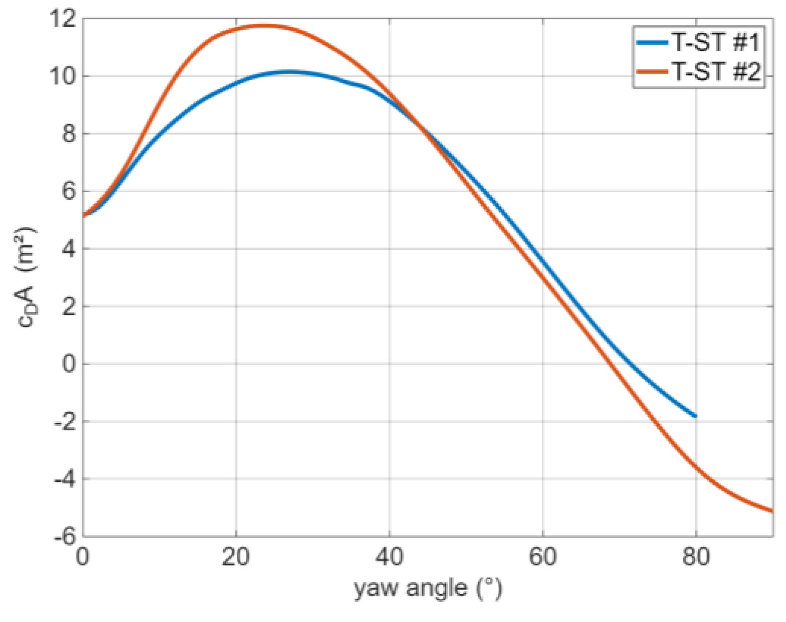
Figure 2.
Station density (Trafikverket).
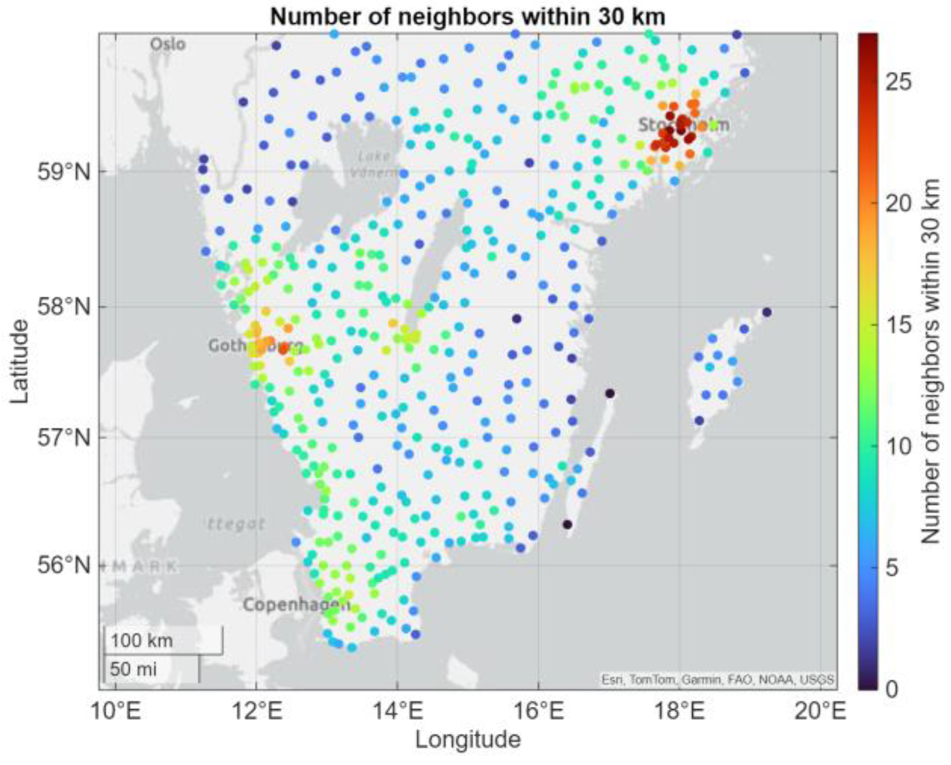
Figure 3.
Simulated routes in southern Sweden.
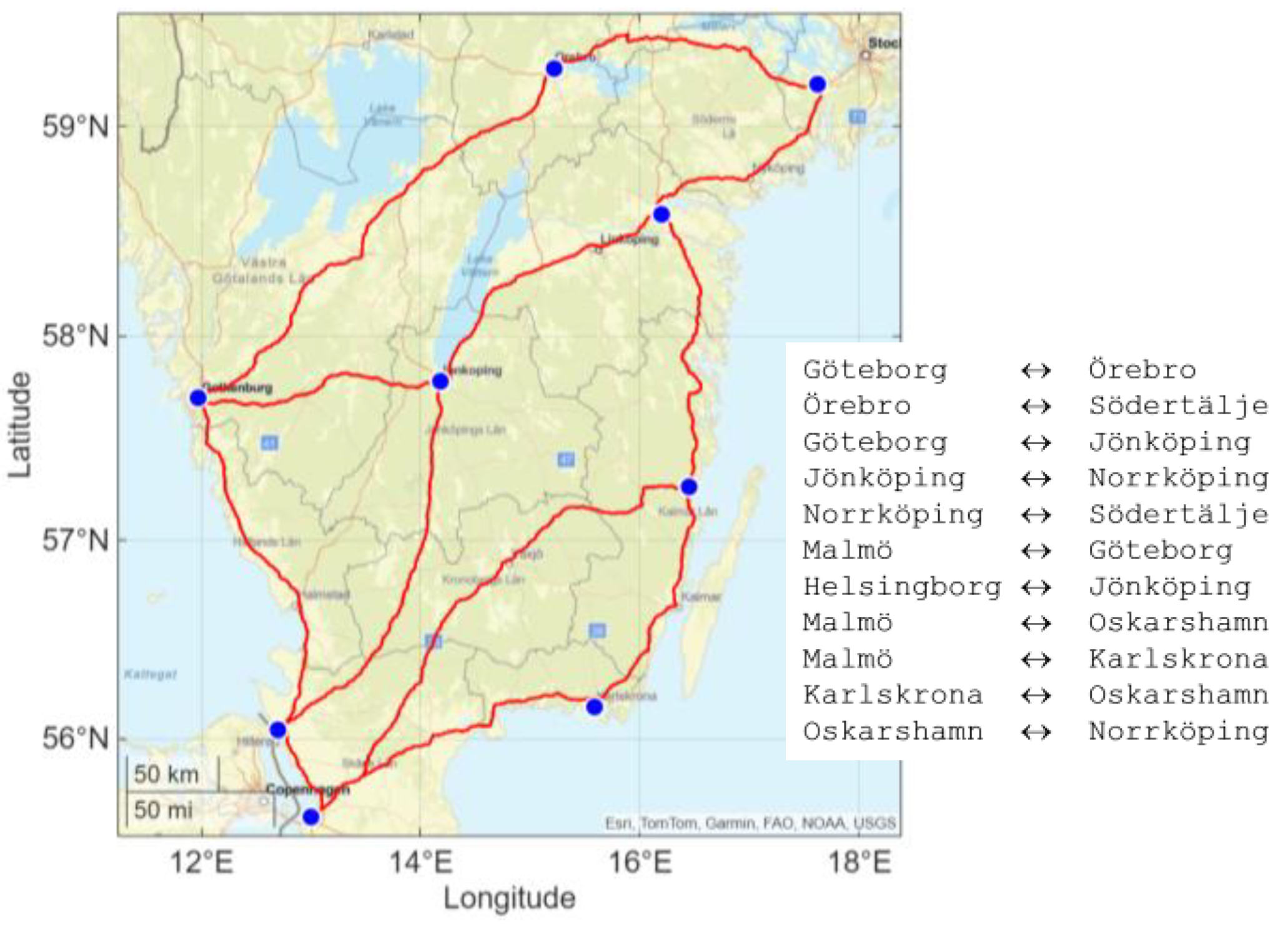
Figure 4.
Effect of increased step size for equidistant sampling.
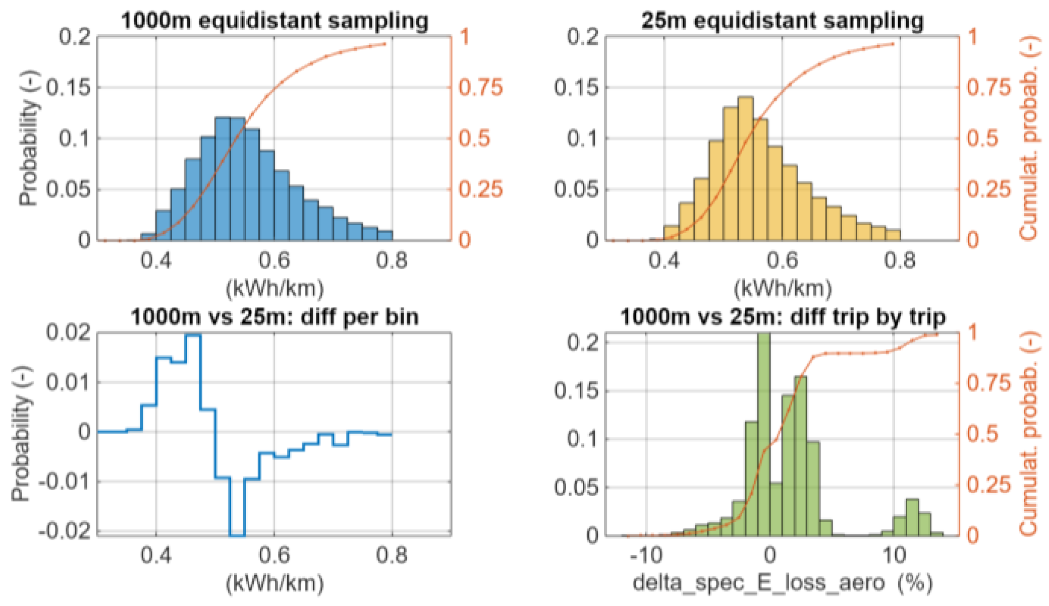
Figure 5.
Different vehicle speeds for 1000 m vs. 25 m sampling.
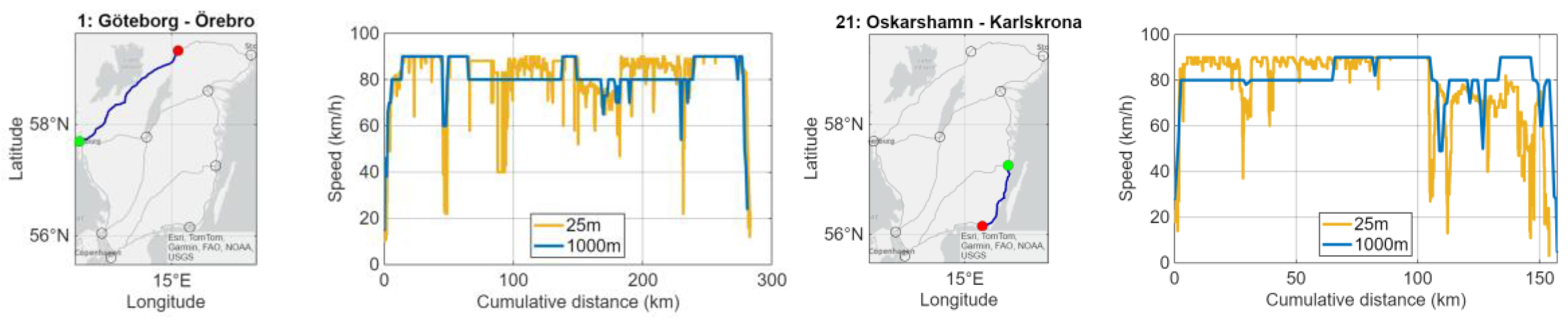
Figure 6.
Comparison of air drag losses T-ST #2 vs. #1.
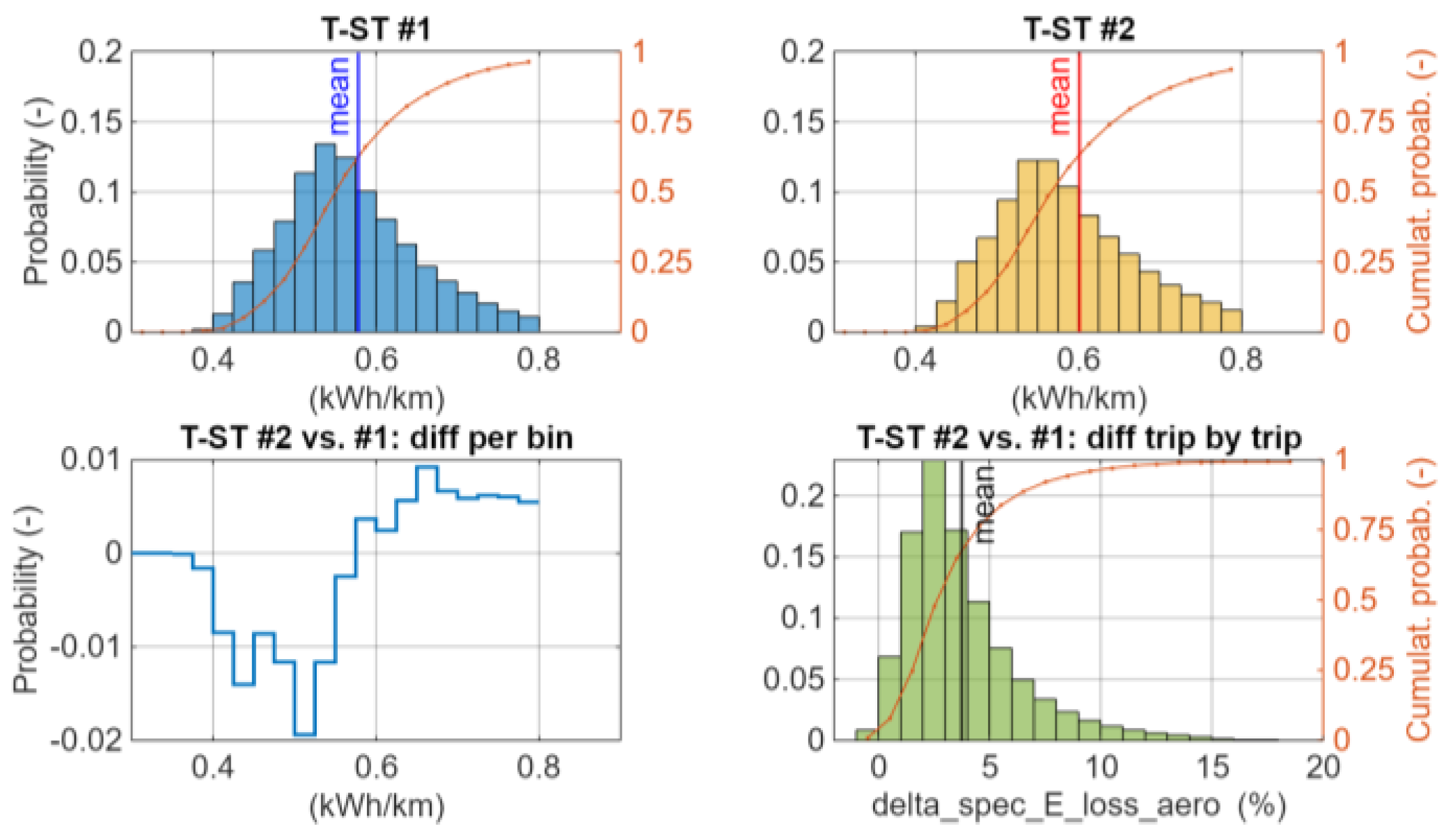
Figure 7.
Airflow distribution over all trips, time-weighted.
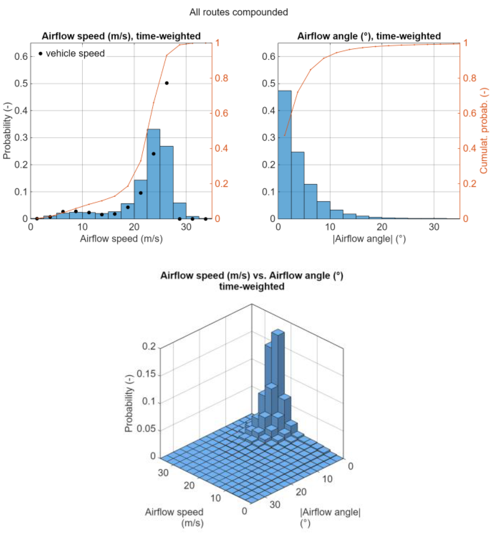
Figure 8.
Airflow distribution for routes #1 and #12.
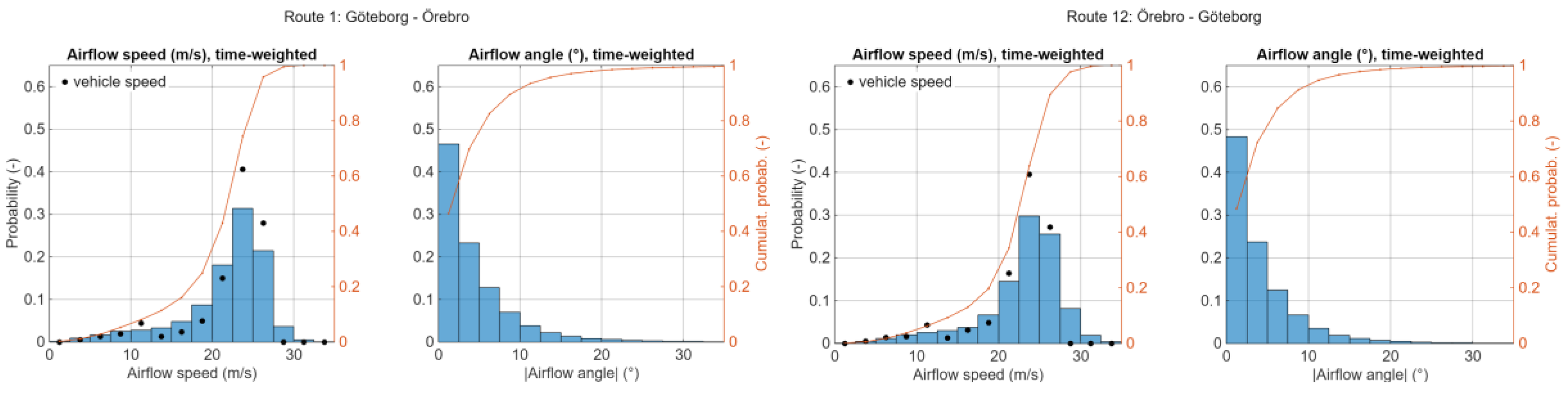
Figure 9.
Comparison of air drag losses for routes #1 and #12.
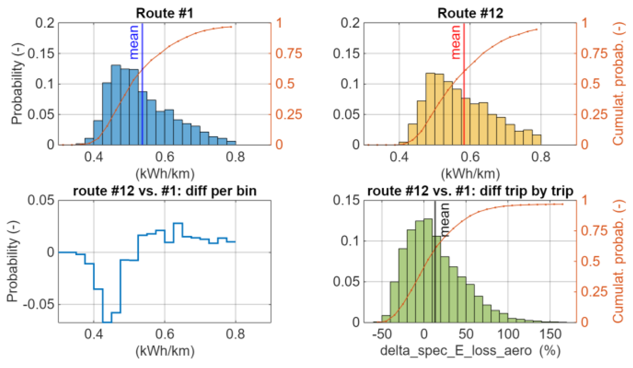
Figure 10.
Air density distribution resulting from time-series calculations (STD = standard value of 1.225 kg/m³).
Figure 10.
Air density distribution resulting from time-series calculations (STD = standard value of 1.225 kg/m³).
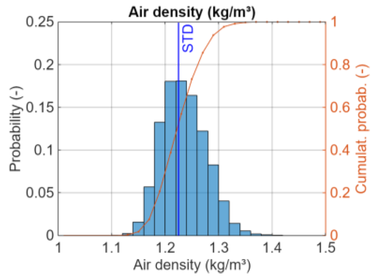
Figure 11.
Comparison of results from Monte Carlo simulation with time-series calculation (calculated for T-ST #1).
Figure 11.
Comparison of results from Monte Carlo simulation with time-series calculation (calculated for T-ST #1).
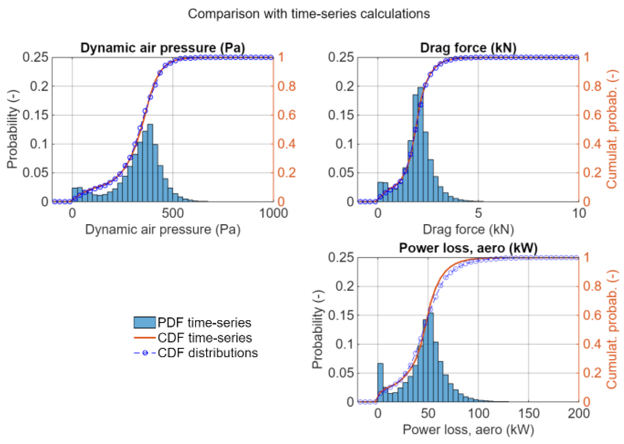
Figure 12.
Mean specific energy loss of T-ST #2 vs. #1: result from calculation with distribution vs. time-series.
Figure 12.
Mean specific energy loss of T-ST #2 vs. #1: result from calculation with distribution vs. time-series.
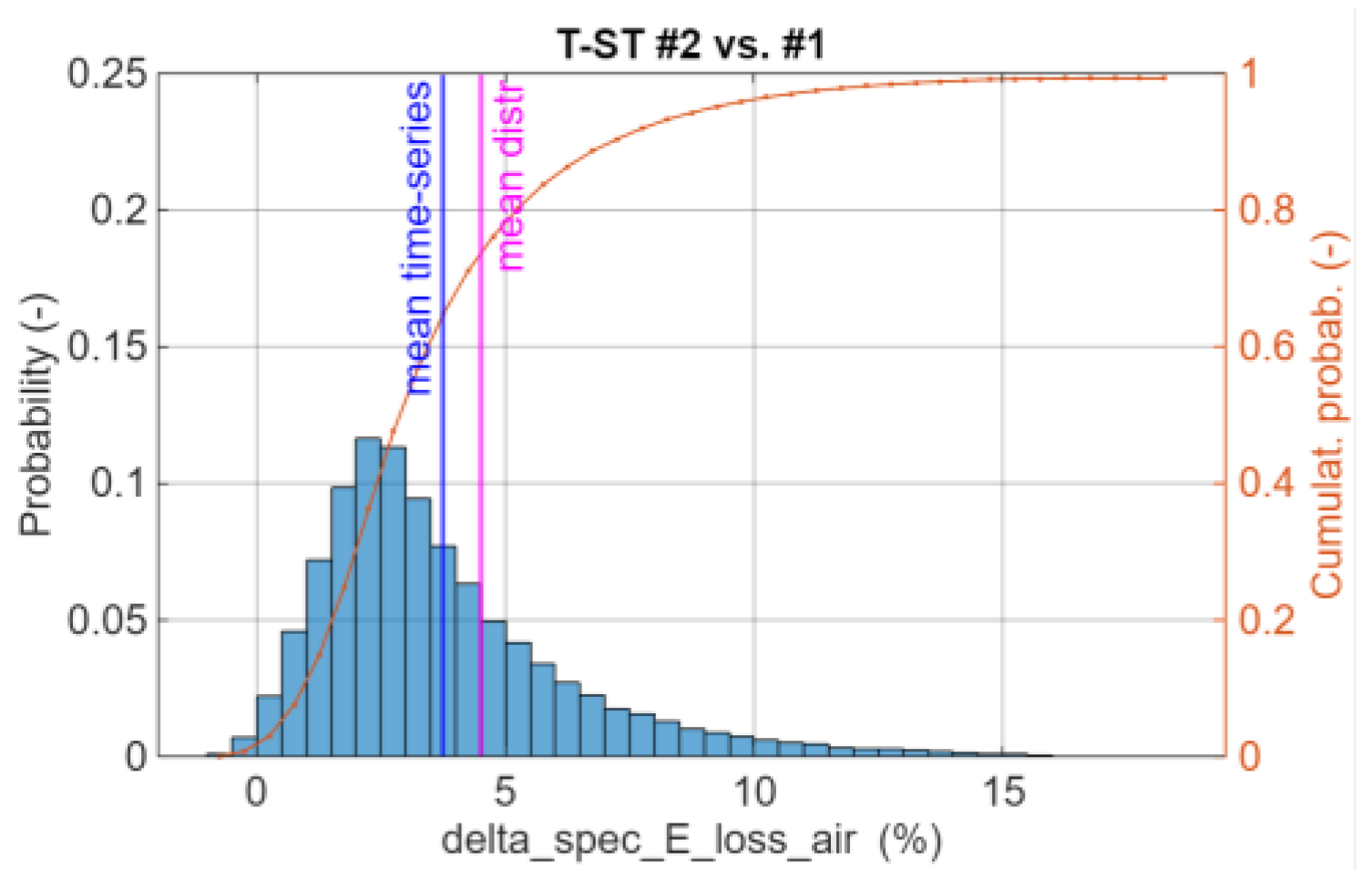

Table 1.
Extracted meteorological data.
| Provider | Parameter |
|---|---|
| Trafikverket | air temperature, wind speed, wind direction |
| SMHI | air pressure, air humidity |
Disclaimer/Publisher’s Note: The statements, opinions and data contained in all publications are solely those of the individual author(s) and contributor(s) and not of MDPI and/or the editor(s). MDPI and/or the editor(s) disclaim responsibility for any injury to people or property resulting from any ideas, methods, instructions or products referred to in the content. |
© 2026 by the authors. Licensee MDPI, Basel, Switzerland. This article is an open access article distributed under the terms and conditions of the Creative Commons Attribution (CC BY) license (http://creativecommons.org/licenses/by/4.0/).
Copyright: This open access article is published under a Creative Commons CC BY 4.0 license, which permit the free download, distribution, and reuse, provided that the author and preprint are cited in any reuse.


