A Simulation Study to Analyze the Inference of Weather Parameters from Changes in Snowcover

1. Introduction

Snow is a porous material composed of ice, water and air, due to low melting point of ice (0 degree C) its properties change rapidly with small changes in its surrounding environment (Brun et al. 1992). This leads to complex changes in snowcover properties over time due to weather and radiation, conversely the snowpack also affects the local meteorological processes near it (Cohen, J., and D. Rind, 1991). Knowledge of this complex interaction is required in several applications e.g: avalanche forecasting (Lehning et al. 2002; Morin et al. 2020), weather research (Barnet et al. 1988; Thackarey et al. 2019; Vayrus 2007), hydrology estimates (Lehning et al. 2006; Woods 2009), assessment of snow stability (Viallonn et al. 2022) etc. Therefore considerable effort has been done in development of complex models to describe the dependence of snowcover on weather and radiation processes.

SNOWPACK (Lehning et al. 2002) is a model that can accurately simulate several important properties of snowcover given weather and radiation parameters affecting it. The SNOWPACK model takes as input a time-series of some weather and radiation parameters at a site (usually collected using an automatic weather station) and outputs the resulting time series of snowcover states at the site. SNOWPACK models several processes affecting snowcover metamorphism by using data from past experiments conducted on snow under controlled laboratory conditions. (Lehning et al. 2002) provide the processes modelled and their mathematical representations implemented in SNOWPACK model. The model has been validated in a large number of field studies conducted by several researchers, the results of model output are usually in strong agreement with the field measurements.

Since a deterministic model mapping weather and radiation parameters to snowcover states is known, we may expect an inverse relation mapping the time series of snowcover states at a site to the weather and radiation time series that caused those states. This study tries to find such an inverse relation, to the best of our knowledge such an attempt has not been published before. We mapped a time series of snowcover surface states to its corresponding time series of weather and radiation (meteorological) vectors. The series of meteorological data vectors was collected using an automatic weather station, the series of snowcover surface states was obtained from data simulated using SNOWPACK model. We have used simulated data for snowcover surface (instead of actual data) due to difficulty and expense of collecting actual snow surface data in field, the simulated data was generated by the rigorously validated SNOWPACK model. Our work can be interpreted as a preliminary study to analyze the feasibility of finding the inverse mapping, such a study using simulation data can help reduce the risk of failed experiments in field and can be done at a very low cost.

Our results (using simulated snowcover data) were positive and show that snowcover time-series contains important information about meteorological variables and can be used to make precise inferences about meteorological processes near it. In this work we have identified some conditions required to make precise inferences using machine learning models and explored certain applications of these results. In particular applications of these results to reduce the cost of instrumentation for meteorological measurements at a large scale have been analyzed in detail. We have compiled information about the cost of different sensors required for snow surface measurements and compared the cost of our inference technique with usual measurement techniques. We found that a combination of sensors for snow surface measurements coupled with modelling techniques can be used to find meteorological parameters at a lower cost. We also propose the applications of these results as input to downscaling algorithms for numerical weather prediction and meteorological parameter interpolation algorithms.

1.1. Related Work

Work on effect of snowcover on local climate maybe considered as work related to this study, several studies regarding this have been conducted (Barnett 1988; Cohen and Rind 1991; Thackeray et al. 2022; Vayrus 2007; Woods 2009). All such studies relate the bulk properties of snowcover to the local climate, however our work focuses on much smaller scale and relates the microstructural properties of snow to its immediate surrounding environment.

(Boyarskii and Tikhonov; 2000) relate the snowcover stratigraphy to its emitted microwave radiation. Attempts have been made to find certain snowcover properties from emitted radiation (Xiao et al. 2021; Schaffhauser et al. 2008).

2. Materials and Methods

2.1. Mathematical Formulation of Inverse Problem and Modelling Approach

We define the mathematical notation for surface snow and surface meteorological parameters, these parameters vary with respect to time and space. The following definitions will be used to express this variation conveniently:

Definition 1.

We represent the state of near surface snow at a point $P$on time $t$by a vector of real numbers denoted by $S_t\left(P\right)$. The exact construction of this vector from physical/simulated snowpack properties is given in Appendix B.

Definition 2.

The weather and radiation parameters affecting the snowpack at point $P$on time $t$is represented by a vector of real numbers $W_t\left(P\right)$. The exact construction of this vector is detailed in Section 2.3.

Note: We only consider the state of near surface snow (instead of deeper snow) in $S_t\left(P\right)$, this is because of following reasons:

1. It is simpler to measure near snow surface parameters instead of below surface parameters.

2. Surface snow is more responsive to weather changes than below surface snow, therefore state changes of surface snow are more relevant than state changes of below surface snow in the inference of weather.

If the parameters $W_t\left(P\right)$ are known, $S_t\left(P\right)$ can be determined using well known numerical model SNOWPACK. To formulate the reverse problem, we consider a time series of snowpack and meteorological parameters sampled at regular time intervals denoted by sequences: $S_1\left(P\right)$,$S_2\left(P\right),\dots .,S_T\left(P\right)$ and $W_1\left(P\right)$,$W_2\left(P\right),\dots .,W_T\left(P\right)$ respectively. We assume that at time-step $t$, $S_{t+1}\left(P\right)$ is a function of $S_t\left(P\right)$ and $W_t\left(P\right)$. Informally this means that next state of snowpack ($S_{t+1}\left(P\right)$) is determined by its present state ($S_t\left(P\right)$) and the present meteorological state ($W_t\left(P\right)$) (a reasonable assumption also made in snow simulation models). We represent this dependence as equation,

$$S_{t+1}\left(P\right)=\mathit{f}(S_t\left(P\right),W_t\left(P\right)),$$

where $\mathit{f}$ denotes the real valued function mapping $S_t\left(P\right),W_t\left(P\right)$ to $S_{t+1}\left(P\right)$.

We focus on finding an inverse mapping for the meteorological parameters, we wish to find a function $\mathit{g}$ such that

$$W_t\left(P\right)=\mathit{g}(S_{t+1}\left(P\right),S_t\left(P\right)).$$

Since the mapping $\mathit{f}$ is defined by a very complex simulation model, inverting it explicitly to find $\mathit{g}$ is not feasible. Therefore a machine learning based approach has been used to determine a map ${\mathit{g}}_{\mathit{\theta }}$ ($\theta$ denotes the model parameters) analogous to $\mathit{g}$, we use this map to determine $W_t\left(P\right)$ from $S_{t+1}\left(P\right),S_t\left(P\right)$ and a set of meteorological parameters $W_t\left(Q\right)$ collected at a point $Q$near $P$ i.e:

$$W_t\left(P\right)={\mathit{g}}_{\mathit{\theta }}(S_{t+1}\left(P\right),S_t\left(P\right),W_t\left(Q\right))$$

We have additionally included the parameters $W_t\left(Q\right)$ to improve the performance of our model: the intention of including $W_t\left(Q\right)$ is to add meteorological data recorded at nearby locations to the inversion process. $W_t\left(Q\right)$ can be thought of as an estimate of the required output $W_t\left(P\right)$, the mapping ${\mathit{g}}_{\mathit{\theta }}$ improves this estimate using the snow surface parameters $S_{t+1}\left(P\right),S_t\left(P\right)$. In this formulation the performance of the inversion map depends on the accuracy of the estimates $W_t\left(Q\right)$ (i.e their closeness to $W_t\left(P\right)$) and the relevant information about $W_t\left(P\right)$ contained in the snow-surface data $S_{t+1}\left(P\right),S_t\left(P\right)$. When $W_t\left(Q\right)$ is very close to $W_t\left(P\right)$, it contains all information required for the prediction of $W_t\left(P\right)$, if $W_t\left(Q\right)$ is very far then it gives no useful information and prediction is based solely on snow-surface information in $S_{t+1}\left(P\right),S_t\left(P\right)$.

When interpreted as information sources, the estimates $W_t\left(Q\right)$ can be obtained from numerical weather prediction models or instrumentation at nearby locations, there availability is usually not a serious problem in model application. Experimentally we find that inclusion of $W_t\left(Q\right)$ improves the results significantly over just using $S_{t+1}\left(P\right),S_t\left(P\right)$ for inversion, furthermore we found experimentally that the estimates don’t have to be very accurate to give reasonable performance. A detailed discussion about the effect of parameters $W_t\left(Q\right)$ has been provided in the results section of this paper, in our approach this inclusion plays an important role as information in the snow-surface alone was insufficient or unusable to get reasonable model performance.

2.2. Kernel Ridge Regression

Ridge regression is a variant of linear regression technique used to model high dimensional data. It is suitable to model datasets where only a few variables largely effect the dependent variable and most variables have little significant contribution. We denote by $y$ the dependent variable and by $x\in {\mathbb{R}}^d$ the vector of predictor variables, the following relation is assumed:

$$y=w.x+b+\epsilon$$

(2.2.1)

where $w\in {\mathbb{R}}^d$, $b\in \mathbb{R}$ and $\epsilon \in \mathbb{R}$ is a random variable modelling noise.

The parameters $w\in {\mathbb{R}}^d$ and $b\in \mathbb{R}$ are estimated from the dataset, we denote the observations of dependent variables by $y_1,y_2,\dots .,y_n$ and independent variable vectors by $x_1,x_2,\dots .,x_n$. Estimates of $w,b$ (denoted by $w^{\left(1\right)},b^{\left(1\right)}$) are provided by minimizing the right hand side of following relation:

$$w^{\left(1\right)},b^{\left(1\right)}={argmin}_{w,b}{\displaystyle {\sum }_{i=1}^n}{{(y}_i-w.x_i-b)}^2+\gimel {\displaystyle {\sum }_{j=1}^d}{w}_j^2$$

(2.2.2)

In right hand side of above equation, the term $\gimel {\displaystyle {\sum }_{j=1}^d}{w}_j^2$ is added to ensure that most coefficients of vector $w^{\left(1\right)}$ are small. It penalizes large co-efficients $w_j$ and biases the coefficients of insignificant variables towards zero. The multiplier $\gimel$ controls the importance of the penalty term ${\displaystyle {\sum }_{j=1}^d}{w}_j^2$, large values of $\gimel$ biases all co-efficients towards 0 and small values make the penalty insignificant. A more detailed discussion of ridge regression can be found in (Hastie et al. 2009).

In this work, we use a variant of ridge regression known as kernel ridge regression. The method uses an important computational technique in machine learning known as kernel trick. Kernel trick is commonly used to reduce the computational resources needed for certain operations involving high dimensional data. The technique gives a computationally efficient method to estimate parameters of models from high dimensional datasets whenever it is applicable.

The $d$-dimensional dataset $X_1,X_2,\dots ,X_n$ is first projected to a $D>>d$ dimensional space using a mapping $\mathsf{\Theta }$. The resulting $D$-dimensional dataset is denoted by ${\mathsf{\Theta }(X}_1),\mathsf{\Theta }(X_2),\dots ,{\mathsf{\Theta }(X}_n)$. The operation of dot product between elements of this high dimensional space can be computed efficiently using a kernel map $K$, i.e:

$${\mathsf{\Theta }(X}_i).\mathsf{\Theta }\left(X_j\right)=K(X_i,X_j)$$

(2.2.3)

Since dot products in high dimensional spaces can be computationally expensive, the use of kernel map $K$ to compute them can significantly reduce computational cost. Mathematical details and examples demonstrating practical value of kernel maps can be found in (Mohri et al. 2012).

Due to high dimensionality of ${\mathsf{\Theta }(X}_1),\mathsf{\Theta }(X_2),\dots ,{\mathsf{\Theta }(X}_n)$, estimation of parameters using this dataset can be computationally demanding. Using kernel trick however the compute cost of estimation can be reduced considerably when the estimation process can be formulated in terms of dot products. Such formulation is possible for several algorithms e.g: SVM, Ridge Regression, K-Neighbors, PCA etc. The details of this formulation for ridge regression can be found in (Mohri et al. 2012). We have used the Radial Basis Function (RBF) kernel in this work.

2.3. Dataset Description

A training and testing dataset for our model is derived from following three time series (notation used here is described in detail in Section 2.1 ):

1. $S_1,S_2,\dots .,S_T$ denotes the time series of snowcover surface states, the vector $S_t$ represents the state of snowcover surface at point $P$ on time represented by index $t$. (We use similar notation as in Section 2.1, we do not explicitly denote dependence on points $P$ and $Q$ to simplify notation, the meaning of points $P$ and $Q$ stays the same and is usually clear by context).

2. $W_1,W_2,\dots .,W_T$ denotes a time series of meteorological states, the vector $W_t$ represents the meteorological parameters at point $P$ ($P$ is the point where the snow-surface series are also measured) on time represented by index $t$.

3. $W_1^{\text{'}},W_2^{\text{'}},\dots .,W_T^{\text{'}}$denotes a time series of meteorological states at a point $Q$ nearby point $P$, the vector $W_t^{\text{'}}$ represents the meteorological parameters at point $Q$ on time represented by index $t$. The vector $W_t^{\text{'}}$ acts as an estimate to vector $W_t$ during the inference process as discussed in Section 2.1.

In this study, for economic reasons we rely on simulations to generate data. The series $W_1^{\text{'}},W_2^{\text{'}},\dots .,W_T^{\text{'}}$ and $S_1,S_2,\dots .,S_T$ are generated from the series $W_1,W_2,\dots .,W_T$ by a simulation approach. Weather series $W_1,W_2,\dots .,W_T$ compromise the only actually measured data collected at an automatic weather station, the other two series are generated by simulation. Details of measured data $W_1,W_2,\dots .,W_T$ are provided below in this section.

Simulated data has a major disadvantage of being different than actual data, however simulated datasets can be economically generated to represent several scenarios for which actual data is difficult to acquire. When the simulated datasets have lower information than actual datasets, model performance on simulated datasets should also be lower than actual datasets. The estimates of performance on such simulated datasets therefore help us establish critical lower bounds on actual model performance, these lower bounds are valuable for feasibility analysis. We have tried to use the above mentioned advantages of simulation approaches in our dataset generation process and tried to establish lower bounds on the model performance in actual situations corresponding to simulated data.

We characterize the simulated scenarios on the basis of two important criteria affecting model performance (discussed in section 2.1): availability of the estimates $W_t^{\text{'}}$ and information content in series $S_t$ (relevant to predicting $W_t$).

The simulation process takes as input the series $W_1,W_2,\dots .,W_T$ along with a parameter $\eta \ge 0$, it generates the series $W_1^{\text{'}},W_2^{\text{'}},\dots .,W_T^{\text{'}}$ and $S_1,S_2,\dots .,S_T$ as output. The parameter $\eta$ controls the information in $S_1,S_2,\dots .,S_T$ relevant to prediction of $W_1,W_2,\dots .,W_T$, high values of $\eta$ generate output series with low information. The extreme case $\eta =0$, gives the maximum information possible from a simulation using SNOWPACK model. We generate datasets corresponding to different values of $\eta$, we also generate datasets where the estimates $W_t^{\text{'}}$ are unavailable, these scenarios help us understand the effect of $W_t^{\text{'}}$ on the results in different snow-surface conditions. Appendix B describes the mathematical details of the simulation process and the role of parameter $\eta$ in greater detail. The simulation process guarantees that generated datasets contain less information than expected in actual datasets representing the same conditions, therefore the model performance on simulated datasets give valuable lower bounds on model performance in different conditions as argued above (refer Appendix B, Appendix C).

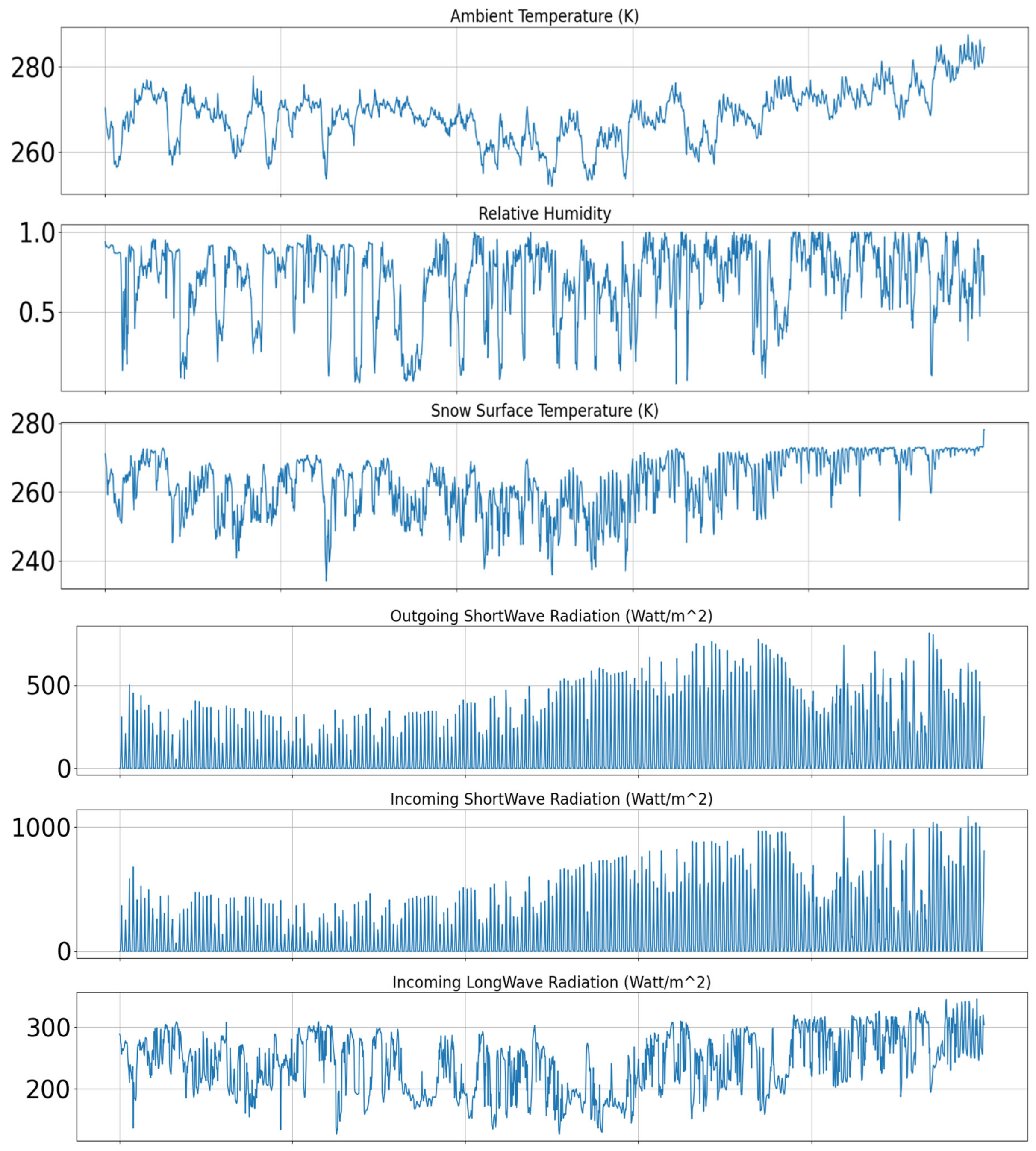
The dataset representing series $W_1,W_2,\dots .,W_T$ was included with the software package of SNOWPACK model, it was collected using an automatic weather station situated at a well known study site Weissfluhjoch (latitude and longitude 46.831 and 9.81 respectively, altitude 2540m a.s.l) located in Davos, Switzerland. The dataset is provided by the WSL-Institute for Snow and Avalanche Research SLF, in this dataset, a data-vector was provided at uniform interval 30 minutes through the entire duration from 30-September-1995 00:30:00 hours till 17-June-1996 00:00:00 hours. Some of the meteorological parameters collected from the AWS at Weissfluhjoch in the duration mentioned above are visualized in Appendix A.

2.4. Model Training and Validation

A dataset for modelling is composed of three time-series denoted by $S_1,S_2,\dots .,S_T$ (snow-surface data); $W_1,W_2,\dots .,W_T$ (meteorological data) and $W_1^{\text{'}},W_2^{\text{'}},\dots .,W_T^{\text{'}}$(estimates of meteorological data) as described in section 2.3. We have generated the series $W_1^{\text{'}},W_2^{\text{'}},\dots .,W_T^{\text{'}}$ and $S_1,S_2,\dots .,S_T$ by simulation program that takes a measured series $W_1,W_2,\dots .,W_T$ and a parameter $\eta \ge 0$ as input (ref section 2.3). Different datasets were generated using a fixed weather series $W_1,W_2,\dots .,W_T$ and varying values of parameter $\eta$. Each dataset (corresponding to a different value of $\eta$) comprised of three time-series $S_1,S_2,\dots .,S_T,$ $W_1,W_2,\dots .,W_T$ and $W_1^{\text{'}},W_2^{\text{'}},\dots .,W_T^{\text{'}}$, representing a different situation encountered in practice. The simulated series $S_1,S_2,\dots .,S_T$ and $W_1^{\text{'}},W_2^{\text{'}},\dots .,W_T^{\text{'}}$ depend on parameter $\eta$, whereas the series $W_1,W_2,\dots .,W_T$ represents the measured data, it is constant in all simulated datasets. The details of generating $W_t^{\text{'}}$ (from $W_t$) are given in Appendix C, details of generating $S_t$ (from $W_t$) are given in Appendix B.

A dataset composed of the three time-series cannot be used to train and validate a ridge regression model, certain pre-processing needs to be done with this dataset. Ridge regression model (section 2.2) requires a set of data points of form $(X_t,y_t)$; here each $X_t$ is a data vector consisting of variables used to predict the target scalar value $y_t$. Since we intend to predict the terms in series $W_t$ from series $W_t^{\text{'}}$ and $S_t$ (section 2.3), the predictor data vectors $X_t$ are derived from series $W_t^{\text{'}}$ and $S_t$, while the target variable $y_t$ is derived from vectors $W_t$ ($y_t$ is taken as a component of vector $W_t$).

We express $X_t$ as:

$$X_t=\left(S_t,S_{t+1}-S_t,W_t^{\text{'}}\right)$$

(2.4.1)

$X_t$ is therefore formed by joining the components of vectors $S_t,$ $S_{t+1}-S_t$ and $W_t^{\text{'}}$ in the above mentioned order.$S_t$ provides information about the present (at time $t$) snow-surface state, $S_{t+1}-S_t$ provides information about the rate of change and $W_t^{\text{'}}$ gives the weather estimate information.

The scalar target $y_t$ will be a meteorological variable we wish to predict at measurement location of snow surface states (point $P$ ). Since each such meteorological variable is a component of vector $W_t$, $y_t$ is therefore equal to a component of $W_t$ i.e $y_t=W_t^{\left(j\right)}$, where $W_t^{\left(j\right)}$ denotes the $j^{th}$ component of vector $W_t$. A training dataset used to predict the $j^{th}$ component can be expressed in terms of time-series as $\left(X_1,W_1^{\left(j\right)}\right),\left(X_2,W_2^{\left(j\right)}\right),\dots .,(X_{T-1},W_{T-1}^{\left(j\right)})$, where $W_t^{\left(j\right)}$ denotes the $j^{th}$ component of vector $W_t$, $X_t$ is defined by equation 2.4.1.

We will denote the dataset $\left(X_1,W_1^{\left(j\right)}\right),\left(X_2,W_2^{\left(j\right)}\right),\dots .,(X_{T-1},W_{T-1}^{\left(j\right)})$ by $D_j^{\eta }$, where $\eta \ge 0$ is the parameter input to the generating simulation for $W_1^{\text{'}},W_2^{\text{'}},\dots .,W_T^{\text{'}}$ and $S_1,S_2,\dots .,S_T$. This notation expresses the dependence of the dataset on the parameter $\eta$ and the target variable ($j$) it represents. A separate kernel ridge regression model with radial basis function kernel was trained for each simulated dataset $D_j^{\eta }$, 80% of points were sampled randomly for training and the remaining 20% were used for testing. For any parameter $j$, we generate the datasets $D_j^{\eta }$ for certain fixed values of parameter $\eta$, then training and compiling the model performance on each dataset is done. We have visualized our results in Appendix D, the model performance was measured using the co-efficient of determination and the mean absolute error.

We have also tried to understand the effect of estimates $W_t^{\text{'}}$ on model performance, for each dataset we use to train and validate a model, we also generate a corresponding dataset with the weather estimates $W_t^{\text{'}}$ removed. The removal of weather parameters is achieved by setting the components of $W_t^{\text{'}}$ to zero in each vector $X_t$ (eq. 2.4.1) of the dataset, this removes all information contained in the estimates for that dataset. The results for all scenarios have been visualized in Appendix D and discussed Section 3.

3. Results and Discussion

Snow surface microstructure is constantly changing due to changes in meteorological conditions near it. We try to analyze if it is possible to deduce the meteorological parameters from changes in snow-surface, a simulation based approach has been utilized due to economic reasons. A dataset representing certain actual scenario is first generated using a simulation (refer section 2.3), we train and validate a kernel ridge regression model on this generated dataset. Simulated scenarios depend on a parameter $\eta$ representing snow-surface data quality, each scenario also considers the availability or non-availability of certain meteorological estimate data. Table A3 and Table A4 show the results obtained when a model is trained and validated on datasets representing these scenarios, we have simulated datasets for values of $\eta =0.0,0.1,0.2,0.3$, for each $\eta$ we have also considered the scenario when the meteorological estimates are not-available.

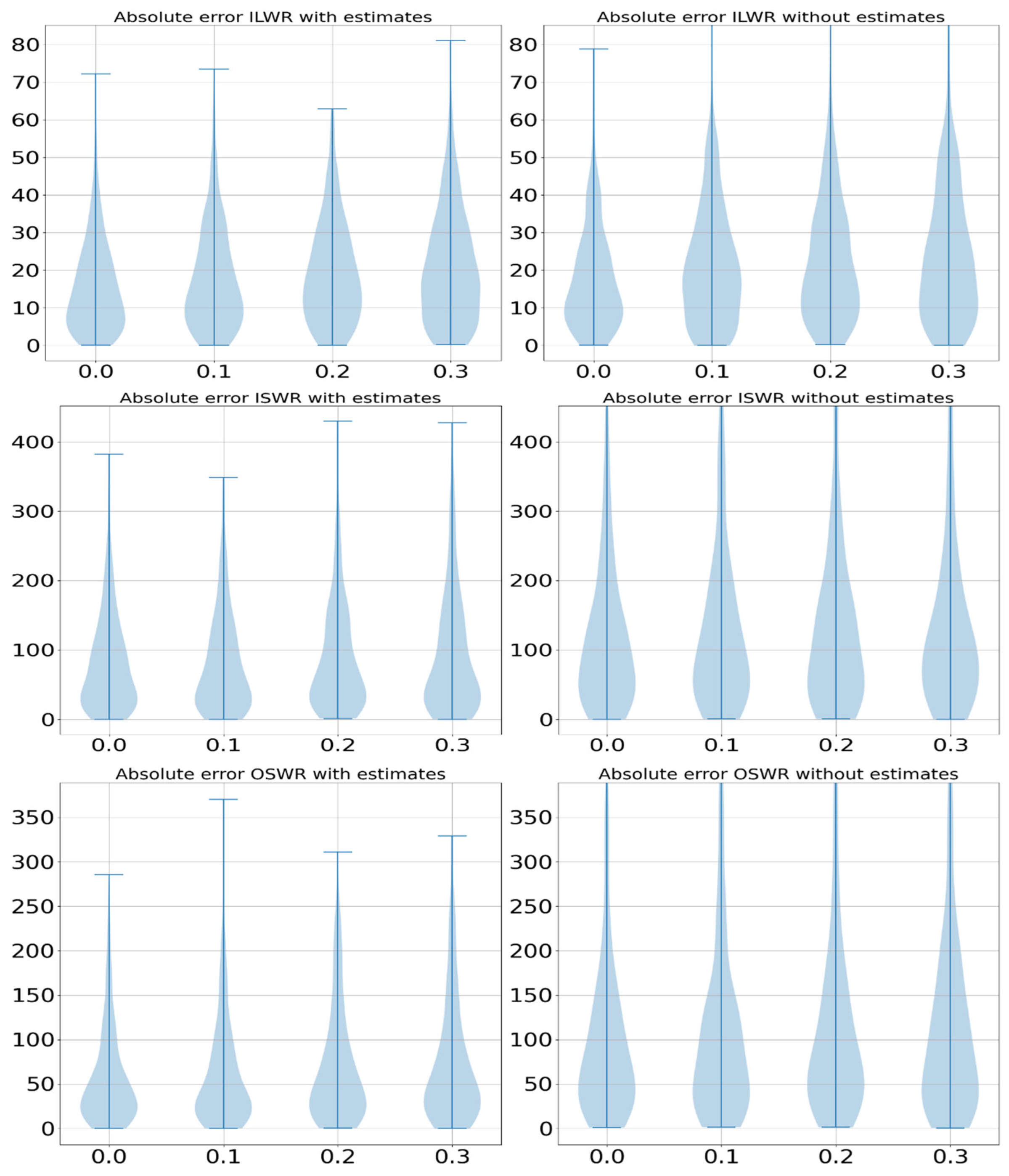
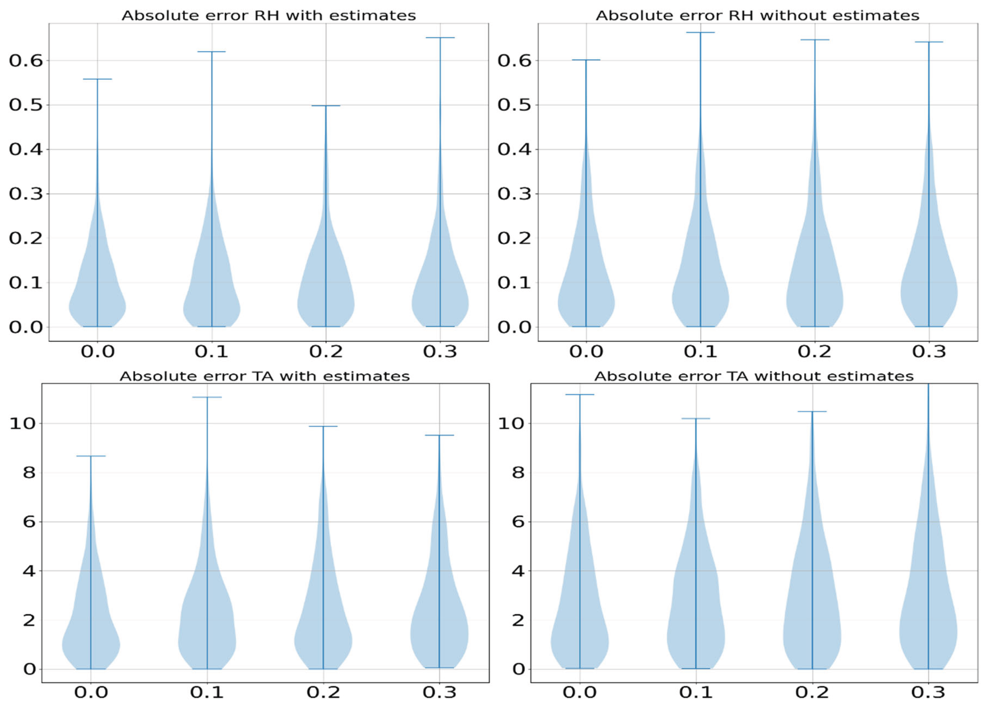
Table A3 shows a decreasing trend in co-efficient of determination (for all parameters) for increasing values of $\eta$. Similarly in Table A4 we see an increasing trend in mean absolute error (for all parameters) for increasing values of $\eta$. The results also show a strong dependence on meteorological estimates, in datasets representing scenarios where these estimates are unavailable we see significant performance drop. (Table A3 and Table A4) show that Relative Humidity and Outgoing Shortwave Radiation are highly dependent on availability of estimates, however Incoming Longwave Radiation and Ambient Temperature are relatively unaffected. Figure A2 shows the dependence of mean absolute error on parameter $\eta$ and the availability of weather estimates.

The simulation process was designed so that the model performance on actual data is likely to be much higher than on the simulated datasets (refer Section 2.3). When accounting for this performance under-estimation, results of Table A3 suggest an acceptable performance level (for scenarios where estimates are available) for all parameters except Relative Humidity. In scenarios where meteorological estimates are unavailable, no parameter shows an acceptable performance level.

The parameters: sphericity, dendricity, co-ordination number, bond size, grain size were used to represent snow-surface microstructure in our datasets (Table A2). Detailed images of snow-microstructure are obtained using x-ray tomography, since these parameters characterize snow micro-structure, they can be inferred using detailed tomography image data. Conventional tomography equipment is very expensive to deploy in field and requires manual effort to operate. However we only need the snow-surface microstructure in our datasets, detailed images of surface micro-structure can be obtained using high resolution cameras located above the snow surface. Since our model only requires data of surface, a high resolution camera may provide the required snow-surface microstructure data at low cost.

The measurement of surface micro-structure parameters used in this study maybe difficult using the camera, however the information provided by the detailed surface images will include the information that these parameters provide. We may assume that in actual practice the information from such images is much greater than contained in these parameters (sphericity, dendricity, co-ordination number, bond size, grain size ), therefore using the image data is likely to result in much higher performance than our results using simulated data suggest.

4. Conclusions and Future Work

Snow surface changes continuously due to changes in weather, SNOWPACK and CROCUS are complex deterministic models that map the meteorological parameters to changes in snowcover microstructure. In this work we try to understand if it is possible to reverse this mapping: we try to recover meteorological parameters from changes in snowcover surface. We were able to deduce meteorological parameters from certain snow-surface microstructural parameters if an estimate of these meteorological parameters is known. We were able to get reasonable results without needing accurate estimates.

We have used a simulation approach, certain precautions are therefore required when generalizing these results to actual field conditions. We try to ensure that simulated datasets we use contain less information than the datasets we are likely to encounter in practice, therefore the model performance on these datasets is also expected to be lower than actual datasets. The results we have obtained can be interpreted as lower bounds on actual results that maybe expected in practice, they suggest promising potential of our approach using actual data.

Our approach also relies on measurement of certain micro-structural parameters of snow, conventionally detailed microstructural measurements require tomographic images of snow. However tomography is not a feasible measurement method in field conditions, since we only require micro-structure of snow surface in our approach, a high resolution camera can be used to get snow surface images containing detailed data of micro-structure. Conclusions of our work likely apply to models using these images because they also contain all the information contained in the microstructure parameters used in our study (however the modelling approach may require some changes to use this data).

We propose two practical applications of these results here, however we have not explored them in great detail. The additional information in snowcover surface, if measured economically can be used to optimize weather measurement systems. Weather is usually measured by a grid of automatic weather systems, our model can be used to infer meteorological parameters at locations where automatic weather stations are at considerable distance. The data from other weather stations in grid can be combined with snow-surface data of a location to get weather parameters at the location using our approach. This reduces the instrumentation at the location and therefore the cost involved in measurement (refer Appendix E for details). Another potential application is in the down-scaling of outputs from numerical weather prediction models, since snow-surface microstructure includes information about weather it maybe used as an additional input to numerical models to improve their accuracy.

There are several directions for future work, implementation and validation of the approach in field is the most important. Another direction is to numerically model the inversion of surface micro-structure to the meteorological parameters, such numerical models eliminate the need for large datasets used by machine learning models. Including the information in snow surface microstructure to improve numerical weather prediction and weather interpolation models can also be an important future research direction.

References

1. Barnett, T. P.; Dümenil, L.; Schlese, U.; Roeckner, E. The effect of Eurasian snow cover on global climate. Science 1988, 239(4839), 504–507. [Google Scholar] [CrossRef] [PubMed]
2. Bartelt, P.; Lehning, M. A physical SNOWPACK model for the Swiss avalanche warning: Part I: numerical model. Cold Regions Science and Technology 2002, 35(3), 123–45. [Google Scholar] [CrossRef]
3. Boyarskii, D. A.; Tikhonov, V. V. The influence of stratigraphy on microwave radiation from natural snow cover. Journal of electromagnetic waves and applications 2000, 14(9), 1265–1285. [Google Scholar] [CrossRef]
4. Brun, E.; David, P.; Sudul, M.; Brugnot, G. A numerical model to simulate snowcover stratigraphy for operational avalanche forecasting. J. Glaciol. 1992, 38 128, 13–22. [Google Scholar] [CrossRef]
5. Cohen, J.; Rind, D. The effect of snow cover on the climate. J. Climate 1991, 4, 689–706. [Google Scholar] [CrossRef]
6. Coléou, C.; Lesaffre, B.; Brzoska, J.-B.; Ludwig, W.; Boller, E. Three-dimensional snow images by X-ray microtomography; Ann. Glaciol., Jan 2001; vol. 32, pp. 75–81. [Google Scholar] [CrossRef]
7. Gay, M.; Fily, M.; Genthon, C.; Frezzotti, M.; Oerter, H.; Winther, J.-G. Snow grain-size measurements in Antarctica; J. Glaciol., Jan 2002; vol. 48, no. 163, pp. 527–535. [Google Scholar] [CrossRef]
8. Hastie, T.; Tibshirani, R.; Friedman, J. The Elements of Statistical Learning, 2nd edition; Springer, 2009; pp. 61–69. [Google Scholar]
9. Johnson, J. B.; Schneebeli, M. Characterizing the microstructural and micromechanical properties of snow. Cold Reg. Sci. Technol. 1999, 30(1–3), 91–100. [Google Scholar] [CrossRef]
10. Lehning, M.; Bartelt, P.; Brown, B.; Fierz, C.; Satyawali, P. A physical SNOWPACK model for the Swiss avalanche warning. Part II: snow microstructure. Cold Reg. Sci. Technol. 2002, 35, 147–167. [Google Scholar] [CrossRef]
11. Lehning, M.; Völksch, I.; Gustafsson, D.; Nguyen, T. A.; Stähli, M.; Zappa, M. ALPINE3D: a detailed model of mountain surface processes and its application to snow hydrology. Hydrological Processes: An International Journal 2006, 20(10), 2111–2128. [Google Scholar] [CrossRef]
12. Lesaffre, B.; Pougatch, E.; Martin, E. Objective determination of snow-grain characteristics from images; Ann. Glaciol., Jan 1998; vol. 26, pp. 112–118. [Google Scholar] [CrossRef]
13. Mohri, M.; Rostamizadeh, A.; Talwakar, A. Foundations of machine learning; MIT Press, 2012; pp. 89–116. [Google Scholar]
14. Morin, S.; Horton, S.; Techel, F.; Bavay, M.; Coléou, C.; Fierz, C.; Vionnet, V. Application of physical snowpack models in support of operational avalanche hazard forecasting: A status report on current implementations and prospects for the future. Cold regions science and technology 2020, 170, 102910. [Google Scholar] [CrossRef]
15. Schirmer, M.; Lehning, M.; Schweizer, J. Statistical forecasting of regional avalanche danger using simulated snowcover data. Journal of Glaciology 2009, 55(193), 761–768. [Google Scholar] [CrossRef]
16. Schaffhauser, A.; Adams, M.; Fromm, R.; Jörg, P.; Luzi, G.; Noferini, L.; Sailer, R. Remote sensing based retrieval of snow cover properties. Cold Regions Science and Technology 2008, 54(3), 164–175. [Google Scholar] [CrossRef]
17. Schweizer, J.; Kronhoml, K.; Jamieson, J.B.; Birkeland, K.W. Rewiew of spatial variability of snowpack properties and its importance for avalanche formation; Cold Regions Science and Technology, 2008; Volume 51, pp. 253–272. [Google Scholar] [CrossRef]
18. Thackeray, C. W.; Derksen, C.; Fletcher, C. G.; Hall, A. Snow and climate: Feedbacks, drivers, and indices of change. Current Climate Change Reports 2019, 5, 322–333. [Google Scholar] [CrossRef]
19. Vavrus, S. The role of terrestrial snow cover in the climate system. Climate Dynamics 2007, 29, 73–88. [Google Scholar] [CrossRef]
20. Viallon-Galinier, L.; Hagenmuller, P.; Reuter, B.; Eckert, N. Modelling snowpack stability from simulated snow stratigraphy: Summary and implementation examples. Cold Regions Science and Technology 2022, 201, 103596. [Google Scholar] [CrossRef]
21. Woods, R. A. Analytical model of seasonal climate impacts on snow hydrology: Continuous snowpacks. Advances in water resources 2009, 32(10), 1465–1481. [Google Scholar] [CrossRef]
22. Xiao, X.; He, T.; Liang, S.; Zhao, T. Improving fractional snow cover retrieval from passive microwave data using a radiative transfer model and machine learning method. IEEE Transactions on Geoscience and Remote Sensing 2021, 60, 1–15. [Google Scholar] [CrossRef]
Disclaimer/Publisher’s Note: The statements, opinions and data contained in all publications are solely those of the individual author(s) and contributor(s) and not of MDPI and/or the editor(s). MDPI and/or the editor(s) disclaim responsibility for any injury to people or property resulting from any ideas, methods, instructions or products referred to in the content.
Copyright: This open access article is published under a Creative Commons CC BY 4.0 license, which permit the free download, distribution, and reuse, provided that the author and preprint are cited in any reuse.