
Submitted:
09 May 2026
Posted:
11 May 2026
You are already at the latest version
Abstract
Addressing the issues of insufficient adaptability and limited energy efficiency optimization capabilities in traditional tunnel lighting control methods under complex traffic conditions, this paper proposes a dynamic dimming strategy for tunnel lighting based on the Proximal Policy Optimization (PPO) algorithm.First, the tunnel lighting system is modeled as a reinforcement learning environment. A state space integrating multi-dimensional information—including traffic flow, vehicle speed, external brightness, and tunnel section location—is constructed, and a continuous action space is designed to enable precise dimming control for each functional section. Based on this, a multi-objective reward function is established that integrates brightness tracking error, energy consumption optimization, control stability, and environmental adaptability to guide the agent in learning the optimal dimming strategy.Subsequently, model training and experimental validation were conducted using actual tunnel operation data.Experimental results indicate that, compared to traditional L20 control strategies, the proposed method achieves smoother brightness regulation and higher zone control accuracy while ensuring driving safety and visual comfort, and demonstrates significant energy-saving advantages during periods of high lighting demand. In summary, the dynamic dimming strategy based on the PPO algorithm shows promising application prospects and engineering value in intelligent tunnel lighting systems.
Keywords:
tunnel lighting
; reinforcement learning
; PPO algorithm
; dynamic dimming
; energy-saving optimization
1. Introduction
With the continuous improvement of China’s transportation infrastructure, the number of highway tunnels has been steadily increasing, and tunnel lighting systems are playing an increasingly important role in ensuring driving safety and enhancing driving comfort. Proper lighting control can not only effectively alleviate the visual discomfort drivers experience due to sudden changes in brightness at tunnel entrances and exits but also help reduce the risk of traffic accidents. At the same time, against the backdrop of the “dual carbon” goals, the issue of energy consumption in tunnel lighting systems has garnered increasing attention. How to achieve energy-saving optimization while ensuring lighting safety has become a key research direction in the field of intelligent tunnel lighting.
Domestic research on highway tunnel lighting control has trended from traditional control toward intelligent methodologies. Early studies predominantly utilized classical control theory. Du et al. [1] developed a fuzzy PID-based control system that established mapping relationships between external luminance and sectional safety luminance through segmented modeling to implement dynamic dimming. While structurally simple and stable, such methods exhibit limited adaptability to complex environments. Consequently, research has expanded into multi-factor coupling and intelligent optimization. Miao et al. [2] integrated color temperature with traditional luminance adjustment, using neural networks to build intelligent dimming models for integrated light environment regulation at tunnel portals. With the rise of artificial intelligence, data-driven methods have gained prominence. Hu et al. [3] formulated tunnel lighting control as a Markov Decision Process (MDP) and applied deep reinforcement learning for autonomous dimming strategy acquisition, ensuring safety while minimizing energy use. Overall, domestic research has evolved from rule-driven to data-driven paradigms, yet gaps remain in unified multi-factor modeling and engineering adaptability.
Research in the field of tunnel lighting control began earlier abroad, with a focus on system integration, intelligent control, and human-centered optimization. At the system level, Yong et al. [4] developed an on-demand lighting control system based on IoT technology, achieving networked and intelligent management of the lighting system by integrating traffic forecasts with multi-source information. In terms of control methods, R et al. [5] established a dimming model based on a backpropagation (BP) neural network. By combining traffic flow prediction with closed-loop control, they achieved continuous dimming and introduced an energy consumption monitoring mechanism, significantly reducing system energy consumption. Suying et al. [6] utilized ambient light ratios and principal component analysis to achieve adaptive brightness adjustment driven by multi-source data. In recent years, research has further evolved toward deep learning and human-centered approaches. Liu et al. [7] constructed a luminance demand prediction model based on attention mechanisms and dual LSTMs, integrating multiple factors such as ambient light, traffic flow, and vehicle speed to achieve high-precision predictions. They optimized the lighting transition process through segmented interpolation, thereby enhancing drivers’ visual adaptability. Overall, international research is relatively mature in terms of system integration and the application of intelligent algorithms, and it also takes drivers’ visual needs into account in a more systematic manner.
In summary, research on tunnel lighting control has progressively transitioned from traditional rule-based methods to AI-driven approaches, making notable strides in enhancing both lighting safety and energy efficiency. While domestic studies primarily focus on the optimization of control strategies and the application of novel algorithms, international research delves deeper into system integration, multi-source information fusion, and human-centric modeling. Despite these advancements, current methods still exhibit limitations in multi-factor collaborative modeling, adaptability to complex environments, and operational stability in engineering applications. Furthermore, the systematic characterization of the driver’s visual adaptation process remains inadequate. Therefore, it is imperative to further develop high-precision, multi-factor coupled intelligent lighting control methods tailored to practical scenarios, ultimately achieving the synergistic optimization of lighting safety and energy efficiency.
2. Materials and Methods
2.1. Continuous Modeling Methods for Discrete Lighting Parameters
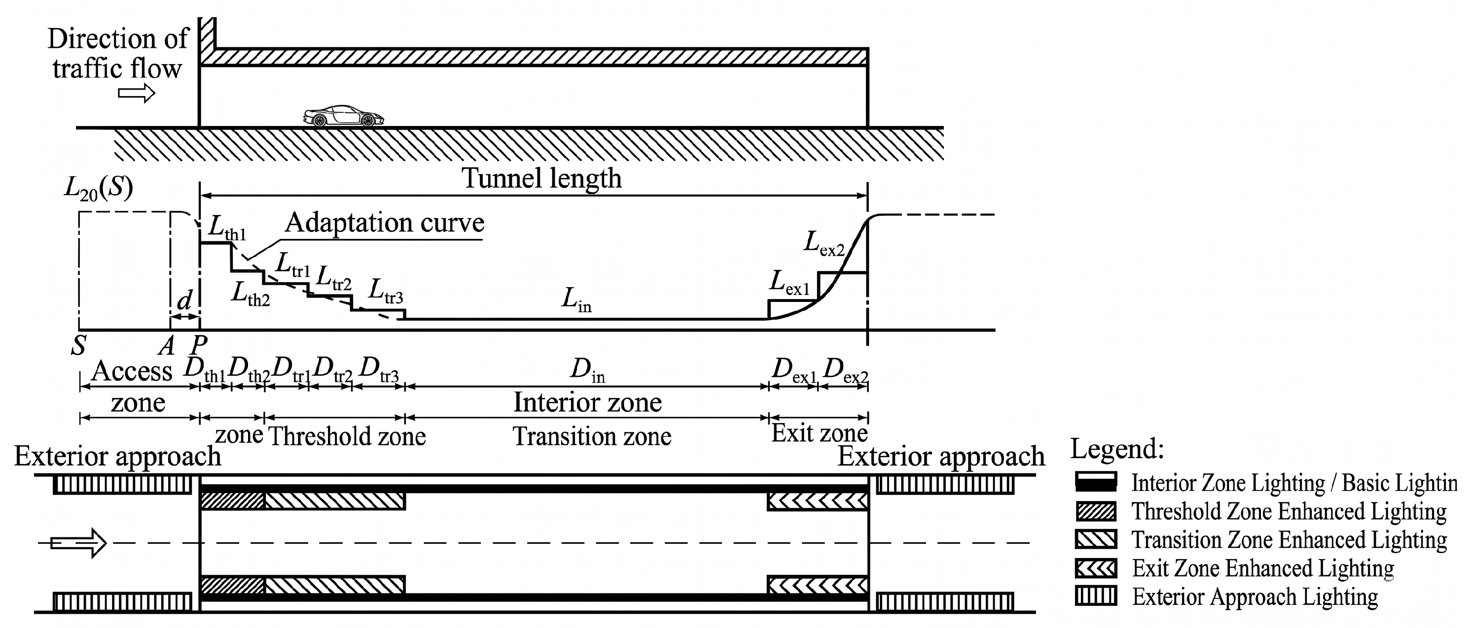
There are significant differences between the lighting environments inside and outside tunnels. When a vehicle enters or exits the portal area, the driver’s visual system must rapidly transition from light adaptation to dark adaptation, and then from dark adaptation back to light adaptation, within a short period of time.If the longitudinal luminance distribution within the tunnel is improperly designed, it can easily lead to reduced target recognition capability in the portal area, thereby adversely affecting driving safety. Therefore, tunnel lighting design typically follows the principles of driver visual adaptation, arranging the longitudinal lighting environment into distinct zones rather than employing a uniform luminance throughout the entire tunnel.
According to the "Detailed Rules for Highway Tunnel Lighting Design," tunnel lighting is generally divided into entrance, transition, intermediate, and exit sections, with the illuminance levels of each section corresponding to different visual functions and operational requirements. Among these, the entrance section is most significantly influenced by external brightness and traffic conditions; its target illuminance not only directly affects the driver’s visual safety during the initial entry into the tunnel but also largely determines the system’s overall energy consumption.Based on this, this paper first conducts a continuous modeling study on the illuminance parameters of the entrance section.
Figure 1.
Reward Variation Curve During PPO Training.
2.1.1. Continuous Modeling of Target Illuminance for the Entrance and Transition Sections
According to the "Detailed Rules for Highway Tunnel Lighting Design," the entrance section is typically divided into two lighting zones, th1 and th2, with the corresponding illuminance formulas as follows:
In these equations, and denote the target illuminance levels for the two lighting zones in the tunnel entrance section, respectively. represents the illuminance outside the tunnel, and k is the illuminance reduction factor for the entrance section.
As shown in Table 1, the luminance reduction coefficient k is typically selected based on the design-hour traffic volume and design speed. This method is suitable for parameter determination during the engineering design phase and offers the advantages of simplicity and clear boundaries. However, under actual operating conditions, traffic flow and vehicle speeds exhibit continuous variation. If fixed-tier parameters are still used, it is difficult to meet the requirements of smart tunnel lighting systems for real-time, continuous, and refined control.
As shown in Table 1, the entrance section brightness reduction coefficient k is influenced by both the design speed and the design hourly traffic volume; moreover, the pattern of its variation with speed differs across different traffic volume ranges. To balance model continuity, engineering feasibility, and compliance with standards, this paper uses the values recommended by the standards as discrete anchor points to perform a continuous reconstruction of the variation pattern of k. Specifically, traffic conditions are divided into three categories: high-traffic zones, low-traffic zones, and intermediate transition zones. In the high-traffic and low-traffic zones, boundary functions for k with respect to vehicle speed v are established, respectively; in the intermediate transition zone, a continuous expression for is constructed through traffic-weighted interpolation, thereby achieving dynamic adjustment of the reduction coefficient in response to changes in traffic volume and vehicle speed.
Based on the above modeling approach, this paper employs nonlinear least squares regression to fit the discrete data from the specifications, deriving analytical expressions for k as a function of vehicle speed v under both high-traffic and low-traffic conditions. Taking a one-way traffic scenario as an example, the luminance reduction coefficient for the entrance section can be expressed as:
High-traffic conditions ():
Low-traffic conditions ():
For the intermediate adjustment range , a linear weighted interpolation model based on boundary functions is adopted, utilizing the above two boundary equations for real-time calculation:
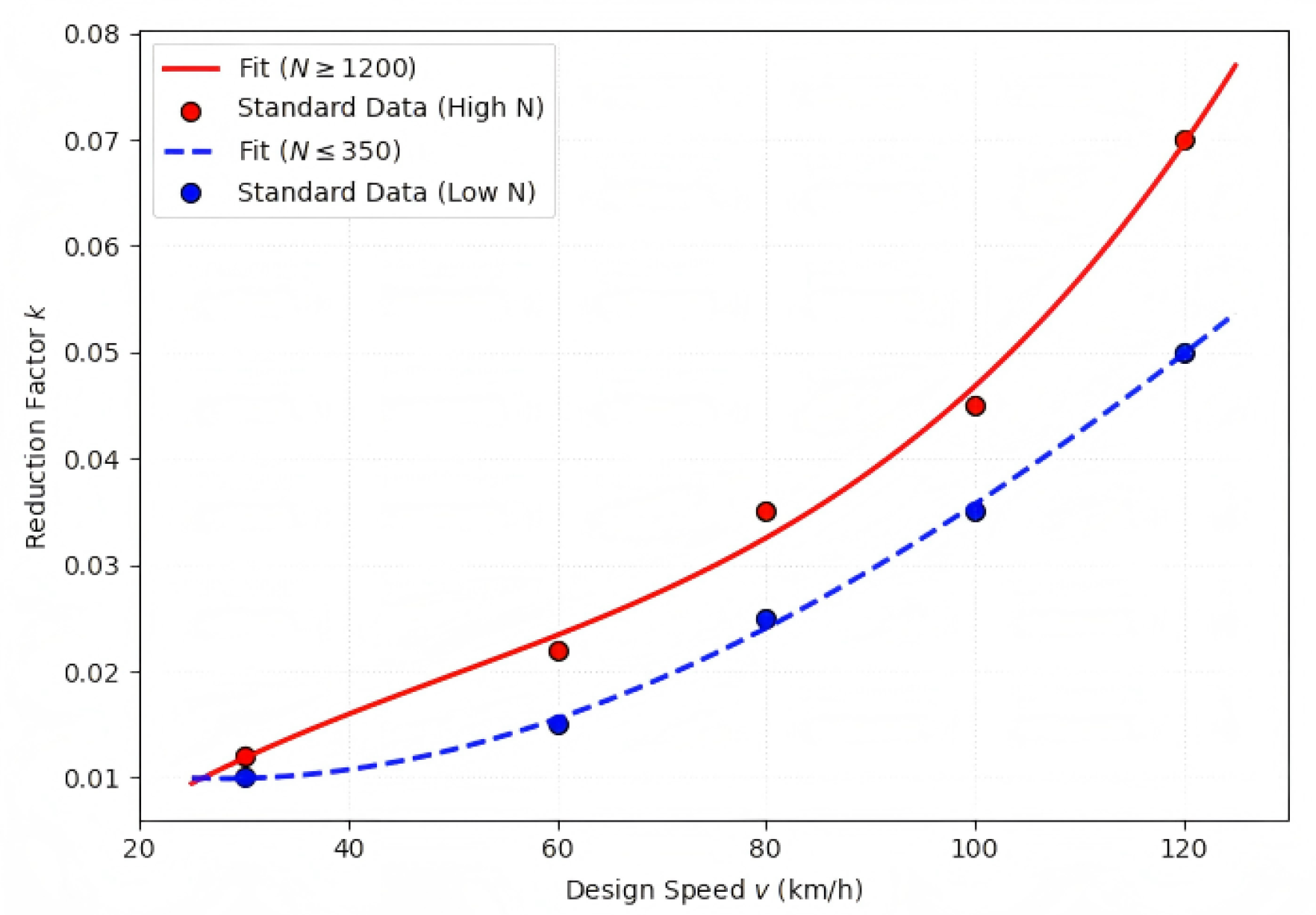
In these equations, v is the vehicle operating speed, and N is the design hourly traffic volume. Verification through residual analysis shows that the established model exhibits good fitting accuracy under both high- and low-traffic conditions, with the mean squared error controlled within the order of magnitude of . This indicates that the fitted curve effectively captures the variation patterns reflected in the standard discrete data.
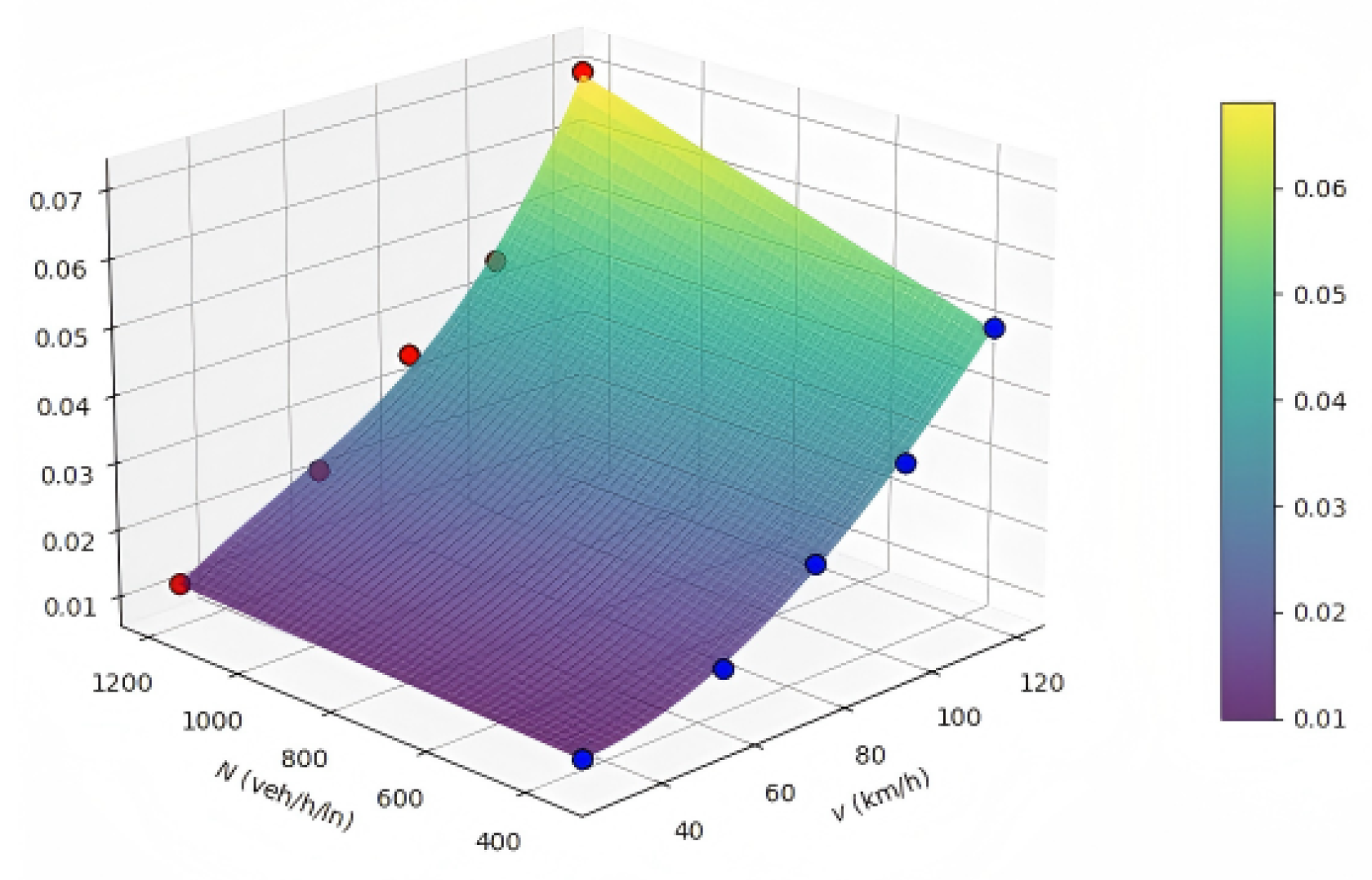
Figure 2 compares the fitted curves with the standard discrete data points under both high- and low-traffic conditions. It can be seen that the fitted curve shows good consistency with the original discrete data points, accurately capturing the basic trend of how the brightness reduction coefficient at the entrance section varies with vehicle speed under these two boundary conditions. Figure 3 displays the continuous surface formed by k as a function of vehicle speed and traffic volume within the intermediate transition zone. It can be observed that as vehicle speed increases, the reduction coefficient exhibits an overall upward trend; under the same vehicle speed conditions, an increase in traffic volume also leads to a corresponding increase in k. This indicates that the target brightness of the entrance section should be dynamically adjusted according to changes in traffic conditions, and the continuous model can provide smooth and computable parameter support for this process.
Figure 2.
Fitting results under high- and low-traffic conditions.
According to the “Detailed Rules for the Design of Highway Tunnel Lighting,” the transition section is divided into three lighting zones—tr1, tr2, and tr3—based on the principle of gradual reduction. The formula for calculating the luminance is:
Figure 3.
Continuous surface of k in the intermediate transition zone.
As can be seen, the target luminance of the transition section is directly determined by the first-level luminance of the entrance section. Therefore, when the luminance reduction coefficient k for the entrance section is dynamically adjusted through continuous modeling, the target luminance levels of the transition section can also be continuously updated accordingly, thereby ensuring the coordination and continuity of the luminance transition between the entrance section and the transition section.
2.1.2. Continuous Modeling of Target Illuminance for the Intermediate and Exit Sections
To enable the target luminance of the intermediate section to adapt to real-time adjustment requirements under continuous traffic conditions, this paper performs a continuous reconstruction of the intermediate section’s luminance parameters based on the recommended values in Table 2 of the standard. Consistent with the continuous modeling of the entrance section’s luminance reduction coefficient k—that is, using the standard’s discrete values as safety anchors—a target luminance function for the intermediate section is constructed to accommodate continuous changes in vehicle speed and traffic volume, while preserving the luminance levels at key design nodes. This approach does not replace the code requirements but establishes a continuous reference model within the code’s recommended range that is better suited for real-time optimization control. It aims to avoid the luminance step effects caused by traditional stepwise control and provides smooth target inputs for subsequent model predictive control.
Given the step-like distribution of the intermediate segment luminance in Table 2, this paper employs a high-order polynomial regression algorithm to ensure continuity. Boundary functions for with respect to vehicle speed v are constructed separately for high-traffic and low-traffic conditions, and linear weighted interpolation is used to achieve a continuous transition in luminance within the intermediate traffic range:
High-traffic conditions ():
Low-traffic conditions ():
For the scenario, a linear weighted interpolation model based on boundary equations is also used:
In these equations, and represent the luminance of the intermediate section under high-traffic and low-traffic conditions, respectively.
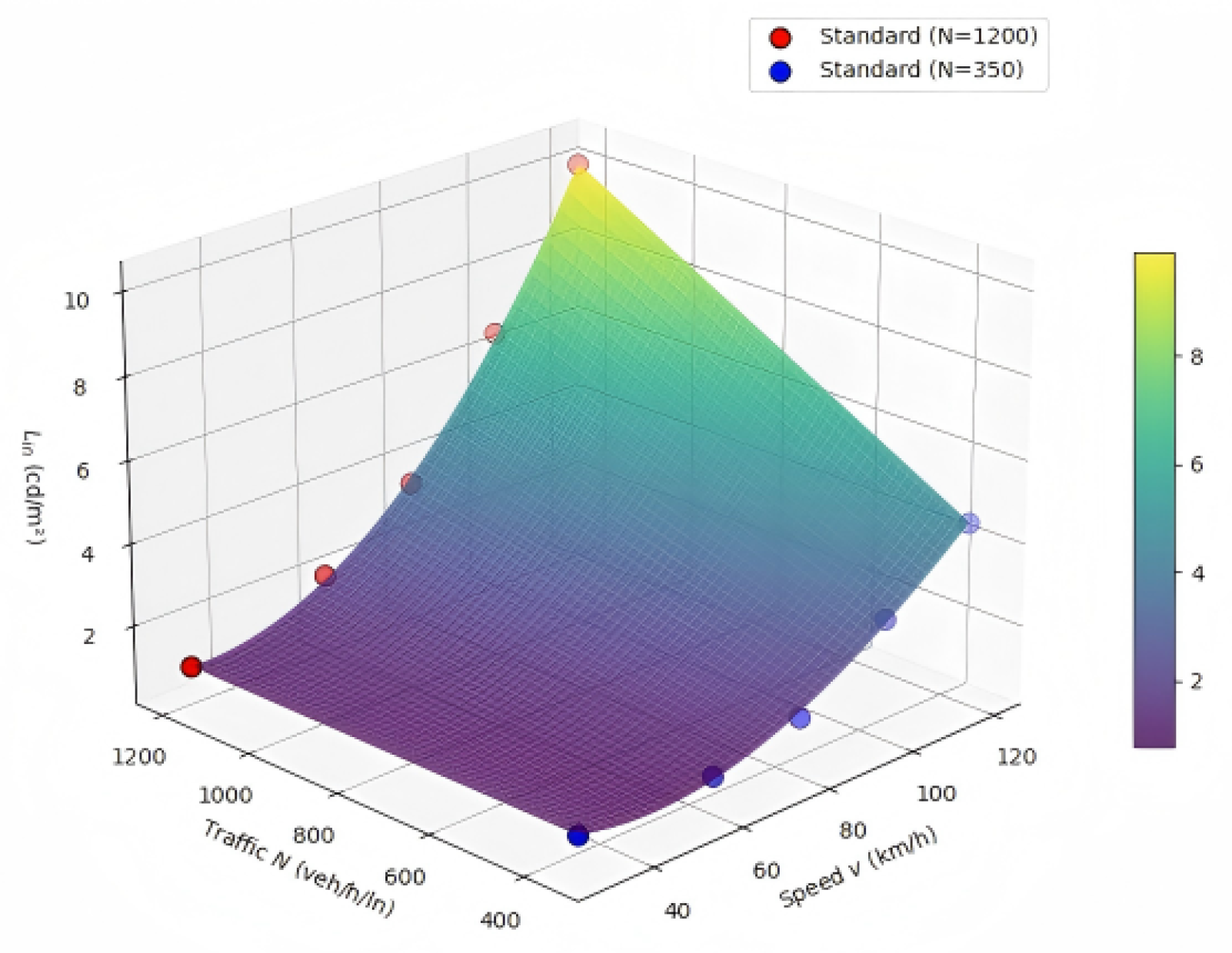
Verification of fitting accuracy confirms that the proposed continuous model for intermediate section luminance fits the standard discrete data well and maintains reasonable variation trends across the entire speed range.Figure 4 compares the fitted curves of intermediate section luminance under high- and low-traffic conditions with the standard discrete data. The curves show good consistency with the discrete points, capturing the basic trend of luminance variation with vehicle speed under the two boundary conditions. Figure 5 presents the continuous surface of intermediate section luminance as a function of vehicle speed and traffic volume in the intermediate traffic range. As shown, for a given traffic volume, target luminance increases with rising vehicle speed; for a given speed, target luminance also rises with increasing traffic volume. These results indicate that intermediate section lighting requirements are strongly dependent on operating conditions, requiring dynamic adjustment according to real-time traffic conditions.
Figure 4.
Fitting results of under high- and low-traffic conditions.
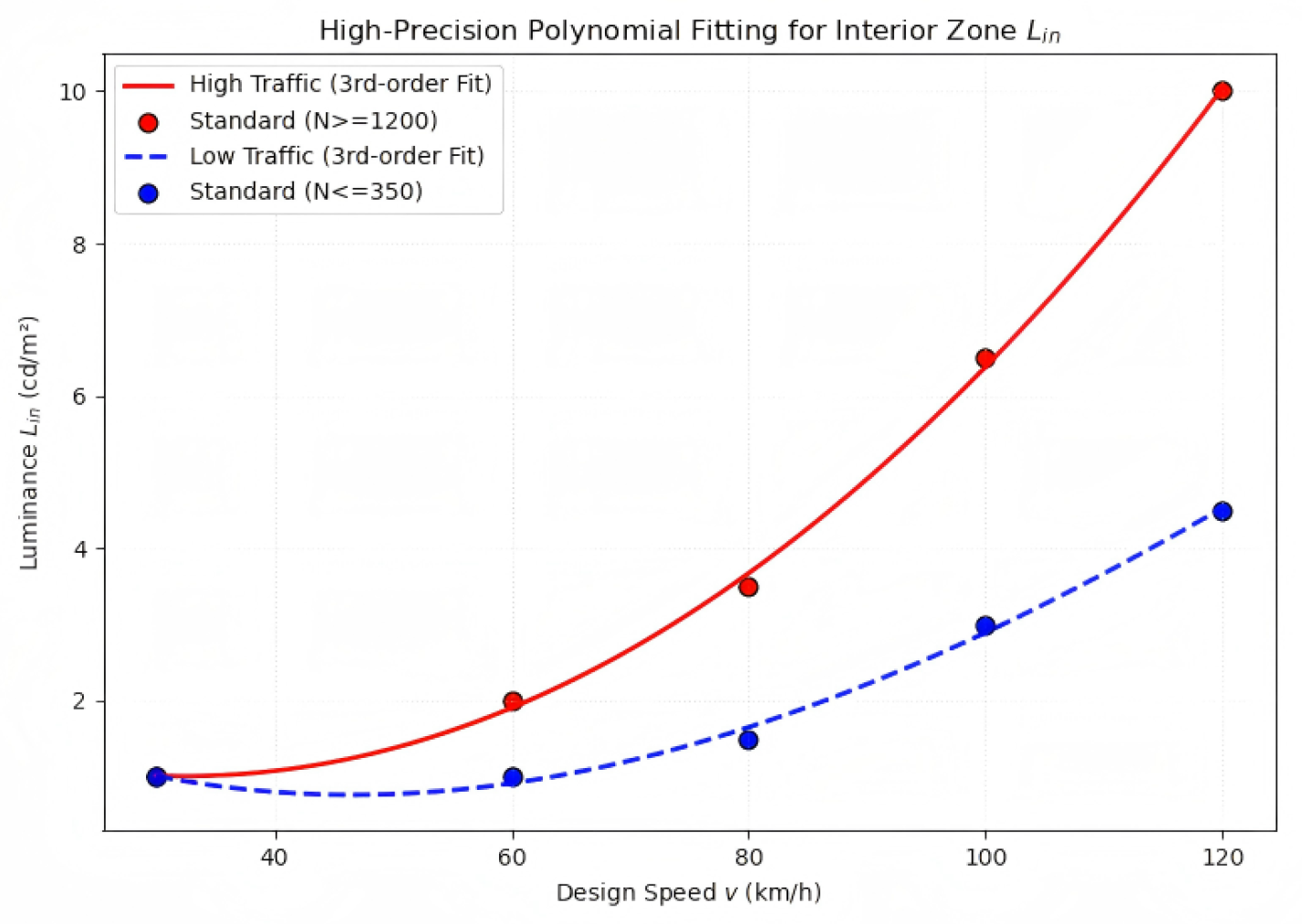
Figure 5.
Continuous surface of intermediate section luminance.
Once the target luminance for the intermediate section is obtained, the luminance for the exit section can be further determined based on the specified relationships. According to the “Detailed Rules for the Design of Highway Tunnel Lighting,” the exit section is divided into two lighting zones, ex1 and ex2, with the corresponding luminance formulas as follows:
The target illuminance of the exit section is directly related to that of the intermediate section. Once the illuminance of the intermediate section is dynamically updated via the continuous model, the illuminance of the exit section can also be adjusted synchronously in response to changes in traffic conditions, thereby ensuring consistency in the illuminance transition between the intermediate and exit sections. This modeling approach enables the continuous generation of target illuminances for the entrance, transition, intermediate, and exit sections within a unified framework, laying the foundation for the subsequent development of a multi-section coordinated dimming control model.
2.2. Tunnel Lighting Dimming Strategy Based on the PPO Algorithm
In the design of tunnel lighting systems, dynamic dimming strategies based on reinforcement learning can effectively adapt to variations in traffic flow and ambient lighting conditions, ensuring optimal lighting performance within the tunnel while minimizing energy consumption.To ensure the stable and efficient operation of this strategy in practical applications, this chapter will detail the design of a tunnel lighting dimming strategy based on the PPO algorithm, including the definition of the state space, the design of the action space and dimming decisions, the construction of the reward function, and the design of the training and optimization process.Through these design elements, we can fully leverage the advantages of the PPO algorithm to enable the lighting system to make reasonable dimming decisions in a constantly changing environment, thereby enhancing the system’s intelligence and energy efficiency.
2.2.1. State Space Design
In the problem of tunnel lighting control, the PPO algorithm needs to make dynamic lighting adjustment decisions based on the current environmental state.To effectively define the state space, this study integrates multi-dimensional factors such as traffic conditions inside and outside the tunnel, lighting demands, and historical data. Specifically, the state space includes variables such as traffic density, vehicle speed, external illuminance, and tunnel location, while also accounting for the influence of historical data, thereby ensuring that the reinforcement learning algorithm can make reasonable decisions based on both current and historical environmental states.
(1) Definition of the State Space Assuming that at time t, the state of the tunnel can be represented by the following vector:
In these equations,
- represents the traffic density inside the tunnel, reflecting the number and distribution of vehicles;
- represents the vehicle speed inside the tunnel, which affects the driver’s required visibility range;
- denotes the ambient light intensity outside the tunnel, which affects the adjustment of the tunnel’s lighting intensity;
- is a normalized position variable, representing the relative position of a vehicle within the tunnel, with a range of ;
- is the average traffic density over the past k time steps, representing the long-term trend of traffic conditions;
- is the rate of change in traffic density, reflecting dynamic changes in traffic flow;
- is the average external brightness over the past k time steps, providing the trend of external illumination changes;
- is the rate of change of external brightness, helping the model understand rapid changes in external illumination.
(2) Tunnel Position Modeling To accurately characterize the vehicle position inside the tunnel and adopt normalized position representation, this study divides the total tunnel length into four zones: the entrance section, transition section, intermediate section, and exit section. To ensure the continuity of the position variable, the full tunnel position is normalized to the range of . Using this method, the actual tunnel position is mapped to the normalized variable , which denotes the current relative position of the vehicle.
In the state space design, the normalized position variable is incorporated as an input component, allowing the PPO algorithm to perform adaptive control according to the tunnel section where the vehicle is located. The value range of the position variable is , and its specific definition is given as follows:
Specifically, the range of the position variable and the segment divisions are as follows:
- When , it is the tunnel entrance segment, ;
- When , it is the tunnel transition section, ;
- When , it is the middle section of the tunnel, ;
- When , it is the tunnel exit section, ;
(3) Historical Data Modeling
To improve the model’s sensitivity to variations in traffic flow and illumination, historical data are introduced in this study. Given that the environmental conditions inside and outside the tunnel present inertia and trend characteristics, the instantaneous traffic density, vehicle speed and external brightness cannot fully represent the historical dynamic characteristics of the system. Therefore, the historical data of the past k time steps, including traffic density, vehicle speed and external brightness, are integrated into the state space. These historical data are modeled via statistical features, and the specific definitions are as follows:
: represents the average traffic density over the past k time steps, which is used to capture the long-term trend of traffic flow.
: represents the rate of change of traffic density, reflecting the dynamic variation of traffic conditions.
: represents the average external brightness over the past k time steps, which is used to capture the trend of external illumination.
: represents the rate of change of external brightness, reflecting the dynamic variation of external illumination conditions.
By incorporating these historical features, the PPO algorithm can better capture the trends in traffic flow and external illumination, thereby improving the accuracy and response speed of lighting control.
After incorporating tunnel location and historical information, the state space can comprehensively characterize the traffic and lighting environments inside and outside the tunnel. Historical data enhances the model’s Markovian property, improving its ability to capture dynamic changes in traffic flow and external illumination, thus increasing decision stability. It also enables the model to identify environmental trends, enhancing adaptability to complex scenarios. Meanwhile, the location variable allows lighting intensity adjustment according to the needs of different tunnel sections, avoiding over-illumination and improving energy efficiency and safety. Overall, this state space design provides sufficient information support for the PPO algorithm to achieve optimal lighting control strategies.
2.2.2. Action Space Design
The action space defines the control strategies implemented by the agent for the tunnel lighting system at each time step. Considering the differences in spatial structure and traffic characteristics among tunnels, this study divides the tunnel into four functional sections: the entrance section, transition section, intermediate section, and exit section, and conducts independent dimming control for each section. At time t, the action space can be expressed as a continuous vector:
In this equations, represents the dimming action of the i-th section at time t. To facilitate the policy network’s output and improve learning stability, this paper normalizes the action to a continuous interval:
This action does not directly correspond to a physical luminance value, but rather represents the direction and magnitude of adjustment relative to the current illumination level.
(1) Mapping from Action to Physical Illuminance
To meet the safety constraints for tunnel lighting, the actual illuminance must be restricted to a reasonable range. Let the actual illuminance of the i-th section at time t be , with a range of
In this equations, is the minimum illuminance required to meet traffic safety and visibility requirements; is the maximum illuminance allowed by the lighting equipment.
The action output by the agent is converted to a physical illuminance value via a linear mapping:
(2) PPO-Based Dimming Decision Mechanism
At each time step, the agent generates an action vector via the policy network based on the current environmental state:
Subsequently, the action is applied to the tunnel lighting system after being mapped and constrained. The environment provides a feedback reward signal , which is used to evaluate the comprehensive performance of the current dimming decision in terms of energy consumption and safety.
The PPO algorithm optimizes the policy by maximizing the clipped surrogate objective function:
In these equations, denotes the probability ratio between the current policy and the old policy at time step t; is the estimated advantage function; is the clip parameter.
Through continuous interaction and iterative optimization, the agent can learn optimal dimming strategies under various traffic conditions and ambient lighting conditions, achieving the synergistic optimization of safety and energy efficiency in the tunnel lighting system.
2.2.3. Design of Lighting Safety Constraints
(1) Minimum Illuminance Constraint
To ensure the required visibility distance within the tunnel and the driver’s ability to safely identify objects, minimum illumination standards must be met. According to the "Detailed Rules for Highway Tunnel Lighting," different zones have different minimum illumination requirements, as follows:
In this equations, denotes the minimum illuminance required for the tunnel section; k is the adaptation coefficient (luminance coefficient); represents the road surface luminance outside the tunnel portal.
(2) Illuminance Uniformity Requirements
To prevent uneven luminance distribution from degrading driver visibility, the luminance uniformity of tunnel lighting must comply with relevant standards. According to the requirements of the Detailed Rules for Highway Tunnel Lighting, the luminance uniformity index U shall satisfy the following constraint:
In this equations, represents the minimum illuminance in section i at time t, and is the average illuminance of the corresponding section. Maintaining sufficient lighting uniformity effectively mitigates visual discomfort caused by luminance fluctuations for drivers, thereby improving driving safety.
(3) Constraints on brightness gradients between adjacent zones
To mitigate the impact of abrupt luminance transitions between adjacent sections on driver visual adaptation, the Detailed Rules for Highway Tunnel Lighting requires that luminance variations between consecutive sections should be kept smooth. Specifically, the luminance gradient between section i and section must satisfy the following constraint:
In this equations, is the maximum allowable relative luminance change rate. This constraint ensures smooth luminance transitions in the tunnel lighting system, thereby preventing abrupt visual jumps from affecting drivers.
(4) Luminance Smoothness Constraint
To further enhance driver visual adaptation, luminance changes in the tunnel lighting system should not be too abrupt. Within each adjustment cycle, the change in luminance must satisfy the following constraint:
In this equations, is the maximum allowable relative luminance change rate, set at 15%. This constraint prevents poor visual adaptation in drivers caused by abrupt luminance variations, thereby enhancing driving safety within the tunnel.
(5) Constraints on the Adaptation of Illuminance at the Tunnel Entrance to External Illuminance
The illuminance in the tunnel entrance section should match the external ambient illuminance to avoid the “black hole effect” caused by excessive illuminance differences or glare resulting from excessive luminance. The Detailed Rules for Highway Tunnel Lighting explicitly require that the illuminance in the tunnel entrance section satisfy the following constraint:
In this equations, represents the illuminance/luminance of the external environment, and is the adaptation coefficient, taken as 0.9. This constraint ensures a smooth transition in illuminance/luminance between the tunnel entrance section and the external environment, thereby effectively preventing visual adaptation difficulties for drivers entering the tunnel.
2.2.4. Design of the Reward Function
The reward function plays a core role in the optimization of reinforcement learning models, and its design directly determines the learning direction and control performance of the agent. Considering that the tunnel lighting system involves multi-objective optimization requirements including lighting quality, operational safety, energy saving and regulation stability, this paper constructs the reward function via a weighted combination strategy. It is formulated in the form of a negative loss function, which guides the agent to learn the optimal dimming strategy by minimizing the cumulative loss.
A luminance tracking error term is introduced to measure the deviation between the actual luminance and the target luminance in each section, expressed as:
In this equations, denotes the actual luminance of section i at time t, and represents the corresponding target luminance. This term penalizes luminance deviations via the squared error formulation, thus enhancing the accuracy of lighting control. To achieve energy efficiency optimization, an energy consumption term is introduced, whose expression is:
In this equations, denotes the unit energy consumption coefficient of section i. To eliminate the influence of dimension differences on the training process, the energy consumption term is normalized as follows:
In this equations, denotes the maximum energy consumption of the system. To ensure the operational stability of the system, a stability term is introduced, whose expression is:
This term constrains the magnitude of luminance changes between consecutive adjustment cycles to avoid abrupt fluctuations during the dimming process, thereby improving the operational stability of the system. To enhance the system’s adaptability to external environmental variations, an environmental adaptability term is introduced, whose expression is:
Combining the above loss terms, the final reward function is constructed as:
,are the weight coefficients. This reward function achieves a comprehensive balance between energy optimization and system stability while ensuring lighting quality, thereby guiding the agent to learn the optimal dimming strategy.
2.2.5. PPO-Based Tunnel Lighting Dimming Strategy
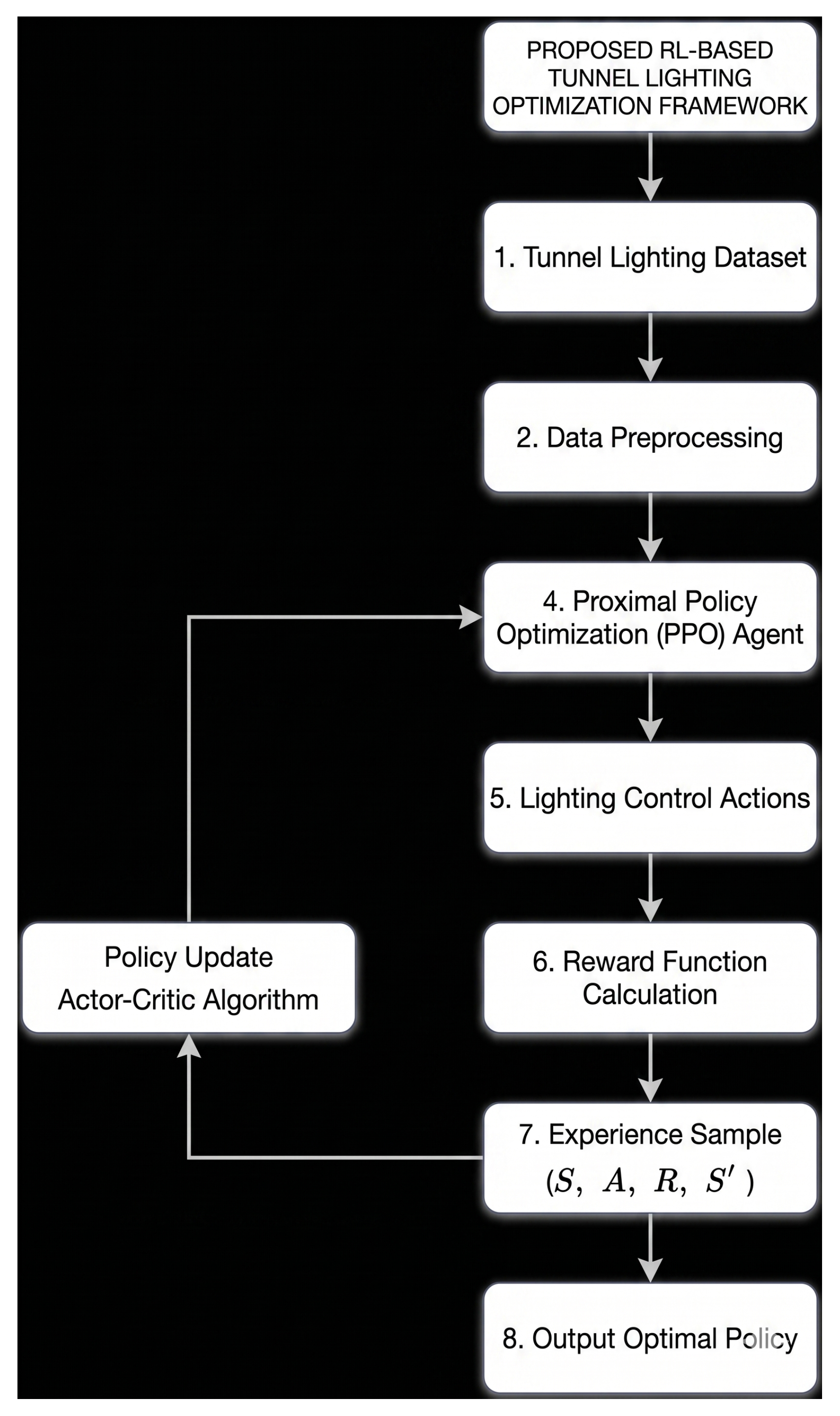
The dynamic dimming strategy of tunnel lighting based on PPO is presented in the figure. Firstly, the original operating data are collected from the tunnel lighting dataset and preprocessed through outlier elimination, data normalization and time series reconstruction to guarantee data reliability. On this basis, the state space is established with multidimensional environmental features, including traffic density, vehicle speed, ambient luminance and tunnel geographic location.Then, the PPO agent generates dimming actions through the policy network according to the current state, realizing dynamic brightness regulation of each lighting segment. After receiving the action, the environment computes the reward function that synthetically considers lighting performance, energy consumption and system stability, and produces state transition samples of .In this framework, the Actor–Critic structure is adopted to synchronously update the policy network and value network. The advantage function is employed to evaluate action quality, and the policy parameters are optimized by the clipped objective function of PPO. The whole workflow forms a closed-loop iterative mechanism of state perception–action decision-making–environmental feedback–policy updating, which finally achieves adaptive dynamic dimming control of tunnel lighting systems under complex operating conditions.
Figure 6.
Flowchart of the PPO-based dynamic dimming model for tunnel lighting.
3. Results
3.1. Experiments and Results Analysis
3.1.1. Data Sources and Experimental Parameter Settings
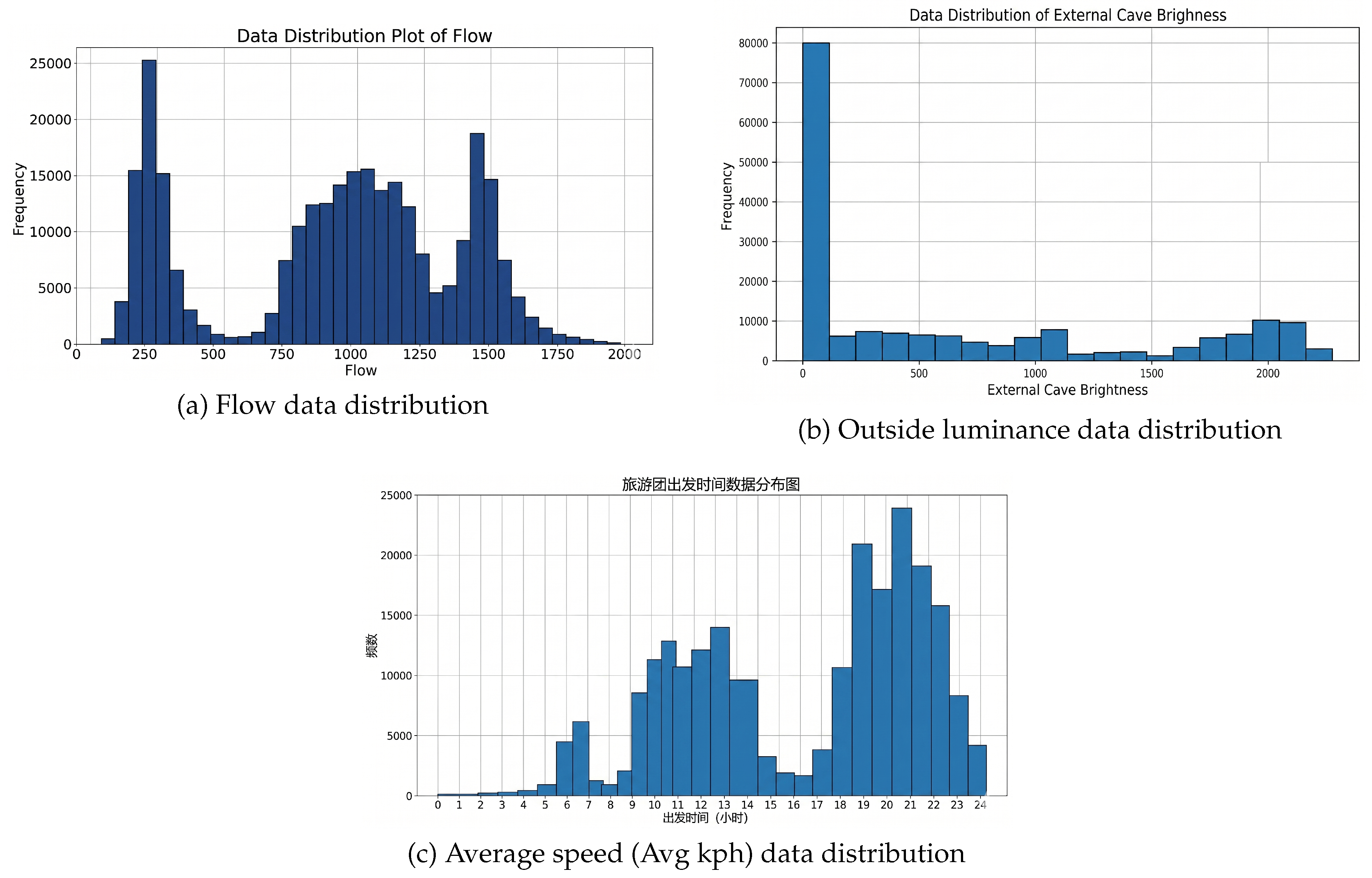
To verify the effectiveness of the PPO-based dynamic dimming strategy for tunnel lighting, an experimental environment is established using real-world operation data from the Shizuizi Tunnel in Jilin Province, where the proposed model is trained and tested. By organizing and modeling tunnel lighting scenario data, environmental states, dimming actions, and reward evaluation are integrated into a unified reinforcement learning framework. This allows the agent to iteratively optimize the control strategy in a data-driven manner, thereby achieving collaborative optimization of lighting quality and energy efficiency.
Figure 7.
Data Distribution Charts.
3.1.2. Model Training
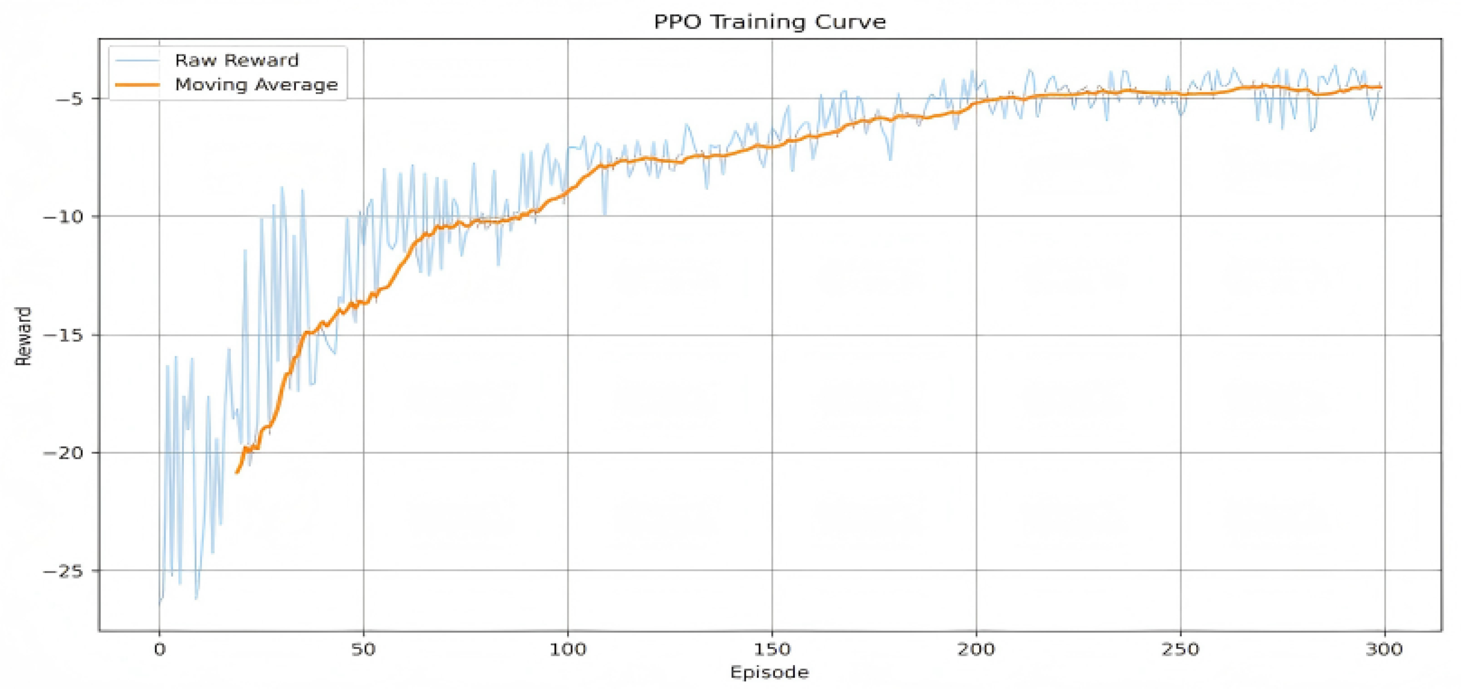
During model implementation, this paper constructs a dynamic dimming decision-making model for tunnel lighting based on the Proximal Policy Optimization (PPO) algorithm. At each time step, the agent generates corresponding dimming actions based on the current environmental state and applies them to the tunnel lighting system; the environment calculates a reward value based on the dimming results and performs a state transition, thereby forming experience samples for reinforcement learning training. During the training phase, the reward function comprehensively considers lighting effectiveness, visual comfort, system stability, and energy consumption levels, guiding the model to optimize its policy under multi-objective constraints. The model introduces a dominance function to evaluate the relative merits of actions, updates the policy network using the clipped objective function of the PPO algorithm, and estimates state values using the value network, thereby gradually improving the performance of the policy.
The entire training process follows an iterative mechanism of “sample collection—advantage estimation—policy update—value update.” In the early training stage, the model has not yet converged, and the actions generated by the agent exhibit significant randomness, leading to pronounced fluctuations in reward values. As training progresses, the model gradually learns the mapping between environmental states and dimming decisions; accordingly, the reward values show an overall upward trend and eventually stabilize.
The above training process demonstrates that the PPO algorithm can achieve continuous policy optimization under a stable update mechanism, gradually forming a control strategy that adapts to the dynamic dimming requirements of tunnel lighting.
3.1.3. Experimental Results and Analysis
To verify the control effectiveness of the PPO-based dynamic tunnel lighting dimming strategy under actual operating conditions, this paper compares and analyzes the operational results of the PPO strategy and the traditional L20 control strategy under typical diurnal variation conditions. The experimental results are primarily examined from four aspects: the zone-based brightness adjustment process, control characteristics in the entrance section, time-of-day energy-saving effects, and the spatial distribution of brightness across zones.
(1) Analysis of Zone Brightness Variation Results
As shown in Figure 8, this figure illustrates the variation of brightness in each functional zone of the tunnel over time under the traditional L20 control strategy. It can be observed that the brightness in the entrance section remains consistently higher than that in the other zones, with a significant increase during daytime hours, reaching its daily peak around noon. The brightness trends in the transition section, interior section, and exit section are largely consistent with those of the entrance section, exhibiting strong overall synchrony.This indicates that the L20 strategy primarily relies on external ambient brightness for zone compensation; when external brightness increases, the brightness of all zones is raised uniformly. While this method meets basic lighting requirements, its ability to differentiate adjustments between zones is limited. This can easily cause the high-brightness demand of the entrance section to spread to adjacent sections, thereby increasing the total lighting power of the entire tunnel.
Figure 8.
Reward Variation Curve During PPO Training.
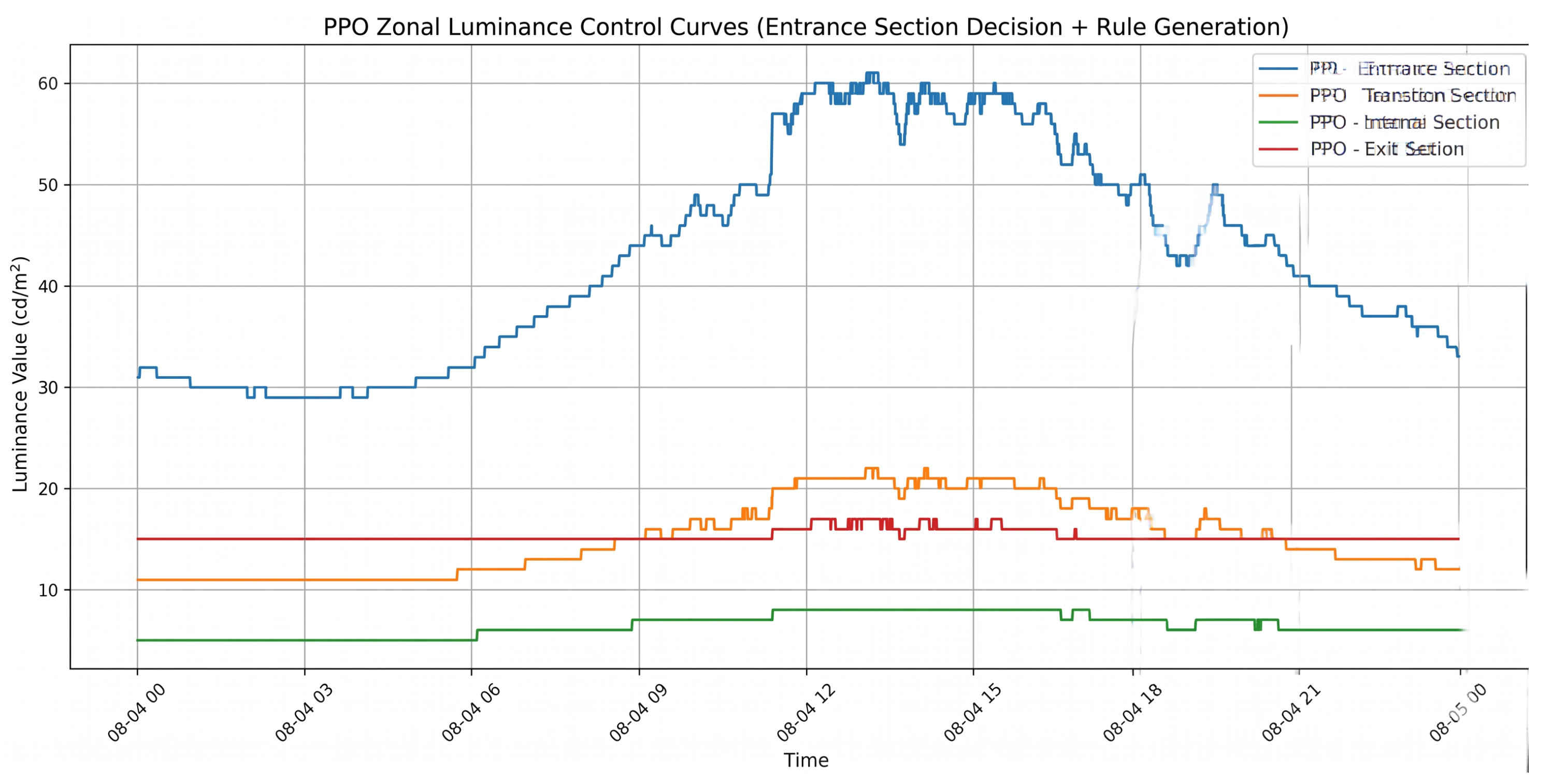
As shown in Figure 9, this figure illustrates the brightness variations across zones under the PPO dynamic dimming strategy.Compared to the traditional L20 method, the brightness curves for each zone under the PPO strategy are smoother. Although the entrance section still maintains the highest brightness, the peak value is significantly reduced, and the duration of high brightness is also shortened. The transition and interior sections do not exhibit a synchronous, substantial increase in brightness with the entrance section, and the brightness in the exit section changes relatively little overall, resulting in a more stable curve.These results indicate that the PPO strategy does not simply rely on direct mapping based on external brightness, but rather adaptively adjusts the lighting output of different zones through the joint optimization of environmental conditions, traffic conditions, and control benefits. The distribution of zone brightness is more refined, retaining the necessary high-brightness compensation capability for the entrance section while avoiding redundant lighting in non-critical sections.
Figure 9.
L20 Zone Luminance Control Curves.
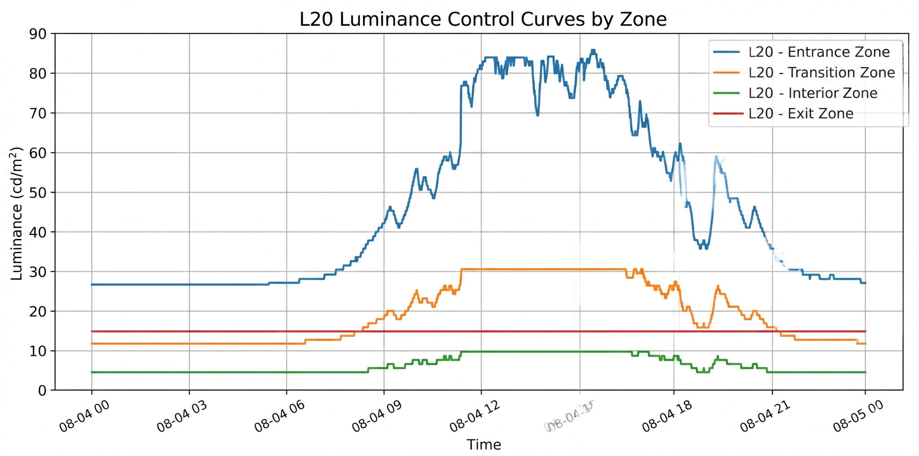
A comparison of the two figures reveals that the traditional L20 strategy tends to adopt a rule-driven, conservative control approach, with brightness settings typically set too high; the PPO strategy, however, exhibits more pronounced dynamic optimization characteristics, reducing unnecessary brightness output while meeting the functional requirements of each zone. These results demonstrate that reinforcement learning methods can effectively enhance the flexibility and rationality of zone dimming.
(2) Analysis of Brightness Control Results for the Entrance Section
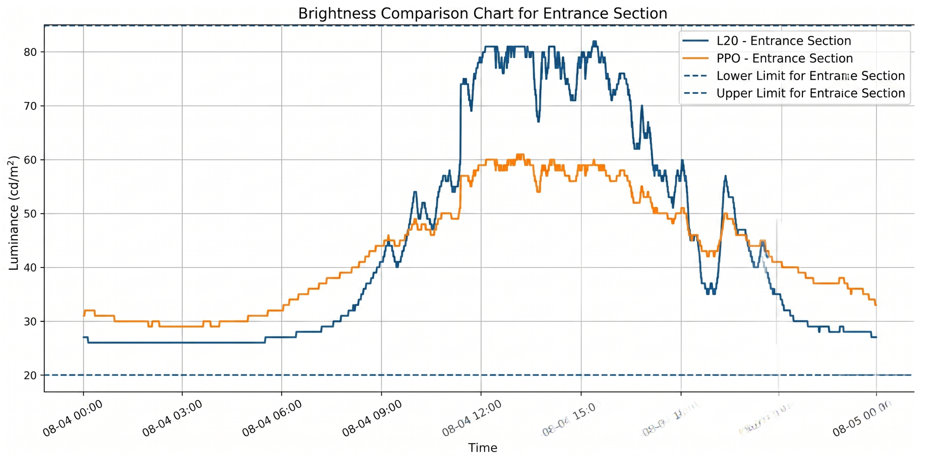
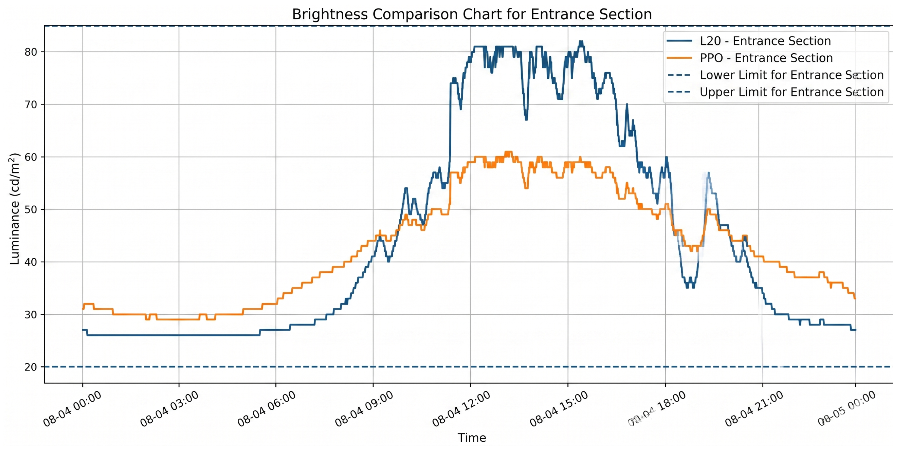
As shown in Figure 10, the L20 strategy and the PPO strategy exhibit significant differences in brightness control for the entrance section. Under the L20 strategy, brightness in the entrance section rises rapidly during high-brightness daytime periods and remains at a high level from noon through the afternoon, with peaks approaching the upper limit of the brightness constraint. This indicates that traditional methods typically reserve a large safety margin in entrance section control, which meets drivers’ visual adaptation needs but also tends to result in excessively high brightness output and increased energy consumption.
Figure 10.
Brightness Control Curves for Each Zone under the PPO Strategy.
Under the PPO strategy, the brightness in the entrance section can also be dynamically adjusted in response to changes in ambient brightness, but the overall variation is smoother, the peak control is more reasonable, and it remains within the constraint range at all times. Particularly during the high-brightness period at noon, the brightness in the entrance section under the PPO strategy is significantly lower than that under the L20 strategy, indicating that this method can effectively reduce redundant lighting while ensuring lighting safety, thereby improving the economic efficiency of the control.
Furthermore, during certain low-light periods in the early morning and at night, the entrance section brightness under the PPO strategy is slightly higher than that under the L20 strategy. This indicates that PPO does not simply pursue the lowest energy consumption but appropriately retains a certain margin of illumination under low-light conditions to improve visual comfort and driving safety. Overall, the PPO strategy achieves a good balance between safety and energy efficiency in entrance section control.
(3) Heatmap Analysis of the Traditional L20 Strategy
As shown in Figure 11, the temporal–spatial distribution of brightness in each tunnel zone under the conventional L20 control strategy is illustrated. A continuous and extensive high-brightness region appears in the entrance section from noon to afternoon, indicating a long period of high-intensity lighting output. Meanwhile, the transition and interior sections also show a significant brightness increase during the same period, implying that the high-brightness demand of the entrance section strongly affects adjacent zones.
Figure 11.
Comparison of Entrance Brightness.
This heatmap pattern reveals that the L20 strategy follows a typical characteristic of “high brightness in the entrance section driving global brightness elevation” under strong ambient light conditions. Although this design helps quickly establish sufficient lighting safety margins, it also passively increases the brightness of non-critical sections and reduces the independence of zoning control. From an energy-saving perspective, such a distribution significantly increases the overall power consumption of the tunnel system, which is the main reason for the limited energy efficiency of traditional rule-based control methods.
(4) PPO Strategy Heat Map Analysis As shown in Figure 12, this figure depicts the brightness heat distribution across zones under the PPO dynamic dimming strategy. Compared to the L20 heatmap, the entrance section remains the brightest area under the PPO strategy, but the coverage of the high-brightness zone is significantly reduced, and its duration is markedly shorter. The brightness distribution in the transition and interior sections is more balanced, with no widespread synchronous increase following the entrance section, while the brightness in the exit section remains relatively stable.
Figure 12.
L20 Zone-by-Zone and Time-of-Day Average Illuminance Heat Map.
These results indicate that the PPO strategy more accurately identifies the lighting requirements of different functional sections. The entrance section retains the necessary high-brightness compensation capability to meet the driver’s visual adaptation needs; meanwhile, the transition and interior sections are regulated more independently based on their own states, avoiding the problem of excessive spatial propagation of brightness demands found in traditional methods. The contraction of high-value areas in the heatmap directly demonstrates that the PPO strategy reduces redundant lighting output and improves the utilization efficiency of brightness resources.
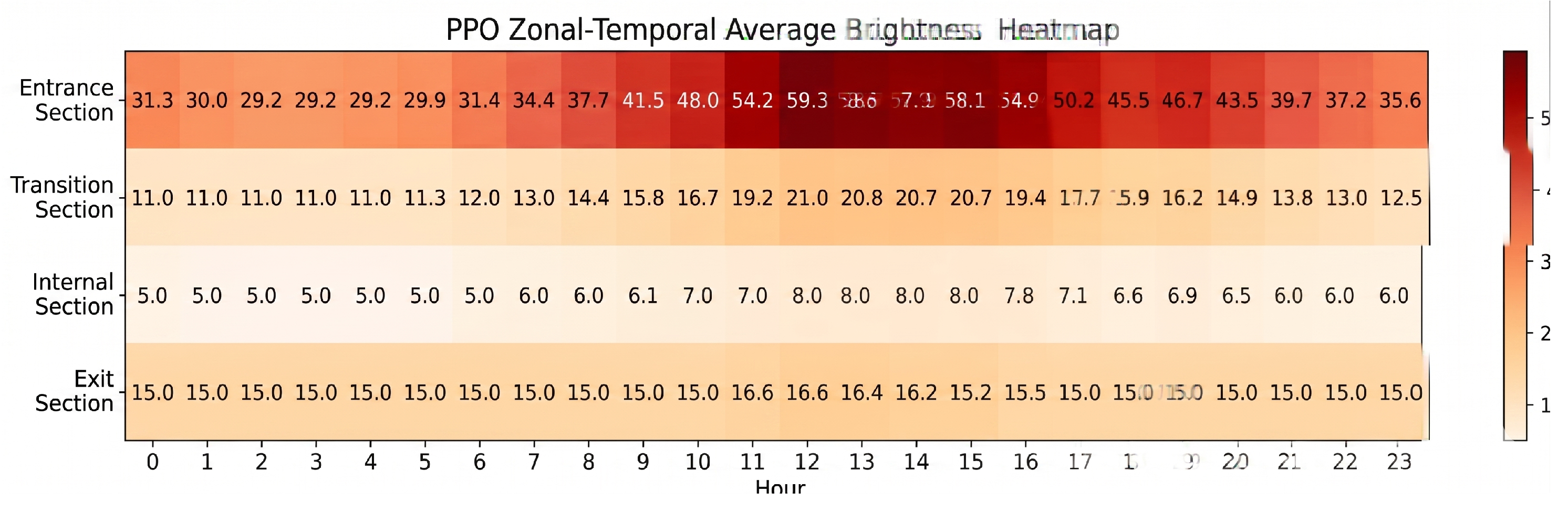
Further analysis of the energy-saving rate curves reveals that the fundamental reason for the PPO strategy’s superior energy-saving performance during daytime high-brightness periods lies in the effective control of high-brightness areas in its heatmap. In other words, energy savings do not stem from simply reducing brightness in a single zone, but rather from the overall optimization of the brightness structure across all zones.
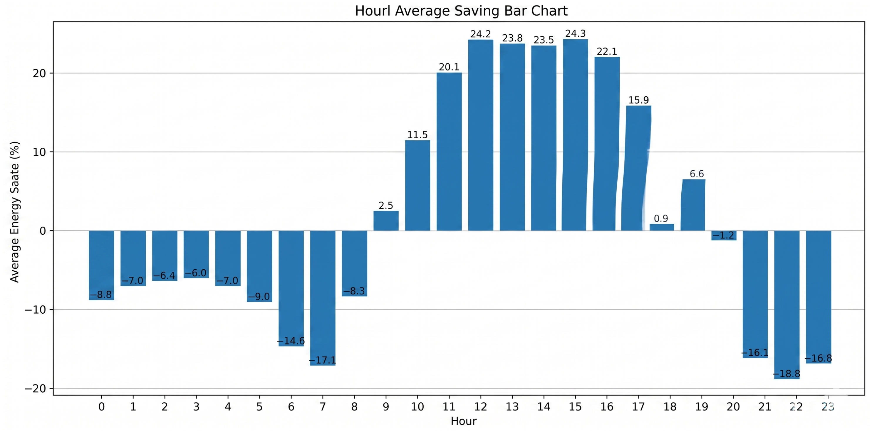
As shown in Figure 13, the energy-saving rate of the PPO strategy relative to the conventional L20 strategy varies considerably across different time intervals, indicating distinct control performances of the two methods under diverse operating conditions.
Figure 13.
PPO Zone-by-Zone and Time-of-Day Average Brightness Heatmap.
During 10:00–17:00, the PPO strategy achieves outstanding energy-saving efficacy, especially from 11:00 to 16:00, when the energy-saving rate stays above 20% at most moments and reaches a peak of nearly 24%. This result reveals that the conventional L20 strategy presents obvious over-illumination under high external brightness during the daytime. In contrast, the PPO strategy effectively reduces the total energy consumption of the system by suppressing excessive brightness in the entrance section and restraining synchronous brightness uplift in adjacent zones, showing stronger adaptive optimization ability.
After 18:00, the energy-saving rate declines gradually, with only slight energy savings in certain periods. This phenomenon implies that the tunnel lighting system operates at a low-power level with the decrease in external brightness, leaving limited optimization space; thus, the gap in energy consumption between the two strategies is narrowed.
During specific early-morning and nighttime periods, the energy-saving rate becomes negative, meaning that the energy consumption of the PPO strategy is slightly higher than that of the L20 strategy. Combined with the brightness variation of the entrance section, this is mainly because the PPO strategy properly raises the brightness of partial sections under low-illuminance conditions. Although the energy consumption increases marginally in these periods, the lighting continuity and visual safety margin are both improved. This confirms that the PPO strategy does not take energy saving as the only goal, but balances energy efficiency and lighting safety comprehensively, giving priority to safety when the two objectives conflict.
Figure 14.
Bar Chart of Time-of-Day Average Energy Savings.
4. Discussion
The proposed PPO-based tunnel lighting dimming strategy solves the problems of poor adaptability and low energy efficiency of the traditional L20 method. It exhibits better performance in dimming smoothness, zoning control and energy conservation. This strategy achieves significant energy savings in the daytime while prioritizing driving safety. This study is only verified with data from a single tunnel, so the model generalization needs to be improved. In future work, we will expand the dataset and combine IoT technology to promote its engineering application.
5. Conclusions
This paper addresses the issues of limited adaptability and energy efficiency optimization in traditional tunnel lighting control methods by proposing a dynamic dimming strategy based on the PPO algorithm. By constructing a multidimensional state space, a continuous action space, and a multi-objective reward function, the strategy achieves the coordinated optimization of lighting safety and energy consumption.Experimental results demonstrate that the proposed method enables refined, zone-based control based on traffic conditions and ambient illumination, effectively reducing redundant lighting while ensuring lighting safety. Compared to the traditional L20 strategy, this method achieves better energy-saving performance during high-illumination periods and simultaneously meets visual safety requirements under low-illumination conditions. In summary, the proposed PPO dimming strategy exhibits excellent performance in terms of adaptability and energy efficiency, providing a valuable reference for intelligent tunnel lighting control.
6. Patents
No patents were generated from the work reported in this manuscript.
Author Contributions
Conceptualization, J.H. and Z.C.; methodology, J.H.; software, J.H.; validation, J.H., Z.B. and B.L.; formal analysis, J.H.; investigation, J.H.; resources, Z.C.; data curation, J.H. and Z.B.; writing—original draft preparation, J.H.; writing—review and editing, Z.C. and Z.B.; visualization, J.H.; supervision, Z.C.; project administration, Z.C. All authors have read and agreed to the published version of the manuscript.
Funding
This research received no external funding.
Institutional Review Board Statement
Not applicable.
Informed Consent Statement
Not applicable.
Data Availability Statement
The data presented in this study are available on request from the corresponding author.
Acknowledgments
The authors acknowledge the data support from the Shizuizi Tunnel in Jilin Province.
Conflicts of Interest
The authors declare no conflicts of interest.
References
- Du, G. Design of Tunnel Lighting Control System Based on Fuzzy PID. Master’s Thesis, Hangzhou Dianzi University, Hangzhou, China, 2020. [Google Scholar] [CrossRef]
- Miao, S. Research on Intelligent Dimming Control Technology of Expressway Tunnel Lighting. Master’s Thesis, University of Chinese Academy of Sciences, Beijing, China, 2020. [Google Scholar] [CrossRef]
- Hu, K.; Li, J.; Zhou, B. Construction of On-Demand Dimming Model for Tunnel Lighting Based on Deep Reinforcement Learning. Informatiz. Res. 2025, 51, 140–143. [Google Scholar]
- Yong, P.; Pan, Y.; Wang, F. Research and Application of Dimming Control System for Highway Tunnel Lighting on Demand. IOP Conf. Ser. Earth Environ. Sci. 2020, 587, 012083. [Google Scholar] [CrossRef]
- R, X.; H, Y.; B, H. Intelligent Dimming Control and Energy Consumption Monitoring System of Tunnel Lighting. Light. Res. Technol. 2024, 56, 72–86. [Google Scholar] [CrossRef]
- Suying, L.; Chenfei, J.; Chong, Z. Tunnel Lighting Intelligent Control System Based on Ambient Light Ratio. J. Phys. Conf. Ser. 2021, 1865, 022019. [Google Scholar] [CrossRef]
- Liu, S.; Chen, R.; Xu, C. Towards a Human-Centric Intelligent Lighting System in Expressway Tunnels: A Deep Learning Based Framework for Luminance Demand Prediction. Hum.-Centric Intell. Syst. 2026, 6, 1. [Google Scholar] [CrossRef]

Table 1.
Illuminance Reduction Coefficients for the Entrance Section k.
| Design Hourly Traffic Volume | Design Speed (km/h) | |||||
|---|---|---|---|---|---|---|
| One-way Traffic | Two-way Traffic | 120 | 100 | 80 | 60 | 20–40 |
| 0.070 | 0.045 | 0.035 | 0.022 | 0.012 | ||
| 0.050 | 0.035 | 0.025 | 0.015 | 0.010 | ||
Table 2.
Intermediate Section Illuminance Table.
| Design Speed (km/h) | Lin | |||||
| One-Way Traffic | Two-Way Traffic | |||||
| (veh/(h·ln)) | (veh/(h·ln)) | |||||
| 120 | 10.0 | 6.0 | 4.5 | 10.0 | 6.0 | 4.5 |
| 100 | 6.5 | 4.5 | 3.0 | 6.5 | 4.5 | 3.0 |
| 80 | 3.5 | 2.5 | 1.5 | 3.5 | 2.5 | 1.5 |
| 60 | 2.0 | 1.5 | 1.0 | 2.0 | 1.5 | 1.0 |
| 20–40 | 1.0 | 1.0 | 1.0 | 1.0 | 1.0 | 1.0 |
Disclaimer/Publisher’s Note: The statements, opinions and data contained in all publications are solely those of the individual author(s) and contributor(s) and not of MDPI and/or the editor(s). MDPI and/or the editor(s) disclaim responsibility for any injury to people or property resulting from any ideas, methods, instructions or products referred to in the content. |
© 2026 by the authors. Licensee MDPI, Basel, Switzerland. This article is an open access article distributed under the terms and conditions of the Creative Commons Attribution (CC BY) license.
Copyright: This open access article is published under a Creative Commons CC BY 4.0 license, which permit the free download, distribution, and reuse, provided that the author and preprint are cited in any reuse.