
Submitted:
09 May 2026
Posted:
11 May 2026
You are already at the latest version
Abstract
To address the complex spatiotemporal dependencies and dynamically evolving spatial relationships in tunnel traffic flow prediction, a macro–micro collaborative two-stage prediction method is proposed.The Grey Wolf Optimizer (GWO) is first employed to optimize the GRU model for predicting incoming traffic flow at the tunnel entrance, providing reliable macro-level input for subsequent modeling.Based on this, a spatiotemporal graph structure is constructed, and an FSE-ST-GCN model integrating an adaptive adjacency matrix with spatial and channel attention mechanisms is developed to capture dynamic spatial dependencies and enhance key feature representation.Experiments are conducted using real-world traffic flow data collected from the Shizuizi Tunnel on the Jilin–Caoshi Expressway. The results show that the proposed method outperforms baseline models in terms of MAE, RMSE, and MAPE, achieving superior prediction accuracy and stability. This work provides effective technical support for refined tunnel traffic management and lighting control.
Keywords:
tunnel traffic flow prediction
; ST-GCN
; adaptive adjacency matrix
; spatial attention
; channel attention
1. Introduction
Traffic flow prediction is a crucial component of intelligent transportation systems. Given its complex spatio-temporal characteristics, scholars both domestically and internationally have conducted extensive research in this area. Early studies predominantly employed traditional time series methods, such as the ARIMA model, to achieve short-term predictions through analysis of the stationarity of traffic flow data. While effective in small-scale data scenarios, these methods struggle to capture the nonlinear and complex dynamic characteristics of traffic flow.
With the advancement of deep learning, neural network-based methods have gradually become the mainstream. Duan Zhongxing et al. [1]predicted tunnel traffic flow using an LSTM model combined with the Grey Wolf optimization algorithm, effectively improving prediction accuracy; Chen Jiahang et al. [2]proposed the CGO-CNN model, which combines optimization algorithms with convolutional neural networks to enhance short-term traffic flow prediction performance; Sun Zhijuan et al. [3]utilized YOLOv8 and object tracking algorithms to perform traffic flow detection and statistics, providing high-quality data support for prediction models. However, such methods often focus on modeling temporal features and lack the ability to adequately capture spatial dependencies.
To enhance spatial modeling capabilities, graph convolutional networks (GCNs) have been widely applied in traffic flow prediction. Zhang et al. [4] proposed a spatio-temporal graph convolutional network based on attention mechanisms, which effectively improved prediction accuracy by introducing an adaptive adjacency matrix to learn dynamic spatial relationships. Su et al. [5]further integrated spatial and frequency-domain attention mechanisms to enable multidimensional feature modeling, thereby improving the model’s adaptability to complex traffic patterns. However, methods relying on fixed graph structures or single attention mechanisms still struggle to comprehensively capture the dynamic spatial dependencies of traffic flow.
In recent years, multi-structure and multi-scale fusion methods have gradually become a research hotspot. Yuan et al. [6]proposed the GDLP-Net model, which uses a dual-branch structure to model global dynamic features and local propagation features separately, thereby achieving multi-scale information fusion; Zhang et al. [7]proposed the FGT-Net model, which enhances the stability and interpretability of traffic flow prediction through a multi-granularity fuzzy fusion mechanism; Ye et al[8].proposed the Dual Graph Fusion Network (STDGFN), which uses a multi-graph structure to mitigate the oversmoothing issue in graph convolutions and enhance the expression of spatial features. These methods demonstrate stronger modeling capabilities in complex traffic scenarios.
Although existing research has made significant progress in traffic flow prediction, certain limitations remain: first, there is a lack of a unified fusion mechanism for multi-source spatial relationships; second, attention mechanisms are often confined to a single dimension, making it difficult to simultaneously account for both spatial and lane-level features; third, in complex traffic scenarios, the models’ ability to capture dynamic spatial dependencies and key features still has room for improvement.Based on this, this paper builds upon the ST-GCN model by integrating an adaptive adjacency matrix, spatial attention mechanisms, and lane-level attention mechanisms to construct the FSE-ST-GCN model. This approach achieves the fusion of multi-source spatial relationships and the enhancement of multi-dimensional features, thereby improving traffic flow prediction accuracy and model stability.
Although existing studies have made significant progress in traffic flow prediction, several limitations remain. First, there is a lack of a unified and effective mechanism for fusing multi-source spatial relationships. Second, most existing attention mechanisms focus on a single dimension, making it difficult to jointly model spatial and channel features. Third, in complex traffic scenarios, the capability of models to capture dynamic spatial dependencies and critical features remains insufficient.
To address these issues, this paper proposes a macro–micro collaborative two-stage traffic flow prediction framework. In the first stage, the Grey Wolf Optimizer (GWO) is employed to optimize the key hyperparameters of the Gated Recurrent Unit (GRU) model, enabling accurate prediction of traffic flow at the tunnel entrance and providing reliable macro-level inputs for subsequent modeling. In the second stage, based on the macro-level predictions, a graph representation of multiple monitoring points inside the tunnel is constructed, and an FSE-ST-GCN model integrating adaptive adjacency matrix, spatial attention, and channel attention mechanisms is developed. The model realizes dynamic fusion of multi-source spatial relationships and strengthened feature representation, thereby supporting fine-grained, distributed prediction of traffic flow over different tunnel segments.
Overall, the proposed method not only improves prediction accuracy but also enhances the model’s ability to capture complex spatiotemporal dependencies and maintain stability, providing effective support for refined tunnel traffic state perception and related applications.
2. Materials and Methods
2.1. Macro Traffic Flow Prediction Method Based on GWO-GRU
Refined regulation of tunnel lighting systems hinges on the prospective prediction of traffic flow states. However, conventional approaches struggle to balance macro traffic inputs and the internal evolutionary process of the tunnel, rendering their prediction results inadequate for meeting the control requirements of on-demand, zonal, and gradual adjustment. To address this limitation, this study introduces the Grey Wolf Optimizer (GWO) to perform global optimization on the key hyperparameters of the Gated Recurrent Unit (GRU) model, including the number of hidden layer neurons, time steps, learning rate, dropout rate, and batch size. A GWO-GRU model for predicting arriving traffic flow at the tunnel is thereby constructed. This method effectively mitigates the reliance of parameter selection on manual experience, avoids trapping in local optima, and consequently enhances the accuracy and robustness of traffic flow prediction.
2.1.1. Optimization Methodology of the GWO-GRU Model
This study first employs GWO to optimize the critical hyperparameters of the GRU model. By simulating the cooperative behaviors exhibited by grey wolf packs during hunting, the GWO algorithm conducts global search within the hyperparameter space, which effectively overcomes the drawback that traditional hyperparameter selection methods are prone to falling into local optima.Five key hyperparameters are optimized in this research: the number of hidden layer neurons, time steps, learning rate, dropout rate, and batch size. The optimized hyperparameter configurations are presented as follows:

Table 1.
Hyperparameter Optimization Results.
| Number of hidden layer neurons | Time steps | Learning rate | Dropout rate | Batch size |
|---|---|---|---|---|
| 85 | 39 | 0.000941 | 0.186825 | 58 |
The GWO algorithm is adopted to conduct hyperparameter optimization for the GRU model, which effectively avoids the limitations of traditional manual parameter tuning and significantly improves the training stability and prediction accuracy of the model.In the model training phase, the number of iterations is set to 100 epochs, and the batch size is set to 58. The Adam optimizer and mean squared error (MSE) loss function are adopted. The iterative updating of model parameters is completed based on the training and validation datasets.
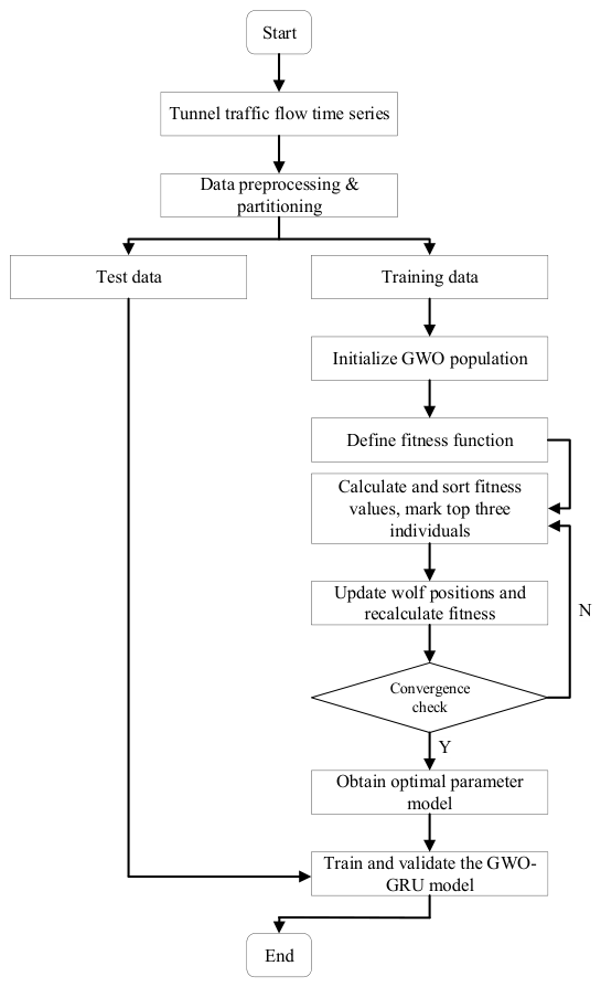
Figure 1.
Training Flow of the GWO-GRU Model.
2.1.2. Model Performance Comparison and Validation
To verify the effectiveness of the GWO-GRU model in predicting arriving traffic flow at the tunnel, comparative experiments are conducted against the conventional GRU model with manually tuned hyperparameters under the same dataset and evaluation metrics. Mean Squared Error (MSE), Root Mean Squared Error (RMSE), and Mean Absolute Percentage Error (MAPE) are adopted as evaluation indicators. Experimental results show that the GWO-GRU model achieves faster convergence and lower loss values, demonstrating superior training efficiency and stability.
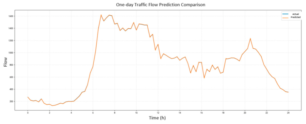
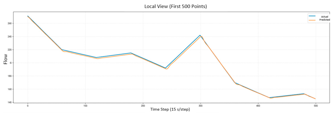
Figure 2.
Comparison of Tunnel Arrival Traffic Flow Prediction.
Figure 3.
Local Enlarged View of Tunnel Arrival Traffic Flow Prediction.
In contrast, the conventional GRU model converges more slowly and yields higher final prediction errors. The results demonstrate that GWO optimization can effectively enhance the global optimization capability of the model, thereby improving the overall prediction performance.
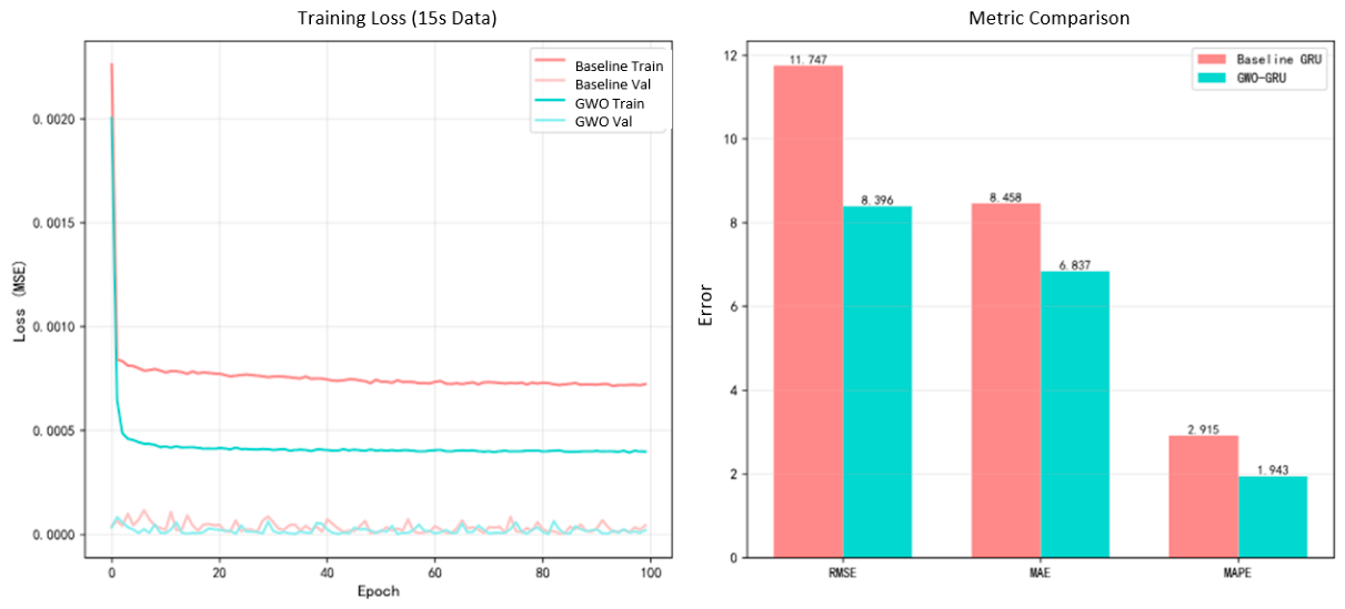
Figure 4.
Training Comparison between GWO-GRU and Conventional GRU.
In addition, the comparison results of MSE, RMSE and MAPE show that the GWO-GRU model outperforms the conventional GRU model across all evaluation metrics. The MSE and RMSE are reduced remarkably, and the MAPE also achieves a lower relative error, which verifies that the proposed model possesses higher prediction accuracy and stability.
Table 2.
Error Comparison between GWO-GRU and Conventional GRU.
| Model | MSE | RMSE | MAPE |
|---|---|---|---|
| Conventional GRU | 8.458 | 11.747 | 2.915 |
| GWO-GRU | 6.837 | 8.396 | 1.943 |
From the prediction comparison curves, it can be observed that the predicted values of the GWO-GRU model achieve a higher fitting degree with the actual values. The model maintains a small prediction error over a long time span and presents a smoother curve trend. In contrast, the conventional GRU model deviates obviously from the real observations, and its prediction error gradually increases over time. This indicates that the conventional GRU exhibits poor stability in long-term time series prediction and cannot accurately capture the variation trend of traffic data.
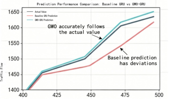
Figure 5.
Prediction Comparison between GWO-GRU and Conventional GRU.
2.2. Microscopic Spatiotemporal Prediction of Traffic Flow Based on FSE-ST-GCN
Tunnel traffic flow exhibits strong spatiotemporal correlations. To effectively capture its spatial distribution and temporal evolution patterns, it is modeled as a spatiotemporal graph. Considering the discrepancies in traffic conditions across different tunnel segments, each monitoring section is represented as a graph node to construct the spatial topology, thereby accurately characterizing the spatial heterogeneity of tunnel traffic flow.
At the input layer, the GWO-GRU model is employed to predict incoming traffic flow at the tunnel entrance, providing stable macro-level information support for the FSE-ST-GCN model. This information, combined with real-time observed data from each tunnel segment, constitutes the input features of the spatiotemporal graph.
The FSE-ST-GCN model integrates Graph Convolutional Networks (GCN) with spatiotemporal attention mechanisms. Specifically, spatial dependencies among nodes and temporal dynamics are separately captured through spatial attention and temporal attention modules, enabling joint spatiotemporal modeling and effective feature extraction for tunnel traffic flow prediction.
2.2.1. Spatio-Temporal Graph Modeling of Tunnel Traffic Flow
(1) Segmentation Node Modeling
The tunnel is partitioned into four segments: entrance, transition, middle, and exit segments. Each segment is modeled as a graph node, representing the traffic flow state of the corresponding segment at a specific time step. Let denote the traffic flow of the i-th tunnel segment at time t. Accordingly, the overall traffic state of the tunnel at time t can be formulated as follows:
This modeling paradigm transforms tunnel traffic flow from a one-dimensional time series into graph-structured node representations, providing a solid foundation for subsequent graph neural network modeling.
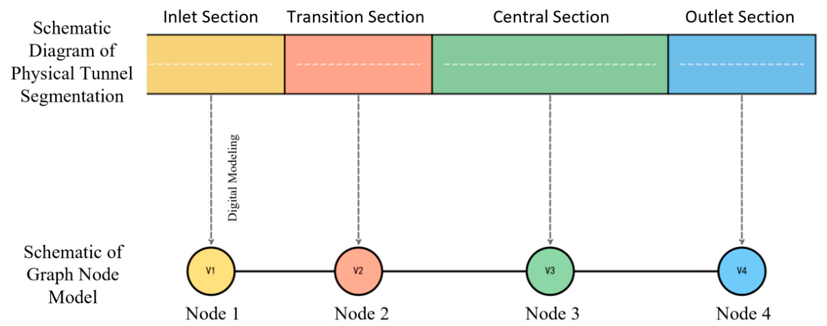
Figure 6.
Schematic diagram of tunnel segments and nodes.
(2) Spatial Topological Modeling
To characterize spatial dependencies across tunnel segments, the tunnel traffic system is formulated as a graph , where the adjacency matrix A encodes the connection relationships between graph nodes. In accordance with the physical structure of the tunnel, only adjacent inter-segment connections are considered, and self-loops are incorporated to derive:
where denotes the identity matrix. This adjacency topology captures the propagation pathways of traffic flow within the tunnel, laying a solid foundation for subsequent graph convolution operations.
The spatial topology of the tunnel is illustrated below:
2.2.2. Adaptive Adjacency Matrix
(1) Construction of the Adaptive Adjacency Matrix
Let N denote the total number of segment nodes within the tunnel. For each node, two embedding matrices are learned:
where and represent the source and target embeddings of graph nodes, respectively, and d denotes the dimension of embedding space. By calculating the similarity between node embedding vectors, inter-node correlation relationships are derived to construct the correlation matrix:
Subsequently, normalization is conducted via the Softmax function to obtain the adaptive adjacency matrix:
Driven by raw traffic flow data, this matrix adaptively captures latent spatial dependencies across tunnel segments, thereby overcoming the inherent limitations of pre-defined fixed topological structures.
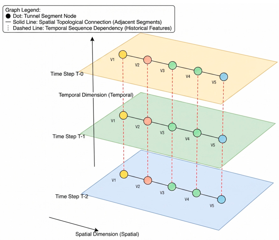
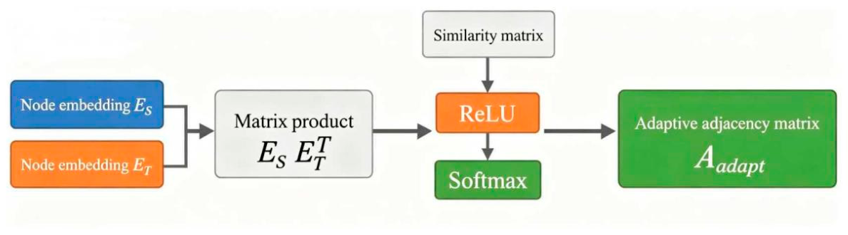
Figure 7.
Spatial Topology Diagram of Tunnel Segments.
Figure 8.
Schematic diagram of the adaptive adjacency matrix generation process.
(2) Fusion of Adjacency Matrix Modeling
To integrate the physical prior of tunnel topology with data-driven dynamic inter-segment dependencies, the static adjacency matrix is fused with the adaptive adjacency matrix to form a unified spatial representation:
wheredenotes the static physical adjacency matrix,represents the adaptive adjacency matrix, and is a learnable parameter that balances their contributions.
This fusion strategy preserves the inherent physical connectivity of tunnel segments while simultaneously capturing latent traffic propagation patterns, thereby improving the model’s capability in spatial feature representation.
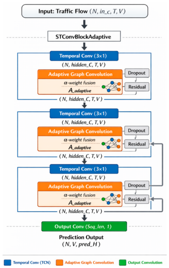
Figure 9.
Adaptive ST-GCN Model Architecture.
By introducing the adaptive adjacency matrix, the model is able to dynamically learn latent node relationships from data and integrate them with the original topological structure. This enhances its capability to capture complex spatial dependencies in traffic flow, providing a more flexible and effective representation for spatio-temporal graph convolutional modeling.
2.2.3. Channel Attention Mechanism
(1) Principle of the Channel Attention Mechanism
The channel attention mechanism models channel-wise statistics of feature maps to learn the importance of each feature channel. Input features are first aggregated using global average pooling and global max pooling to capture complementary channel-level representations. The two feature descriptors are then projected through a shared multi-layer perceptron (MLP) and fused. Channel attention weights are subsequently generated via a Sigmoid activation function, and applied to recalibrate the original feature maps through channel-wise weighting.
This mechanism adaptively emphasizes informative feature channels and suppresses less relevant responses, thereby enhancing feature discriminability.
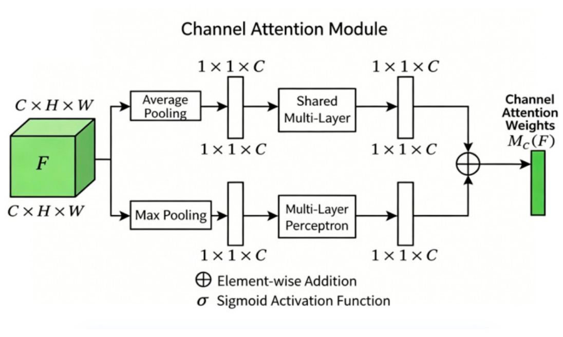
Figure 10.
Schematic diagram of the channel attention module.
(2) Implementation of the SE Module
For practical implementation, the Squeeze-and-Excitation (SE) block is adopted to construct the channel attention module. The architecture is divided into two core operations: Squeeze and Excitation.
Squeeze: Input feature maps are aggregated through global average pooling to produce holistic channel-wise statistical descriptors.
Excitation: A two-layer fully-connected network captures inter-channel nonlinear dependencies and adaptively generates corresponding channel attention weights.
Finally, the obtained weights are multiplied with the original feature maps in a channel-wise manner to amplify informative channels and suppress redundant ones.
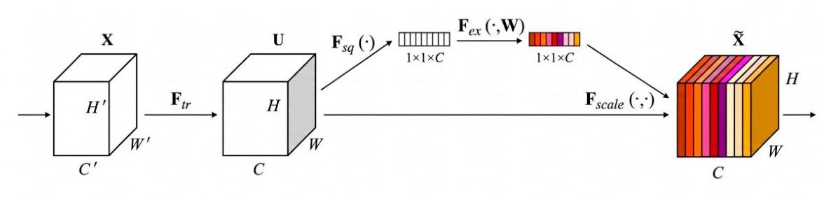
Figure 11.
SE block architecture diagram.
By embedding the SE channel attention module into the spatio-temporal convolutional module of ST-GCN, the importance of channel features can be modeled, thereby enhancing the model’s focus on key discriminative features. Based on these improvements, the SE-ST-GCN network architecture is developed.
In summary, the introduced channel attention mechanism enables the model to extract critical feature information more effectively and strengthen its representation capacity for spatio-temporal dependencies of traffic flow, thereby boosting overall prediction accuracy and stability.
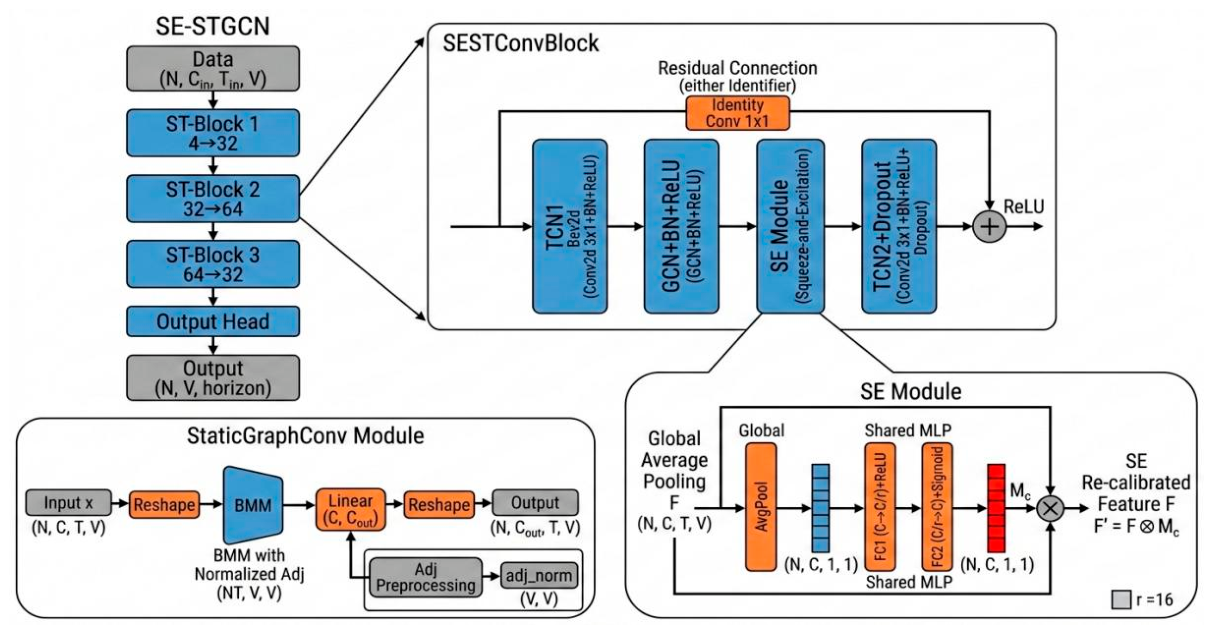
Figure 12.
SE-ST-GCN Model Architecture.
2.2.4. Spatial Attention Mechanism
(1) Principle of the Spatial Attention Mechanism
The core intuition of the spatial attention mechanism is to adaptively compute inter-node correlation weights according to node features, so as to quantify the mutual influence across tunnel segments. Specifically, node features are projected to measure inter-node correlations, yielding an attention weight matrix that encodes spatial dependencies. These weights are then normalized to achieve consistent comparability among inter-node influence scores.
By dynamically adjusting inter-node dependencies according to real-time traffic flow conditions, this mechanism enables the model to prioritize segments that dominate traffic flow propagation. As a result, the model’s capacity for spatial feature extraction is further improved.
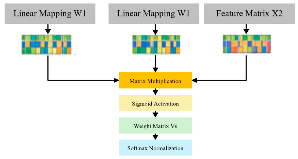
Figure 13.
Flowchart of the Spatial Attention Mechanism.
(2) Spatial Attention Modeling
Based on the aforementioned mechanism, spatial attention is employed to construct a spatial attention matrix that captures dynamic inter-node relationships. This matrix encodes the time-varying dependencies between tunnel segments as traffic conditions change, effectively addressing the inherent limitations of traditional fixed adjacency matrices.
Compared with modeling approaches that rely solely on physical topology, the spatial attention mechanism excavates latent spatial dependencies from traffic data, allowing the model to more flexibly and accurately depict the propagation patterns of traffic flow within tunnels.
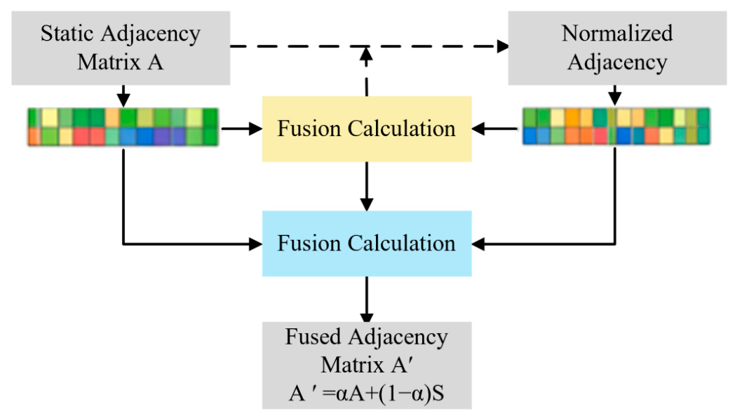
Figure 14.
Schematic of the Dynamic Adjacency Matrix Fusion Mechanism.
In summary, the introduction of the spatial attention mechanism enables adaptive weighting of the importance of different nodes, enhancing the model’s capability to capture key regions and their spatial dependencies. This further refines the modeling of spatial dependencies in tunnel traffic flow, while experimental results demonstrate that this mechanism effectively reduces prediction errors, improves model accuracy, and enhances the model’s stability and robustness.
2.2.5. Construction of the FSE-ST-GCN Model
(1) Overall Model Structure
The FSE-ST-GCN adopts a multi-layer spatio-temporal convolutional architecture, consisting of an input layer, multiple spatio-temporal convolutional modules (ST-Conv Blocks), and an output layer. The input consists of traffic flow sequences of each tunnel segment within a continuous time window, while the output generates traffic flow predictions for subsequent time steps.
In terms of network architecture, the model stacks multiple ST-Conv Blocks to extract temporal and spatial features of traffic flow layer by layer. During the feature extraction process, various enhancement mechanisms are integrated to effectively model complex spatio-temporal dependencies between traffic flow features.
(2) ST-Conv Block Structural Design
The ST-Conv Block is the core computational unit of the FSE-ST-GCN model. Its internal structure consists of a temporal convolution layer, a fusion graph convolution layer, another temporal convolution layer, and a residual connection. The specific process is as follows:
1. Temporal Convolution Layer: Extracts local dynamic changes in traffic flow along the temporal dimension;
2. Fusion Graph Convolution Layer: Models the spatial dependencies between tunnel segments;
3. Temporal Convolution and Dropout Layer: Further refines temporal features and suppresses overfitting;
4. Residual Connection: Preserves original information and enhances model training stability.
Through this architecture, the model can simultaneously learn the temporal evolution patterns and spatial propagation characteristics of traffic flow at each layer.
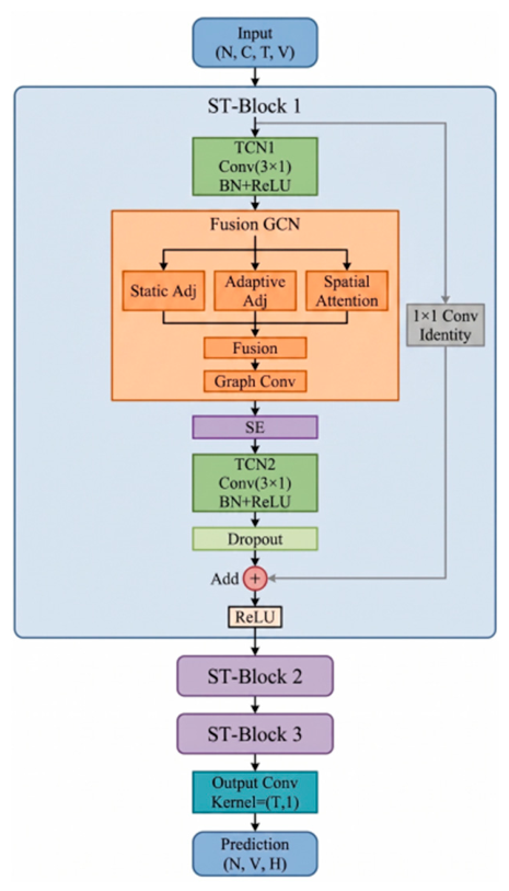
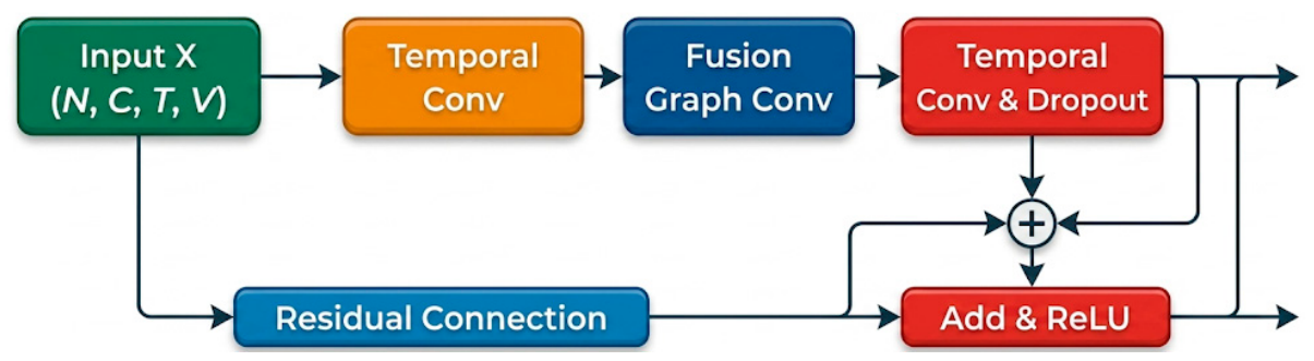
Figure 15.
Overall Architecture of the FSE-ST-GCN Network.
Figure 16.
Internal structure of the ST-Conv Block.
(3) Fusion Graph Convolution Mechanism
To enhance the model’s ability to capture complex spatial dependencies, this paper introduces a fused graph convolutional mechanism within the graph convolutional module to unify the modeling of various spatial relationships. Specifically, these include: static adjacency relationships, which describe the physical topological structure between tunnel segments; adaptive adjacency relationships, which learn latent spatial associations through a data-driven approach; and spatial attention relationships, which dynamically characterize the influence weights inter-node.
Based on the above three types of spatial relationships, a unified spatial dependency representation is constructed:
Here, represents the fixed adjacency matrix, represents the adaptive adjacency matrix, represents the spatial attention matrix, and represents the learnable weight parameters.
This fusion method can dynamically capture the implicit propagation paths and key spatial dependencies of traffic flow while preserving the tunnel topology, thereby significantly enhancing spatial feature representation capabilities.
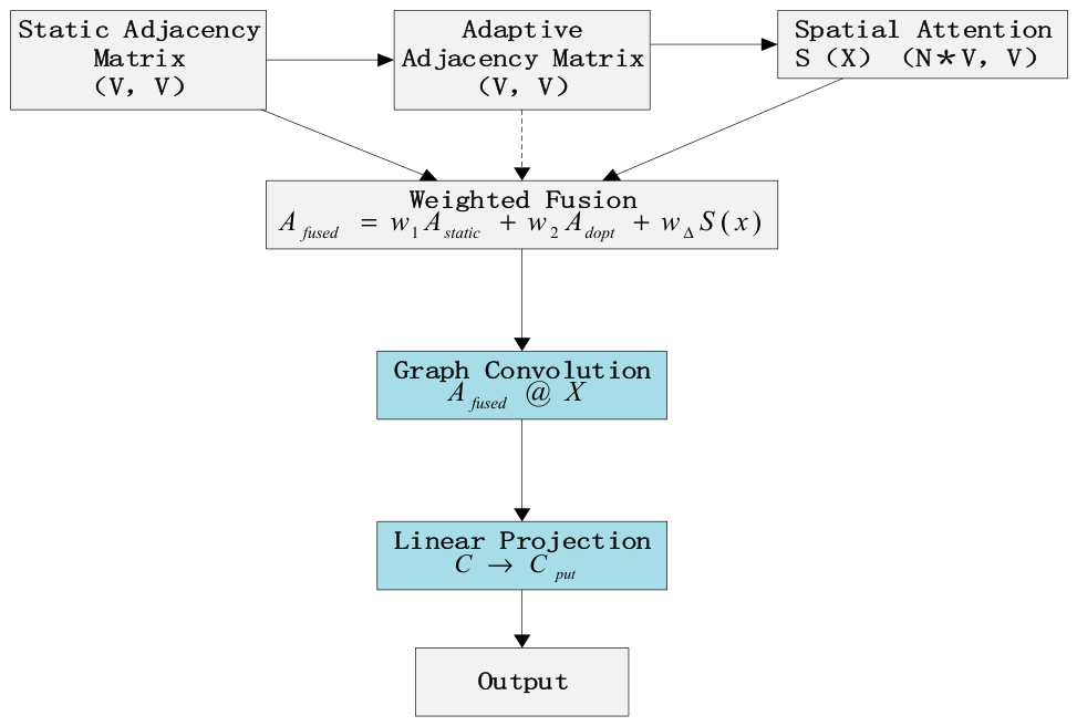
Figure 17.
Schematic of the Fusion Graph-Convolutional Architecture.
3. Results
3.1. Dataset Source and Preprocessing
The experimental data were collected from the traffic detection system of the Shizuizi Tunnel on the Jicao Expressway, including vehicle flow at the tunnel entrance and across different segments, which faithfully reflect the actual operating conditions of the tunnel.
During data preprocessing, outliers were removed and missing values were interpolated. The data were then normalized to improve training stability and convergence efficiency. Subsequently, samples were constructed using a sliding time window, where historical traffic flow data were used as inputs and future traffic flow as prediction targets. Meanwhile, traffic flow from each tunnel segment was mapped to graph node features to build a spatiotemporal graph dataset, providing support for subsequent modeling.
In addition, the distribution of traffic flow was analyzed, as shown in Figure 18. The results indicate that traffic flow values are mainly concentrated in the range of 0–1000, with the highest frequency observed in the 500–750 interval, exhibiting a right-skewed long-tailed distribution. This suggests that medium traffic flow states dominate, while high-flow samples are relatively scarce, providing a reliable data basis for model training and error analysis.
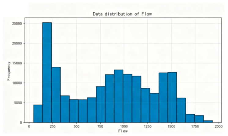
Figure 18.
Traffic Flow Data Distribution Chart.
3.2. Similarity Analysis of Traffic Flow Data
A similarity analysis of weekday (Monday–Friday) traffic data reveals consistent temporal patterns in tunnel traffic flow. As shown in Figure 19, traffic flow curves exhibit strong similarity across weekdays, with pronounced peaks during the morning (7:00–9:00) and evening (17:00–19:00) rush hours, while remaining relatively stable during off-peak periods. This temporal consistency reflects regular commuting demand and the dynamic response of tunnel traffic capacity, providing essential support for traffic state prediction and time-segmented control strategies.
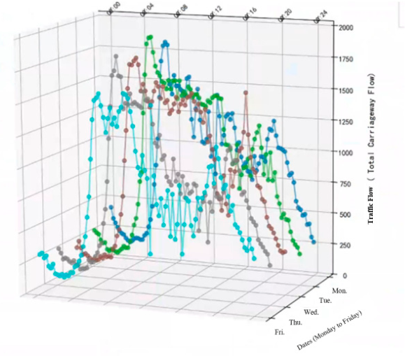
Figure 19.
Results of Traffic Operation Similarity Analysis for Highway Tunnels.
To analyze temporal similarity in traffic flow and vehicle speed, the Pearson correlation coefficient is adopted as a standard metric for linear correlation. It quantifies the similarity of traffic flow patterns across weekdays (Monday–Friday). The mathematical formulation is given below:
Pearson correlation analysis shows that correlation coefficients of traffic flow across weekdays range from 0.866 to 0.978 (Table 3), indicating strong overall consistency. The highest correlation is observed between Tuesday and Wednesday, followed by Thursday and Friday, while the correlation between Monday and Friday is relatively lower. These results confirm strong temporal similarity in weekday traffic flow, characterized by pronounced peaks during the morning (7:00–9:00) and evening (17:00–19:00) rush hours and relatively stable conditions during off-peak periods. Peak–trough fluctuations are highly synchronized across all weekdays. These patterns reflect regular commuter-dominated demand and temporal variations across different time intervals, providing a solid theoretical basis for tunnel traffic flow prediction and operational optimization.
Table 3.
Traffic Flow Similarity Results.
| Date | Monday | Tuesday | Wednesday | Thursday | Friday |
|---|---|---|---|---|---|
| Monday | 1 | 0.949 | 0.943 | 0.931 | 0.906 |
| Tuesday | 0.949 | 1 | 0.978 | 0.927 | 0.866 |
| Wednesday | 0.943 | 0.978 | 1 | 0.924 | 0.867 |
| Thursday | 0.931 | 0.927 | 0.924 | 1 | 0.954 |
| Friday | 0.906 | 0.866 | 0.867 | 0.954 | 1 |
3.3. Periodic Analysis of Traffic Flow Data
To investigate weekly periodicity in tunnel traffic flow, four representative weekdays (August 6, 13, 20, and 27), each separated by one week, are selected for analysis. As all selected dates fall on weekdays, the influence of weekend travel patterns is excluded, enabling a clearer characterization of weekly traffic regularity.
As shown in Figure 20, traffic flow curves exhibit highly consistent periodic patterns across the four dates, with pronounced peaks during the morning (7:00–9:00) and evening (17:00–19:00) rush hours and relatively stable conditions during off-peak periods. This consistent peak–trough pattern reflects stable commuter-dominated demand and the dynamic response of tunnel traffic capacity over time, providing strong support for traffic state prediction and time-segmented control strategies based on periodic characteristics.
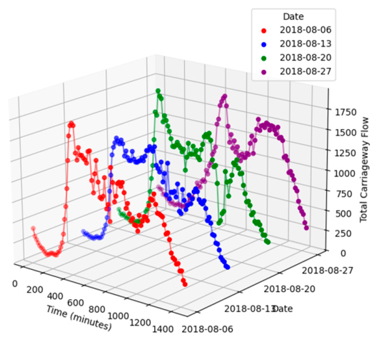
Figure 20.
Results of the Cyclical Nature of Highway Tunnel Traffic Operations.
Based on traffic flow data from four representative dates (August 6, 13, 20, and 27), pairwise Pearson correlation analysis is performed to construct a correlation matrix. The results indicate that the highest correlation occurs between August 6 and August 20, reflecting highly consistent traffic flow patterns. Strong positive correlations are also observed between August 6 and 13, as well as between August 13 and 20, indicating high similarity and stability in traffic flow across these dates.
In contrast, correlations involving August 27 are relatively lower compared with the other dates. Although moderate positive correlations are still observed, noticeable differences exist in their periodic fluctuation patterns. These findings confirm strong temporal consistency in traffic flow across most weekdays, reflecting stable commuter-driven demand. The relatively lower correlations on specific dates suggest that external factors may introduce structural variations, providing a reliable basis for traffic state prediction and anomaly detection.
Table 4.
Results of Traffic Flow Periodicity Analysis.
| Date | 8.6 | 8.13 | 8.20 | 8/27 |
| 8.6 | 1 | 0.821 | 0.945 | 0.523 |
| 8.13 | 0.821 | 1 | 0.809 | 0.477 |
| 8.20 | 0.945 | 0.809 | 1 | 0.516 |
| 8.27 | 0.523 | 0.477 | 0.516 | 1 |
3.4. Evaluation Metrics
This paper selects mean squared error (MSE), root mean square error (RMSE), and mean absolute percentage error (MAPE) as evaluation metrics. Mean squared error is one of the most commonly used loss functions in regression problems, used to measure the average squared difference between predicted and true values. Its formula is:
The root mean square error is:
The mean absolute percentage error is a common metric for measuring prediction accuracy, particularly suitable for scenarios where it is necessary to understand the proportion of prediction error relative to the actual value. Its formula is:
3.5. Analysis of Experimental Results
Before evaluating model performance, we first analyze the training process of FSE-ST-GCN. Figure 16 shows the loss curve during the training phase. As the number of training iterations increases, the loss value gradually decreases and stabilizes, indicating that the model can effectively learn the spatio-temporal features of traffic flow. The curve is generally smooth, indicating a stable training process.
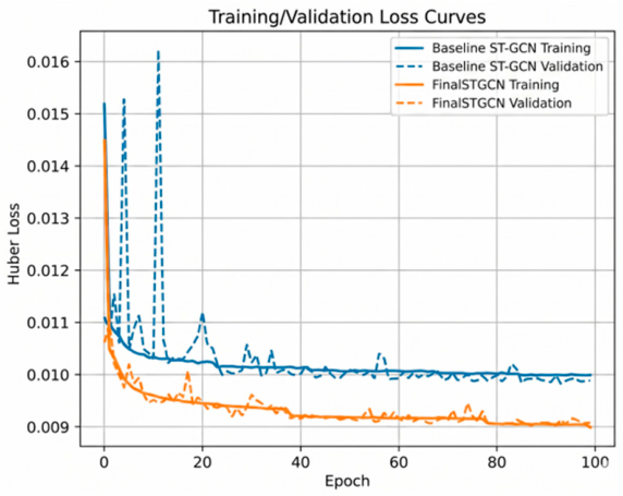
Figure 21.
Training loss curve of FSE-ST-GCN.
To evaluate the performance of the proposed FSE-ST-GCN model, comparative experiments are conducted against ST-GCN and several of its variants, as summarized in Table 5. The compared methods include the baseline ST-GCN, ST-GCN with an adaptive graph learning module that dynamically updates the graph topology, SE-ST-GCN that incorporates Squeeze-and-Excitation modules to enhance channel-wise feature recalibration, and Spatial Attention ST-GCN mechanisms for adaptive node importance weighting.
These variants represent representative advancements in spatio-temporal graph neural networks for traffic prediction and provide a comprehensive benchmark for evaluating the proposed model. The detailed results are presented in Table 3.
Table 5.
Summary of Model Comparisons.
| Model | MAE | RMSE | MAPE |
|---|---|---|---|
| ST-GCN | 55.720 | 88.342 | 7.790 |
| ST-GCN+Adaptive Graph | 55.465 | 85.311 | 8.049 |
| SE-ST-GCN | 54.507 | 86.620 | 7.619 |
| Spatial Attention ST-GCN | 55.372 | 85.574 | 7.754 |
| FSE-ST-GCN | 53.485 | 84.667 | 7.588 |
FSE-ST-GCN achieves the optimal performance across all evaluation metrics including MAE, RMSE, and MAPE, with corresponding values of 53.485, 84.667, and 7.588, respectively. In comparison with the baseline ST-GCN model, the proposed model consistently lowers prediction errors and enhances overall forecasting accuracy.
The experimental results demonstrate that each improved component contributes to performance promotion from different perspectives. Specifically, the adaptive adjacency matrix optimizes RMSE by strengthening spatial dependency modeling; the channel attention mechanism further reduces MAE and MAPE via improved feature discriminability; and the spatial attention module refines the modeling of inter-node spatial dependencies.
By comprehensively integrating all aforementioned mechanisms, FSE-ST-GCN surpasses all single-improvement variant models on every evaluation indicator. Relative to the original ST-GCN, the MAE, RMSE, and MAPE are reduced by 4.01%, 4.16%, and 2.59% respectively, which verifies the stable and effective performance enhancement of the proposed model.
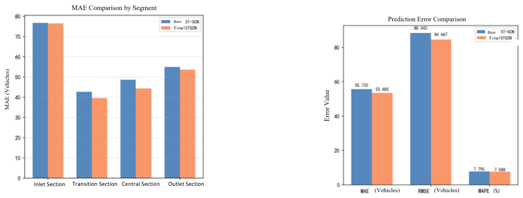
Figure 22.
FSE-ST-GCN Error Comparison Chart.
To further illustrate the model’s traffic flow prediction performance, typical traffic flow variations at multiple key monitoring points were selected for comparative analysis, as shown in Figures 23 to 26.
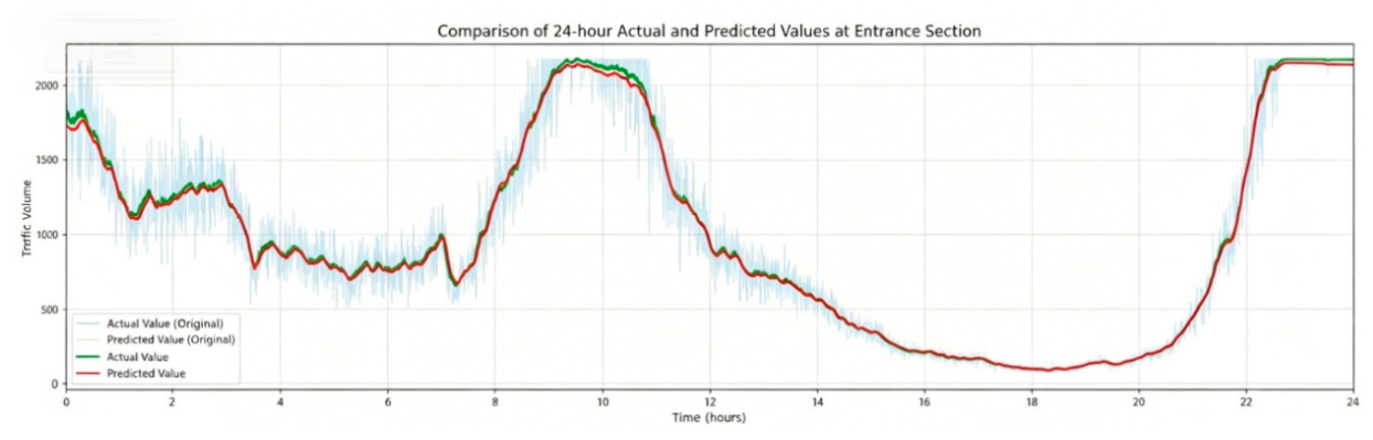
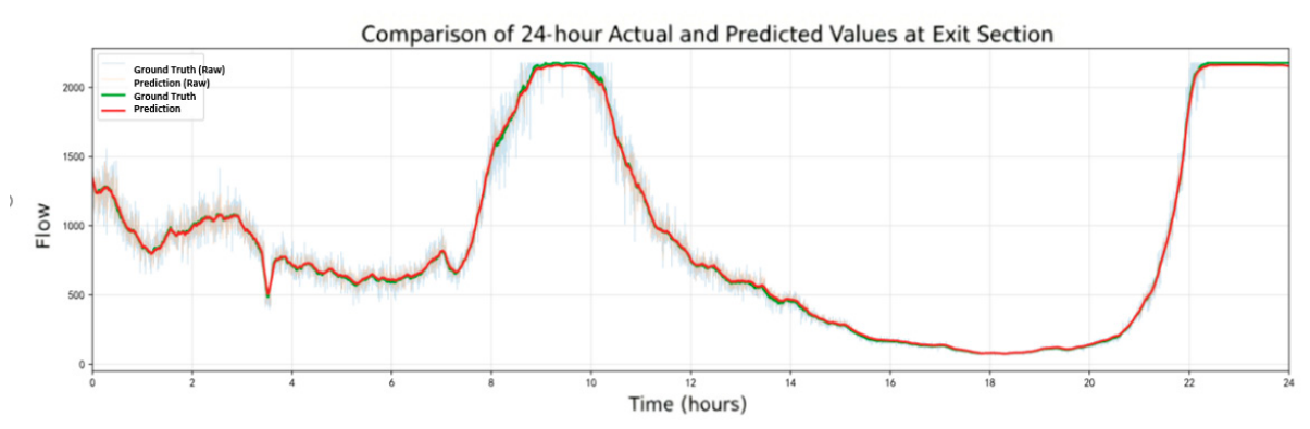
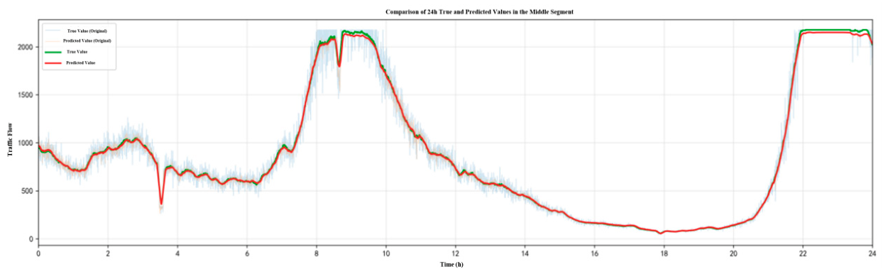
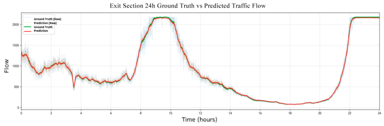
Figure 23.
Comparison of Inlet Segment Predictions for Tunnel Segments.
Figure 24.
Comparison of Tunnel Segment Predictions: Transition Section.
Figure 25.
Comparison of Predictions for the Middle Section of Tunnel Segments.
Figure 26.
Comparison of Tunnel Segment Predictions: Exit Section.
As shown in Figure 23, Figure 24, Figure 25 and Figure 26, the FSE-ST-GCN model yields prediction results that are closer to the actual traffic flow values and can better capture the fluctuating trends of traffic changes. During multi-step forecasting, the prediction error grows at a slower rate, which indicates the model possesses strong stability and reliability.
In summary, the integration of the adaptive adjacency matrix, channel attention mechanism, and spatial attention mechanism effectively enhances the model’s capability to capture the spatio-temporal characteristics of traffic flow. This not only improves the accuracy of traffic flow prediction but also enhances the model’s robustness, ensuring stable and reliable performance in various traffic scenarios.
4. Conclusions
This paper addresses the challenges of complex spatiotemporal dependencies and dynamically varying spatial relationships in tunnel traffic flow prediction by proposing a macro–micro collaborative two-stage framework. In the first stage, a GWO-GRU model is employed to predict incoming traffic flow at the tunnel entrance, providing reliable macro-level inputs for subsequent modeling. In the second stage, an FSE-ST-GCN model integrating an adaptive adjacency matrix with spatial and channel attention mechanisms is developed to achieve fine-grained spatiotemporal prediction of traffic flow within the tunnel.
By introducing a fusion mechanism for multi-source spatial relationships, the proposed method effectively captures dynamic spatial dependencies. In addition, the incorporation of multi-dimensional attention mechanisms enhances feature representation capabilities. Experimental results demonstrate that the proposed method outperforms baseline models in terms of MAE, RMSE, and MAPE, achieving superior accuracy, stability, and generalization performance.
In summary, the proposed framework significantly improves the performance of tunnel traffic flow prediction and provides effective support for intelligent tunnel traffic management and control. Future work will focus on multi-source data fusion and improving model robustness under complex traffic conditions.
Author Contributions
Conceptualization, Y.Y. and Z.C.; methodology, Y.Y. and Z.B.; software, Y.Y.; validation, Y.Y., Z.C. and Z.B.; formal analysis, Y.Y.; investigation, Y.Y. and Z.B.; resources, Z.C. and X.C.; data curation, X.C., Z.B., Z.T.C. and G.C.; writing—original draft preparation, Y.Y.; writing—review and editing, Z.C. and X.C.; visualization, Y.Y.; supervision, Z.C.; project administration, Z.C. All authors have read and agreed to the published version of the manuscript.
Funding
This research received no external funding.
Data Availability Statement
The raw traffic flow and electromechanical system operation data used in this study were obtained from the operation authority of the studied expressway tunnel and are not publicly available due to operational security and data privacy restrictions. Anonymized, aggregated data may be made available from the corresponding author upon reasonable request and with formal permission from the data provider.
Acknowledgments
The authors would like to thank the expressway tunnel operation and management team for their support in data collection and technical guidance throughout this research.:
Abbreviations
The following abbreviations are used in this manuscript:
| GWO | Grey Wolf Optimizer |
| GRU | Gated Recurrent Unit |
| GWO-GRU | Grey Wolf Optimizer Optimized Gated Recurrent Unit |
| ST-GCN | Spatio-Temporal Graph Convolutional Network |
| FSE-ST-GCN | Fusion of Squeeze-and-Excitation and Spatial Attention based Spatio-Temporal Graph Convolutional Network |
| SE | Squeeze-and-Excitation |
| SA | Spatial Attention |
| CNN | Convolutional Neural Network |
| LSTM | Long Short-Term Memory |
| MAE | Mean Absolute Error |
References
- Duan, Z.; Du, W. Research on tunnel traffic flow prediction and lighting control based on the GWO-LSTM model. Mod. Tunn. Technol. 2024, 61, 157–165. [Google Scholar]
- Chen, J.; He, J.; Wang, P.; et al. Short-term traffic flow prediction on expressways based on an intelligent optimization CNN model. Logist. Sci. Technol. 2026, 49, 113–116. [Google Scholar]
- Sun, Z.; Li, J.; Feng, Y. Research on intelligent traffic flow monitoring and prediction based on deep learning. Softw. Eng. 2024, 27, 13–16. [Google Scholar]
- Zhang, R.; Han, Y. Traffic flow prediction model based on attention mechanism spatio-temporal graph convolutional network on U.S. highways. Appl. Sci. 2026, 16, 559. [Google Scholar] [CrossRef]
- Su, L.; Huang, J.; Li, F. Adaptive graph convolution neural networks with spatial and frequency domain attention mechanism for traffic flow forecasting. Appl. Soft Comput. 2026, 197, 115156. [Google Scholar] [CrossRef]
- Yuan, C.; Tong, X.; Guo, H.; et al. GDLP-Net: A model for urban traffic flow prediction capturing global dynamic and local conduction features. J. Geoinf. Sci. 2026, 28, 1121–1136. [Google Scholar]
- Zhang, R.; Zhan, J.; Ding, W.; et al. FGT-Net: A multi-granular fuzzy fusion network for stable and explainable traffic flow forecasting. Fuzzy Sets Syst. 2026, 53, 109872. [Google Scholar] [CrossRef]
- Ye, R.; Tao, Y.; Ni, Q. STDGFN: A spatio-temporal dual-graph fusion network for traffic flow prediction. Appl. Intell. 2026, 56, 133. [Google Scholar] [CrossRef]
Disclaimer/Publisher’s Note: The statements, opinions and data contained in all publications are solely those of the individual author(s) and contributor(s) and not of MDPI and/or the editor(s). MDPI and/or the editor(s) disclaim responsibility for any injury to people or property resulting from any ideas, methods, instructions or products referred to in the content. |
© 2026 by the authors. Licensee MDPI, Basel, Switzerland. This article is an open access article distributed under the terms and conditions of the Creative Commons Attribution (CC BY) license (http://creativecommons.org/licenses/by/4.0/).
Copyright: This open access article is published under a Creative Commons CC BY 4.0 license, which permit the free download, distribution, and reuse, provided that the author and preprint are cited in any reuse.


