
Submitted:
08 May 2026
Posted:
09 May 2026
You are already at the latest version
Abstract
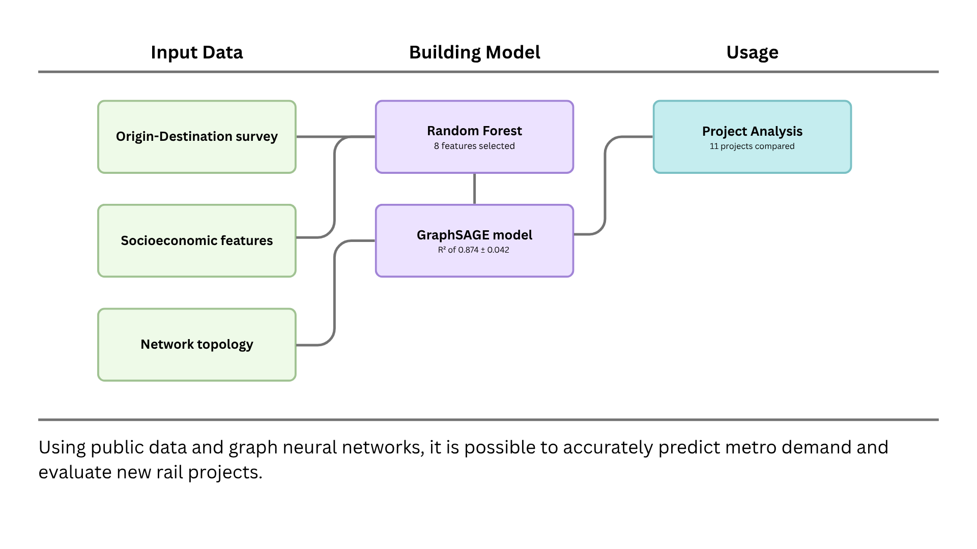
This work explores how graph theory concepts and neural networks can assist in strategic planning of metro network expansions using publicly available city data with the São Paulo Metropolitan Region. The methodology consolidated information from multiple public sources, developed a formula to estimate passenger demand based on catchment areas, applied Random Forest to identify the most relevant demographic features, and implemented a GraphSAGE model for demand prediction, extracting predictive capability from the topology of the system as well as socioeconomic features and Origin-Destination trips. The model achieved an R² of 0.874 ± 0.042 with minimal overfitting, outperforming the Random Forest approach. It can be applied to predict demand for future projects in a way that is accurate, inexpensive and computationally efficient, while also not requiring any rail system specific information besides topology. In this project, it was used to analyze multiple real projects and proposals for the São Paulo Metropolitan Region. Analysis revealed that employment, residences, and destinations where people go to eat represent 65% of the predictive capacity in the city.
Keywords:
graph neural networks
; urban planning
; urban rail transit
; graph theory
1. Introduction
The São Paulo metropolitan area is the most populous in the Western Hemisphere with a population of over 21.6 million people [1]. It is also a city with a growing rail system and falling number of passengers, even though the rail system is well approved [2,3,4]. Data from the Socioeconomic Characterization Survey of São Paulo Metro Users indicate that 66% of metro users own a car, and 75% of those who do not own a car say they would continue to use the metro even if they acquired a vehicle [5]. Furthermore, the metro was elected the Best Public Service in the city by Datafolha seven years in a row, up to the last survey in 2024 [6]. It is of note that in Brazilian studies cited in this paper, “metro” is a term that encompasses the subway, the metropolitan trains and the monorail. São Paulo also has high air pollution and studies show that expanding access to rail can significantly reduce the use of private vehicles [7,8,9]. The relationship between the number of vehicles and air pollution, combined with the preference of São Paulo residents for this mode of transport, highlights the potential impact of investments in the subway network. In this context, it is relevant to identify what drives rail usage and ways to help predict the demand for future projects.
The objective of this research is to offer a practical analysis that can contribute to the planning of the São Paulo subway system, assisting in strategic decision-making regarding the expansion of rail lines. The hypothesis is that it is possible to generate computationally inexpensive and reliable demand estimates to compare alternative projects using machine learning with graphs and publicly available city data aggregated into zones, without requiring any station data besides the topology of the system. By using only publicly available aggregated data, we hope to incentivize the public at large to engage in evaluating rail projects.
Traditional Graph theory offers a mathematical approach to modelling and analyzing public transportation networks, facilitating an understanding of the connectivity, efficiency, resilience and expansion potential of these rail networks [10,11]. Graph Neural Networks (GNN) represent an evolution in the application of deep learning techniques to graph-structured data, allowing both individual node and complex relational patterns in the network topology to be captured [12]. This approach is particularly relevant for transportation systems, where the spatial and functional relationships between stations can be as important as their individual characteristics [11,12].
Graph embeddings are a technique that converts graph structures into low-dimensional vector representations, making it possible to apply machine learning to graphs. Before the introduction of the Graph Sample and Aggregate (GraphSAGE) framework by Hamilton, Ying, and Leskovec in 2017, neural network architectures in graphs were mostly transductive, operating on static, predefined graphs where all nodes had to be present during embedding training [13]. GraphSAGE is the first framework capable of generating embeddings inductively. Rather than learning fixed embeddings for specific nodes, it learns an aggregator function that generates embeddings by sampling and aggregating features from local neighborhoods. This makes it capable of adding new nodes without complete retraining, making it much faster to test multiple scenarios [13]. Such an approach not only solves the scalability problem but also allows the capture of local structural patterns that can be generalized to different regions of the graph [14]. In the context of rail, GraphSAGE has been successfully applied for short-term origin-destination (OD) demand prediction using a multi-graph model titled mGraphSAGE, which predicts 20-minute interval passenger flows between stations based on real AFC (tap-in/tap-out) data [15]. It has also been used to model delay propagation across railway networks [16]. This thesis demonstrates how GraphSAGE can be adapted to predict metro ridership demand using only aggregated zone-level OD matrices and socioeconomic indicators, in the absence of station-to-station travel records. The method developed also makes it possible to use zone data to analyze specific station locations comprised of multiple zones in their catchment area and seamlessly considers network topology in its predictions, whilst being computationally efficient.
In order to use socioeconomic data to feed the GraphSAGE model, it was first necessary to select which features are the most impactful to avoid overfitting the model with excessive variables. For this purpose, Random Forest was selected. Random Forest is a machine learning algorithm that combines multiple decision trees to make predictions [17]. Each tree is trained with a random sample of the data and considers only a random subset of the variables in each split [17]. The final prediction is obtained by aggregating the results of all trees, either by majority vote (classification) or by average (regression), which reduces overfitting and increases the robustness of the model [17]. This method has been widely adopted for feature selection tasks due to its effectiveness in identifying critical features while discarding redundant information [18]. Feature selection through Random Forest offers four main advantages: simplifying the model by reducing the number of parameters, decreasing training time, reducing overfitting by enhancing generalization, and avoiding the curse of dimensionality [18]. It has also been shown to outperform other models when predicting modal travel choice [19,20].
With the GraphSAGE model created, it was possible to demonstrate its application in automated station selection through Monte Carlo Tree Search (MCTS), a general-purpose tree search algorithm that balances exploration and exploitation [21,22,23]. MCTS uses random simulations to guide search through the UCT (Upper Confidence bounds applied to Trees) algorithm [22,23]. This work uses the trained GraphSAGE model to evaluate network configurations during MCTS, with random rollout policies used for simulation phases. This implementation differs from recent sophisticated approaches like MetroZero, which integrates MCTS with self-play training, learned policy networks, and multi-objective optimization [24]. The simpler approach employed here serves to demonstrate that GraphSAGE ridership predictions contain sufficient information to guide automated expansion planning decisions.
2. Materials and Methods
In order to build and test the model, the first step was recreating the map of the complete rail network as it was in 2023, when the data for the most recent Origin Destination (OD) survey was compiled [25]. This task was made easier in part by using the Google Maps API, which allows addresses to be converted into coordinates. Each station was given a unique identifier. Next, the route of each line was written to map them as vertices in an initial topographic graph, which served to visually validate the coordinates of each station. Of the mapped stations, only four (Jundiaí, Campo Limpo Paulista, Várzea Paulista, and Botujuru) are located outside the OD survey coverage area and were therefore disregarded in the model.
The OD survey also captured 133 demographic, socioeconomic, and mobility features for each zone that were used in this study [25]. Demographic data include population by age group and gender, family structure, and number of households. Socioeconomic information covers education (from illiterate to higher education), income distributed into five brackets, car ownership, and occupational profile detailed by type of employment and economic sector (agriculture, industry, commerce, services, and public administration). Urban mobility is segmented by reason for travel, including work (by sector), education, shopping, health, leisure, job search, personal matters, meals, and residence, as well as information on public and private school enrolment.
Finally, information was collected on lines under construction, in the bidding process, in the study phase, and on expansions of existing lines. In cases where bidding documents were already published, the addresses were consolidated from the bids. Otherwise, it was necessary to analyze the maps of the project publications and manually find the addresses.
The collected features underwent correlation analysis to remove redundant variables and avoid overfitting. Next, feature selection was performed by a Random Forest using total subway and train trip data between zones for two reasons: the sample of zones is significantly larger than that of stations, and these values represent actual Origin and Destination (OD) survey data [25]. Based on this selection, the features values for each station are computed, as well as the volume of trips between pairs of stations. This data feeds a second Random Forest model, built to serve as a baseline for comparison with the GraphSAGE model. The latter seeks to estimate the number of trips between each pair of stations, using the same features selected in the previous step. Finally, the trained GraphSAGE model is applied to analyze subway network expansion projects. This entire pipeline is outlined in Figure 1.
In the Origin and Destination (OD) survey, the metropolitan region of São Paulo is divided into 527 zones of varying sizes [25]. For each zone, the relevant information available is the number of people who travel from that zone to each of the other zones, forming a square matrix of order 527, in which the zone of origin is the row and the zone of destination is the column. In this project, total trips are used to approximate the total possible demand, which is an acceptable simplification given that São Paulo has high subway ridership in the areas where it is built [5].
The challenge was to associate the zone information with current, under construction, and future stations. This task is not simple because the zones do not coincide with the area around the stations. In addition to zones with multiple stations, 111 of the 204 stations are less than 100 meters from a zone boundary, with an average distance to the centroid of 1,157.38 meters.
To approximate the number of trips between each two stations, some simplifications were made. First, it was considered that the distance people are willing to walk to a station, called Ped-Shed, is 882 meters, as it was found on the largest study we could find [26]. It is also assumed that people are distributed evenly throughout the space. That is, the percentage of the area covered is equal to the same percentage of trips to and from that area. When there is an intersection between Ped-Sheds, the area of the intersection is divided equally between the intersecting stations. Thus, (1) was considered for the total number of trips from any station x to any station y.
In which n is the number of zones in x, m is the number of zones in y, is the area of zone i that intersects with the area of station x, is the area of zone j that intersects with the area of station y, and is the number of trips from zone i to zone j.
Equation 1 enabled the creation of models that estimate the number of trips between stations based on actual data between zones. In addition, a greedy algorithm, called algorithm A, was developed to incrementally expand the number of stations. The algorithm works by systematically evaluating candidate locations around existing stations. For each station in the network, it generates candidates at specific distances and angles. The distances can be 1 km, 1.4 km, or 2.1 km, which are, respectively, the first quartile, the median, and the third quartile of the distances of all lines. Around each distance ring, candidates are positioned at 12 equidistant angles, essentially creating a circular pattern of potential locations every 30 degrees. To determine whether a candidate location improves the network, the algorithm recalculates the total number of passengers across the entire network. This involves calculating the number of passengers between each pair of stations, and for each pair, adding up the contributions of trips from all overlapping zones. For each alternative, all zone percentages for all stations are recalculated to ensure that overlaps are handled appropriately, and calculations are stored for the next iteration. The candidate that produces the highest total passenger demand on the network becomes the next permanent addition. Algorithm A has time complexity O().
One possible limitation of a model that attempts to use current urban mobility patterns to model demand for future projects is that mobility patterns depend on existing infrastructure. In addition, it is possible that features of each region are more predictive than current travel patterns. Therefore, a Random Forest was used to discover which attributes are most relevant and could assist in creating a model that can recommend new stations. It is important to mention that for the selection of attributes, all evaluations were made at the zone level, using the original values from the origin-destination survey. The target variable, also from the OD survey, is the sum of total subway and train trips between zones. Feature selection was performed at the zone level, as this allows for a larger sample size, 527 zones instead of 168 stations, and avoids creating false correlations through the aggregation process, since the method of transforming zone information into station information assumes that zones are homogeneous.
To select only the most relevant attributes and avoid overfitting, the first step was to select the variables with high correlation [27]. Spearman's correlation was selected for its robustness to non-normality and outliers [28]. Feature pairs with |ρ| > 0.70 and p < 0.05 were classified as correlated, following the commonly used threshold as the point where collinearity begins to severely distort model estimation [29]. The remaining variables were verified by interpreting their meaning before being used to make predictions, for example removing multiple subsections of jobs.
For the random forest, maximum tree depth was set to 6 to minimize overfitting. Feature selection robustness was validated using k-fold cross-validation, which partitions data into k subsets and iteratively trains on k-1 folds while testing on the remaining fold. Both k=5 and k=10 was evaluated, but had similar results. For each feature, two scores are created: Importance and Stability. Importance measures how much each feature reduces the impurity of the nodes when used for splits in all trees in the forest, with impurity being how homogeneous each group is. Stability measures the consistency of a feature's importance across different subsets of data, calculated using the coefficient of variation (CV). The stability score is calculated by taking the coefficient of variation, adding one to it, and then dividing one by that sum, creating a score between 0 and 1, where higher values indicate more stable features. The final selection of features uses a weighted combination, where 70% of the weight is assigned to average importance and 30% to importance weighted by stability, ensuring that the selected features are predictive and reliable.
The coefficient of determination (R²) measures the proportion of variance in the target variable explained by the model's predictions. The metric ranges from 0 to 1, where 1 indicates perfect prediction and 0 indicates that the model does not perform better than simply predicting the mean. Overfitting is quantified as the difference between the training R² and the test R². The Mean Absolute Error (MAE) calculates the average absolute difference between the predicted values and the actual values, providing an interpretable measure of the prediction error in the original units (subway trips).
The model was also used to find the zones of the city with the greatest potential for rail transport development. The result is a complete list of areas for which a station in that area could expect demand, which is the expected demand minus the supplied demand. The complete list is available on this project's GitHub.
Finally, the selected features are aggregated to the station level, considering that zones are homogeneous and the percentage of each zone that each station covers, similar to (1) for estimating the number of passengers. This makes it possible to assess how predictive these features are for estimating the number of trips between stations and to compare the Random Forest performance with the GraphSAGE model performance.
Next, a GraphSAGE neural network model was developed to predict passenger demand at potential future stations. The model combines the demographic and socioeconomic features selected by the Random Forest model with the network topology to predict demand patterns. To function at the station level, the value of each station feature was calculated as the sum of the contribution of each zone weighted by the percentage of coverage. For example, If Zone 100 has 10,000 jobs and Station 59 covers 80% of that zone, then Station 59 receives 8,000 jobs. The target variable is the daily passenger demand per station and was calculated using (1).
Unlike traditional machine learning approaches that treat stations as independent entities, GraphSAGE explores whether demand patterns at subway stations are influenced by their neighbouring stations in the network. The model processes this topological information using convolutional graph layers that aggregate information from neighbouring stations [13]. GraphSAGE learns a function that generates embeddings from sampling and aggregating features from the local neighbourhood of each node, enabling inductive generalization to nodes not seen during training [13]. Each station representation is iteratively refined by incorporating features from its directly connected neighbours [13].
The GraphSAGE architecture implemented consists of three convolutional graph layers with hidden dimensions of 64, 64, and 32, respectively. This configuration provides sufficient representational capacity through the initial expansion while using a moderate final dimension that may help prevent overfitting on the relatively small graph of 168 nodes. Between each layer, the model applies two operations that are crucial to its functioning. The ReLU activation function, which transforms negative values to zero while keeping positive values unchanged, adds essential nonlinearity to the model. Without this nonlinearity, multiple linear layers would be mathematically equivalent to a single linear transformation, capable only of learning affine relationships between features. Additionally, the 0.2 dropout randomly deactivates 20% of the units during each training iteration, preventing co-adaptation between neurons and forcing the model to develop robust representations that function reliably even when specific units are absent.
The trained GraphSAGE model was implemented to suggest potential expansions of the subway network. Algorithm A, described previously, needs to recalculate the total number of trips across the entire system to determine how much a new station would increase the total number of passengers. In comparison, algorithm B, based on MCTS using the GraphSAGE model, can generate new nodes without revisiting the entire graph. In addition, MCTS balances exploration and exploitation by using the Upper Confidence Bound (UCB) formula, allowing the algorithm to consider long-term rewards [23]. UCB assigns each candidate location a score that combines two factors: the average performance observed in previous simulations and an uncertainty bonus that favours locations that have not yet been fully explored [23]. This mechanism prevents the algorithm from prematurely settling on suboptimal solutions, ensuring a more comprehensive search of the space of possibilities [23].
3. Results
3.1. Estimating the Number of Passengers
Equation (1), described in section 3.4, was applied to the São Paulo rail network to see if the values were consistent with reality: The 2023 Origin and Destination Survey revealed that 15.3% of motorized trips in São Paulo were made by rail, with 11% by subway and 4.3% by train. It is important to note that the survey methodology uses a modal hierarchy: trips that include the subway and any other mode of transport are classified as “subway,” while trips by train (but without the subway) are classified as “train.” For example, a trip made by bus, train, and subway would be categorized as a subway trip. Applying (1) using the motorized trip matrix and a radius of influence of 882 meters around each station, we found that 15.15% of motorized trips could be made by rail. This result is remarkably close to the 15.3% observed in the survey. It makes sense that the calculated value is lower than the OD survey value because the latter does not capture multimodal trips in which other modes of transport are used to access stations, while the 15.3% survey value includes them. Some factors may be causing the value calculated by the formula to be higher and closer to the OD survey value: The 882-meter radius was derived from studies conducted in Nanjing, China, a city with urban characteristics that differ from those of São Paulo [25]. Nanjing has a lower population density, which may lead to lower expectations regarding public transportation services and greater acceptance of longer walks [30]. In addition, São Paulo has higher crime rates than Nanjing, which could reduce the willingness to walk long distances to stations [31,32].
Although (1) allows the number of trips on rails to be approximated from the total number of trips between zones, its application for network expansion is computationally costly. With each new station added, it is necessary to recalculate the spatial division of all stations to avoid overlaps and then recalculate the number of trips for all station pairs. Algorithm A, used to generate Figure 2, took 4 hours and 38 minutes to add 50 stations on a machine with an Apple M3 processor (12 cores), 18 GB of RAM, and MacOS 15.6.1. That makes for an average of 5 minutes and 33 seconds per stations. The Algorithm also gets slower the larger the graph, while the first station took 5 minutes and 18 seconds, the last station took 6 minutes and 23 seconds. That also means it would be even more inefficient for cities with larger rail networks. Despite the computational cost, the algorithm identified configurations that increase the total demand on the network by 65.0%, from 2,037,203 to 3,361,061 trips. The complete list of stations added with the demand gain caused by each of them can be found on this project's GitHub.
3.2. Feature Selection
The Random Forest for selecting features at the zone-level selected the 8 most relevant ones with a validation R² of 0.530 ± 0.029, an out-of-bag R² of 0.519 ± 0.014, and an MAE of 7360 ± 384. In this first zone-level model, rail coverage is not being taken into consideration. When it is, in the station-level analysis bellow, the predictive power increases substantially. Even so, an R² between 0.50 and 0.99 is acceptable in social science research, especially when most of the explanatory variables are statistically significant [33]. The only caveat is that high R-squared should not be caused by spurious causality or multicollinearity among the explanatory variables [34].
The analysis of attribute importance using Random Forest revealed a clear hierarchy of determinants of subway use, as seen in Table 1. The three dominant attributes, areas with Jobs (0.25), Residences (0.21), and Destinations people go to eat (0.20), together account for 65% of the model's predictive power. This demonstrates that subway demand in São Paulo follows commuting patterns between place of residence and place of work, with trips for meals emerging as the third significant component of this system. This result is consistent with total public transport trips being 53.55% for work [24]. The secondary attributes, with importance values between 0.05 and 0.08, demonstrate that socioeconomic factors and non-mandatory trips have a measurable but substantially smaller influence on demand prediction.
The Random Forest model using the features and the total number of trips between stations instead of zones achieved a coefficient of determination (R²) of 0.826 ± 0.037, representing a significant improvement over the zone-level model (R² = 0.530 ± 0.029). The overfitting index of 0.019 indicates good generalization capacity of the model, demonstrating that the difference between performance in training and validation data is minimal. This superior performance suggests that the formula used to transform the total number of trips and features into values between stations is an appropriate simplification.
3.3. GraphSAGE
The GraphSAGE model achieved an R² of 0.874 ± 0.042, demonstrating strong predictive power with remarkable consistency across folds. The model exhibited minimal overfitting with a training-test difference of only 0.004, comparing a training R² of 0.878 against a test R² of 0.874. Performance remained stable across all folds with test R² values ranging from 0.809 to 0.927, maintaining an average absolute error of 12,331 ± 2,139 trips per day. The consistency of performance with different data splits suggests that the model captures fundamental relationships between network structure, demographic characteristics, and demand patterns that are valid across the entire metro system.
Compared to the Station-Level Random Forest model, GraphSAGE demonstrates clear advantages, with R² increasing from 0.826 to 0.874. The fundamental difference between the approaches lies in how each model represents stations. Random Forest analyses each station in isolation, considering only its local characteristics, without incorporating information about its position in the network. GraphSAGE, on the other hand, represents each station in the context of its topological neighbourhood. The improvement in R² demonstrates that incorporating network topology provides substantial predictive value beyond isolated demographic characteristics. This result is consistent with a study that found a strong relationship between topological indicators, such as coverage, connectivity, and maximum number of transfers, and the demand for subway transportation in 19 systems around the world [11]. Metro stations are not independent entities, but components of an interconnected system, where demand patterns are shaped by the position and connectivity of each node.
Figure 3 shows subway network expansion generated by Algorithm B. Adding 50 new stations results in an estimated gain of 1,769,848 passengers (+27.2%). The colour scale represents the order of priority of stations by the algorithm, with warmer tones indicating stations selected in later iterations. The blue dashed lines correspond to the existing network, while the circular markers represent the stations proposed by the model.
Algorithm B demonstrated significantly higher computational efficiency than Algorithm A. To add 50 stations, Algorithm B took only 9 minutes whilst Algorithm A took more than 4 hours, both running on the same machine with an Apple M3 processor (12 cores). This difference increases with the number of stations due to the intrinsic characteristics of each approach: while Algorithm A, using (1), recalculates the total number of trips between each pair of existing stations and the new one, Algorithm B benefits from cumulative caching (as more simulations are performed, calculations of locations already visited are stored in memory) and the higher calculation speed of GraphSAGE. In isolated response time tests to evaluate 100 random coordinates, GraphSAGE is 2.74 times faster than (1), giving an average response of 0.44 ms compared to 1.20 ms. As a result, Algorithm B can add 200 stations in just 12.7 minutes, while an equivalent execution of Algorithm A would be computationally prohibitive. It should be noted that, as the methods for calculating gain differ between algorithms, although Algorithm B appears to result in a lower gain, this comparison does not necessarily indicate which approach identifies the best locations for deployment in the real world. Also, the GraphSAGE model has four fewer stations, given that the OD zones do not cover four stations in the system.
A consistent pattern emerged in the Algorithm B simulations: an initial preference for central regions of the city. This behaviour reflects the demographic reality of the São Paulo Metropolitan Region, where central areas have higher population density and concentration of economic activities. This result is consistent with the feature importance analysis of the Random Forest model. The complete list of added stations and the individual effect of each one is available in the project repository.
3.4. Future Lines
The application of the GraphSAGE model to evaluate existing expansion projects provides a quantitative tool for systematic comparison between different metro infrastructure proposals. Table 2 presents a comparative analysis of lines under construction, in the design phase, and expansions of existing lines. It was possible to identify not only the absolute gain of each project, but also its relative efficiency. For example, Line Celeste (19), currently being bided on, remarkably has the highest total impact, impact per station and impact per kilometer. It was also possible to note the high speed of the model, considering that none of the lines had an execution time of more than one second.
4. Discussion
This study addressed the challenge of assisting the planning of the expansion of the São Paulo Metropolitan Region subway network by applying concepts from graph theory and neural networks in graphs. A methodology was developed that combined the consolidation of data from multiple public sources, the creation of a formula to estimate passenger demand based on catchment areas, the selection of relevant characteristics using Random Forest, and the implementation of a GraphSAGE model for demand prediction. The attribute importance analysis revealed that jobs, residences, and destinations where people eat account for 65% of predictive capacity, confirming that subway demand in São Paulo follows typical commuting patterns.
The GraphSAGE model achieved an R² of 0.874 ± 0.042 with minimal overfitting of 0.004, significantly outperforming the baseline Random Forest approach which obtained an R² of 0.826. Results demonstrated that the proposed approach could generate reliable demand estimates and systematic comparisons between alternative projects while using only publicly available data. The ability of the GraphSAGE model to consistently evaluate different network configurations, considering both demographic characteristics and connection topology, enables planning decisions to be informed by comparable impact estimates. In addition, the speed of the model allows for the analysis of more alternatives. This is particularly relevant in contexts of limited resources, where it is necessary to prioritize among multiple expansion proposals with different characteristics of cost, extension, and location. Applying the model to evaluate eight real expansion projects allowed for quantitative comparisons using metrics such as total impact, efficiency per kilometer, and percentage improvement of the system.
However, this study has limitations that should be considered when interpreting the results and could serve as inspiration for future studies. The methodology developed focuses exclusively on maximizing passenger demand, without incorporating critical factors for implementation feasibility such as soil conditions, expropriation restrictions, construction costs per kilometer, technical feasibility of different routes, and environmental impacts. Real transportation planning decisions balance multiple objectives, including equity of access, regional economic development, and fiscal sustainability, which are not captured by the current model. In addition, the estimates assume that current mobility patterns will remain stable, not considering potential demographic changes, urban development induced by the expansion of the subway itself, or transformations in work patterns such as the increase in remote work. The demand estimation formula is based on a fixed catchment radius derived from studies in different urban contexts, when the willingness to walk to stations varies significantly depending on local characteristics such as safety, topography, and urban infrastructure. The model also does not consider integration with other modes of transportation. It would be possible to include trips made by people traveling to railway stations, or from stations to their destination, considering that in areas outside the Ped-Shed, a certain percentage of people travel to the nearest station. Finally, the analysis could benefit from data such as the capacity of each station and the speed of each line.
Author Contributions
Conceptualization, R.Z. and I.O.; methodology, R.Z.; software, R.Z.; validation, R.Z. and O.I.; formal analysis, R.Z.; investigation, R.Z.; data curation, R.Z.; writing—original draft preparation, R.Z.; writing—review and editing, R.Z. and O.I; visualization, R.Z.; supervision, O.I.; project administration, O.I.; Funding Acquisition, O.I; All authors have read and agreed to the published version of the manuscript
Funding
This research is part of the project "Development of a digital urban twin as an observatory of city dynamics to support sustainable planning and risk management" number 251009, supported by MACKENZIE RESEARCH AND INNOVATION FUND, called MACKPESQUISA. Then, this work was partly funded by the Mackenzie Research and Innovation Fund.
Data Availability Statement
The original data presented in the study are openly available in The Use of Graph Neural Networks in Rail Transport Planning at https://github.com/rafaelapz/The-Use-of-Graph-Neural-Networks-in-Rail-Transport-Planning. These data were derived from the following resources available in the public domain: https://www.metro.sp.gov.br/pesquisa-od/ and https://transparencia.metrosp.com.br.
Acknowledgments
The authors acknowledge Universidade Presbiteriana Mackenzie for the in-stitutional support that enabled the execution of this research and MACKENZIE RESEARCH AND INNOVATION FUND (MACKPESQUISA).
Conflicts of Interest
The authors declare no conflicts of interest.
References
- Renaux, P. População estimada do país chega a 213,4 milhões de habitantes em 2025. IBGE Agência de Notícias. 28 August 2025. Available online: https://agenciadenoticias.ibge.gov.br/agencia-noticias/2012-agencia-de-noticias/noticias/44305-populacao-estimada-do-pais-chega-a-213-4-milhoes-de-habitantes-em-2025.
- Número de passageiros de trem e metrô no País desacelera e transporte individual cresce em 2025. ANPTrilhos. 12 September 2025. Available online: https://anptrilhos.org.br/na-midia-numero-de-passageiros-de-trem-e-metro-no-pais-desacelera-e-transporte-individual-cresce-em-2025/.
- Metrô de SP: quais serão as próximas linhas e estações? Veja o cronograma das obras. O Estado de S.Paulo. 14 September 2024. Available online: https://anptrilhos.org.br/metro-de-sp-quais-serao-as-proximas-linhas-e-estacoes-veja-o-cronograma-das-obras/.
- Metrô é eleito novamente o Melhor Serviço Público de São Paulo. Metro SP. 2 May 2023. Available online: https://www.metro.sp.gov.br/2023/05/02/metro-e-eleito-novamente-o-melhor-servico-publico-de-sao-paulo/ (accessed on 6 August 2025).
- Companhia do Metropolitano de São Paulo. Pesquisa de Caracterização Socioeconômica dos Usuários e seus Hábitos de Viagem–2018; Companhia do Metropolitano de São Paulo: São Paulo, SP, Brazil, 2018. Available online: https://transparencia.metrosp.com.br/dataset/pesquisa-de-caracteriza%C3%A7%C3%A3o-socioecon%C3%B4mica-do-usu%C3%A1rio-e-seus-h%C3%A1bitos-de-viagem (accessed on 15 September 2024).
- Metrô e SUS são os vencedores na categoria Serviço Público. Folha de S.Paulo. 28 April 2025. Available online: https://www1.folha.uol.com.br/o-melhor-de-sao-paulo/2025/04/metro-e-sus-sao-os-vencedores-na-categoria-servico-publico.shtml (accessed on 8 November 2025).
- São Paulo real-world emissions study calls for national and city action to restrict dirty vehicles. TRUE Initiative. Available online: https://trueinitiative.org/insights/sao-paulo-study-calls-for-city-action/ (accessed on 6 November 2025).
- Zheng, S.; Zhang, X.; Sun, W.; Wang, J. The effect of a new subway line on local air quality: A case study in Changsha. Transp. Res. D. Transp. Environ. 2019, 68, 26–38. [Google Scholar] [CrossRef]
- Ye, X.; Sato, M. Impact of increased subway station density on air quality in the Yangtze River Delta. Environ. Res. Infrastruct. Sustain. 2023, 3, 035002. [Google Scholar] [CrossRef]
- Dees, B.S.; Xu, Y.L.; Constantinides, A.G.; Mandic, D.P. Graph theory for metro traffic modelling. In Proceedings of the International Joint Conference on Neural Networks (IJCNN), Shenzhen, China, 18–22 July 2021; pp. 1–5. [Google Scholar] [CrossRef]
- Derrible, S.; Kennedy, C. Network analysis of world subway systems using updated graph theory. Transp. Res. Rec. 2009, 2112, 17–25. [Google Scholar] [CrossRef]
- Rahmani, S.; Baghbani, A.; Bouguila, N.; Patterson, Z. Graph neural networks for intelligent transportation systems: A survey. IEEE Trans. Intell. Transp. Syst. 2023, 24, 8846–8885. [Google Scholar] [CrossRef]
- Hamilton, W.L.; Ying, R.; Leskovec, J. Inductive representation learning on large graphs. arXiv 2017, arXiv:1710.09471. [Google Scholar] [CrossRef]
- Ponzi, V.; Napoli, C. Graph neural networks: Architectures, applications, and future directions. IEEE Access 2025, 13, 62870–62891. [Google Scholar] [CrossRef]
- Nguyen, D.V.A.; et al. Multi-graph inductive representation learning for large-scale urban rail demand prediction under disruptions; Comput. Ind. Eng.: early access, 2024. [Google Scholar] [CrossRef]
- Li, Z.; Huang, P.; Wen, C.; Dong, W.; Ji, Y.; Rodrigues, F. Railway network delay evolution: A heterogeneous graph neural network approach. Appl. Soft Comput. 2024, 159, 111640. [Google Scholar] [CrossRef]
- Breiman, L. Random forests. Mach. Learn. 2001, 45, 5–32. [Google Scholar] [CrossRef]
- Chen, R.-C.; Dewi, C.; Huang, S.W.; Caraka, R.E. Selecting critical features for data classification based on machine learning methods. J. Big Data 2020, 7, 52. [Google Scholar] [CrossRef]
- Cheng, L.; Chen, X.; De Vos, J.; Lai, X.; Witlox, F. Applying a random forest method approach to model travel mode choice behavior. Travel Behav. Soc. 2019, 14, 1–10. [Google Scholar] [CrossRef]
- Wang, S.; Mo, B.; Zhao, J. Predicting travel mode choice with 86 machine learning classifiers: An empirical benchmark study. In Proceedings of the Transportation Research Board 99th Annual Meeting, Washington, DC, USA, 2020. [Google Scholar]
- Coulom, R. Efficient selectivity and backup operators in Monte-Carlo tree search. In Proceedings of the 5th International Conference on Computers and Games (CG 2006) Lecture Notes in Computer Science, Turin, Italy, May 2006; Springer: Berlin, Heidelberg, Germany, 2007; Vol. 4630, pp. 72–83. [Google Scholar] [CrossRef]
- Browne, C.B.; Powley, E.J.; Whitehouse, D.; Lucas, S.; Cowling, P.I.; Rohlfshagen, P.; Tavener, S.; Perez Liebana, D.; Samothrakis, S.; Colton, S. A survey of Monte Carlo tree search methods. IEEE Trans. Comput. Intell. AI Games 2012, 4, 1–43. [Google Scholar] [CrossRef]
- Kocsis, L.; Szepesvári, C. Bandit based Monte-Carlo planning. In Proceedings of the 17th European Conference on Machine Learning (ECML 2006) Lecture Notes in Computer Science, Berlin, Germany, 18–22 September 2006; Vol. 4212, pp. 282–293. [Google Scholar] [CrossRef]
- Alkilane, K.; Lee, D.-H. MetroZero: Deep reinforcement learning and Monte Carlo tree search for optimized metro network expansion. IEEE Trans. Intell. Transp. Syst. 2025, 26, 810–823. [Google Scholar] [CrossRef]
- Companhia do Metropolitano de São Paulo. Pesquisa Origem e Destino 2023; Companhia do Metropolitano de São Paulo: São Paulo, SP, Brazil, 2023. Available online: https://www.metro.sp.gov.br/pt_BR/pesquisa-od/ (accessed on 15 September 2024).
- Zhao, J.; Deng, W. Relationship of walk access distance to rapid rail transit stations with personal characteristics and station context. J. Urban Plan. Dev. 2013, 139, 311–321. [Google Scholar] [CrossRef]
- Ying, X. An overview of overfitting and its solutions. J. Phys. Conf. Ser. 2019, 1168, 022022. [Google Scholar] [CrossRef]
- Schober, P.; Boer, C.; Schwarte, L.A. Correlation coefficients: Appropriate use and interpretation. Anesth. Analg. 2018, 126, 1763–1768. [Google Scholar] [CrossRef] [PubMed]
- Dormann, C.F.; Elith, J.; Bacher, S.; Buchmann, C.M.; Carl, G.; Carré, G.; Diekötter, T.; García Márquez, J.R.; Gruber, B.; Lafourcade, B.; Leitão, P.J.; Münkemüller, T.; McClean, C.J.; Osborne, P.E.; Reineking, B.; Schröder, B.; Skidmore, A.K.; Zurell, D.; Lautenbach, S. Collinearity: A review of methods to deal with it and a simulation study evaluating their performance. Ecography 2013, 36, 27–46. [Google Scholar] [CrossRef]
- Vandebona, U.; Tsukaguchi, H. Impact of urbanization on user expectations related to public transport accessibility. Int. J. Urban Sci. 2013, 17, 199–211. [Google Scholar] [CrossRef]
- Kim, S.; Ulfarsson, G.F.; Hennessy, J.T. Analysis of light rail rider travel behavior: Impacts of individual, built environment, and crime characteristics on transit access. Transp. Res. A Policy Pract. 2007, 41, 511–522. [Google Scholar] [CrossRef]
- Tilahun, N.; Li, M. Walking access to transit stations: Evaluating barriers with stated preference. Transp. Res. Rec. 2019, 2534, 16–23. [Google Scholar] [CrossRef]
- Ozili, P.K. The acceptable R-square in empirical modelling for social science research. In Social Research Methodology and Publishing Results; IGI Global: Hershey, PA, USA, 2023; pp. 134–143. [Google Scholar] [CrossRef]
Figure 1.
Model creation pipeline.
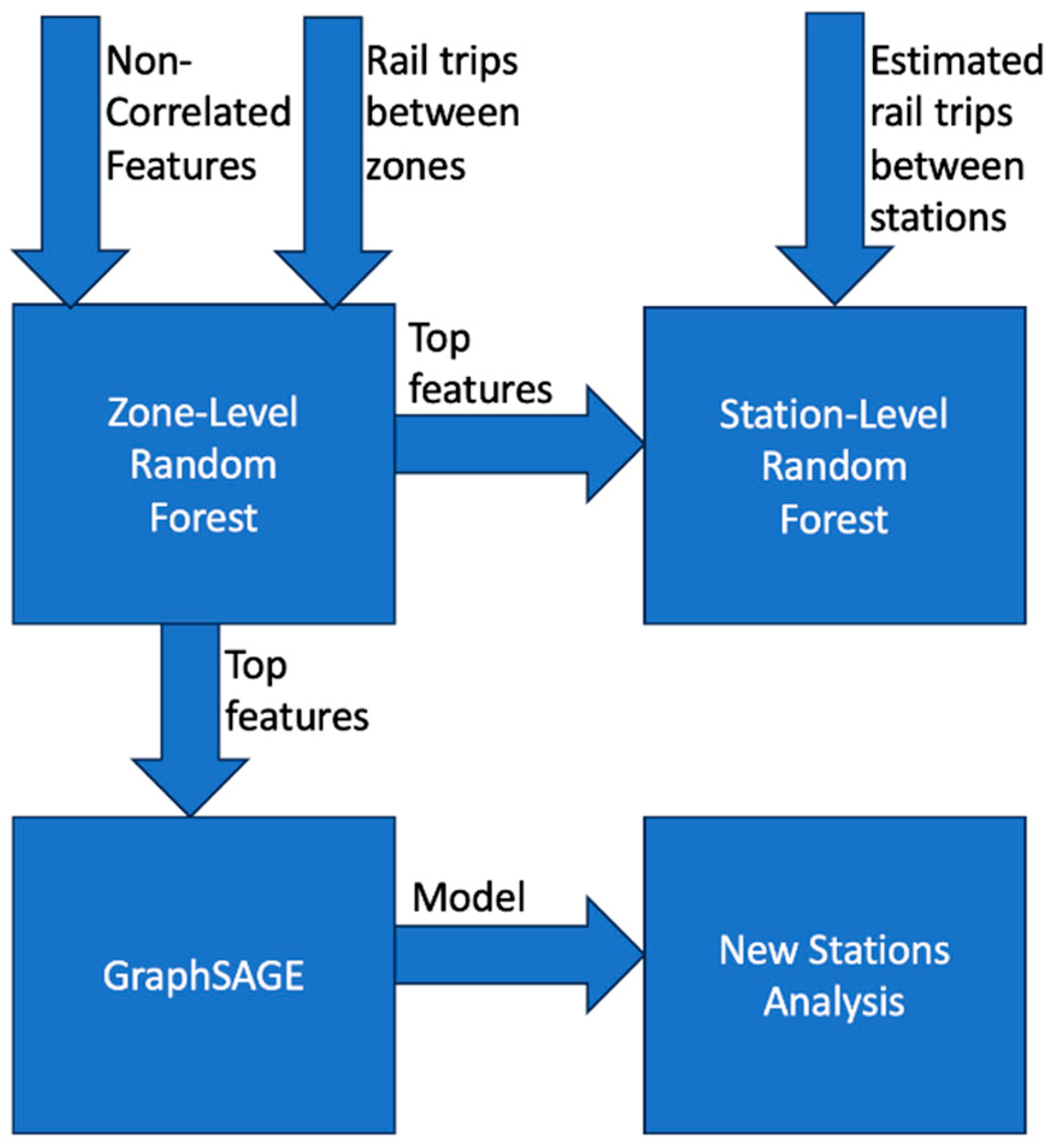
Figure 2.
Result adding 50 stations with Algorithm A. Algorithm A finds optimal locations from OD demand and does not care about topology. Therefore, edges connecting to new stations do not represent optimal lines, but show stations close enough to be connected to.
Figure 2.
Result adding 50 stations with Algorithm A. Algorithm A finds optimal locations from OD demand and does not care about topology. Therefore, edges connecting to new stations do not represent optimal lines, but show stations close enough to be connected to.
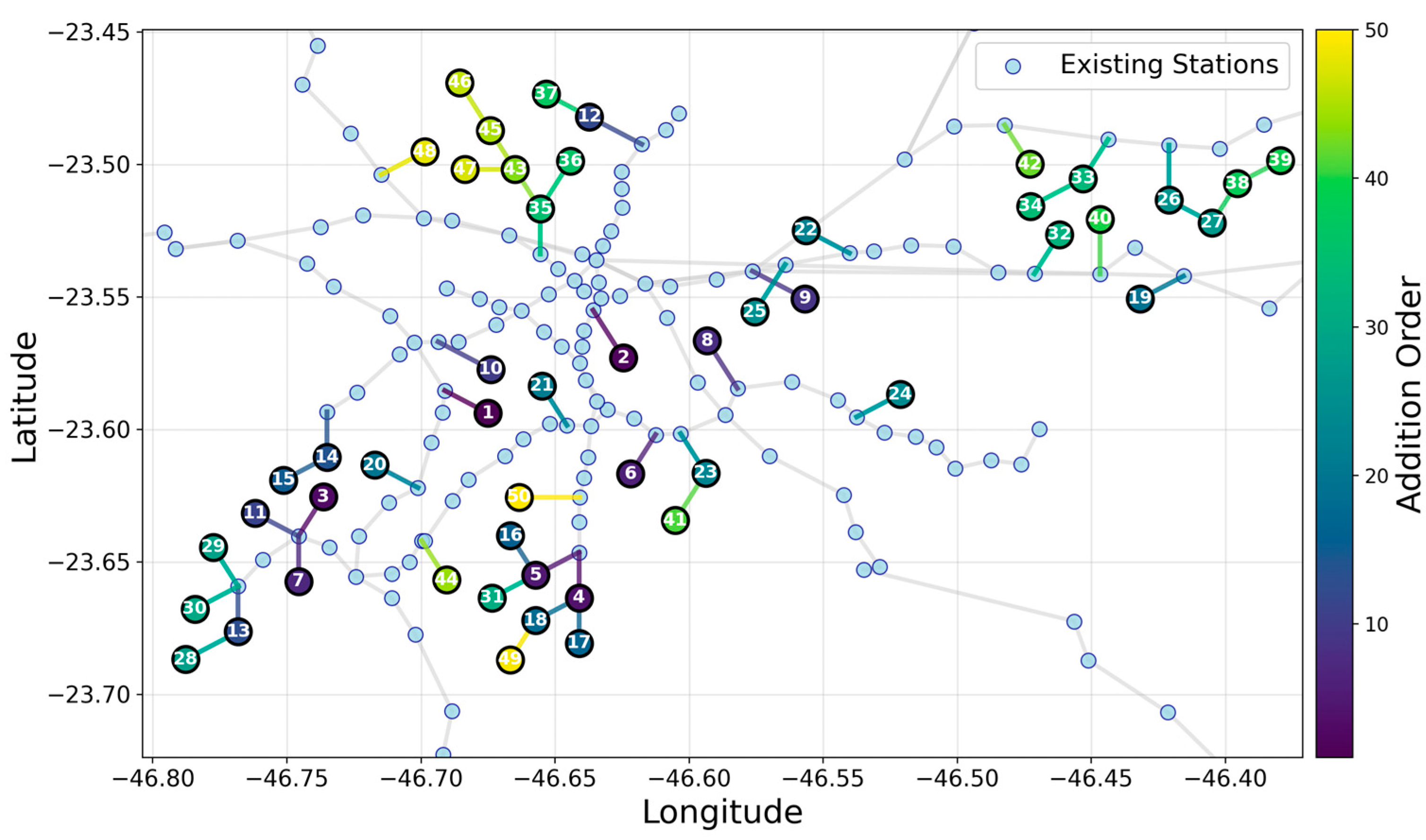
Figure 3.
Result adding 50 stations with Algorithm B.
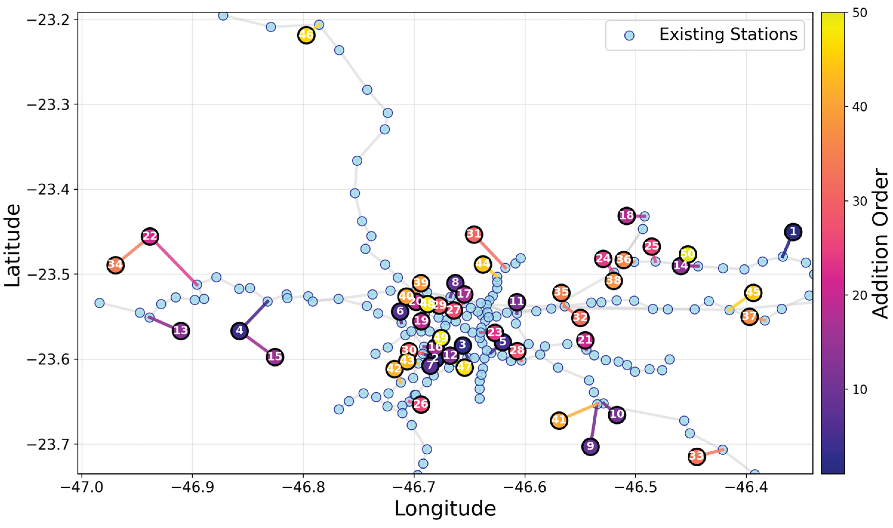

Table 1.
Top Features by Importance in Determining Rail Use
| Features | Importance | Stability |
|---|---|---|
| Jobs | 0.25 | 0.94 |
| Residences | 0.21 | 0.96 |
| Destination - food | 0.20 | 0.93 |
| Income up to R$ 2,640 | 0.08 | 0.92 |
| Destination - Personal Matters | 0.08 | 0.93 |
| Destination - Leisure | 0.07 | 0.93 |
| School enrolment | 0.07 | 0.89 |
| Destination - Health | 0.05 | 0.89 |
Table 2.
Comparison of multiple rail projects.
| Name | Status | Total Impact (trips/day) | System improvement (%) | Impact per Station | Impact per km | New Stations | Connections | Length (km) | Time (s) |
|---|---|---|---|---|---|---|---|---|---|
| Celeste (19) | Active Bidding | 2202245 | 34.85 | 146816 | 116262 | 13 | 2 | 18.9 | 0.9 |
| Violeta (16) | Prioritized by the government | 1389194 | 21.98 | 63145 | 39810 | 20 | 2 | 34.9 | 0.86 |
| Marrom (22) | Being planned | 1295150 | 20.45 | 68166 | 19487 | 17 | 2 | 66.5 | 0.84 |
| Laranja (6) | In construction | 875851 | 13.86 | 58390 | 67012 | 12 | 3 | 13.1 | 0.92 |
| Rosa (20) | Being planned | 837540 | 13.25 | 41877 | 21426 | 16 | 4 | 39.1 | 0.83 |
| Topazio (25) | Being planned | 227410 | 3.60 | 10829 | 5269 | 19 | 2 | 43.2 | 0.92 |
| Expansion Prata (15) – Jd. Colonial | In construction | 105332 | 1.67 | 15047 | 9755 | 6 | 1 | 10.8 | 0.87 |
| Expansion Verde (2) | In construction | 78016 | 1.23 | 9752 | 11348 | 7 | 1 | 6.9 | 0.79 |
| Expansion Ouro (5) | In construction | 76725 | 1.21 | 12788 | 19234 | 4 | 2 | 4 | 0.79 |
| Expansion Lilás (5) | In construction | 36108 | 0.57 | 12036 | 10122 | 2 | 1 | 3.6 | 0.78 |
| Expansion Amarela (4) | In construction | 19250 | 0.30 | 6417 | 4053 | 2 | 1 | 4.8 | 0.78 |
Disclaimer/Publisher’s Note: The statements, opinions and data contained in all publications are solely those of the individual author(s) and contributor(s) and not of MDPI and/or the editor(s). MDPI and/or the editor(s) disclaim responsibility for any injury to people or property resulting from any ideas, methods, instructions or products referred to in the content. |
© 2026 by the authors. Licensee MDPI, Basel, Switzerland. This article is an open access article distributed under the terms and conditions of the Creative Commons Attribution (CC BY) license (http://creativecommons.org/licenses/by/4.0/).
Copyright: This open access article is published under a Creative Commons CC BY 4.0 license, which permit the free download, distribution, and reuse, provided that the author and preprint are cited in any reuse.


