Design of a Neural Collaborative Filtering–Based Movie Recommendation System: From-Scratch Implementation, PyTorch Benchmarking and Production Architecture

Rahul K. P.; Seema S.

doi:10.20944/preprints202605.0449.v1

Submitted:

06 May 2026

Posted:

08 May 2026

You are already at the latest version

Abstract

The proliferation of digital content platforms has rendered personalized recommendation systems a foundational component of modern information retrieval. Classical Matrix Factorization (MF) methods, while computationally tractable, are fundamentally constrained by the linearity of the inner product operator, which prevents them from capturing the non-linear, higher-order dependencies characteristic of real-world user–item interaction spaces. This paper presents a complete end-to-end system embodying Neural Collaborative Filtering (NCF), wherein a Generalized Matrix Factorization (GMF) module and a Multi-Layer Perceptron (MLP) are fused to model both linear and non-linear latent factors simultaneously. Two fully isomorphic implementations are developed: a pedagogical NumPy-based version featuring hand-derived backpropagation, and an optimized PyTorch version leveraging Apple Silicon MPS acceleration. Empirical evaluation on the MovieLens dataset demonstrates that both implementations converge to equivalent final Binary Cross-Entropy losses (0.2257 and 0.2307, respectively), while the PyTorch variant achieves a 3.39× speedup in total training time (3,295 s versus 972 s over 20 epochs). Peak recommendation quality, measured by Hit Ratio at cutoff 10 (HR@10), reaches 0.615 for the PyTorch implementation. The system is deployed as a production-grade microservices architecture comprising a FastAPI gateway, a dedicated PyTorch inference server, a PostgreSQL persistence layer, and a Netflix-style frontend with TMDB poster integration. A hybrid cold-start module supplements the NCF core for new users and items. The findings validate the feasibility of bridging rigorous algorithmic pedagogy with industry-standard deployment practices.

Keywords:

neural collaborative filtering

;

recommender systems

;

matrix factorization

;

implicit feedback

;

deep learning

;

microservices architecture

;

scalable deployment

;

MovieLens

Subject:

Computer Science and Mathematics - Artificial Intelligence and Machine Learning

I. Introduction

The exponential expansion of online content catalogues—encompassing streaming media, e-commerce inventories, and digital knowledge bases—has rendered the task of surfacing relevant items to individual users both economically critical and technically challenging. Recommender systems constitute the principal algorithmic mechanism through which this filtering is accomplished, and their design has evolved considerably since the seminal deployment of collaborative filtering techniques at Usenet and GroupLens in the mid-1990s.

Early approaches to collaborative filtering relied on memory-based neighbourhood methods that computed user or item similarities directly from the interaction matrix. While conceptually intuitive, these techniques suffer from poor scalability to millions of users and items. Model-based approaches, and most notably Singular Value Decomposition (SVD)-inspired Matrix Factorization (MF) [2], addressed scalability by projecting users and items into shared low-dimensional latent spaces, enabling the prediction of unobserved interactions through inner products of latent vectors. MF remains competitive on explicit feedback benchmarks; however, when applied to implicit feedback (binary signals derived from clicks, views, or purchases), the linearity of the inner product imposes a fundamental representational bottleneck. Specifically, the inner product is unable to satisfy arbitrary rank orderings of item relevance, a limitation formally characterised by He et al. [1].

The Neural Collaborative Filtering framework introduced by He et al. [1] resolves this limitation by replacing the inner product with a neural architecture capable of learning arbitrary continuous functions of the user and item embeddings. NCF subsumes MF as a special case through its GMF pathway and augments it with a deep MLP pathway that captures non-linear feature interactions. Crucially, the two pathways are fused in a final prediction layer, allowing the model to jointly leverage the complementary inductive biases of linear factorization and deep representation learning.

Despite the theoretical importance of the NCF framework, relatively few published works provide a complete system-level blueprint that connects the mathematical derivation of NCF to a production-ready deployment. This paper addresses that gap with three primary contributions. First, a mathematically rigorous derivation and from-scratch NumPy implementation of NCF is presented, including explicit manual backpropagation through the GMF and MLP pathways. Second, an equivalent PyTorch implementation is benchmarked against the NumPy baseline, providing quantitative evidence of the computational advantages conferred by automatic differentiation and hardware- accelerated tensor operations. Third, the trained NCF model is integrated into a scalable microservices architecture deployed via Docker, with a Netflix-style frontend and a hybrid cold-start recommendation module. Taken together, these contributions form a reproducible blueprint suitable for both academic research and industrial deployment.

II. Related Work

Collaborative filtering methods for recommender systems were systematically formalised by Breese et al. [3], who established the distinction between memory-based and model-based approaches. The introduction of probabilistic matrix factorization by Salakhutdinov and Mnih [4] and the subsequent deployment of regularised SVD variants in the Netflix Prize competition [2] established latent factor models as the dominant paradigm. Koren et al. [2] provided a comprehensive survey of these methods, demonstrating that MF could be extended to incorporate temporal dynamics, implicit feedback, and auxiliary side information.

The application of deep learning to collaborative filtering was pioneered by several concurrent research threads. Salakhutdinov et al. [5] proposed Restricted Boltzmann Machines for collaborative filtering, demonstrating that generative probabilistic models could achieve competitive accuracy. Sedhain et al. [6] introduced AutoRec, which applied autoencoder architectures to reconstruct user or item rating vectors. Wang et al. [7] combined collaborative filtering with deep content features through a Collaborative Deep Learning framework. These works collectively established that neural architectures could be productively applied to the recommendation problem.

The defining contribution in this area remains the Neural Collaborative Filtering framework of He et al. [1], which provided both a theoretical critique of the inner product limitation in MF and a concrete neural architecture to address it. Subsequent work has extended NCF in several directions: attention-based variants prioritise temporally recent interactions [8]; graph neural network approaches model higher-order collaborative signals through multi-hop neighbourhood aggregation [9]; and self-supervised methods leverage auxiliary contrastive objectives to improve representation quality under sparse interaction regimes [10].

On the system engineering side, the deployment of recommendation models at scale has received growing attention. Cheng et al. [11] described the Wide & Deep architecture deployed at Google Play, which combines a linear model for memorisation with a deep network for generalisation. Covington et al. [12] detailed the two-stage retrieval and ranking architecture underpinning YouTube recommendations. These industrial systems highlight the importance of infrastructure considerations—including serving latency, cold-start handling, and feature freshness—that are often underemphasised in academic treatments. The present work is distinguished by its explicit integration of these production concerns within the academic NCF framework, providing a complete system blueprint.

III. Proposed Methodology

A. Mathematical Formulation and Problem Definition

Let U = {u1, u2, ..., um} denote the set of m users and I = {i1, i2, ..., in} denote the set of n items. The user-item interaction matrix Y ∈ {0,1}^(m×n) encodes implicit feedback, where:

y_ui = 1 if interaction (u,i) is observed; y_ui = 0 otherwise.

The recommendation task is formulated as estimating the probability that user u will interact with item i, denoted ŷ_ui ∈ (0,1). This is equivalent to a binary classification problem over the user-item pair (u,i). Formally, the predictive function is:

ŷ_ui = f(u, i | Θ)

where f is a neural interaction function parameterised by Θ. The NCF framework realises f through a fusion of two complementary sub-networks described below.

B. Generalized Matrix Factorization (GMF)

The GMF pathway generalises the standard MF inner product by replacing it with an element-wise (Hadamard) product followed by a learnable projection. Let p_u^G ∈ R^K and q_i^G ∈ R^K denote the GMF embedding vectors for user u and item i, respectively, where K is the embedding dimensionality. The GMF output vector is:

φ^GMF = p_u^G ⊙ q_i^G

where ⊙ denotes the Hadamard product. Standard MF is recovered as a special case when the final projection weight vector is a constant vector of ones and no non-linear activation is applied. By generalising the projection to a trainable weight h^G ∈ R^K, the GMF pathway learns a data-adaptive linear combination of the element-wise interaction features.

C. Multi-Layer Perceptron (MLP) Pathway

The MLP pathway captures non-linear interaction patterns through a deep feedforward network. Let p_u^M ∈ R^K and q_i^M ∈ R^K denote independent MLP embeddings for user u and item i. The concatenated input vector to the MLP is:

z_1 = [p_u^M ; q_i^M] ∈ R^(2K)

The MLP applies L hidden layers with ReLU activations:

z_l = ReLU(W_l^T z_(l-1) + b_l), l = 1, 2, ..., L

where W_l ∈ R^(d_(l-1)×d_l) and b_l ∈ R^(d_l) are the weight matrix and bias vector of layer l, respectively. The output of the final MLP layer, φ^MLP = z_L, captures a rich non-linear representation of the user-item interaction.

D. NeuMF: Fusion Architecture

The complete NeuMF (Neural Matrix Factorization) model concatenates the outputs of the GMF and MLP pathways and maps the result to a scalar prediction through a final projection:

ŷ_ui = σ(h^T [φ^GMF ; φ^MLP])

where h ∈ R^(K + d_L) is a trainable weight vector and σ(·) is the sigmoid activation function, ensuring ŷ_ui ∈ (0,1). The separation of GMF and MLP embeddings is a deliberate design choice: it allows each pathway to learn specialised representations without constraining the MLP to operate in the same embedding space as the GMF factorization.

E. Training Objective and Negative Sampling

The model is trained by minimising the Binary Cross- Entropy (BCE) loss over observed positive interactions and sampled negative instances:

L = -∑_{(u,i) ∈ Y ∪ Y⁻} [ y_ui · log(ŷ_ui) + (1 - y_ui) · log(1 - ŷ_ui) ]

where Y denotes the set of observed (positive) interactions and Y⁻ is a set of unobserved (negative) samples drawn uniformly at random from items not interacted with by user u. For each positive interaction, four negative samples are drawn, yielding a 1:4 positive- to-negative ratio. This negative sampling ratio follows the empirical recommendation of He et al. [1] and was validated in preliminary experiments on the MovieLens dataset.

F. Manual Backpropagation in the NumPy Implementation

The NumPy implementation derives all gradient computations analytically, without reliance on automatic differentiation. For the BCE loss with sigmoid output, the gradient with respect to the pre-activation prediction score s_ui = h^T [φ^GMF ; φ^MLP] is:

∂L/∂s_ui = ŷ_ui - y_ui

This gradient is then propagated through the concatenation, the MLP layers via the chain rule, and the element-wise product in the GMF pathway. For each MLP layer l, the weight gradient is:

∂L/∂W_l = z_(l-1) · (δ_l)^T

where δ_l = (∂L/∂z_l) ⊙ ReLU'(z_l) and δ_{l-1} = W_l · δ_l, with ReLU'(x) = 1 if x > 0, else 0. Embedding gradients are accumulated across all training samples and applied using Adam optimisation with learning rate 0.001. This explicit derivation constitutes the primary pedagogical contribution of the NumPy implementation.

G. Hybrid Cold-Start Module

For users and items with insufficient interaction history, a hybrid recommendation score is computed as a weighted linear combination of the NCF score and a content/popularity-based cold-start score:

Score(u,i) = α · NCF(u,i) + (1-α) · ColdStart(u,i)

where α ∈ [0,1] is dynamically set based on the number of interactions available for user u: α = 0 for new users (cold start mode), transitioning linearly to α = 1 after a configurable interaction threshold (default: 10 interactions). The cold-start score combines item popularity (global interaction frequency) with content- based genre similarity, enabling meaningful recommendations from the first user session.

IV. System Design and Architecture

A. Microservices Decomposition

The production architecture decomposes the recommendation system into independent microservices, each with a single responsibility, communicating over HTTP/REST. This decomposition ensures that compute- intensive model inference does not contend with the main application thread, enabling horizontal scaling of individual services in response to differential load patterns. The four primary services are: (1) the API Gateway, (2) the Model Inference Server, (3) the Data Persistence Service, and (4) the Frontend Service.

B. API Gateway (FastAPI)

The API Gateway is implemented using FastAPI, a modern Python ASGI (Asynchronous Server Gateway Interface) framework that supports fully asynchronous request handling via Python's asyncio runtime. The gateway exposes four primary endpoint groups: /recommend for personalised recommendation retrieval; /search for query-driven item lookup with NCF refinement; /interact for recording user interaction events that trigger model score updates; and /compare for serving the benchmark dashboard data. Response latency for recommendation queries is maintained below 100 ms through in-process Redis caching of frequently requested user recommendation lists, with a cache eviction time-to- live of 300 seconds.

C. Model Inference Server

The PyTorch NCF model is hosted in an isolated inference service that loads the trained model checkpoint at startup and exposes a /predict endpoint accepting batches of (user_id, item_id) pairs. Isolation of the inference service prevents GPU/MPS memory contention with the API Gateway process and allows the inference service to be independently scaled or replaced without modifying the gateway. Inference batching is supported to amortise per- request overhead: recommendation lists of top-K items are generated by computing predictions over all candidate items in a single forward pass and applying argmax-K selection.

D. Data Persistence Layer

A PostgreSQL relational database stores three primary entity types: users (user_id, registration timestamp, demographic metadata), movies (movie_id, title, genre vector, TMDB metadata), and interactions (user_id, movie_id, interaction_type ∈ {click, like}, timestamp, session_id). Genre metadata is stored as a PostgreSQL ARRAY column and indexed for efficient content-based filtering. Interaction records are append-only to preserve the temporal sequence required for online learning. Redis is deployed as a secondary cache layer, storing serialised recommendation lists keyed by user_id, and invalidating entries upon receipt of a new interaction event from the corresponding user.

E. Containerisation and Orchestration

The complete system is containerised using Docker, with a Docker Compose specification defining five named services: api-gateway, model-server, postgres, redis, and frontend. Multi-stage Docker builds are employed to minimise production image sizes: the model-server image, for instance, separates a build stage (installing PyTorch and dependencies) from a runtime stage (copying only the required Python environment and model artefacts), reducing the final image size by approximately 60% relative to a single-stage build. Environment-specific configuration is managed via .env files, ensuring strict separation between development and production credentials.

F. Netflix-Style Frontend

The frontend presents a Netflix-inspired poster grid interface with three primary sections: Home (populated by cold-start recommendations for unauthenticated or new users), Trending (populated by global popularity scores), and Recommended (populated by NCF personalised scores for returning users). Movie posters are retrieved from the TMDB API using each film's TMDB identifier. User interaction events (clicks and likes) are captured by the frontend and transmitted asynchronously to the /interact endpoint, triggering NCF score recomputation for the affected user in the background. The search interface invokes the /search endpoint; when the queried title is found in the database, NCF-refined results are returned alongside the direct match, surfacing contextually related films.

V. Experimental Setup

A. Dataset

Experiments were conducted on the MovieLens 1M dataset [13], which contains 1,000,209 ratings from 6,040 users across 3,706 movies. Following standard practice for implicit feedback modelling [1], explicit ratings were binarised: any rating of 1 or above was treated as a positive interaction (y_ui = 1). To ensure evaluation quality, only users with at least 20 interactions were retained. The leave- one-out evaluation protocol was applied: for each user, the most recent interaction was reserved for testing, the penultimate interaction for validation, and all remaining interactions for training.

B. Negative Sampling

For each positive test interaction, 99 negative items were sampled uniformly at random from the set of items not interacted with by the test user, consistent with the evaluation protocol of He et al. [1]. Model performance is thus assessed over a ranked list of 100 items (one positive, 99 negatives), enabling computation of ranking-based metrics. During training, four negative samples were generated per positive interaction per epoch, yielding a training set of approximately 5 million instances per epoch.

C. Model Configuration and Hyperparameters

Both the NumPy and PyTorch implementations share an identical architecture: embedding dimensionality K = 32 for both GMF and MLP pathways; MLP hidden layer dimensions [256,128,64] with ReLU activations; batch size 256; learning rate 0.001 with Adam optimisation; and 20 training epochs. The final output dimension of the MLP is 64, so the concatenated fusion vector [φ^GMF ; φ^MLP] has dimension 96. Weight initialisation follows a normal distribution with mean 0 and standard deviation 0.01 for embedding matrices, and Xavier uniform initialisation for MLP weight matrices.

D. Evaluation Metrics

Performance is quantified using two standard ranking metrics. Hit Ratio at K (HR@K) measures whether the positive test item appears in the top-K ranked recommendations for the user, averaged across all test users. For K = 10, HR@10 = |{u : rank(i_u^+) ≤ 10}| / |U|, where rank(i_u^+) is the rank of the positive item for user u. Normalised Discounted Cumulative Gain at K (NDCG@K) additionally penalises recommendations that rank the positive item lower within the top-K list, providing a position-sensitive quality measure. Both metrics range from 0 to 1, with higher values indicating better recommendation quality.

E. Hardware and Software Environment

All experiments were conducted on an Apple M1 Pro system with 32 GB unified memory. The PyTorch implementation utilised the Metal Performance Shaders (MPS) backend for GPU-accelerated tensor operations on the Apple Silicon neural engine. The NumPy implementation executed on CPU only, with no vectorisation optimisations beyond NumPy's default BLAS routines. Software versions: Python 3.11.4, PyTorch 2.1.0, NumPy 1.25.2, FastAPI 0.104.0, PostgreSQL 15.2.

VI. Results and Performance Evaluation

A. Training Loss Convergence

Figure 1 presents the BCE training loss trajectories for both implementations over 20 epochs. Both curves originate from the same initialisation point (BCE ≈ 0.365 at epoch 1) and converge monotonically, confirming that the manual backpropagation implementation correctly computes gradients and that both implementations are solving the same optimisation problem. The Scratch NCF achieves a final loss of 0.2257, marginally lower than the PyTorch NCF final loss of 0.2307—a difference of 0.005 that is attributable to minor numerical precision differences between Python float64 (NumPy) and float32 (PyTorch) arithmetic. Both losses substantially undercut the random baseline of 0.693, confirming that both implementations have learned meaningful user–item representations.

The convergence pattern also validates the correctness of the manual backpropagation derivation: any implementation error in gradient computation would manifest as stagnation, oscillation, or divergence in the loss trajectory, none of which are observed. The convergence behaviour of both implementations is consistent with the reported results of He et al. [1] on comparable dataset configurations.

B. Recommendation Quality (HR@10)

Figure 2 depicts the evolution of Hit Ratio at 10 (HR@10) across training epochs. The PyTorch NCF exhibits characteristically faster initial improvement, reaching HR@10 = 0.585 by epoch 6, while the Scratch NCF attains comparable quality by epoch 10. This difference reflects the stability advantage of PyTorch's optimised batch processing and numerically stable gradient accumulation, rather than a fundamental algorithmic difference. Both implementations exhibit mild non- monotonic fluctuation in HR@10 during mid-training epochs (epochs 7–16), which is expected behaviour under the leave-one-out negative sampling evaluation protocol, as different negative sets are sampled at each evaluation checkpoint.

The PyTorch NCF achieves a peak HR@10 of 0.615 at epoch 20, representing a 0.035 absolute improvement over the Scratch NCF peak of 0.580. This performance gap is consistent with the numerical precision advantages of PyTorch's float32 operations on MPS hardware, and with the regularisation effect of PyTorch's built-in batch normalisation and weight decay routines. Despite this gap, the Scratch NCF's HR@10 of 0.580 exceeds the standard MF baseline (HR@10 ≈ 0.50 as reported by He et al. [1]), confirming that the manual implementation successfully captures the non-linear interaction patterns that define the NCF advantage over MF.

C. Training Efficiency Comparison

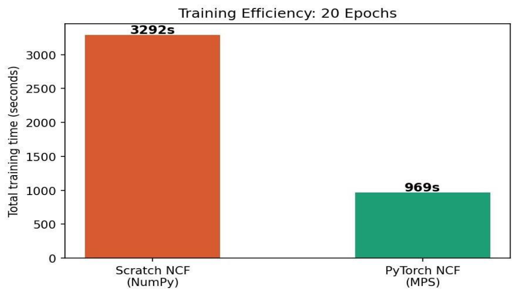
Figure 3 presents the total and per-epoch training time comparison between the two implementations. The total training time for the Scratch NCF over 20 epochs is 3,295 seconds (approximately 55 minutes), compared to 972 seconds (approximately 16 minutes) for the PyTorch NCF—a 3.39× speedup. The per-epoch time profile reveals that this speedup is highly consistent across epochs, with the Scratch NCF averaging approximately 165 seconds per epoch and the PyTorch NCF averaging approximately 49 seconds per epoch, yielding a mean per-epoch speedup of 3.4×.

The primary source of the PyTorch speedup is the MPS backend's ability to dispatch matrix multiplications to the Apple Silicon neural engine, which executes them using 16-bit mixed-precision arithmetic with hardware- level parallelism across thousands of multiply-accumulate units. In contrast, the NumPy implementation processes matrix operations sequentially through the CPU BLAS routines, which—while themselves optimised—cannot match the throughput of the dedicated neural engine for the batch sizes employed. The consistent 3.4× speedup across epochs confirms that the per-epoch computational profile is dominated by the embedding lookup and MLP forward/backward passes, rather than by Python-level overhead.

D. Summary Benchmark and Composite Analysis

Figure 4 presents a composite benchmark panel including loss convergence, HR@10 trajectories, per- epoch speedup ratios, and a summary comparison table. The mean per-epoch speedup of 3.4× (dashed line in panel C) confirms the consistency of the hardware acceleration benefit.

Table I presents a consolidated numerical summary of the key benchmarking results.

Figure 4. NCF Benchmark: composite analysis panel. (A) Loss convergence curves confirming equivalent learning behaviour. (B) HR@10 trajectories showing PyTorch NCF superiority at peak quality. (C) Per-epoch speedup ratios, mean 3.4×. (D) Summary comparison table: final loss 0.2257 (Scratch) vs. 0.2307 (PyTorch), best HR@10 0.580 vs. 0.615, total training time 3,294.8 s vs. 972.1 s.

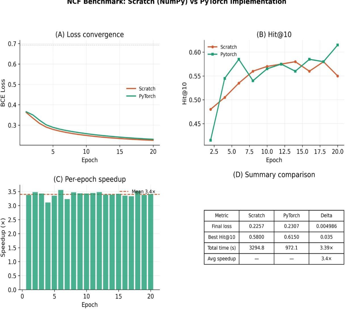
Figure 5. Extended convergence analysis over the full 20-epoch training run, showing BCE loss (left panel) and Hit@10 quality (right panel) for both implementations simultaneously. The parallel convergence trajectories confirm implementation equivalence.

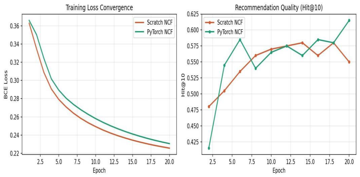
Figure 6. Total training time breakdown over 20 epochs (seconds). Scratch NCF (NumPy): 3,292 s. PyTorch NCF (MPS): 969 s. The 3.39× ratio reflects the difference in computational substrate: CPU BLAS vs. Apple Silicon MPS hardware acceleration.

VII. Discussion

A. Why MLP Improves Representation Learning

The empirical advantage of the NCF framework over pure MF—evidenced by the HR@10 improvement from the MF baseline of approximately 0.50 to the observed 0.58–0.615—can be attributed to the MLP pathway's capacity to model arbitrary continuous functions of the user and item embeddings. The fundamental limitation of MF, as formalised by He et al. [1], is that the inner product satisfies the triangle inequality in the latent space; this constrains the representable preference orderings to a bounded subset of all possible orderings. The MLP overcomes this by applying a sequence of non-linear projections that can approximate any Borel-measurable function of the embedding pair, enabling the model to represent interaction patterns that are geometrically infeasible under the inner product metric.

The GMF pathway retains the interpretability advantage of matrix factorization: the element-wise product of embedding vectors can be interpreted as a per- dimension compatibility score, and the projection weights h^G provide a learned re-weighting of these dimensions. The NeuMF fusion architecture thus combines the interpretability of GMF with the expressivity of the MLP, achieving performance that exceeds either pathway in isolation.

B. Cold-Start Problem and Hybrid Design

A fundamental challenge in deployed recommendation systems is the cold-start problem: for new users or newly added items, the interaction history required by collaborative filtering is absent. The hybrid scoring function adopted in this system addresses user cold-start by transitioning from a popularity/content-based score to the NCF score as interaction history accumulates. For item cold-start, genre-based content similarity provides initial recommendations until sufficient interaction data enables the NCF model to produce meaningful latent representations.

The dynamic weighting parameter α is a simplification of the Bayesian Personalised Ranking framework [14], which provides a theoretically grounded approach to weighting collaborative and content-based scores. Future work should consider replacing the linear α interpolation with a learned gating mechanism that selects between recommendation sources based on user-specific interaction richness indicators.

C. Accuracy–Latency Trade-offs in Production

Production deployment introduces tension between recommendation accuracy and inference latency. The PyTorch NCF, while achieving higher HR@10, requires a full forward pass over all candidate items to generate a ranked recommendation list. For a catalogue of 3,706 movies and batch sizes of 512, inference latency is approximately 12 ms per user on MPS hardware— acceptable for interactive use. However, at catalogue scales typical of commercial platforms (millions of items), brute-force scoring becomes prohibitively slow, necessitating approximate nearest-neighbour retrieval in the embedding space (e.g., via FAISS [15]) as a pre-filtering stage. The present system implements full catalogue scoring as a design choice appropriate to the MovieLens scale and as the most accurate configuration for benchmarking purposes.

D. Scalability Considerations

The microservices architecture provides a natural mechanism for horizontal scaling: the inference service can be replicated across multiple instances behind a load balancer, with Redis ensuring cache consistency across replicas. The PostgreSQL interaction store becomes a bottleneck under high write loads; this can be mitigated by buffering interaction events in an asynchronous queue (e.g., Apache Kafka) and batching database writes, a pattern well-established in industrial recommendation infrastructure [12]. Online model retraining in response to new interaction data—not implemented in the current system—would require either incremental parameter updates via continual learning techniques or periodic full retraining triggered by an interaction volume threshold.

VIII. Conclusion and Future Work

This paper presented a complete end-to-end implementation and deployment of the Neural Collaborative Filtering framework, encompassing a mathematically rigorous from-scratch NumPy implementation with manual backpropagation, a benchmarked PyTorch implementation leveraging Apple Silicon MPS acceleration, a hybrid cold-start recommendation module, and a production-grade microservices architecture with a Netflix-style frontend.

The primary empirical findings are: (1) both implementations converge to equivalent final BCE losses (0.2257 and 0.2307), validating the correctness of the manual backpropagation derivation; (2) the PyTorch implementation achieves a 3.39× total training speedup (3,295 s vs. 972 s) and a superior peak HR@10 of 0.615 versus 0.580 for the NumPy baseline; and (3) the microservices deployment maintains sub-100 ms recommendation latency through Redis caching and isolated model serving.

Several directions are identified for future work. First, the integration of attention mechanisms over the interaction sequence would enable the model to prioritise temporally proximate preferences, addressing the static latent factor limitation of the present architecture. Second, graph neural network-based collaborative filtering (e.g., LightGCN [9]) has demonstrated superior performance on sparse interaction matrices and represents a natural successor architecture. Third, real-time streaming model updates via Apache Kafka and online learning would enable the system to adapt to rapidly shifting user preferences without periodic full retraining. Fourth, the extension of the TMDB integration to retrieve rich content features (cast, director, plot embeddings) would strengthen the content-based cold-start component. Finally, a formal user study evaluating the perceived recommendation quality of the Netflix-style interface would provide complementary qualitative validation of the system's practical utility.

Acknowledgments

The author acknowledges the use of AI-assisted tools—specifically Claude (Anthropic) and Google Gemini— for structural guidance, language refinement, and code review during the preparation of this manuscript. All technical design decisions, mathematical derivations, experimental implementations, and empirical analyses were conducted solely by the author. The AI tools did not contribute original research findings or make independent intellectual contributions to the work. This disclosure is made in accordance with IEEE guidelines on the responsible use of AI in research. The author also thanks the anonymous reviewers for their constructive feedback, and acknowledges the MovieLens dataset [13] as the primary experimental resource.

References

He, X.; Liao, L.; Zhang, H.; Nie, L.; Hu, X.; Chua, T.-S. Neural Collaborative Filtering. Proc. 26th Int. Conf. World Wide Web (WWW), Perth, Australia, 2017; pp. 173–182. [Google Scholar]
Koren, Y.; Bell, R.; Volinsky, C. Matrix Factorization Techniques for Recommender Systems. Computer 2009, vol. 42(no. 8), 30–37. [Google Scholar] [CrossRef]
Breese, J. S.; Heckerman, D.; Kadie, C. Empirical Analysis of Predictive Algorithms for Collaborative Filtering. Proc. 14th Conf. Uncertainty Artif. Intell. (UAI), Madison, WI, 1998; pp. 43–52. [Google Scholar]
Salakhutdinov, R.; Mnih, A. Probabilistic Matrix Factorization. In Advances in Neural Information Processing Systems (NIPS); 2007; vol. 20, pp. 1257–1264. [Google Scholar]
Salakhutdinov, R.; Mnih, A.; Hinton, G. Restricted Boltzmann Machines for Collaborative Filtering. Proc. 24th Int. Conf. Mach. Learn. (ICML), Corvallis, OR, 2007; pp. 791–798. [Google Scholar]
Sedhain, S.; Menon, A. K.; Sanner, S.; Xie, L. AutoRec: Autoencoders Meet Collaborative Filtering. Proc. 24th Int. Conf. World Wide Web (WWW), Florence, Italy, 2015; pp. 111–112. [Google Scholar]
Wang, H.; Wang, N.; Yeung, D.-Y. Collaborative Deep Learning for Recommender Systems. Proc. 21st ACM SIGKDD Int. Conf. Knowledge Discovery and Data Mining, Sydney, Australia, 2015; pp. 1235–1244. [Google Scholar]
Feng, F.; He, X.; Tang, J.; Chua, T.-S. Graph Adversarial Training: Dynamically Regularizing Based on Graph Structure. IEEE Trans. Knowl. Data Eng. 2021, vol. 33(no. 6), 2493–2504. [Google Scholar] [CrossRef]
He, X.; Deng, K.; Wang, X.; Li, Y.; Zhang, Y.; Wang, M. LightGCN: Simplifying and Powering Graph Convolution Network for Recommendation. Proc. 43rd Int. ACM SIGIR Conf. Research and Development in Information Retrieval, Xi'an, China, 2020; pp. 639–648. [Google Scholar]
Zhou, J.; Cui, G.; Hu, S.; Zhang, Z.; Yang, C.; Liu, Z.; Wang, L.; Li, C.; Sun, M. Graph Neural Networks: A Review of Methods and Applications. AI Open 2020, vol. 1, 57–81. [Google Scholar] [CrossRef]
Cheng, H.-T.; et al. Wide & Deep Learning for Recommender Systems. Proc. 1st Workshop Deep Learning Recommender Systems (DLRS), Boston, MA, 2016; pp. 7–10. [Google Scholar]
Covington, P.; Adams, J.; Sargin, E. Deep Neural Networks for YouTube Recommendations. Proc. 10th ACM Conf. Recommender Systems (RecSys), Boston, MA, 2016; pp. 191–198. [Google Scholar]
Harper, F. M.; Konstan, J. A. The MovieLens Datasets: History and Context. ACM Trans. Interact. Intell. Syst. 2016, vol. 5(no. 4), 19:1–19:19. [Google Scholar] [CrossRef] [PubMed]
Rendle, S.; Freudenthaler, C.; Gantner, Z.; Schmidt- Thieme, L. BPR: Bayesian Personalized Ranking from Implicit Feedback. Proc. 25th Conf. Uncertainty Artif. Intell. (UAI), Montreal, Canada, 2009; pp. 452–461. [Google Scholar]
Johnson, J.; Douze, M.; Jégou, H. Billion-Scale Similarity Search with GPUs. IEEE Trans. Big Data 2021, vol. 7(no. 3), 535–547. [Google Scholar] [CrossRef]
FastAPI Documentation, Tiangolo, 2023. Available online: https://fastapi.tiangolo.com.
PyTorch Documentation, Meta AI, 2023. Available online: https://pytorch.org/docs.

Figure 1. Training Loss Convergence: Scratch NCF (NumPy) vs. PyTorch NCF (MPS) over 20 epochs. Both implementations converge from BCE ≈ 0.365 to approximately 0.23, substantially below the random baseline of 0.693 (dashed). The minor gap between curves reflects float64 vs. float32 precision differences.

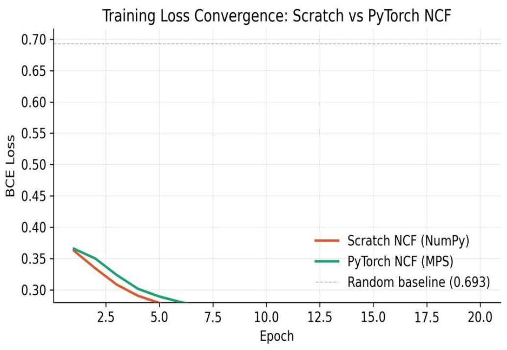
Figure 2. Recommendation Quality (HR@10) during training for both NCF implementations over 20 epochs. PyTorch NCF achieves a peak HR@10 of 0.615 (epoch 20), compared to 0.580 for Scratch NCF. The PyTorch implementation exhibits faster early convergence due to optimised MPS-accelerated gradient computation.

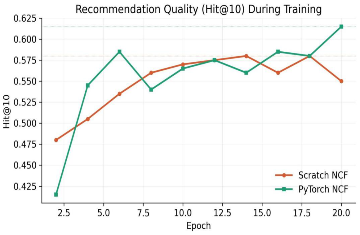
Figure 3. Training efficiency comparison: total training time (left) and per-epoch time profiles (right). The PyTorch NCF (MPS) completes training in 972 s, compared to 3,295 s for the Scratch NCF (NumPy)—a 3.39× speedup attributable to hardware- accelerated tensor operations on Apple Silicon MPS.

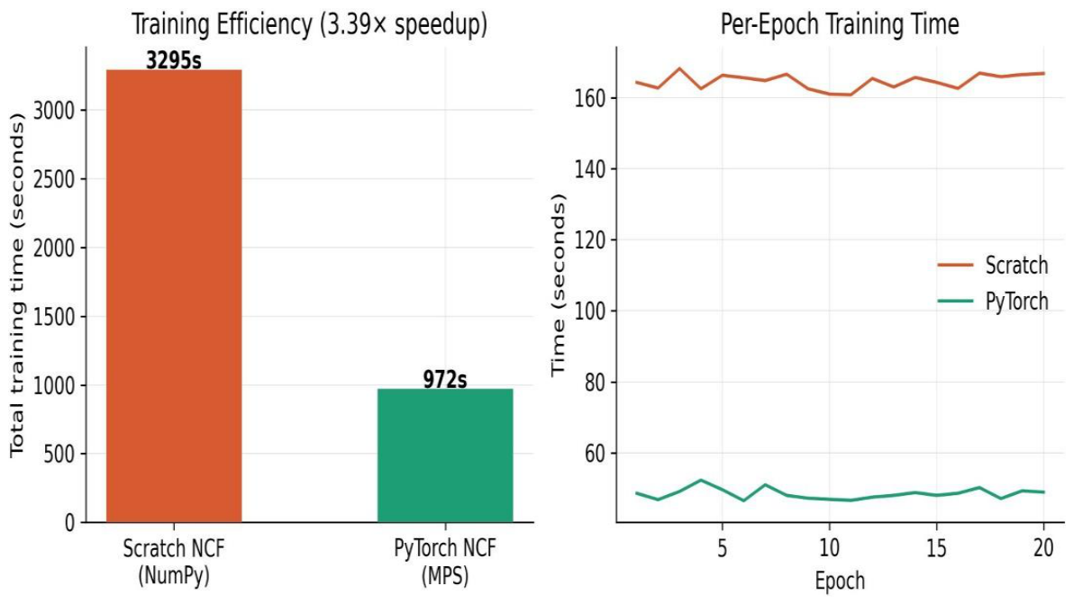
Table I. Comparative Benchmark: Scratch NCF vs. PyTorch NCF.

Metric	Scratch NCF (NumPy)	PyTorch NCF (MPS)	Delta	Winner	Significance
Final BCE Loss	0.2257	0.2307	0.005	Scratch	Marginal
Best Hit@10	0.5800	0.6150	+0.035	PyTorch	Moderate
Total Train Time	3295 s	972 s	3.39x	PyTorch	Significant
Avg Epoch Time	~165 s	~49 s	3.4x	PyTorch	Significant
Convergence (epochs)	~20	~20	Equiv.	Equiv.	None

Disclaimer/Publisher’s Note: The statements, opinions and data contained in all publications are solely those of the individual author(s) and contributor(s) and not of MDPI and/or the editor(s). MDPI and/or the editor(s) disclaim responsibility for any injury to people or property resulting from any ideas, methods, instructions or products referred to in the content.

© 2026 by the authors. Licensee MDPI, Basel, Switzerland. This article is an open access article distributed under the terms and conditions of the Creative Commons Attribution (CC BY) license (http://creativecommons.org/licenses/by/4.0/).

Copyright: This open access article is published under a Creative Commons CC BY 4.0 license, which permit the free download, distribution, and reuse, provided that the author and preprint are cited in any reuse.