
Submitted:
22 April 2026
Posted:
23 April 2026
You are already at the latest version
Abstract
Numerical simulation of the multi-dimensional space-fractional Cahn-Hilliard equation faces two main computational challenges: the inherent temporal accuracy limitations of standard scalar auxiliary variable (SAV) methods and the escalating computational cost in high-dimensional domains. To address these issues, this study constructs a fully discrete algorithmic framework integrating a second-order backward differentiation formula (SAV-BDF2) with a sixth-order centered difference scheme. Under this formulation, we rigorously prove unconditional energy stability and establish the theoretical validity of the dual temporal and spatial accuracy. To solve the resulting indefinite algebraic systems, a minimal residual solver is paired with a sine-transform block diagonal preconditioner. Additionally, a hardware-level Vectorized Tensor Processing (VTP) architecture is deployed to resolve cache thrashing caused by non-contiguous memory access during multidimensional tensor evaluations. Numerical experiments in 3D to 8D domains demonstrate that the framework improves memory throughput and reduces execution time. By avoiding standard hardware execution inefficiencies, this integrated strategy provides an efficient numerical solution for large-scale simulations of high-dimensional fractional systems.
Keywords:
multi-dimensional Cahn-Hilliard equation
; high-order difference scheme
; energy stability
; convergence analysis
; vectorized tensor processing (VTP)
1. Introduction
Phase-field models provide a standard baseline for simulating various free boundary problems [1]. Back in 1958, Cahn and Hilliard built the CH equation by minimizing a free energy functional to track the thermodynamic and kinetic evolution of binary alloys [1]. Evaluating solid-liquid interfacial tensions represents a core application, since this physical quantity largely controls solidification and phase separation inside porous media [2]. Modern imaging tasks, specifically binary image inpainting, also borrow this framework [3]. A continuous scalar phase field tracks the interface implicitly. That variable stays almost flat inside the bulk region but changes sharply across the diffuse layer [1]. To set up our current study, we define the coupled system on a high-dimensional bounded domain () with homogeneous Dirichlet boundary conditions.
Physically, particle interactions at long ranges naturally unfold as spatial convolutions or non-local integrals. Squeezing these global dynamics into purely localized derivatives exposes a fundamental flaw inherent in traditional integer-order CH formulations. That arbitrary truncation exacts a severe physical toll [1]. By their very nature, fractional-order frameworks step in to faithfully map out these exact non-local transport mechanisms, recovering the global interactions that standard models filter out [1]. The Riesz fractional operator directly handles our spatial discretization.
In the above system, the positive parameter controls the thickness of the diffuse interface [4], and the nonlinear function denotes the derivative of the macroscopic double-well potential [5].
From a mathematical perspective, this coupled system represents the gradient flow of the total free energy evaluated in the dual Sobolev space [6]. Given the strictly dissipative nature of the CH framework, its continuous solution inherently obeys an energy dissipation law, meaning the global energy of the system decreases monotonically as time evolves [7]. Rigorously inheriting this dissipative behavior at the fully discrete level—which corresponds to developing unconditionally energy-stable algorithms—is a fundamental prerequisite for reliably simulating long-time macroscopic phase evolutions [8].
In the pursuit of maintaining energy stability while discretizing the stiff nonlinearities, various strategies have been proposed, including the classical convex splitting technique [9] and the invariant energy quadratization (IEQ) methodology [8]. Widespread attention currently surrounds the scalar auxiliary variable (SAV) formulation and its generalized extensions (gPAV) as highly efficient alternatives [10]. As a standard numerical tool for these gradient flows, the method introduces a single scalar variable to replace the square root of the nonlinear term. That substitution effectively linearizes the entire system, meaning one only needs to solve linear systems with constant coefficients at any arbitrary time step. First-order temporal accuracy, unfortunately, acts as a strict bottleneck for the majority of these current SAV-based algorithms. Extended simulation runs easily trigger unphysical high-frequency oscillations under such limited precision. Coupling the SAV approach with the second-order backward differentiation formula (BDF2) directly resolves this specific problem. It successfully pushes the temporal accuracy to second order while rigorously guaranteeing unconditional energy dissipation at the discrete level [7].
Scaling these high-order numerical schemes to multidimensional scenarios () inevitably triggers critical bottlenecks in terms of computational speed and memory consumption [1] Discretization on the spatial grid restructures the fractional problem into an enormous linear algebraic system. A notoriously ill-conditioned, symmetric indefinite block matrix governs this setup [5]. Because fractional derivatives operate non-locally, the resulting coefficient matrices become completely dense. They naturally exhibit a multi-level block Toeplitz layout [12]. Inverting these blocks directly is computationally prohibitive. To bypass this obstacle, preconditioned Krylov subspace solvers step in as the mainstream workaround. Built on the discrete sine transform, the -preconditioner compresses the spectral distribution. This action safely anchors the eigenvalues in a region away from zero [13]. Strict theoretical bounds cap the per-step complexity at [5]. Practically, non-contiguous memory access patterns deep inside these high-dimensional tensor computations inevitably trigger an avalanche of severe cache misses. Under real hardware execution, those low-level penalties heavily dilute the actual algorithmic efficiency.
Against the dual demands of temporal accuracy and high-dimensional computational efficiency, we build a fully discrete algorithmic framework. Breakdowns of the core contributions follow:
- Second-order temporal discretization and unconditional stability. Hooking up the BDF2 method handles time stepping. That specific choice pushes the temporal precision straight to , natively supplying excellent stiff decay to damp out high-frequency wiggles. Formal proofs secure unconditional energy stability strictly at the discrete grid level.
- VTP-accelerated preconditioned fast solver. Spatially, a newly constructed sixth-order Riesz fractional centered difference scheme pairs with a sine-transform-based -preconditioner. To break through the memory access bottlenecks inherent in high-dimensional tensor math, a vectorized tensor processing (VTP) layout steps in. Customized tensor shuffling allows this VTP approach to repackage preconditioned matrix-vector multiplications into strictly memory-contiguous batched transforms. Such low-level hardware alignment effectively cuts down on severe cache misses. While firmly preserving the theoretical complexity bounds, actual computational throughput under high spatial resolutions experiences a massive boost.
The mathematical and computational framework of this study unfolds across four subsequent sections. Section 2 (Materials and Methods) constructs the discrete foundation by deriving the sixth-order Riesz fractional spatial scheme via double generating functions, explicitly verifying the structural properties of the weighting coefficients, and detailing the synergistic integration of the -preconditioner with the continuous memory-access VTP architecture. Section 3 (Results) subjects this proposed framework to strict theoretical and empirical scrutiny, providing rigorous proofs for unconditional energy stability alongside multidimensional numerical validations of the spatial convergence and 3D phase separation morphologies under extreme fractional anisotropy. Moving to Section 4 (Discussion), we critically evaluate the physical and computational implications of these outcomes, isolating the memory access bottlenecks of traditional DST algorithms and demonstrating how tensor matricization within the VTP framework mitigates cache starvation to sustain optimal high-dimensional execution speedups. Finally, Section 5 (Conclusions) closes the manuscript by summarizing our central algorithmic contributions.
2. Materials and Methods
2.1. A Sixth-Order Approximation to the Riesz Fractional Derivative
To aggressively cut down spatial truncation errors, we introduce a specific generating function for the continuous Riesz fractional operator ().which is specifically constructed to eliminate the leading truncation errors in the Taylor expansion and achieve the desired sixth-order convergence rate. That mathematical setup explicitly wipes out the leading truncation errors during Taylor expansion to secure the sixth-order convergence rate.
That mathematical setup explicitly wipes out the leading truncation errors during Taylor expansion to secure the sixth-order convergence rate. Coefficient symmetry natively guarantees that the discrete fractional operator produces a symmetric Toeplitz-like matrix across the interior grid. Algebraically, this exact structure opens the door for spectral diagonalization using the discrete sine transform. Furthermore, its strict zero-sum property enforces the negative semi-definiteness of the discrete operator. Strict adherence to the discrete energy dissipation law naturally follows.
Let be uniformly partitioned into square elements of side length h, and let M denote the total number of grid points. To obtain a high-order approximation of the Riesz derivative, we construct a numerical differentiation formula based on an appropriately designed generating function. Specifically, we introduce a new generating function of the form
In summary, the discrete scheme obtained via the sixth-order generating function is presented as follows:
Setting in (2) and applying the inverse Fourier transform, the explicit analytical expression for the corresponding weighting coefficients can be deduced as:
where denotes the Euler gamma function and . Furthermore, we define a class of special functions as follows:
To ensure the energy stability of the subsequent fully discrete scheme and the applicability of the fast transform-based preconditioner, it is crucial to establish the algebraic properties of the coefficients .
Proposition 1.
For any fractional order , the sixth-order weighting coefficients satisfy the following properties:
- ,
- ,
- ,
- .
where .
The symmetry property (i) guarantees that the discrete fractional operator yields a symmetric Toeplitz-like matrix in the interior domain, which is essential for the spectral diagonalization using the discrete sine transform. The zero-sum property (v) structurally ensures the semi-negative definiteness of the discrete operator, preserving the energy dissipation law at the discrete level.
Next, we take the sixth-order approximation to demonstrate that the format can achieve six-order accuracy. The remaining discrete formulas can be proved in a similar manner.
Proposition 2.
Let
then we have that
uniformly in .
Proof.
Let we denote and According to the properties of Fourier transform, there is
and
Together with
we have
Solving the equation
yields
which in turn enables us to obtain
Thus, there exists a constant such that
From the inverse Fourier transform,
Since , we have
therefore Here, . □
We now extend this approximation to construct the multi-dimensional grid system. Consider a d-dimensional rectangular domain . For each spatial direction , let be a positive integer representing the number of interior grid points. We define the uniform mesh size and generate a set of equidistant nodes for .
Let denote the set of integers. For each direction i, we define the one-dimensional interior and global index sets as follows:
Subsequently, we construct the d-dimensional multi-index sets via the Cartesian product and . A multi-index uniquely identifies a spatial grid point . The collection of all such nodes forms the d-dimensional spatial mesh .
2.2. Fully Discrete Scheme
In this subsection, we reformulate the multidimensional spatial fractional Cahn-Hilliard (FCH) equation based on the Scalar Auxiliary Variable (SAV) approach. First, we restate the model equations and rewrite the two-dimensional FCH model into the following equivalent coupled system:
2.2.1. Function Spaces and Continuous Operators
Consider the continuous Riesz fractional derivative operator () in the -direction defined on the bounded domain .Let . Under homogeneous Dirichlet boundary conditions, the operator is symmetric positive definite. Accordingly, there exists a continuous root operator denoted by , which satisfies the following inner product identity:
Throughout this paper, and represent the standard norm and inner product, respectively.
2.2.2. Multi-Dimensional Fully Discrete Scheme
Based on the d-dimensional spatial mesh, we proceed with the temporal discretization of the fractional Cahn-Hilliard equation. Let be the time step size and . We denote and as the numerical approximations of the phase-field variable and the chemical potential at the spatial node and time level , respectively. Furthermore, we introduce the auxiliary scalar approximation .
To spatially discretize the continuous Riesz fractional derivative, we adopt the fractional centered difference formula. Let and be the numerical approximations of and at the spatial grid point , respectively. The discrete fractional operator with respect to the i-th spatial variable at point is expressed as:
where denotes the set of multi-indices varying exclusively along the i-th dimension, and represent their corresponding index components in that specific direction.
Let be the total number of interior spatial degrees of freedom. Specifically, for the one-dimensional case (where ), the discrete operator (9) simplifies to the following scalar summation:
where the centered difference weights are explicitly defined as follows:
It is mathematically evident from (11) that for any fractional order , the sequence does not truncate to zero for . Consequently, applying this numerical scheme yields a fully dense and symmetric Toeplitz coefficient matrix, which rigorously captures the non-local physical nature of the fractional phase-field model.
To handle the extreme stiffness of the nonlinear term explicitly while preserving unconditional energy stability, we define the second-order extrapolation and the corresponding nonlinear functional approximation:
Applying the SAV approach combined with the second-order backward differentiation formula (BDF2), we obtain the following d-dimensional fully discrete scheme:
which is subject to the following homogeneous boundary and initial conditions:
2.3. Fast Preconditioner and Its Tensor Batching Optimization
In this subsection, we introduce the spectral-equivalent -preconditioner to decouple the severely ill-conditioned linear system derived from the SAV-BDF2 scheme. To address the curse of dimensionality encountered by this preconditioner in high-dimensional spatial problems, we further propose a Vectorized Tensor Processing (VTP) architecture for low-level computational acceleration.
2.3.1. Preconditioned Symmetrized System Under SAV-BDF2
Following the spatial discretization of the multidimensional Riesz fractional operator, the intrinsic mechanism of the SAV-BDF2 scheme yields an asymmetric coupled algebraic system. To legitimately invoke Krylov subspace solvers such as MINRES, this structural asymmetry must be algebraically resolved.
By introducing the specific scaling parameters and , alongside the auxiliary multiplier and the equivalent aggregated coefficient , we strictly recast the original coupled partial differential system into a highly symmetric block linear topology:
As the spatial grid step and the physical interface width , the dense coefficient matrix G inevitably drives the global block matrix into severe ill-conditioning. To fundamentally circumvent this computational hurdle in multidimensional scenarios, we adopt the robust block diagonal preconditioner , which is inspired by the sine-transform-based technique proposed in [6]:
where denotes the d-dimensional global approximation matrix.
For clarity and practical implementation, based on our spatial domain discretization, each sub-block can be rigorously diagonalized by the 1D discrete sine transform (DST) matrix , satisfying . The internal elements of the orthogonal transformation matrix and the diagonal eigenvalue matrix are explicitly defined as follows [6]:
for , where represent the generation coefficients derived from the fractional difference scheme. This flawless tensor diagonalization mechanism guarantees that the inverse action can be executed with quasi-optimal complexity via the fast Fourier transform.
Remark.
It has been strictly proven in [5] that the eigenvalues of the preconditioned matrix are uniformly bounded within the disjoint intervals . From an algebraic perspective, this spectral distribution is intrinsically immune to the specific value of the temporal scaling factor . Consequently, the introduction of our new coefficient , which is exclusively dictated by the BDF2 discretization, preserves these theoretical bounds intact. This mathematical property ensures that the block diagonal preconditioner remains highly robust, ultimately yielding a mesh-independent linear convergence rate for the asymmetric SAV-BDF2 scheme.
2.3.2. Vectorized Tensor Processing (VTP) Architecture
From a purely algebraic perspective, the theoretical time complexity of applying the d-dimensional preconditioner is mathematically bounded by .
Nevertheless, under standard routines, executing a d-dimensional joint sine transform usually means slicing the global tensor into isolated one-dimensional vectors. The system then launches exactly independent scalar DST calls along the k-th dimension. This mechanism tears memory continuity apart. Such granular data extraction inevitably causes steep instruction overhead and massive cache misses. Hampered by these limits, computational efficiency in high-dimensional scenarios simply collapses.
To fundamentally dismantle this hardware-level barrier, we propose the Vectorized Tensor Processing (VTP) architecture. Let denote the d-dimensional physical state tensor isomorphic to the discrete algebraic system. When the sine transform is required along the k-th dimension, an orthogonal permutation operator is first introduced to advance the target computational dimension to the leading position in memory. Subsequently, this permuted tensor is compulsorily reshaped into a highly dense two-dimensional matrix manifold:
Governed by this absolutely contiguous memory mapping mechanism, the initially fragmented scalar transforms are instantaneously aggregated into a single, high-density batched execution block. To strictly avoid the complexity regression that would be caused by explicit dense matrix multiplication, the transformation is executed holistically via a Batched Fast Discrete Sine Transform (Batched FDST) operator over the continuous column space of the manifold:
Upon the completion of this batched fast operation, the inverse permutation operator is immediately applied, accurately mapping the data back to its original physical coordinate system.
By reconstructing the underlying dataflow, the VTP architecture elegantly collapses the staggering fragmented function calls within a single iteration step into strictly macroscopic batched operations. Pinning the spatial footprint at while maintaining the optimal algebraic time complexity, this tensorization strategy decisively breaks through the execution bottlenecks inherent in high-dimensional discrete schemes right down at the bare-metal hardware level.
While strictly maintaining a minimal spatial complexity of and the optimal algebraic time complexity, this tensorization strategy decisively breaks through the execution bottlenecks inherent in high-dimensional discrete schemes at the bare-metal hardware level.
3. Results
3.1. Energy Stability Analysis
In this subsection, we initially formulate the necessary definitions ensuring the regularity of the d-dimensional discrete operations, and subsequently provide a rigorous proof establishing the unconditional energy stability of the proposed scheme.
3.1.1. Necessary Definitions
Let U be the space of grid functions defined on all interior mesh points, arranged in lexicographical order. For any grid functions , we define the discrete inner product and the corresponding norm in the d-dimensional space as:
For each spatial direction , the discrete fractional operator is symmetric positive definite on the space U. Correspondingly, there exists a discrete root operator, denoted by , such that the inner product identity holds natively under homogeneous boundary conditions.
3.1.2. Proof of Energy Decay
To establish the energy dissipation property of the fully discrete SAV-BDF2 scheme in high-dimensional settings, we first introduce the crucial algebraic identity for the BDF2 formulation.
Lemma 3.1 For any sequence of vectors in a real inner product space, the following identity holds unconditionally:
Based on the SAV-BDF2 time discretization, we define the modified discrete total energy at the -th time level as:
Theorem 3.1: The d-dimensional fully discrete SAV-BDF2 scheme guarantees that the modified total energy decreases monotonically, meaning holds unconditionally for any time step .
Proof: Taking the discrete inner product of the first equation in the scheme with , and utilizing the discrete fractional summation-by-parts equivalent, we obtain:
Taking the discrete inner product of the second equation with the time derivative term yields:
From the third equation of the SAV-BDF2 scheme, the nonlinear inner product term can be exactly substituted by the auxiliary scalar variables:
Using the BDF2 polarization identity (22) to both the fractional gradient term and the scalar term, (28) rigorously expands to:
Rearranging the terms according to the time levels and k, and utilizing the definition of the modified discrete total energy (23), we arrive at the discrete dissipation equation:
Since the second-order numerical dissipation terms on the left side of (30) are strictly non-negative, and the right side satisfies , we logically deduce . This rigorously completes the proof.
3.2. Global Convergence Analysis
Rigorous global convergence proofs for the fully discrete SAV-BDF2 scheme unfold throughout this subsection. By confining the analysis to a zero-mean subspace, the mathematical setup natively permits direct energy estimation inside the discrete negative fractional Sobolev space, essentially laying the prerequisite groundwork for all subsequent derivations. Strategically, computational pairing tricks like the polarization identity extract inner products into measurable norms for comparative scaling. To guarantee an exact algebraic cancellation of those notoriously stiff nonlinear components, the cross-terms remain deliberately untouched as inner products rather than suffering premature expansion. These residual truncation errors get cordoned off into independent norms prior to expansion. A closed-loop error inequality system immediately follows. Working through explicit coefficient matching and reliable scaling bounds ultimately secures the theoretical justification for the numerical convergence.
3.2.1. Discrete Matrix, Equivalent Norms, and Core Lemmas
Definition 3
(Discrete Fractional Matrix and Equivalent Norms). Let denote the d-dimensional uniform spatial mesh. Let be the original symmetric negative definite fractional operator corresponding to the continuous Laplacian . To establish a valid discrete Sobolev topology, we define the corresponding symmetric positive definite (SPD) matrix as .
Within the discrete zero-mean subspace , all eigenvalues of are strictly positive, ensuring the unique existence of its inverse matrix . In addition to the standard discrete -norm , the positive definiteness induces the equivalent fractional norms:
Given that constitutes a real Hilbert space and is self-adjoint, the generalized Cauchy-Schwarz inequality holds unconditionally.
Lemma 4
(Mesh-Independent Discrete Interpolation and Poincaré Inequalities). For any given penalty parameter independent of the temporal step size and the spatial step size h, the following discrete interpolation inequality unconditionally holds in the subspace :
Furthermore, let be the minimum non-zero eigenvalue of on . There exists a global constant , strictly independent of the mesh size h, such that and . This implies the discrete Poincaré inverse control inequality:
Lemma 5
(Discrete Lipschitz Continuity of the SAV Functional). The modified nonlinear functional takes the composite form , where , the truncation constant is , and acts as a discrete spatial scalar.
Assume that up to the current time step , the numerical solutions are confined within a compact set . Under this constraint, satisfies a global Lipschitz continuity in the discrete space. Introducing the second-order temporal extrapolation , where by Taylor’s theorem. By the discrete Poincaré inequality, we have . Since the denominator is an integral scalar independent of spatial coordinates, the fractional matrix directly penetrates it: . Leveraging the discrete fractional product rule, there exist independent constants such that the nonlinear bounds are governed by:
3.2.2. Discrete Error Evolution System
By evaluating the exact continuous solutions at the grid points and substituting them into the fully discrete SAV-BDF2 scheme, we define the numerical errors as , , and . Applying the backward difference operator , the consistency equations yield the coupled error evolution system:
The nonlinear phase-field residual and the auxiliary scalar residual are rigorously defined as:
Assumption 6
(Truncation Errors and Initialization). According to Taylor expansion and difference approximation theories, the local truncation errors maintain consistent spatiotemporal accuracy (second-order in time, sixth-order in space), bounded by a global constant :
As BDF2 is a two-step method, the initial physical conditions are prescribed exactly, implying and . The numerical solutions at the first time step, and , are assumed to be computed by a sufficiently accurate single-step method. There exists a constant such that the initialization errors strictly conform to the global convergence rate:
3.2.3. Proof of the Global Convergence
Provided that Assumption 6 holds, the multidimensional fully discrete SAV-BDF2 scheme converges unconditionally. There exist global constants and , independent of and h, such that for any valid time step m:
Proof.
Substituting the chemical potential equation into the phase-field evolution equation, we recast the system into a weak variational form acting on the inverse matrix :
Taking the discrete inner product of both sides with the temporal increment test function within , we obtain:
The left-hand side yields the positive definite term . For the first term on the right-hand side, the symmetric property translates it to . Applying the algebraic BDF2 polarization identity , and dropping the non-negative second-order dissipation term , we define the baseline phase-field functional . Rearranging the terms yields:
Concurrently, multiplying the auxiliary scalar evolution equation by ensures precise alignment with the factor in . Following a parallel BDF2 polarization and defining the scalar functional , dropping the positive residual gives:
To handle the nonlinear matrix cancellation, we define the total energy functional . Summing (42) and (43) isolates the implicit nonlinear array . Substituting the definition of and applying within , the array expands as:
The first and fourth terms exactly cancel. Extracting the common inner product factor with the term and invoking the mapping , the implicit nonlinear terms algebraically collapse to:
To bound the remaining terms, we apply the weighted Young’s inequality (). Utilizing the Cauchy-Schwarz inequality, the three terms coupled with are decomposed as follows:
The summation of the extracted norms equals precisely . This quantity is fully absorbed by the positive dissipation term on the left-hand side, leaving a non-negative remainder . For the terms independent of , subject to the physical bounds and :
Substituting the global Lipschitz bounds from Lemma 5, let denote the maximum combined constant arising from the Lipschitz bounds and the Young inequality coefficients. Aggregating these terms exposes the phase-field error history for both the k-th and -th steps in strong and weak topologies: . To decouple the weak norm’s dependence on the mesh layout, we invoke Lemma 4 strictly on the components, assigning a penalty parameter :
We cascade the resulting dual norms into the discrete Poincaré inequality to elevate their topologies to the H-norm space. Combining these elevated terms with the pre-existing high-order terms, the total phase-field historical bound is consolidated to
Concurrently, the scalar residual previously bounded by natively satisfies . Factoring out the physical parameter to match the energy functional structure (), we instantiate the global system constant . Grouping all exterior truncation errors and Taylor remainders into a unified base , the system flawlessly transforms into an explicit recurrence governed by :
Since , we obtain the weaker inequality without this term. Rearranging the terms configures the implicit relation . Imposing a temporal constraint guarantees . Dividing both sides by this factor and subtracting , the identity yields:
Applying the summation operator triggers a telescoping sum . For the lagged sum, we define the initial state for the fictitious step , which, coupled with the exact physical initialization , algebraically enforces . Consequently, holds strictly. Bounding the multipliers via and the constant sum via condenses the expression to:
In accordance with Assumption 6, squaring the initial constraints provides the bound , where is derived from . Given the condition , the constant terms fuse perfectly into . By the discrete Gronwall lemma,we have :
Recalling the coercivity of the energy functional . Executing the square root operation symmetrically reduces the exponent to . Defining and , we explicitly recover the optimal convergence precision:
This completes the proof. □
Remark.
To verify the a priori uniform boundedness assumption (), we apply the discrete inverse inequality:
Enforcing the strict asymptotic mesh coupling constraint assures that in the infinitesimal limit as , the mesh singularity amplification is completely dominated by the high-order convergence rate. Consequently, the maximum norm error is compelled to zero, ensuring . This validates authenticates the assumption and resolves the stiff nonlinearities.
3.3. Numerical Experiments
To see how the algorithm actually works, this subsection runs numerical tests on the fractional Cahn-Hilliard equation from two main angles.

Table 1.
Spatial convergence orders of the proposed sixth-order scheme under highly anisotropic configurations in 3D, 4D, and 5D spaces.
Table 1.
Spatial convergence orders of the proposed sixth-order scheme under highly anisotropic configurations in 3D, 4D, and 5D spaces.
| Dim | Config () | h Refinement | Max Error () | Order |
|---|---|---|---|---|
| 3D | 3.41485e-03 | — | ||
| 5.62345e-05 | 5.9242 | |||
| 8.90324e-07 | 5.9810 | |||
| 4D | 3.57993e-03 | — | ||
| 5.88997e-05 | 5.9255 | |||
| 9.32308e-07 | 5.9813 | |||
| 5D | 5.22353e-03 | — | ||
| 8.59100e-05 | 5.9261 | |||
| 1.35972e-06 | 5.9814 |
4. Discussion
4.1. Accuracy Verification, Energy Stability, and Phase Morphologies
This subsection analysis the accuracy and physical reliability of the proposed scheme. First, the spatial convergence of the sixth-order central difference scheme under highly anisotropic fractional operators is verified. Subsequently, the unconditional energy stability is tested. The computational domain is set to a 3D space with a grid resolution of . The system is initialized with a multi-dimensional sinusoidal perturbation . The interface width parameter is set to , and the time step size is fixed at . The simulation is advanced to a terminal time to capture the delayed spinodal decomposition process induced by extreme fractional anisotropy.
Checking if the physics hold up involves running six specific fractional setups in a 3D grid. These chosen cases cover symmetric setups that act the same in all directions (e.g., ) alongside setups that change depending on the direction (e.g., ). Our experiments keep track of the modified discrete energy. Across every single test, the energy levels fall sharply when the phase separation first starts, and then they level out into a slow slide during the coarsening stage. Importantly, having different fractional parameters does not break this steady downward trend. That behavior closely matches the theoretical energy dissipation rule, as verified in Figure 1. Figure 2 points out the vastly different 3D phase separation patterns driven by these varying parameters.
4.2. Underlying Execution Efficiency Analysis: VTP vs. DST Under the -Preconditioner
This subsection directly compares the underlying single-step execution efficiency of the VTP architecture against the conventional Standard DST within the identical mathematical framework of the -preconditioner, isolating the core computational operation of the Krylov solver (). The traditional Standard DST relies on multi-layer nested loops to extract data fibers. As the system dimension d increases, the memory strides generated by this non-contiguous access rapidly exceed the physical capacity of CPU caches. In contrast, the VTP architecture utilizes continuous tensor permutation to reshape the computational dimensions into contiguous memory blocks, facilitating the SIMD vectorization pipelines of modern processors.
As presented in Table 2, the speedup ratio reflects the dynamic shifting of hardware bottlenecks. Because the traditional DST extracts short data fibers sequentially, severe SIMD pipeline starvation and deep nested loop overheads dominate its computation time. VTP mitigates this loop overhead via matricization, reaching a speedup of in the 5D space with a minimal grid (). However, as the grid scaling induces exponential data expansion, the dense tensor permutation operations in VTP begin to encounter the theoretical upper limits of memory bandwidth. Consequently, when the grid increases to , the single-step speedup stabilizes in the range of . Despite this hardware-imposed constraint on memory throughput, VTP strictly maintains contiguous memory access and continues to exhibit a substantial performance advantage.
Furthermore, Table 2 indicates the decoupling characteristic of the anisotropic parameter on hardware execution efficiency. Under the same grid (e.g., 4D, ), whether is symmetric or highly asymmetric , the single-step execution time of VTP fluctuates within a narrow interval of seconds. The fundamental reason is that changing the directionality of merely alters the values in the diagonal preconditioner matrix; the underlying instruction graph remains physically unchanged.
As illustrated in Figure 3, when approaching the extreme spaces from 6D to 8D, the execution time of the traditional DST architecture exhibits an exponential deterioration trend due to cache degradation. In contrast, the VTP architecture maintains a steady polynomial-level scaling in the log-log coordinate system, validating its hardware robustness against high-dimensional scaling.
4.3. Total Solver Time Comparison: -Preconditioned VTP vs. Baseline Algorithm
The total solver time is synergistically determined by the single-step execution time and the algebraic Krylov iteration count.
Pitting the -preconditioned VTP setup against a baseline skew-circulant preconditioner forms the core of this subsubsubsection.Boundary disturbances near the edges drive up the condition number. Such boundary mismatches force the iteration count to climb visibly as the grid gets finer, a trend clearly captured in Table 3.Mathematical alignment with the homogeneous Dirichlet boundaries comes naturally to the -preconditioner.
Algebraically, it safely fences in the eigenvalues of the preconditioned matrix. The Krylov steps stay pinned at a rock-bottom level of roughly 15. This low count holds steady no matter what you do with the dimension d, the grid size M, or the fractional parameters .
Table 3 puts hard numbers on the VTP acceleration.In the 4D tests with , the baseline iteration count gets worse and falls back to 29 steps. Combined speedup ratios for the VTP framework land anywhere from up to . To our disappointment, pushing M from 4 to 8 in the 5D runs causes the peak speedup to slide from down to . Data grows exponentially alongside grid refinement. Heavy tensor shuffling starts hitting the physical wall of memory bandwidth. Those bare-metal limits inevitably pull the acceleration back a bit. Giving up a little ground to the hardware only eats up a tiny fraction of the time saved by taking fewer steps. Our VTP setup easily holds onto a clear performance lead over the older baseline. Interestingly, picking drastically different values for each spatial axis exposes another weakness in the baseline. Raw execution times for VTP stay entirely flat. That older baseline reacts badly to the messy spectral gaps caused when these numbers do not match.
Figure 4 maps out the scaling behavior from 6D all the way up to 8D. Under these brutal setups, total execution times for the baseline spiral out of control rather than simply crashing from RAM capacity limits. Choking on severe cache thrashing and mounting iteration penalties, that older solver eventually forces a reliance on theoretical time projections just to finish the evaluation. Strict log-linear scaling naturally emerges from our VTP design. It delivers a highly workable engine to push through massive fractional PDEs without hitting those same hardware walls.
5. Conclusion
This paper set out to build an optimized, highly efficient fully discrete algorithmic framework for the multi-dimensional space-fractional Cahn-Hilliard equation. To capture the nonlocal phase separation physics with enough accuracy, we put together a high-order numerical scheme. The temporal side uses a second-order SAV-BDF2 discretization; the spatial side employs a sixth order Riesz fractional centered difference method that we derived from a pair of generating functions. We supplied rigorous theoretical proofs to back up two claims: the scheme is uncon ditionally energy stable, and it hits optimal spatio-temporal convergence rates inside the fully discrete setting. Beyond the discretization itself, we also had to deal with the severe ill-conditioning and the memory access bottlenecks that come with high-dimensional fractional operators. For that, we implemented a preconditioned MINRES solver and introduced a hardware-level optimization: the Vectorized Tensor Processing (VTP) architecture. The VTP idea is to reshape the tensors on the fly, turning multi-dimensional preconditioned matrix-vector products into batched trans form operations that access memory contiguously. This pretty much wipes out cache thrashing. Extensive numerical experiments checked the theoretical convergence orders, confirmed that the discrete energy really does dissipate, and showed the substantial speedup the VTP-accelerated solver gets over conventional implementations. Taken together, these results back up the effi ciency and the robustness of the framework we have laid out.
Author Contributions
Conceptualization, R.L. and Y.Y.; methodology, Y.Y.; software, M.Y.; validation, M.Y.; formal analysis, R.L. and M.Y.; investigation, R.L.; resources, Y.Y.; data curation, R.L.; writing—original draft preparation, R.L.; writing—review and editing, Y.Y.; visualization, R.L.; supervision, Y.Y.; project administration, Y.Y.; funding acquisition, Y.Y. All authors have read and agreed to the published version of the manuscript.
Funding
This research was funded by the National Natural Science Foundation of China (Grant No. 12301628) and the Natural Science Foundation of Shandong Province (Grant No. ZR2017BA025).
Institutional Review Board Statement
Not applicable.
Informed Consent Statement
Not applicable.
Data Availability Statement
Data are contained within the article.
Acknowledgments
During the preparation of this manuscript, the author(s) used DeepSeek (DeepSeek-R1) for the purpose of Chinese-to-English translation and polishing the English language. The authors have reviewed and edited the output and take full responsibility for the content of this publication. The authors are also very grateful to the anonymous reviewers for their valuable comments and suggestions.
Conflicts of Interest
The authors declare no conflicts of interest.
References
- Wang, F.; Chen, H.; Wang, H. Finite element simulation and efficient algorithm for fractional Cahn-Hilliard equation. J. Sci. Comput. 2015, 63, 709–728. [Google Scholar] [CrossRef]
- Shimizu, I.; Takei, Y. Temperature and compositional dependence of solid-liquid interfacial energy: Application of the Cahn-Hilliard theory. Physica B Condens. Matter 2005, 362, 169–179. [Google Scholar] [CrossRef]
- Bertozzi, A.L.; Esedoglu, S.; Gillette, A. Inpainting of binary images using the Cahn-Hilliard equation. IEEE Trans. Image Process. 2007, 16, 285–291. [Google Scholar] [CrossRef]
- Bu, L.; Mei, L.; Wang, Y.; Hou, Y. Energy stable numerical schemes for the fractional-in-space Cahn-Hilliard equation. Appl. Math. Comput. 2020, 370, 124898. [Google Scholar] [CrossRef]
- Huang, X.; Li, D.; Sun, H.-W.; Li, C. Fast iterative solvers for multidimensional fractional Cahn-Hilliard equations. J. Sci. Comput. 2025, 102, 58. [Google Scholar] [CrossRef]
- Huang, X.; Li, D.; Sun, H.-W. Fast algorithms for fractional Cahn-Hilliard equations. Appl. Math. Lett. 2023, 138, 108510. [Google Scholar] [CrossRef]
- Akrivis, G.; Li, B.; Li, D. Energy-decaying extrapolated RK-SAV methods for the Allen-Cahn and Cahn-Hilliard equations. SIAM J. Sci. Comput. 2019, 41, A3703–A3727. [Google Scholar] [CrossRef]
- Yang, X. Linear, first and second-order, unconditionally energy stable numerical schemes for the phase field model of homopolymer blends. J. Comput. Phys. 2016, 327, 294–316. [Google Scholar] [CrossRef]
- Eyre, D.J. Unconditionally gradient stable time marching the Cahn-Hilliard equation. In Computational and Mathematical Models of Microstructural Evolution; Bullard, J.W., Chen, L.-Q., Kalia, R.K., Stoneham, A.M., Eds.; Materials Research Society: Warrendale, PA, USA, 1998; pp. 39–46. [Google Scholar]
- Qian, Y.; Yang, Z.; Wang, F.; Dong, S. gPAV-based unconditionally energy-stable schemes for the Cahn-Hilliard equation: Stability and error analysis. J. Comput. Phys. 2020, 418, 109618. [Google Scholar] [CrossRef]
- Chen, C.; Yang, X. Fast, provably unconditionally energy stable, and second-order accurate algorithms for the anisotropic Cahn-Hilliard model. J. Comput. Phys. 2019, 396, 265–284. [Google Scholar] [CrossRef]
- Huang, X.; Lin, X.-L.; Ng, M.K.; Sun, H.-W. Spectral analysis for preconditioning of multi-dimensional Riesz fractional diffusion equations. Numer. Linear Algebra Appl. 2022, 29, e2434. [Google Scholar] [CrossRef]
- Huang, X.; Li, D.; Sun, H.-W.; Zhang, F. Preconditioners with symmetrized techniques for space fractional Cahn-Hilliard equations. J. Sci. Comput. 2022, 90, 30. [Google Scholar] [CrossRef]
- Li, D.; Quan, C.; Tang, T. Stability and convergence analysis for the implicit-explicit method to the Cahn-Hilliard equation. Math. Comput. 2022, 91, 785–809. [Google Scholar] [CrossRef]
- Mandolesi, B.; Iandiorio, C.; Belardi, V.G.; Vivio, F. Spinodal decomposition-inspired metamaterial: Tailored homogenized elastic properties via the dimensionless Cahn-Hilliard equation. Eur. J. Mech. A Solids 2025, 112, 105615. [Google Scholar] [CrossRef]
- Cheng, K.; Feng, W.; Wang, C.; Wise, S.M. An energy stable fourth order finite difference scheme for the Cahn-Hilliard equation. J. Comput. Appl. Math. 2019, 362, 574–595. [Google Scholar] [CrossRef]
- Liao, H.; Ji, B.; Zhang, L. An adaptive BDF2 implicit time-stepping method for the phase field crystal model. IMA J. Numer. Anal. 2022, 42, 649–679. [Google Scholar] [CrossRef]
- Kolda, T.G.; Bader, B.W. Tensor decompositions and applications. SIAM Rev. 2009, 51, 455–500. [Google Scholar] [CrossRef]
- Saberi-Movahed, F.; Berahmand, K.; Sheikhpour, R.; Li, Y.; Pan, S. Nonnegative matrix factorization in dimensionality reduction: A survey. ACM Comput. Surv. 2025, 58, 1–41. [Google Scholar] [CrossRef]
- Fawzi, A.; Balog, M.; Huang, A.; Hubert, T.; Romera-Paredes, B.; Barekatain, M.; Novikov, A.; Ruiz, F.J.R.; Schrittwieser, J.; Swirszcz, G.; et al. Discovering faster matrix multiplication algorithms with reinforcement learning. Nature 2022, 610, 47–53. [Google Scholar] [CrossRef] [PubMed]
- Hao, Z.; Zhang, Z.; Du, R. Fractional centered difference scheme for high-dimensional integral fractional Laplacian. J. Comput. Phys. 2021, 424, 109851. [Google Scholar] [CrossRef]
- Huang, X.; Lin, X.-L.; Ng, M.K.; Sun, H.-W. Spectral analysis for preconditioning of multi-dimensional Riesz fractional diffusion equations. arXiv. 2021. Available online: https://arxiv.org/abs/2102.01371 (accessed on Day Month Year).
- Zhang, Y.; Shen, J. A generalized SAV approach with relaxation for dissipative systems. J. Comput. Phys. 2022, 464, 111311. [Google Scholar] [CrossRef]
- Metzger, S. A convergent SAV scheme for Cahn-Hilliard equations with dynamic boundary conditions. IMA J. Numer. Anal. 2023, 43, 3593–3627. [Google Scholar] [CrossRef]
- Guo, J.; Wang, C.; Yan, Y.; Wise, S.M. A refined convergence estimate for a fourth order finite difference numerical scheme to the Cahn-Hilliard equation. arXiv. 2024. Available online: https://arxiv.org/abs/2404.04628 (accessed on Day Month Year).
- Yan, Y.; Chen, W.; Wang, C.; Wise, S.M. A second-order energy stable BDF numerical scheme for the Cahn-Hilliard equation. Commun. Comput. Phys. 2018, 23, 572–602. [Google Scholar] [CrossRef]
- Ju, L.; Li, X.; Qiao, Z. Stabilized exponential-SAV schemes preserving energy dissipation law and maximum bound principle for the Allen-Cahn type equations. J. Sci. Comput. 2022, 92, 66. [Google Scholar] [CrossRef]
- Huang, C.; Stynes, M. A sharp α-robust L∞(H1) error bound for a time-fractional Allen-Cahn problem discretised by the Alikhanov L2-1σ scheme and a standard FEM. J. Sci. Comput. 2022, 91, 43. [Google Scholar] [CrossRef]
Figure 1.
Evolution of the modified discrete energy under six different combinations of fractional orders () in 3D space, demonstrating strict monotonic energy dissipation.
Figure 1.
Evolution of the modified discrete energy under six different combinations of fractional orders () in 3D space, demonstrating strict monotonic energy dissipation.
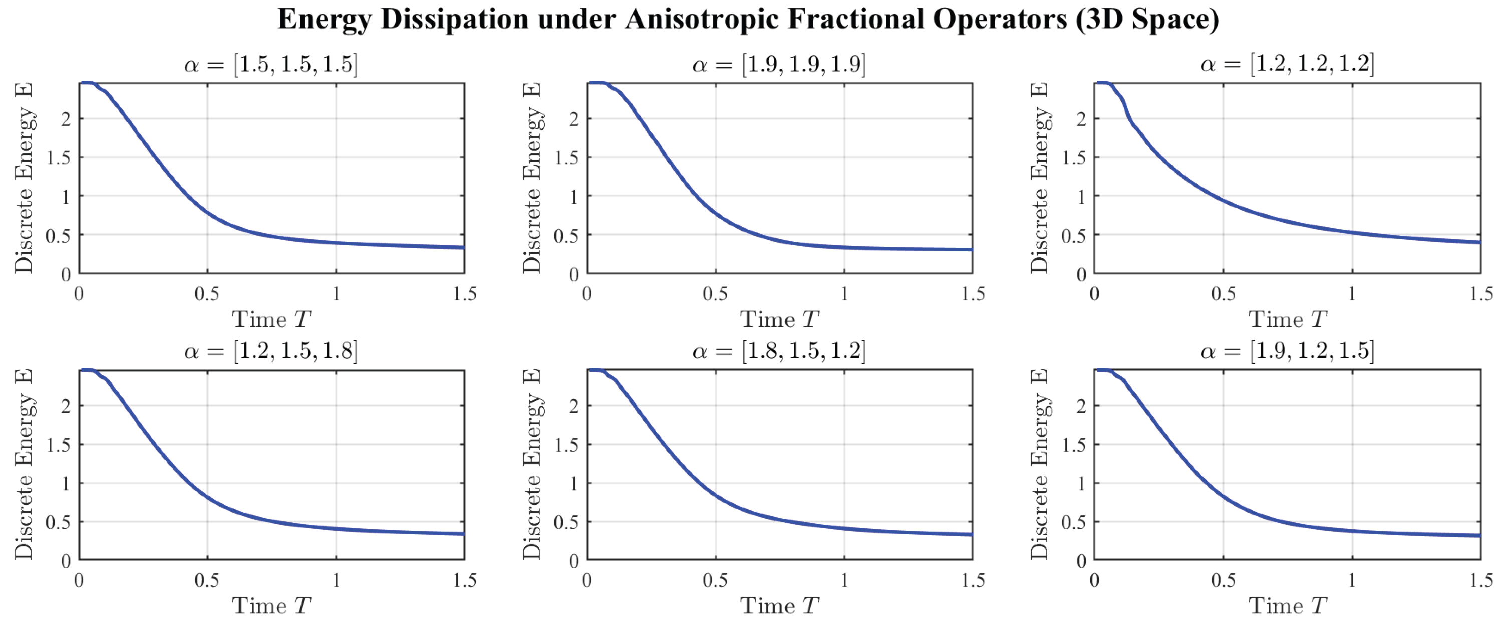
Figure 2.
3D phase separation morphologies under different combinations of anisotropic fractional orders.
Figure 2.
3D phase separation morphologies under different combinations of anisotropic fractional orders.
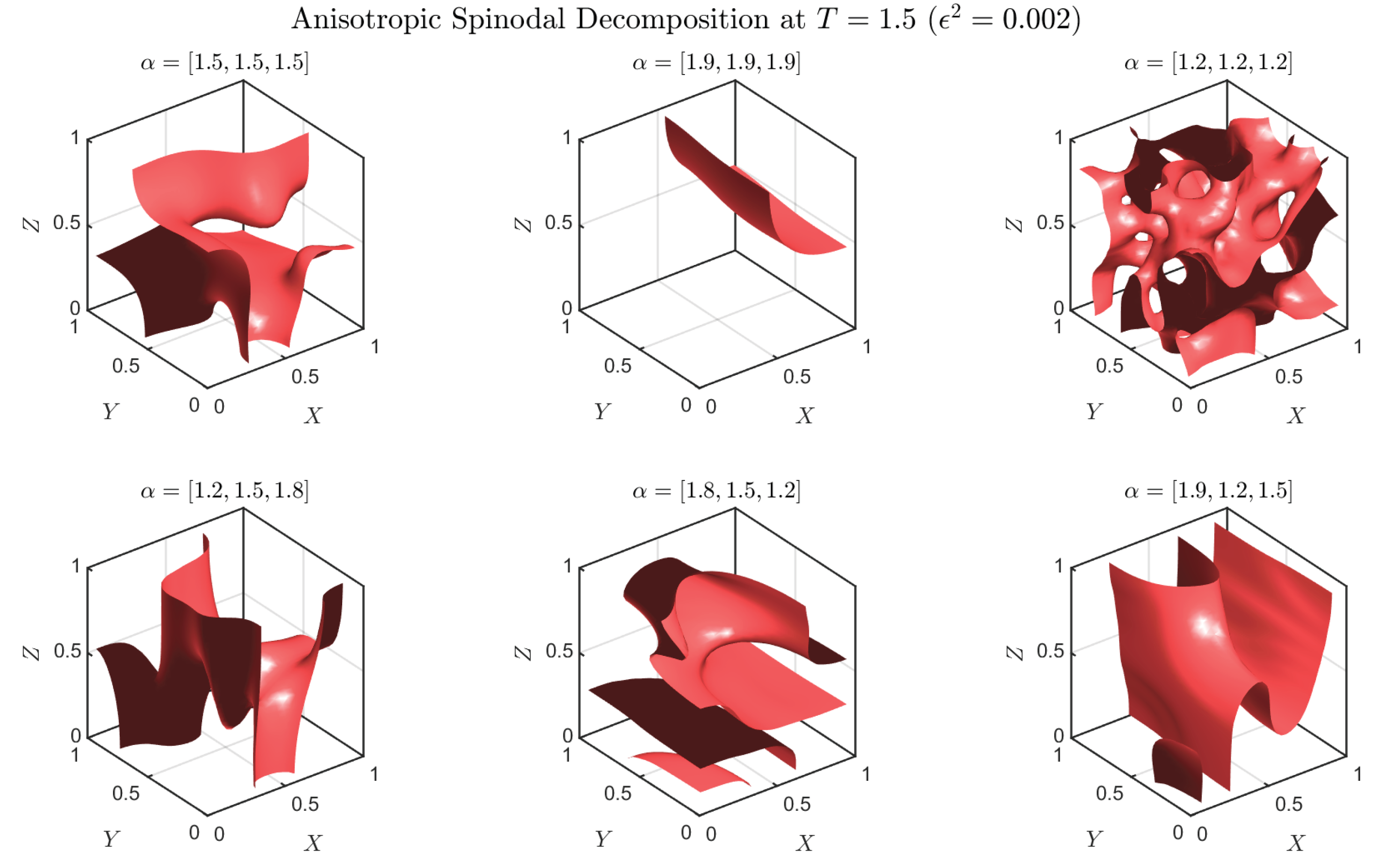
Figure 3.
Execution time scaling of VTP versus Standard DST in high-dimensional spaces (6D to 8D).
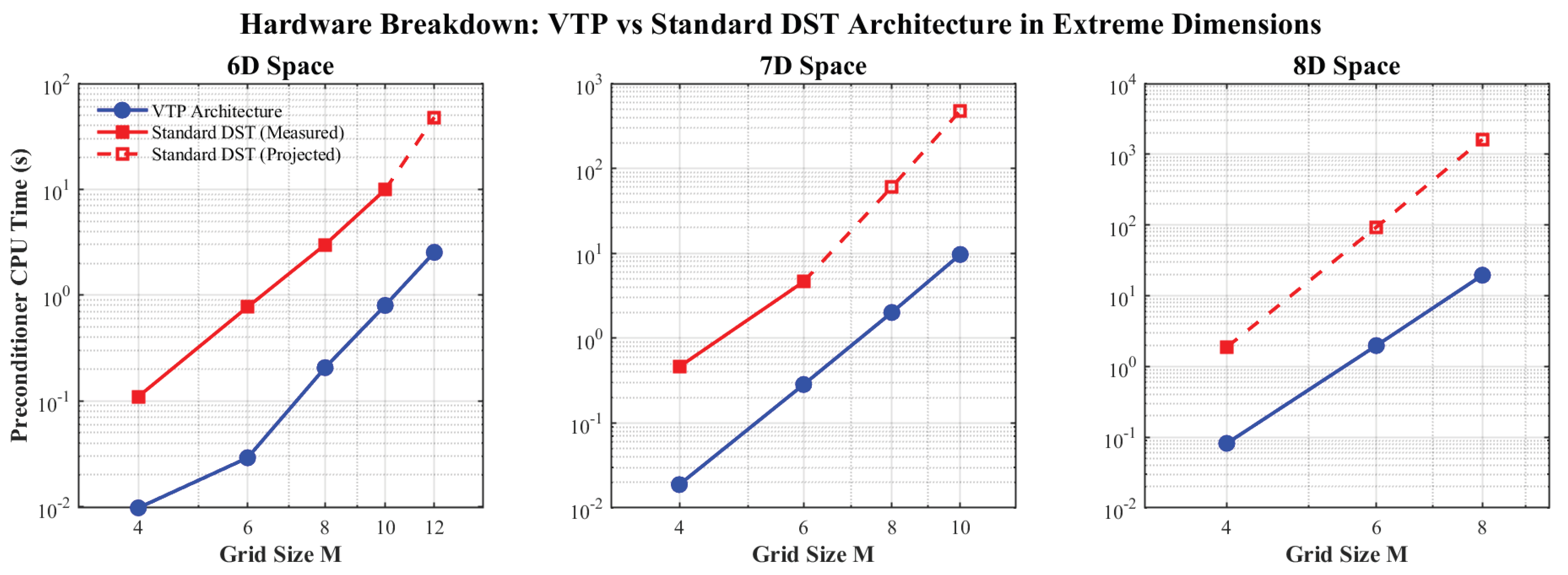
Figure 4.
Total execution time scaling of the proposed framework versus the baseline in high-dimensional spaces (6D to 8D).
Figure 4.
Total execution time scaling of the proposed framework versus the baseline in high-dimensional spaces (6D to 8D).
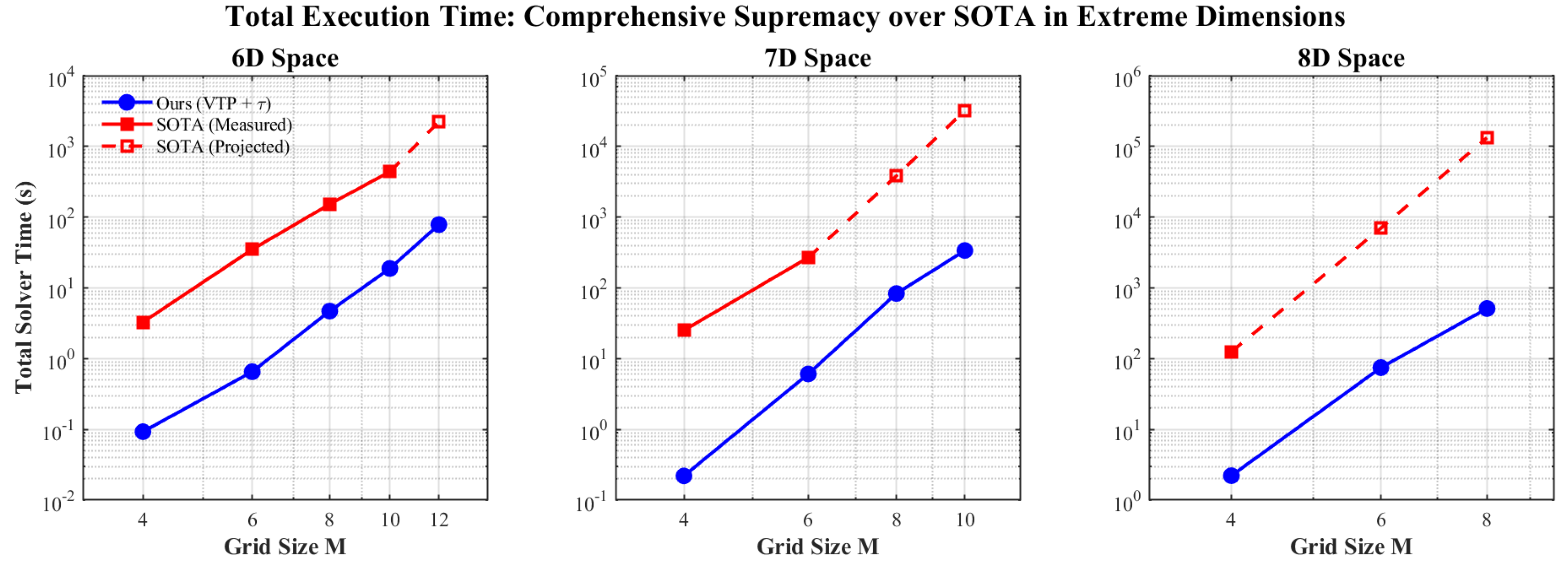
Table 2.
Comparison of single-step execution time between the proposed VTP architecture and Standard DST across varying dimensions and grid resolutions.
Table 2.
Comparison of single-step execution time between the proposed VTP architecture and Standard DST across varying dimensions and grid resolutions.
| Dim | M | DOF (N) | Config () | Execution Time (s) | Speedup | |
|---|---|---|---|---|---|---|
| VTP (Ours) | Std DST | |||||
| 3D | 64 | 262,144 | 0.09655 | 0.20587 | 2.49× | |
| 0.08341 | 0.19902 | 2.50× | ||||
| 0.11064 | 0.20457 | 1.98× | ||||
| 0.10106 | 0.20584 | 2.38× | ||||
| 0.09071 | 0.20621 | 2.39× | ||||
| 0.09288 | 0.20447 | 2.67× | ||||
| 4D | 8 | 4,096 | 0.00320 | 0.02846 | 9.70× | |
| 0.00128 | 0.02693 | 18.17× | ||||
| 0.00124 | 0.02667 | 17.52× | ||||
| 0.00126 | 0.02683 | 27.24× | ||||
| 0.00156 | 0.02818 | 19.80× | ||||
| 0.00140 | 0.02756 | 16.80× | ||||
| 12 | 20,736 | 0.00325 | 0.09221 | 27.40× | ||
| 0.00287 | 0.09282 | 34.87× | ||||
| 0.00265 | 0.09280 | 29.05× | ||||
| 0.00388 | 0.09403 | 41.60× | ||||
| 0.00321 | 0.09554 | 27.58× | ||||
| 0.00291 | 0.09478 | 30.88× | ||||
| 5D | 4 | 1,024 | 0.00139 | 0.01770 | 10.81× | |
| 0.00046 | 0.01627 | 32.75× | ||||
| 0.00045 | 0.01624 | 29.67× | ||||
| 0.00049 | 0.01620 | 27.41× | ||||
| 0.00056 | 0.01610 | 29.46× | ||||
| 0.00046 | 0.01632 | 35.55× | ||||
| 6 | 7,776 | 0.00277 | 0.08569 | 21.85× | ||
| 0.00310 | 0.08228 | 36.59× | ||||
| 0.00291 | 0.08384 | 30.36× | ||||
| 0.00280 | 0.08299 | 26.70× | ||||
| 0.00260 | 0.08239 | 26.22× | ||||
| 0.00310 | 0.08266 | 26.57× | ||||
| 8 | 32,768 | 0.01547 | 0.27134 | 25.20× | ||
| 0.01407 | 0.26958 | 14.27× | ||||
| 0.01459 | 0.26590 | 18.77× | ||||
| 0.01556 | 0.27062 | 16.95× | ||||
| 0.01621 | 0.27003 | 18.21× | ||||
| 0.01491 | 0.27305 | 21.89× | ||||
Table 3.
Comparison of total solver time between the complete -preconditioned VTP framework and the representative baseline algorithm.
Table 3.
Comparison of total solver time between the complete -preconditioned VTP framework and the representative baseline algorithm.
| Dim | M | DOF (N) | Config () | Iterations | Total Solver Time (s) | Speedup | ||
|---|---|---|---|---|---|---|---|---|
| VTP (Ours) | Baseline | VTP (Ours) | Baseline | |||||
| 3D | 64 | 262,144 | 15 | 39 | 2.2299 | 11.5844 | 4.9× | |
| 15 | 39 | 1.7862 | 11.3915 | 5.1× | ||||
| 15 | 39 | 1.6038 | 11.8063 | 5.5× | ||||
| 15 | 39 | 1.7222 | 11.2300 | 6.0× | ||||
| 15 | 39 | 1.7646 | 11.3986 | 6.2× | ||||
| 15 | 39 | 1.8994 | 11.6291 | 7.6× | ||||
| 4D | 8 | 4,096 | 15 | 26 | 0.0635 | 1.0997 | 20.2× | |
| 15 | 26 | 0.0374 | 1.0518 | 24.3× | ||||
| 15 | 26 | 0.0272 | 1.0247 | 28.1× | ||||
| 15 | 26 | 0.0334 | 1.0179 | 33.6× | ||||
| 15 | 26 | 0.0258 | 1.0154 | 32.9× | ||||
| 15 | 26 | 0.0271 | 1.0187 | 34.8× | ||||
| 12 | 20,736 | 15 | 29 | 0.0882 | 3.9049 | 72.0× | ||
| 15 | 29 | 0.0585 | 3.9537 | 65.4× | ||||
| 15 | 29 | 0.0657 | 3.9907 | 59.5× | ||||
| 15 | 29 | 0.0702 | 4.0046 | 73.2× | ||||
| 15 | 29 | 0.0646 | 4.0071 | 55.0× | ||||
| 15 | 29 | 0.0641 | 4.0268 | 62.8× | ||||
| 5D | 4 | 1,024 | 15 | 25 | 0.0407 | 0.9306 | 15.0× | |
| 15 | 25 | 0.0107 | 0.6252 | 52.0× | ||||
| 15 | 25 | 0.0101 | 0.6055 | 46.5× | ||||
| 15 | 25 | 0.0101 | 0.6113 | 48.4× | ||||
| 15 | 25 | 0.0104 | 0.6042 | 61.1× | ||||
| 15 | 25 | 0.0098 | 0.6171 | 57.2× | ||||
| 6 | 7,776 | 15 | 27 | 0.0966 | 3.4978 | 59.5× | ||
| 15 | 27 | 0.0871 | 4.1575 | 57.2× | ||||
| 15 | 27 | 0.0893 | 4.1048 | 37.7× | ||||
| 15 | 27 | 0.0970 | 4.0479 | 63.2× | ||||
| 15 | 27 | 0.0870 | 3.9684 | 43.0× | ||||
| 15 | 27 | 0.0808 | 3.5902 | 40.7× | ||||
| 8 | 32,768 | 15 | 29 | 0.4051 | 16.1457 | 28.9× | ||
| 15 | 29 | 0.3822 | 13.6345 | 36.0× | ||||
| 15 | 29 | 0.3928 | 12.6956 | 37.0× | ||||
| 15 | 29 | 0.4054 | 13.1391 | 53.2× | ||||
| 15 | 29 | 0.3748 | 11.9373 | 40.2× | ||||
| 15 | 29 | 0.3796 | 13.9693 | 43.2× | ||||
Disclaimer/Publisher’s Note: The statements, opinions and data contained in all publications are solely those of the individual author(s) and contributor(s) and not of MDPI and/or the editor(s). MDPI and/or the editor(s) disclaim responsibility for any injury to people or property resulting from any ideas, methods, instructions or products referred to in the content. |
© 2026 by the authors. Licensee MDPI, Basel, Switzerland. This article is an open access article distributed under the terms and conditions of the Creative Commons Attribution (CC BY) license (http://creativecommons.org/licenses/by/4.0/).
Copyright: This open access article is published under a Creative Commons CC BY 4.0 license, which permit the free download, distribution, and reuse, provided that the author and preprint are cited in any reuse.


