

Submitted:
20 April 2026
Posted:
21 April 2026
You are already at the latest version
Abstract
Manual review of ambulatory EEG (aEEG) for epilepsy monitoring is time-consuming, challenging due to artifacts, and prone to human error. To address this, we developed a machine learning-based automated seizure detection system. We collected 3140 hours of aEEG recordings from 48 patients, including 15 with documented seizures (88 total events). Data was preprocessed, segmented into 5-second overlapping epochs, and extracted for time and frequency domain features. A channel-wise ensemble approach combining XGBoost, CatBoost, and LightGBM was trained on 70% of the data and evaluated using 10-fold cross-validation. The model achieved high accuracy (98.4% ± 1.3%) and specificity (98.4% ± 1.3%) during training. Testing confirmed robust performance with 99.64% ± 1.3% accuracy and 99.78% ± 0.62% specificity. The average AUC was 0.94, and the false detection rate was minimal at 0.43 events per hour. The proposed ensemble machine learning framework reliably identifies seizures from aEEG data, achieving high accuracy while keeping false detections significantly low.
Keywords:
machine learning
; statistical analysis
; seizure detection
; ensemble technique
; signal processing
; ambulatory EEG
1. Introduction
Epilepsy is a chronic neurological condition often characterized by recurrent and unprovoked seizures, affecting 65 million people worldwide [1]. The electroencephalogram (EEG) remains the primary clinical tool for both diagnostic and seizure monitoring. However, a significant clinical challenge arises from the sporadic and unpredictable nature of seizures, which makes capturing these events during brief clinical recordings difficult. The primary diagnostic modalities, outpatient EEG and admission to the Epilepsy Monitoring Unit (EMU), present distinct limitations. The routine outpatient EEG, typically lasting 20-40 minutes, provides increased accessibility but suffers from low diagnostic yield for seizure and interictal discharges (sensitivity: 32–59%) [2,3]. In contrast, the EMU admission provides a ‘gold standard’ for seizure characterization through continuous, long-term monitoring, but it is resource-intensive, costly, and requires a protracted hospital stay.
For patients who need to complete a diagnostic evaluation, the ambulatory EEG (aEEG) offers a cost-effective, non-invasive alternative to capture epileptic activities with higher sensitivity (72%), allowing patients to record their EEG at home [2,4]. The clinical utility of aEEG is undoubtedly useful, as long-term recordings spanning several days to weeks increase the chances of capturing infrequent seizures [5]. However, the current process of manual EEG evaluation can be time-consuming due to the extensive duration of EEG recordings. The limited and inefficient automated seizure detection systems for aEEG underscore the need for such tools that can assist clinicians in efficiently reviewing long-term aEEG recordings.
aEEG can be challenging due to the numerous artifacts present in the EEG. There are a few clinically approved tools such as ENCEVIS (sensitivity: 77.8%, False Positives per Hour [FP/Hr.]: 0.2), Besa (sensitivity: 67.6%, FP/Hr.: 0.7) and PERSYST (sensitivity: 81.6%, FP/Hr.: 0.9) that are being adopted for seizure detection in aEEG, but their effectiveness in seizure detection is limited [6]. On the other hand, several such algorithms are available for routine and EMU EEG in research that can detect seizures based on statistical or machine learning approaches, such as Support Vector Machine (SVM), K-Nearest Neighbor (k-NN), Artificial Neural Network (ANN), and Linear Discriminant Analysis (LDA) [7]. Additionally, several boosting techniques have also been proven to be effective in seizure detection. Previous reports suggest XGBoost (Accuracy: 88-94.3%) [8,9], CatBoost (Accuracy: 95.7%) [10] and RUSBoost (Accuracy: 93.4%) [11] have performed superiorly in detecting seizures using multiple EEG and MEG datasets. The above studies frequently used the publicly available CHB-MIT dataset [12], the BONN University EEG dataset [13] or the TUH EEG Corpus [14]. While these datasets are highly reliable, they have been curated to contain reduced noise and artifacts, which makes them less suitable for real-world applications. It is also challenging to achieve the same level of detection accuracy, sensitivity, and specificity with unseen new patient data. We need a more robust algorithmic approach that can analyze unprocessed EEG data to produce accurate seizure detection with high specificity and sensitivity while maintaining a low false detection rate for aEEG.
In the proposed study, we developed an efficient and accurate seizure detection pipeline that calculates a set of defined features from aEEG data, implements data normalization, uses an ensembled machine learning approach (XGBoost, CatBoost, and LightGBM algorithms) to detect seizures based on specified confidence thresholds, and post-processes the detections to efficiently consolidate and isolate the entire seizure events. The proposed system can significantly reduce the time required to manually evaluate aEEG while maintaining high sensitivity and low false detection rate, providing a more practical and scalable solution for long-term epilepsy monitoring.
2. Materials and Methods
2.1. Patient Selection Dataset Collection
Forty-eight adult patients (18-80 years old) with suspected epilepsy were randomly selected under a protocol approved by the institutional review board at the University of Illinois Chicago. The patients underwent long-term aEEG monitoring using a 10-20 referential montage system (Neurotech LLC, Wisconsin, USA) with a sampling rate of 200Hz/250Hz or 256 Hz. The EEG files were prefiltered to 0.1Hz- 70Hz during recording. We excluded non-EEG electrodes from the analysis. Two experienced epileptologists independently reviewed and annotated the aEEG recordings for seizures. Further, consensus was reached through mutual discussion, and the final seizure annotations were set as the gold standard. A total of 15 patients experienced at least one seizure, and the remaining 33 patients served as negative controls.
2.2. Data Analysis
The data analysis was performed in multiple steps, including data preprocessing, feature extraction, model selection, and evaluation using Python 3.10 and libraries MNE, NumPy, SciPy, Sklearn, Pandas, XGBoost, CatBoost, and LightGBM. A high-level layout of the data analysis pipeline is outlined in Figure 1.
Data preparation: The aEEG for each patient was imported along with the corresponding gold standard annotations. Data files with a sampling rate higher than 200Hz were resampled to 200Hz to maintain consistency in data processing and feature extraction. Further, the data was filtered using a 1-40Hz zero-phase fourth-order Butterworth bandpass digital filter that captured 91.18% of the power content in the signal while eliminating any excessive information from other frequencies. The data set contained ocular, myogenic, and extrinsic types of noise, which potentially could impact the parameters used for seizure detection. We implemented wavelet transformation using Daubechies (db4) and mean absolute difference (MAD) on our dataset for noise reduction because of its better performance and low time complexity [7,15,16,17]. After extracting wavelet coefficients, we remove anomalous coefficient which has a large median absolute difference. This way, the slow waves get reduced, and noisy segments get smoothed.
Feature extraction and engineering: The denoised signal was used for feature extraction and engineering to evaluate the best features that separate the seizures from the rest of the signal. The EEG signal in each file contained 19 channels. This channel data was divided into 5-second sliding windows with a 50% overlap. For each data window, for each channel, we extracted 11-time domain (mean, standard deviation, kurtosis, line length, log of total signal power, Hjorth’s complexity and mobility, signal power, average peak to peak count, fractal dimension, zero crossing) and 5 frequency domain features (Delta (1-3Hz) power, Theta (4-7) power, Alpha (8-12) power, Beta (13-30) power, low Gamma (30-40) power) [18,19,20]. These features were selected based on their low time complexity to process an EEG file.
The data in the feature space were scaled differently depending on the patient’s EEG, which needed normalization. We applied z-score normalization to each feature within each channel in a file, ensuring the data was normally distributed, comparable across files, and suitable for machine learning. The extracted feature data was tagged with the gold standard seizure annotations for evaluation. Following normalization, we curated a balanced dataset for model training and evaluation by including all feature values corresponding to seizure data and randomly selecting one hour of non-seizure feature data from each aEEG file collected per patient. We implemented t-distributed stochastic neighbor embedding (t-SNE) to reduce dimension and visualize the separability of these features between seizure and non-seizure data.
2.3. Machine Learning Models
We used XGBoost [21], CatBoost [22], LightGBM [23], Balanced Random Forest (BRF) [24], and RUSBoost [25] models to train on our data. To optimize the performance of these algorithms, Randomized Grid Search was employed for efficient hyperparameter tuning, ensuring that each model achieves robust performance for the training and validation datasets. These algorithms were selected for their proven effectiveness in handling the complexities of seizure detection and imbalanced datasets. Each channel’s data was used to train a separate model for each algorithm, resulting in a total of 95 models (19 channels × 5 algorithms). The feature importance for each model was evaluated to understand the contribution of individual features within each algorithmic approach. To enhance predictive accuracy and robustness, we ensembled the top three models (based on their performance metrics across all channels) using a voting method. In this approach, each model votes for its predicted class, and the majority or weighted consensus serves as the final output, curbing individual bias and variance, limiting overfitting and channel-specific bias, and yielding stable, accurate binary-classification results.
2.4. Model Validation
We divided the dataset into a 70% training set and a 30% testing set. A 10-fold cross-validation method was implemented to validate the algorithm’s performance during training. Test time evaluation was performed by calculating accuracy, sensitivity (true positive rate), specificity (true negative rate), and ROC-AUC. Data shuffling was applied to randomize the dataset, preventing the model from learning unintended patterns based on sequential data order, thereby enhancing its generalization ability. The combined approach of data shuffling, data splitting, and multi-fold cross-validation ensured a thorough and reliable validation of the model’s predictive capabilities.
2.5. Post Processing
Once the model prediction was done, we used post-processing to consolidate the individual segments of a seizure into a single event per seizure. We first established a prediction confidence threshold for each channel-wise model (as shown in Figure 5c) and combined the prediction results for each EEG segment using an ensemble approach across channels. This ensemble employed a voting mechanism, where the class with the maximum votes was selected as the final predicted class. Once final predictions were obtained for each EEG segment across all channels, a consolidation process was implemented. Specifically, if at least 12 channels within a corresponding time segment were marked as seizure, that time segment was classified as a seizure segment. Consecutive seizure segments were further consolidated into a single seizure event to ensure temporal continuity. Finally, the consolidated results were converted back into the EDF annotation format and provided to the end user for an additional round of verification, ensuring accuracy and reliability in the final output.
3. Results
We have developed a seizure detection algorithm for aEEG using a retrospective dataset from 48 patients who underwent long-term aEEG monitoring. The study evaluated a range of temporal and spectral features along with normalization techniques to quantitatively characterize features in discriminating seizure and non-seizure EEG segments. Subsequently, we developed channel-wise XGBoost, CatBoost, LightGBM, BRF, and RUSBoost models to evaluate the efficacy of the extracted features in identifying the seizures. The refined and normalized features and selected models were integrated into a pipeline to classify windowed aEEG data to seizure or non-seizure events. Finally, the model output was consolidated to generate annotations for validation and the seizure markings on EEG files.
3.1. Feature Evaluation
We evaluated 11-time domain (mean, standard deviation, kurtosis, line length, log signal power, Hjorth’s complexity and mobility, signal power, average peak to peak count, fractal dimension, zero crossing) and 5 frequency domain (Delta (1-3Hz) power, Theta (4-7) power, Alpha (8-12) power, Beta (13-30) power, low Gamma (30-40) power) features to find the features that would significantly differentiate the seizure from non-seizure EEG in each electrode (Figure 2). To evaluate the significance and contribution of features in our seizure detection model, we conducted a comprehensive feature study using P-value analysis between seizure and non-seizure data, correlation analysis to evaluate the relationship between features, SHAP (SHapley Additive exPlanations) analysis to rank the features based on their contribution to the results of different machine learning models and t-distributed Stochastic Neighbor Embedding (t-SNE) to understand separation of training data between classes.
We scaled the features to compare the feature value differences between seizure and non-seizure segments. All frequency-based features were scaled by 1e14 prior to calculation. Most features were multiple fold higher in seizure segments as compared to non-seizure segments. Among the extracted features, Gamma (fold: 605.95 ± 1886.47), Beta (321.76 ± 1065.29), Alpha (48.81 ± 147.17), Theta (11.57 ± 15.56), Delta (9.10 ± 10.73), total Power (10.84 ± 12.50), Peak Count (10.54 ± 6.60), Line Length (4.06 ± 3.82), Standard Deviation (2.84 ± 1.61), Mean (1.20 ± 0.47), Mobility (1.41 ± 0.63), and Zero Crossings (1.29 ± 0.52) were significantly (p<0.05) elevated by multiple folds in seizure segments when compared with non-seizure segments. Fractal Dimension (0.94 ± 0.04) and Complexity (0.94 ± 0.17) were reduced during seizures, while Energy (1.08 ± 0.13) and Kurtosis (1.02 ± 0.91) showed minimal differences independently between event types. Out of 304 feature tests (16 features across 19 channels), 302 were found to be significantly differentiating seizure vs non-seizure segments (P < 0.05, Mann-Whitney U test). Kurtosis on Channel Fp2 (p = 0.304) and F4 (p =0.099) didn’t meet the desired significance.
3.1.1. Inter-Feature Correlation Analysis
Inter-feature correlation analysis (Figure 3a,b) revealed distinct coupling patterns between seizure and non-seizure states. In the non-seizure state, strong positive correlations (r > 0.9) were observed among Kurtosis–Std, Line-length–Gamma, and Mobility–Zero-crossings, whereas spectral bands (Alpha, Beta, Delta, Gamma) showed moderate correlation (r > 0.7). Feature pairs Mobility–Energy (r ≈ –0.91) and Zero crossings–Theta (r ≈ –0.99) demonstrated anti-correlation reflecting reduced complexity with increased rhythmicity. During seizures, spectral and amplitude-based features became more tightly coupled (r > 0.9), and anti-correlation relationships involving Mobility, Theta, and Zero-crossings strengthened further.
The correlation dynamics reveal large shifts between seizure and non-seizure states, with differences exceeding a correlation delta (Δ) of 0.40. Normalization further amplified these differences. Before normalization (Figure 3A), the Energy–Fractional Dimension pair showed a negative shift (Δ ≈ –0.35), the Std–Energy pair exhibited a moderate negative difference (Δ ≈ –0.30), and the Line Length–Mobility pair showed a mild positive shift (Δ ≈ +0.25). After normalization (Figure 3B), these contrasts became more pronounced, with Energy–Fractional Dimension decreasing further (Δ ≈ –0.45), Std–Energy reaching Δ ≈ –0.45, and Line Length–Mobility increasing to Δ ≈ +0.45, indicating enhanced separation between seizure and non-seizure feature correlations following normalization.
Further, we performed t-SNE dimensionality reduction on the training dataset and investigated the data separability (Figure 3C). The resulting t-SNE plot (trustworthiness score: 97.38%) suggests that while the seizure and non-seizure data are not entirely separable, distinct clusters can still be observed, indicating that with sufficient training, the model can learn to distinguish seizure segments from non-seizure segments effectively.
Upon thorough understanding of the feature space, we further evaluated how these individual features contribute toward the decision boundaries within each model (Figure 4). While there is variability in SHAP rankings across models, a consistent pattern emerged; features like Complexity, Line Length, Gamma, and Kurtosis remained among the top contributors across XGBoost, LightGBM, and CatBoost. In XGBoost and LightGBM, these features achieved mean SHAP ranks of approximately 13 ± 1.2 and 15 ± 0.8, respectively, reflecting strong discriminative influence across both temporal and spectral domains, with CatBoost exhibiting comparable trends. Using an elbow criterion on the mean SHAP distributions, a natural cutoff appeared around the top 5–6 features, beyond which cumulative importance plateaued (< 5% change). When SHAP indices were averaged across all models, the most stable predictors of seizure classification included Complexity, Line Length, Gamma, Kurtosis, Beta, and Mean, indicating that nonlinear dynamics, waveform irregularity, and spectral composition collectively drive the most significant model decisions.
3.2. Model Development and Performance Evaluation
We implemented five machine learning models, namely XGBoost (XGB), CatBoost (CB), LightGBM (LGBM), RUSBoost (RUSB), and Balanced Random Forest (BRF) and further constructed an ensemble model (ESBL) from the top-performing classifiers. Model performance was assessed based on accuracy, sensitivity, specificity, ROC-AUC, and false positives per hours (FP/Hr.), across both training and testing datasets (Table 1).
3.2.1. Individual Model Performance
XGBoost (XGB) consistently outperformed other models, achieving 98.76% accuracy with an AUC score of 0.92 on the test dataset. However, its sensitivity on the test set was 54.80%, suggesting some limitations in detecting seizure events despite its high specificity (99.32%) (Table 1). CatBoost (CB) and LightGBM (LGBM) also demonstrated strong performance with 96.48% and 97.93% accuracy on the test set, respectively. Notably, CatBoost exhibited the highest sensitivity among the top three models (68.29%), making it particularly useful for seizure event detection. However, it had a relatively higher false positive rate (FP/Hr. = 0.6) compared to XGBoost (0.34 FP/Hr.). LightGBM balanced performance well, achieving 62.87% sensitivity and a lower false positive rate (0.47 FP/Hr.) than CatBoost (Table 1).
In contrast, RUSBoost and Balanced Random Forest exhibited considerable limitations in seizure detection. RUSBoost showed the lowest sensitivity (41.00% on the test set) and the lowest ROC-AUC score (0.84), suggesting poor seizure event discrimination. Balanced Random Forest (BRF) performed better than RUSBoost but still lagged behind XGB, CB, and LGBM, with a test sensitivity of 74.45% and a moderate ROC-AUC of 0.89.
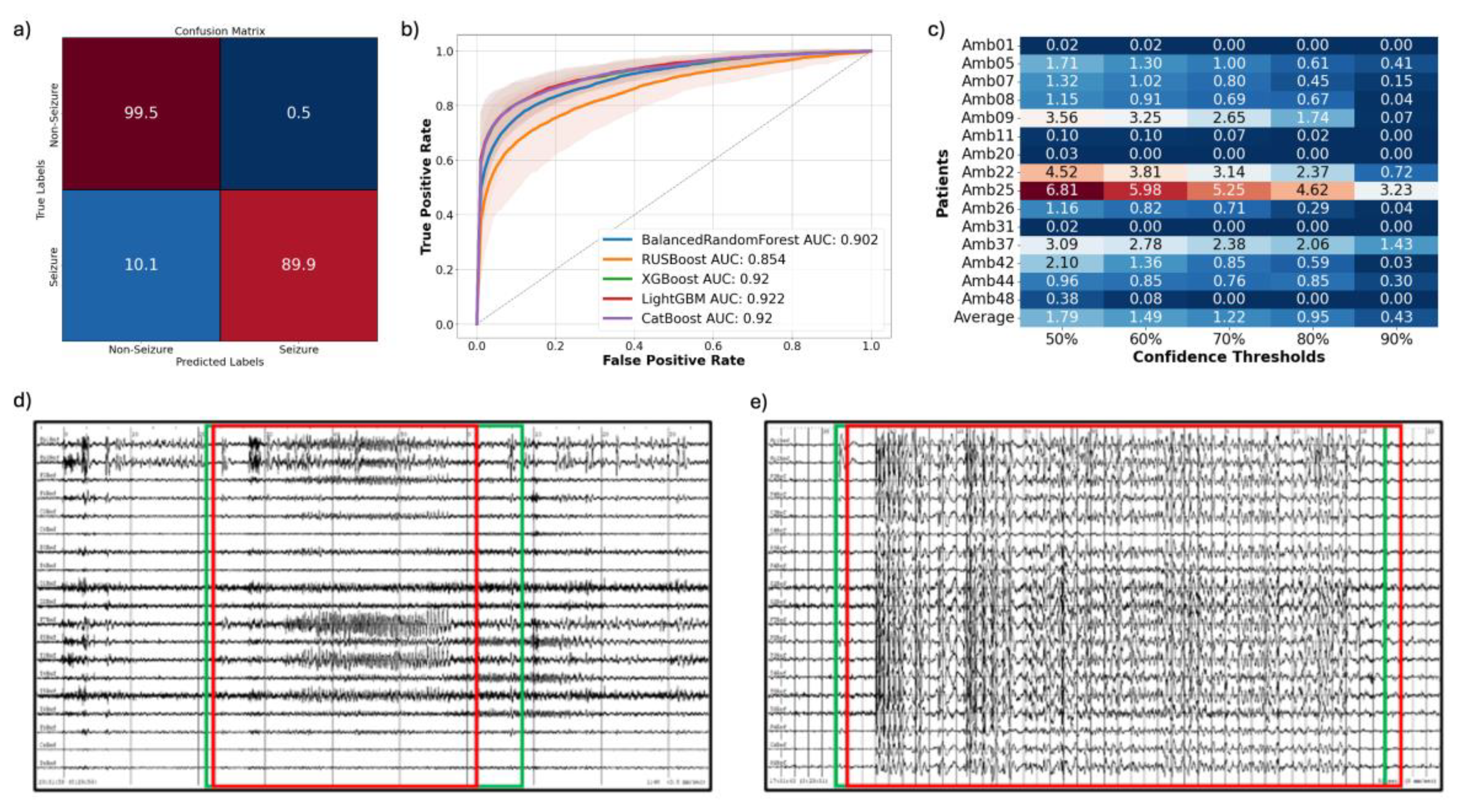
Figure 5.
Overview of results. (a) Confusion matrix showing the final classification performance in percentages after applying post-processing techniques. (b) ROC AUC curve for the Machine Learning Models. (c) False positives per hour plotted for individual patient files against varying confidence thresholds, illustrating the impact of threshold selection on model performance. (d,e) Final seizure annotations after post-processing on an EDF file. Red box denotes doctors’ annotation while the green box denotes our model annotations.
Figure 5.
Overview of results. (a) Confusion matrix showing the final classification performance in percentages after applying post-processing techniques. (b) ROC AUC curve for the Machine Learning Models. (c) False positives per hour plotted for individual patient files against varying confidence thresholds, illustrating the impact of threshold selection on model performance. (d,e) Final seizure annotations after post-processing on an EDF file. Red box denotes doctors’ annotation while the green box denotes our model annotations.
3.2.2. Ensemble Model Performance
Based on a comparative evaluation of multiple classifiers (Table 1), XGBoost, CatBoost, and LightGBM emerged as the top performers, each providing balanced accuracy, sensitivity, and specificity. To harness their complementary strengths, we constructed an ensemble model using a majority-voting strategy, in which the final classification was determined by the consensus of the three models. This approach yielded a marked improvement over individual classifiers, achieving an overall accuracy of 99.64%, sensitivity of 89.00%, and specificity of 99.64%, with a false positive rate of 0.427 FP/Hr. on the test dataset. These results demonstrate that ensemble learning provides superior stability and reliability in seizure detection compared with single-model approaches.
3.2.3. Post Processing Results
To further enhance predictive reliability, we implemented an adaptive probability thresholding strategy, replacing the default 50% cutoff with dynamic thresholds ranging from 50% to 90%. By requiring higher confidence for classifying seizure events, this approach effectively reduced false positives while preserving overall accuracy. For instance, at a 60% threshold, a probability distribution of [0.38, 0.62] was classified as seizure, whereas [0.43, 0.57] was classified as non-seizure, thereby filtering out low-confidence predictions. As shown in Figure 5c, increasing the confidence threshold led to a marked reduction in false-positive rates. For example, in patient Amb25, false positives decreased from 6.91 to 3.23 per hour, while overall accuracy improved from 96.84% to 99.1%. Setting the confidence threshold at 90% eliminated most ambiguous predictions, providing more stable and trustworthy seizure detection performance.
In addition to probability refinement, we applied post-processing at the channel level. A minimum threshold of 12 channels was established, such that at least 12 models per channel are needed to indicate seizure activity for an event to be classified as a seizure. This constraint suppressed spurious detections from isolated channels and further minimized edge-case misclassifications.
The effect of this dual thresholding strategy is illustrated in Figure 5, where reductions in false positives per hour across patients are shown in panel (c). The corresponding impact on classification reliability is summarized in the confusion matrix (Figure 5a), while panels (d) and (e) display the alignment of final predicted seizure segments with EDF ground-truth annotations. Together, these results confirm that probabilistic and channel-level thresholding significantly improve seizure detection specificity without compromising sensitivity.
4. Discussion
We developed and validated a robust seizure detection pipeline for ambulatory EEG (aEEG), integrating optimized feature engineering, an ensemble of gradient-boosting models (XGBoost, CatBoost, and LightGBM), and targeted post-processing. On a 48-patient retrospective dataset, this approach achieved high sensitivity (89.00%) and a low false positive rate (0.427 events/hr.).
A primary challenge in aEEG is mitigating noise artifacts without compromising computational efficiency. We determined that a db4 wavelet transform combined with Median Absolute Deviation (MAD) filtering provided the optimal tradeoff. This preprocessing was essential for stabilizing the 302 (of 304) temporal and spectral features we identified as statistically significant (e.g., Mobility, Line Length). Our feature analysis also underscored the need for practical validation; features like sample entropy were excluded due to high computational cost, while Kurtosis and Complexity were rejected for producing unreliable NaN outputs, despite their theoretical relevance.
The dataset’s severe class imbalance rendered standard resampling techniques like RUSBoost ineffective, likely due to the loss of rare seizure-specific information. Gradient boosting models performed better individually but offered a clear tradeoff between sensitivity (CatBoost) and specificity (XGBoost). Our majority-vote ensemble successfully leveraged these complementary strengths to achieve a superior, balanced performance that outperformed any single classifier.
To further refine predictions, we implemented a 0.6 probability threshold and a 12-channel consensus requirement. This post-processing was critical for managing the class imbalance, effectively filtering low-confidence, likely false-positive detections and spurious, localized noise events.
Clinically, our algorithm’s 89% sensitivity significantly exceeds that of deployed tools such as Persyst (81.6%), Besa (67.6%), and Encevis (77.8%), while maintaining a competitive false positive rate (0.427 FP/Hr.) [6]. This superior sensitivity presents a critical advantage for ambulatory monitoring, where minimizing missed seizures is paramount. While this ensemble approach is promising, key limitations remain the presence of residual noise artifacts and the inherent class imbalance. Future work should therefore focus on more advanced data augmentation, synthetic sampling, and artifact-handling techniques to improve robustness and generalizability.
Author Contributions
Study concept and design: HH, BM, AS. Data acquisition review and analysis: all authors. Manuscript and figure drafting and preparation: all authors.
Funding
This research was made possible with funding support provided by The Community Health Advocacy Initiative through the University of Illinois Chicago and OSF HealthCare.
Institutional Review Board Statement
The study was conducted in accordance with the Declaration of Helsinki and approved by the Institutional Review Board of the University of Illinois at Chicago (protocol 2022-0492 approved on 6/27/2022).
Conflicts of Interest
The authors declare no conflicts of interest.
References
- J. I. Sirven, “Epilepsy: A Spectrum Disorder,” Cold Spring Harb. Perspect. Med., vol. 5, no. 9, p. a022848, Sep. 2015. [CrossRef]
- L. Hernandez-Ronquillo et al., “Diagnostic Accuracy of Ambulatory EEG vs Routine EEG in Patients With First Single Unprovoked Seizure,” Neurol. Clin. Pract., vol. 13, no. 3, Jun. 2023. [CrossRef]
- W. O. Tatum et al., “Clinical utility of EEG in diagnosing and monitoring epilepsy in adults,” Clinical Neurophysiology, vol. 129, no. 5, pp. 1056–1082, May 2018. [CrossRef]
- U. Seneviratne and W. J. D’Souza, “Ambulatory EEG,” 2019, pp. 161–170. [CrossRef]
- K. A. González Otárula, P. Balaguera, and S. Schuele, “Ambulatory EEG to Classify the Epilepsy Syndrome,” Journal of Clinical Neurophysiology, vol. 38, no. 2, pp. 87–91, Mar. 2021. [CrossRef]
- J. Koren, S. Hafner, M. Feigl, and C. Baumgartner, “Systematic analysis and comparison of commercial seizure-detection software,” Epilepsia, vol. 62, no. 2, pp. 426–438, Feb. 2021. [CrossRef]
- A. A. Ein Shoka, M. M. Dessouky, A. El-Sayed, and E. E.-D. Hemdan, “EEG seizure detection: concepts, techniques, challenges, and future trends,” Multimed. Tools Appl., vol. 82, no. 27, pp. 42021–42051, Nov. 2023. [CrossRef]
- L. Wei and C. Mooney, “Epileptic Seizure Detection in Clinical EEGs Using an XGboost-based Method,” in 2020 IEEE Signal Processing in Medicine and Biology Symposium (SPMB), IEEE, Dec. 2020, pp. 1–6. [CrossRef]
- B. B. R., B. D., C. V., and G. K. R., “Machine Learning-Based Epileptic Seizure Detection Using XGboost Algorithm,” in 2023 International Conference on Recent Advances in Electrical, Electronics, Ubiquitous Communication, and Computational Intelligence (RAEEUCCI), IEEE, Apr. 2023, pp. 1–5. [CrossRef]
- H. Li, “A robust epilepsy diagnosis method based on SDAE and CatBoost,” in 2022 World Automation Congress (WAC), IEEE, Oct. 2022, pp. 46–51. [CrossRef]
- N. Bhanot, N. Mariyappa, H. Anitha, G. K. Bhargava, J. Velmurugan, and S. Sinha, “Seizure detection and epileptogenic zone localisation on heavily skewed MEG data using RUSBoost machine learning technique,” International Journal of Neuroscience, vol. 132, no. 10, pp. 963–974, Oct. 2022. [CrossRef]
- A. L. Goldberger et al., “PhysioBank, PhysioToolkit, and PhysioNet,” Circulation, vol. 101, no. 23, Jun. 2000. [CrossRef]
- R. G. Andrzejak, K. Lehnertz, F. Mormann, C. Rieke, P. David, and C. E. Elger, “Indications of nonlinear deterministic and finite-dimensional structures in time series of brain electrical activity: Dependence on recording region and brain state,” Phys. Rev. E, vol. 64, no. 6, p. 061907, Nov. 2001. [CrossRef]
- A. Harati, S. Lopez, I. Obeid, J. Picone, M. P. Jacobson, and S. Tobochnik, “The TUH EEG CORPUS: A big data resource for automated EEG interpretation,” in 2014 IEEE Signal Processing in Medicine and Biology Symposium (SPMB), IEEE, Dec. 2014, pp. 1–5. [CrossRef]
- G. Inuso, F. la Foresta, N. Mammone, and F. C. Morabito, “Brain Activity Investigation by EEG Processing: Wavelet Analysis, Kurtosis and Renyi’s Entropy for Artifact Detection,” in 2007 International Conference on Information Acquisition, IEEE, Jul. 2007, pp. 195–200. [CrossRef]
- Z. A. A. Alyasseri, A. T. Khader, M. A. Al-Betar, A. K. Abasi, and S. N. Makhadmeh, “EEG Signal Denoising Using Hybridizing Method Between Wavelet Transform with Genetic Algorithm,” 2021, pp. 449–469. [CrossRef]
- Fernando Chamizo, “Denoising with wavelets.” Accessed: Nov. 16, 2024. [Online]. Available: https://matematicas.uam.es/~fernando.chamizo/dark/d_denoisingw.html.
- T. N. Alotaiby, S. A. Alshebeili, T. Alshawi, I. Ahmad, and F. E. Abd El-Samie, “EEG seizure detection and prediction algorithms: a survey,” EURASIP J. Adv. Signal Process., vol. 2014, no. 1, p. 183, Dec. 2014. [CrossRef]
- M. K. Siddiqui, R. Morales-Menendez, X. Huang, and N. Hussain, “A review of epileptic seizure detection using machine learning classifiers,” Brain Inform., vol. 7, no. 1, p. 5, Dec. 2020. [CrossRef]
- Y. Zhang, S. Yang, Y. Liu, Y. Zhang, B. Han, and F. Zhou, “Integration of 24 Feature Types to Accurately Detect and Predict Seizures Using Scalp EEG Signals,” Sensors, vol. 18, no. 5, p. 1372, Apr. 2018. [CrossRef]
- T. Chen and C. Guestrin, “XGBoost,” in Proceedings of the 22nd ACM SIGKDD International Conference on Knowledge Discovery and Data Mining, New York, NY, USA: ACM, Aug. 2016, pp. 785–794. [CrossRef]
- A. V. Dorogush, V. Ershov, and A. Gulin, “CatBoost: gradient boosting with categorical features support,” ArXiv, vol. abs/1810.11363, 2018, [Online]. Available: https://api.semanticscholar.org/CorpusID:26037613.
- G. Ke et al., “LightGBM: A Highly Efficient Gradient Boosting Decision Tree,” in Neural Information Processing Systems, 2017. [Online]. Available: https://api.semanticscholar.org/CorpusID:3815895.
- C. Chen and L. Breiman, “Using Random Forest to Learn Imbalanced Data,” University of California, Berkeley, Nov. 2004.
- C. Seiffert, T. M. Khoshgoftaar, J. Van Hulse, and A. Napolitano, “RUSBoost: Improving classification performance when training data is skewed,” in 2008 19th International Conference on Pattern Recognition, IEEE, Dec. 2008, pp. 1–4. [CrossRef]
Figure 1.
End-to-end EEG seizure detection pipeline. Pipeline illustrating preprocessing, feature engineering, and classification for EEG-based seizure detection. Input EDF files undergo band-pass filtering, wavelet transformation, feature extraction, and global z-normalization. Channel-wise data is processed using XGBoost, LightGBM, and CatBoost, whose outputs are combined through an ensemble model. Final post-processing generates the output annotations distinguishing seizure from non-seizure states.
Figure 1.
End-to-end EEG seizure detection pipeline. Pipeline illustrating preprocessing, feature engineering, and classification for EEG-based seizure detection. Input EDF files undergo band-pass filtering, wavelet transformation, feature extraction, and global z-normalization. Channel-wise data is processed using XGBoost, LightGBM, and CatBoost, whose outputs are combined through an ensemble model. Final post-processing generates the output annotations distinguishing seizure from non-seizure states.
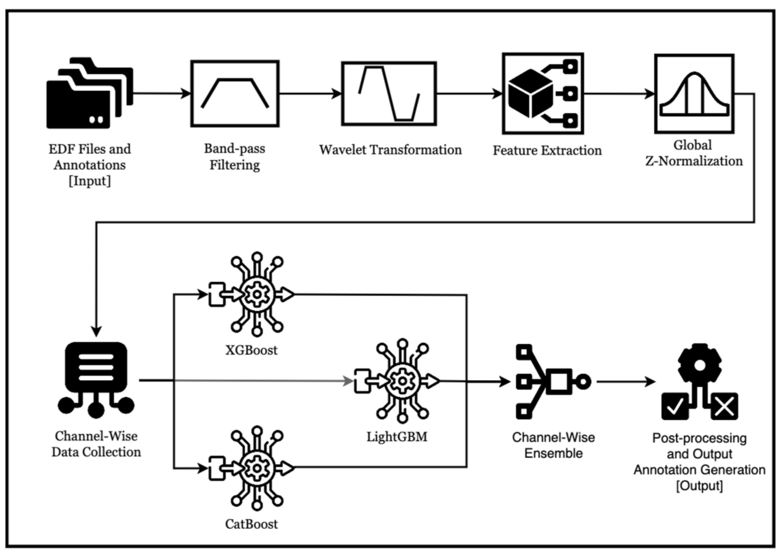
Figure 2.
Feature separation in seizure vs. non-seizure states. Box plots of frequency and time-based EEG features showing distributional differences between seizure and non-seizure segments. The left panel shows features normalized within a single file, while the right panel shows features normalized across all patient files.
Figure 2.
Feature separation in seizure vs. non-seizure states. Box plots of frequency and time-based EEG features showing distributional differences between seizure and non-seizure segments. The left panel shows features normalized within a single file, while the right panel shows features normalized across all patient files.
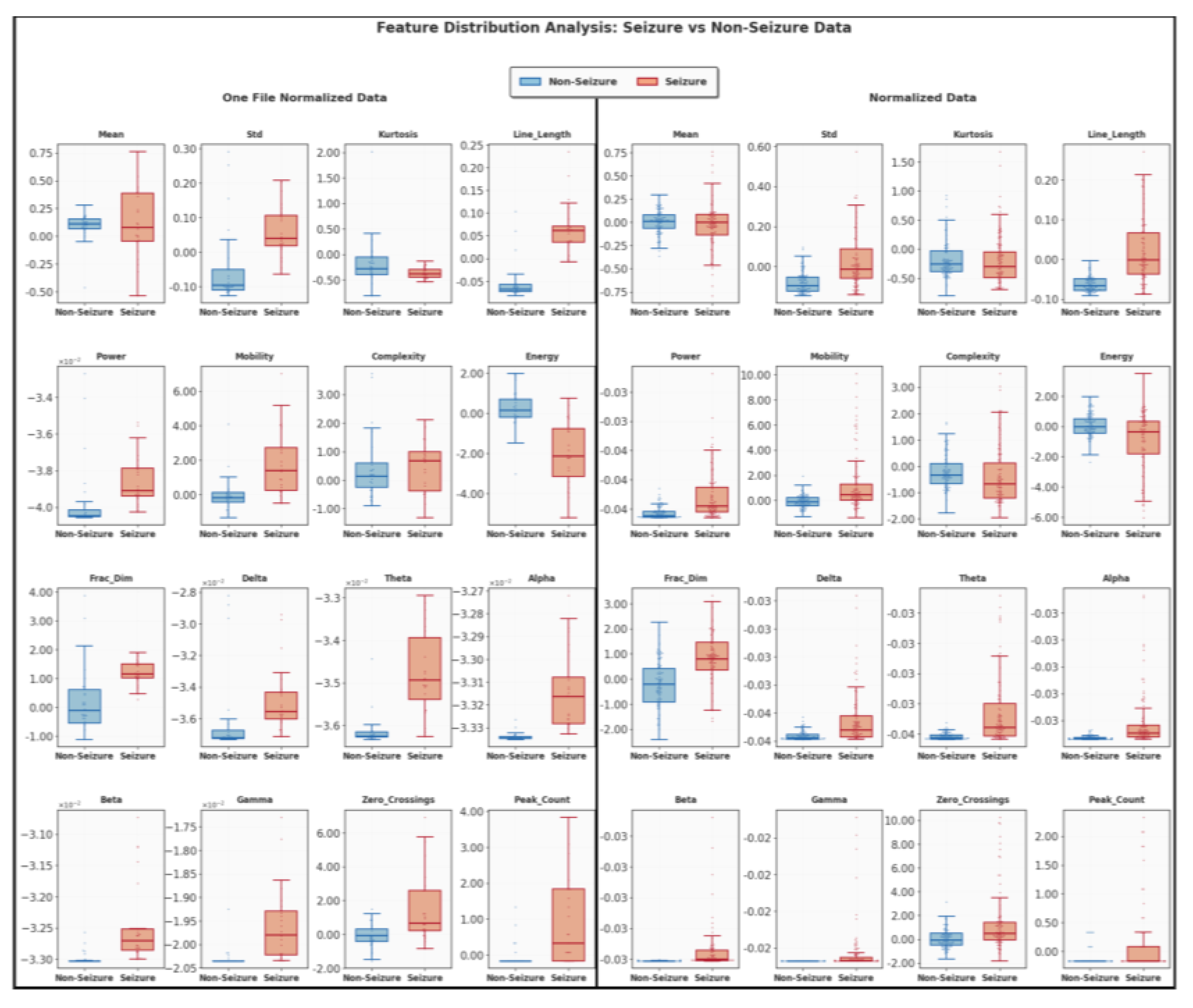
Figure 3.
Inter-feature correlation analysis across seizure and non-seizure data. Correlation matrices comparing EEG feature relationships in seizure and non-seizure states and their difference. (a) correlations from original data without normalization (seizure vs. non-seizure and their difference). (b) same analysis using normalized data, highlighting shifts in inter-feature dependencies between data with and without normalization. (c) t-SNE plots visualizing feature embeddings, demonstrating distinct clustering of seizure and non-seizure segments, indicative of strong discriminative structure in the extracted feature space.
Figure 3.
Inter-feature correlation analysis across seizure and non-seizure data. Correlation matrices comparing EEG feature relationships in seizure and non-seizure states and their difference. (a) correlations from original data without normalization (seizure vs. non-seizure and their difference). (b) same analysis using normalized data, highlighting shifts in inter-feature dependencies between data with and without normalization. (c) t-SNE plots visualizing feature embeddings, demonstrating distinct clustering of seizure and non-seizure segments, indicative of strong discriminative structure in the extracted feature space.
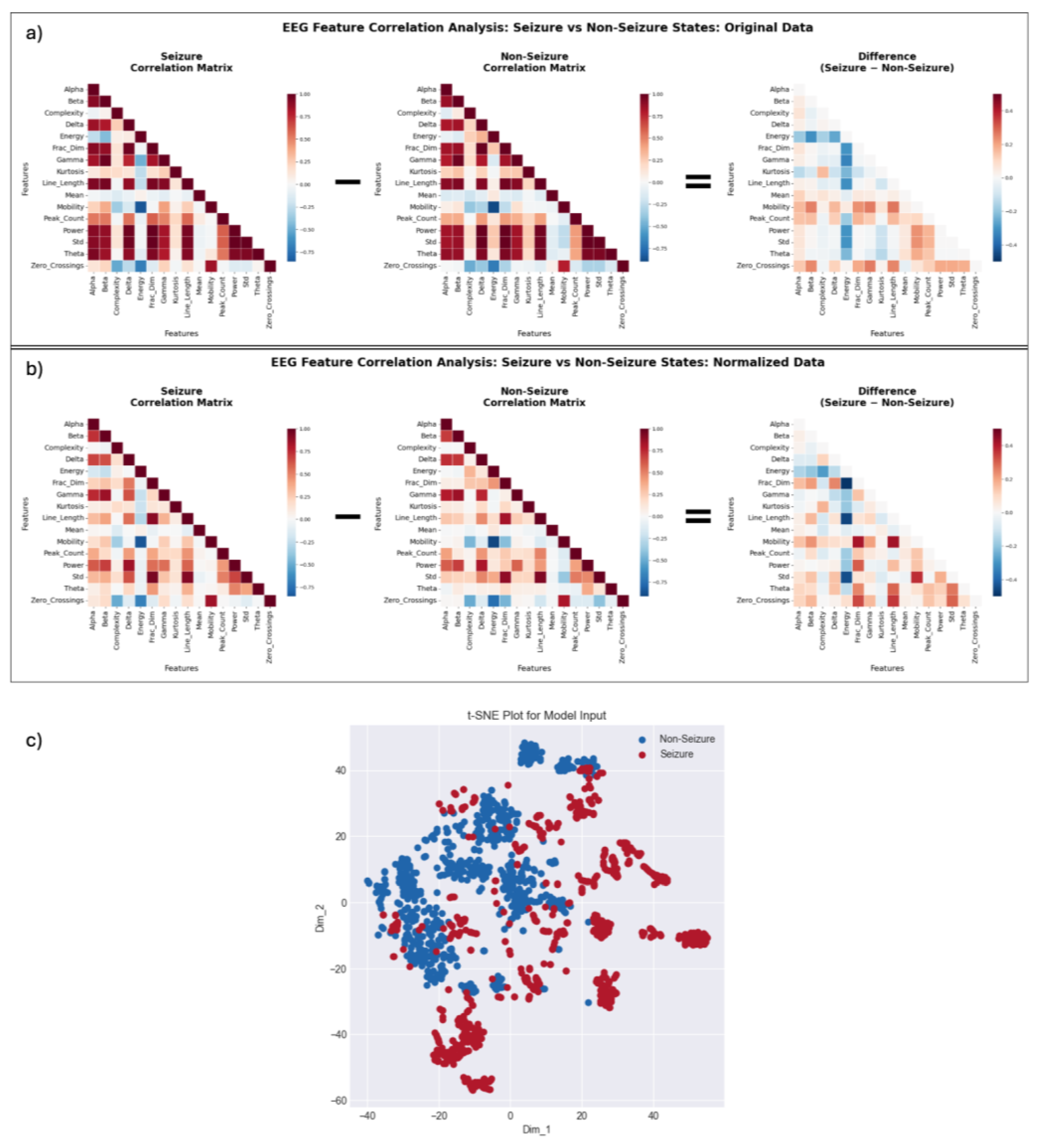
Figure 4.
Model-based feature importance for seizure detection. SHAP-based feature ranking across gradient boosting models. (a) XGBoost. (b) LightGBM. (c) CatBoost. (d) Averaged SHAP importance across all models, consistently identifying complexity, line length, gamma, and beta as highly discriminative features across EEG channels.
Figure 4.
Model-based feature importance for seizure detection. SHAP-based feature ranking across gradient boosting models. (a) XGBoost. (b) LightGBM. (c) CatBoost. (d) Averaged SHAP importance across all models, consistently identifying complexity, line length, gamma, and beta as highly discriminative features across EEG channels.
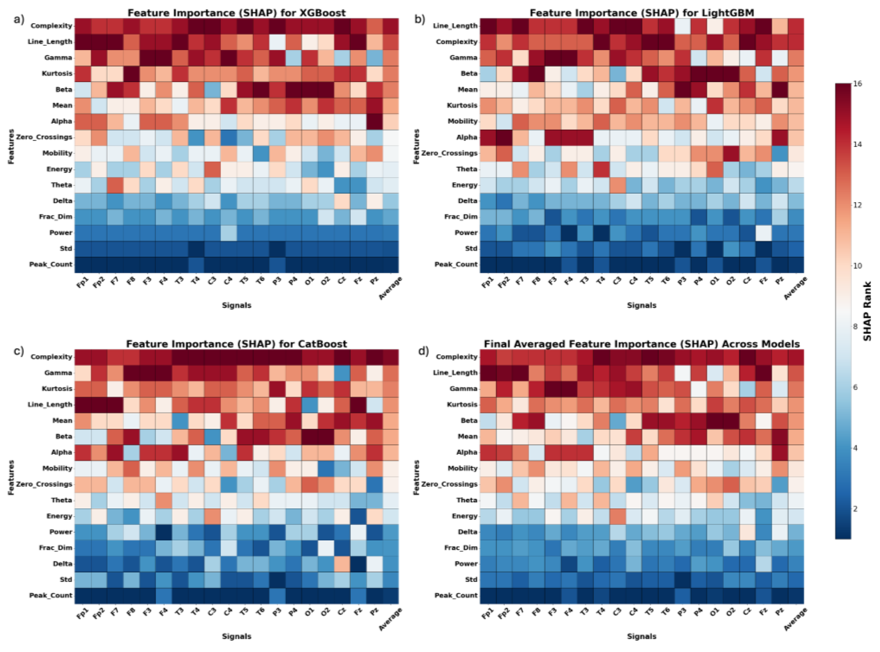

Table 1.
Table 1. Results of experimentation with XGBoost(XGB), CatBoost(CB), LightGBM(LGBM), RUSBoost(RUSB), Balanced-Random-Forest(BRF) and Ensemble model(ESBL).
Table 1.
Table 1. Results of experimentation with XGBoost(XGB), CatBoost(CB), LightGBM(LGBM), RUSBoost(RUSB), Balanced-Random-Forest(BRF) and Ensemble model(ESBL).
| Model Name | Accuracy (%) | Sensitivity (%) | Specificity (%) | ROC | FP/ Hr. | ||||
| Train | Test | Train | Test | Train | Test | Train | Test | ||
| XGB | 99.51± 0.54 | 98.76±0.57 | 95.23± 0.68 | 54.80± 8.48 | 99.57± 0.55 | 99.32± 0.61 | 0.99± 0.005 | 0.92±0.016 | 0.34 |
| CB | 97.12± 2.21 | 96.48± 2.12 | 95.83± 1.49 | 68.29± 6.51 | 97.14± 2.23 | 96.84± 2.18 | 0.99± 0.002 | 0.92±0.018 | 0.6 |
| LGBM | 98.62± 1.33 | 97.93±1.31 | 95.44± 1.57 | 62.87± 8.18 | 98.66±1.34 | 98.38± 1.36 | 0.99± 0.004 | 0.92±0.017 | 0.47 |
| RUSB | 91.22± 8.38 | 91.14± 8.36 | 43.46±32.25 | 41.00±31.95 | 91.82± 8.85 | 91.78±9.83 | 0.88±0.029 | 0.84±0.027 | --* |
| BRF | 90.21± 1.99 | 90.06±2.02 | 82.65± 2.28 | 74.45± 3.17 | 90.31± 2.01 | 90.26± 2.03 | 0.94±0.012 | 0.89±0.015 | --* |
| ESBL | 98.97±0.91 | 99.64± 0.74 | 95.87±0.52 | 89.00±11.00 | 99.01±0.93 | 99.78± 0.62 | 98.27±0.23 | 0.94±0.007 | 0.427 |
* Misses the real seizures completely, marks all segments as non-seizure. Not possible to calculate accurate FP/Hr.
Disclaimer/Publisher’s Note: The statements, opinions and data contained in all publications are solely those of the individual author(s) and contributor(s) and not of MDPI and/or the editor(s). MDPI and/or the editor(s) disclaim responsibility for any injury to people or property resulting from any ideas, methods, instructions or products referred to in the content. |
© 2026 by the authors. Licensee MDPI, Basel, Switzerland. This article is an open access article distributed under the terms and conditions of the Creative Commons Attribution (CC BY) license (http://creativecommons.org/licenses/by/4.0/).
Copyright: This open access article is published under a Creative Commons CC BY 4.0 license, which permit the free download, distribution, and reuse, provided that the author and preprint are cited in any reuse.


