Submitted:
19 April 2026
Posted:
21 April 2026
You are already at the latest version
Abstract
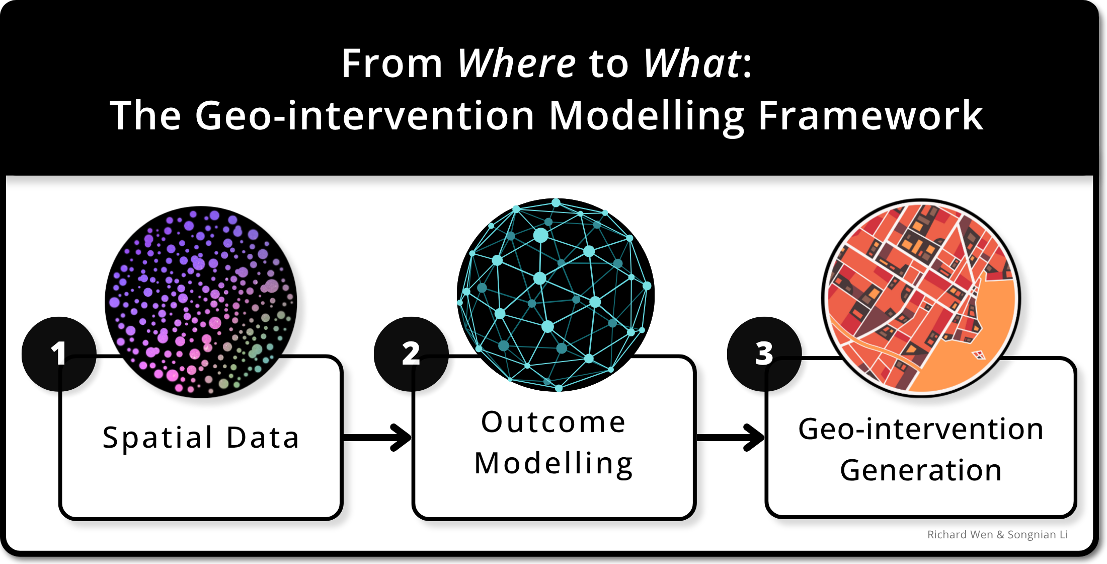
Interventions implemented in geographic space (geo-interventions), have had success in reducing preventable deaths across the world. However, many studies supporting geo-interventions have focused on where to implement them rather than what they are. In this paper, we answer how to model and generate geo-interventions using spatial data, providing what these geo-interventions are and where to apply them. We defined geo-intervention modelling as a problem of optimizing actions and their locations, given the objective of maximizing predicted outcomes. To solve this, we produced a framework for transforming spatial data to model potential actions for generating geo-interventions. Finally, we conducted a case study of reducing traffic collisions in Toronto, Canada, to demonstrate the framework, which produced a machine learning model that discovered geo-interventions modifying red light camera, transit shelter, and wayfinding infrastructure predicted to reduce collisions by 5.7%. We highlight the importance of the framework for bridging research and practice through unified understanding, actionable outputs, human guidance, and iterative refinement. With recent advances in big data and artificial intelligence, we envision an acceleration in the discovery of geo-interventions, and emergence of interdisciplinary work towards predicting accurate and precise future real-world outcomes at scale.
Keywords:
geo-interventions
; geospatial framework
; spatial decision support
; geographic information systems (GIS)
; big data analytics
; predictive modelling
; spatial optimization
; machine learning
; spatial data science
; urban analytics
1. Introduction
Over a million deaths occur every year from preventable causes, such as traffic collisions [1] and homicide [2]. Interventions implemented in geographic space, such as hotspot policing [3] and traffic camera monitoring [4], have had success in greatly reducing the number of preventable deaths. In this paper, these interventions are referred to as geospatial interventions (geo-interventions), which are actions applied to geographic spaces that are intended to alter target outcomes [5,6]. Geo-interventions result in benefits not only for the vulnerable, but also for people living in the surrounding area. A few examples include: reducing the patient load on hospitals [7], improving traffic flow [8], and increasing access to education [9] in relation to reducing traffic and crime related deaths. Geo-interventions are often designed within the constraints of available resources, such as expertise, data, and budget, which are difficult to optimally balance and are heavily reliant on domain expertise [10,11,12]. With high performance computing hardware and the abundance of geospatial data today, analyzing thousands of geo-intervention scenarios within practical periods of time for decision making has become possible [13]. Decision makers are then able to simulate the effects of potential interventions and evaluate outcomes before heavy investments in testing or implementing interventions are spent. This also helps discover more evidence-informed interventions with the available data. Currently, many studies related to geo-interventions only consider a small range of alternative intervention scenarios, constraints, and models predetermined by experts based on experience, research, and experimentation [11,14,15,16,17]. A literature review of over 3000 articles indicated wide use of multi-criteria decision analysis for environmental applications (e.g. waste management, site selection), but revealed heavy dependency on pre-determined scenarios or criteria to evaluate alternative geospatial outcomes [18]. Another similar review of 300 articles demonstrated that decision makers must provide criteria and preference information supplied by experts or stakeholders, rather than systems producing them autonomously [19]. The reliance on experts create difficulty in comparing results and approaches in a standardized manner – leading to issues in optimizing interventions, while leveraging all available data and models. In addition, these studies often identified where to implement geo-interventions with computer models, but to the best of our knowledge, seldom identify what these geo-interventions are [20,21,22,23,24,25]. A recent review of 58 articles [26] and a past review of over 300 articles [11] on spatial analysis for health research highlighted that geospatial approaches primarily focus on identification of spatial patterns, but seldom focus on prescriptive actions or interventions. For example, spatial clustering techniques are used to locate road traffic collision hotspots, but what actions can be taken to decrease road traffic collisions at these hotspots (e.g., deploying traffic enforcement devices, reducing road widths) are often left to decision makers and experts to identify prior or post analysis. Lastly, our past review of 136 articles on spatial decision support systems found that studies leveraging Geographic Information Systems (GIS) were mostly theoretical or experimental, lacking evidence of usefulness to indicate practical success [20]. Thus, we emphasize the importance of not only modelling spatial phenomena, but rather how these phenomena can be altered to influence the real world.
This paper aims to provide a generalized modeling framework for automatically generating geo-interventions using geospatial data for a target outcome, without defining these geo-interventions prior or post analyses. Specifically, the following research questions are answered: (Q1) how do we model geo-interventions? (Q2) how do we generate geo-interventions? and (Q3) how do we apply the geo-intervention generation framework using available models and data? These research questions are answered with the following research contributions respectively: (C1) A framework component for using predictive models to generate geo-interventions for a target outcome, (C2) A framework component for optimizing geo-interventions based on a target outcome, and (C3) A case study of generating geo-interventions to reduce traffic collision deaths and serious injuries in Toronto, Ontario, Canada.
2. Materials and Methods
To answer research questions Q1-3, a three-step approach was taken involving: (1) problem statement, (2) framework specification, and (3) case study. This three-step approach was adapted from a consensus of approaches from [27]. The first step, problem formulation, defined concepts and relationships of actions, locations, and outcomes as they relate to geo-interventions. Research questions Q1-2 were structured into quantifiable optimization problems based on spatial data containing actions and locations. The second step, framework specification, created conceptual components and sub-components based on the definitions of actions, locations, outcomes, and geo-interventions in the problem statement. The definitions of actions and locations were captured as a spatial data component, while the definitions of outcomes and geo-interventions were captured in the outcome modelling and geo-intervention generation components, producing research contributions C1-2 to answer questions Q1-2. These three components formed the geo-intervention modelling framework, which structured the conceptual process of research question Q3. In the third step, a case study in Toronto, Ontario, Canada was designed to produce research contribution C3 by demonstrating use of the framework for a real-world problem, where geo-interventions were generated as locatable infrastructure changes to reduce the number of Killed or Seriously Injured (KSI) individuals, using the geo-intervention modelling framework. Figure 1 visualizes the three-step approach, while Section 2.1 to Section 2.3 detail each of the three steps taken.
2.1. Problem Formulation
This section defines the concept of geo-interventions based on the sub-concepts of actions, locations, and outcomes, while further structuring these defined concepts into quantifiable optimization problems. Geo-interventions are actions that change particular locations or areas in an attempt to produce desirable outcomes in the context of specific decision-making problems, consisting of three concepts seen in Figure 2 [28]:
- Actions: the actions that change entities or phenomena at certain locations or in certain areas (e.g., addition of traffic lights and reduction in road widths)
- Locations: the target locations or areas that actions in are applied to for producing a desirable outcome in the context of decision-making (e.g., neighborhoods with high traffic collisions and streets with high-speed limits)
- Outcomes: the outcomes from applying actions to change the locations or areas in 2. (e.g., reduced traffic collisions and improved traffic flow)
The problem of generating geo-interventions then becomes searching for actions at target locations that influence outcomes in a desired manner. For example, reducing road widths (the action) on streets with high traffic collision rates (the locations) to decrease road traffic injuries (the desired outcome) [29,30,31,32]. Section 2.1.1 to Section 2.1.4 structure the problem of generating geo-interventions by quantifying the three concepts (actions, locations, and outcomes), and their interactions into optimization functions representing desired outcomes.
2.1.1. Actions
Entities, phenomena, and their characteristics in space can be represented as a set of variables containing adjustable values. Actions are then the increase or decrease in these values, indicating changes applied to the entities, phenomena, or their characteristics. For example, a road contains a width and length as two variables with two values and (and indices and respectively) representing the characteristics of a road entity. A change in road width and length values and represent the actions. Thus, a series of actions for variable can be defined as changes for a series of variables , representing entities, phenomena, or their characteristics:
2.1.2. Locations
Each series of actions has a unique location, which is referred to with an index value referencing a set of paired values containing coordinates in space. These coordinates form spatial objects (point, line, polygon) in space [33], representing unique locations. Points consist of a pair of coordinates, lines consist of an ordered set of connected points, and polygons consist of an ordered set of connected points with the starting and ending points connected together to form an area [34]. A point is represented as a pair of ordered coordinates (e.g., (43.65, -79.38)):
A series of ordered points are then used to represent an th unique location described as either a point, line, or polygon (e.g., (43.65, -79.38), (44, -78), (45, -77)):
Thus, each series of actions has a unique location referenced by index , with its own series of changes per location :
2.1.3. Outcomes
Each outcome is a target entity, phenomenon, or characteristic of interest with a unique location. These outcomes are expressed as a variable with a single value at each location and can be affected by a series of actions at the same location. For example, a series of actions at a location containing road width and length changes can change an outcome representing the number of road traffic collisions at the same location. For simplicity, we assume any observed series of actions influence the outcome at location , where outcome changes depending on actions :
Under this assumption, we then build a model of outcomes by finding a function that most accurately produces outcomes based on actions . This outcome model predicts actual outcome as at locations based on a series of variables :
For simplicity, we say that the outcome model seeks to minimize the error between the absolute value of the actual outcome value and estimated outcome value at locations :
2.1.4. Geo-Interventions
Given that outcomes can be estimated with acceptable error using the outcome model, we can predict these outcomes as when actions on variables are applied:
The actions represent the generated geo-interventions, while the predicted outcomes of those geo-interventions correspond to . The next step then becomes finding the actions that lead to the most desirable predicted outcomes , where the choice of minimizing or maximizing is selected based on the context of the decision-making problem (e.g., it is desirable to minimize road traffic collisions and maximize traffic flow):
Equation (9) is a local optimization problem that seeks to optimize the predicted outcomes for each individual location [35]. However, most studies consist of more than one location, and a global optimization problem is more appropriate [36]. Thus, we include an aggregation metric , which considers all predicted outcomes together:
The aggregation metric is dependent on the context of the decision-making problem. For example, we can sum the number of traffic collisions at each location in the study area using the aggregation function and minimize the result of this value, if the intention was to reduce the number of traffic collisions across the study area. Since the number of locations and actions can be large, it may be infeasible to comprehensively try all values of actions [37,38]. Instead, we may reduce the number of values to try by limiting the locations and actions to subsets and respectively, where these subsets are selected based on the decision-making problem (e.g., locations approved for change by policy makers, actions that are possible according to engineers):
Furthermore, we may also reduce the range of values for each action to be between sensible values , determined by the decision-making problem (e.g., 3-5 meter road width reductions following guidelines, 50-100 meter road length increase due to budget):
2.2. Framework Specification
Based on the problem formulation in Section 2.1, this section specifies conceptual components and their sub-components for the concepts of actions, locations, outcomes, and geo-interventions. Recall research questions Q1-2. For Q1, we produce research contribution C1 as the outcome modelling component, conceptualizing the modelling of geo-interventions by predicting outcomes as a function of variables and actions from spatial data. For Q2, we produce research contribution C2 as the geo-intervention generation component, conceptualizing the generation of geo-interventions produced by the outcome models through the application of optimization algorithms and prior knowledge to limit the range of actions to optimize for. Section 2.2.1 to Section 2.2.3 detail the specifications of the spatial data, outcome modelling, and geo-intervention generation framework components, which are summarized in Table 1.
2.2.1. Spatial Data Specifications
Spatial data, commonly used in GIS, capture entities, phenomena, and characteristics as variables , tying these variables to the real-world by locating them in geographic space as described in Section 2.1.2 [39]. By having records of these variables and their locations through spatial data, we can model these variables and their changes as actions in relation to an outcome for the th location, which solves the problem of representing actions, locations, and outcomes in geo-interventions [40]. Thus, we required that the spatial data component contained variables and their locations , where sub-components were organized into vector data, namely point, line, and polygon type spatial data. We focused on vector data to be the spatial data component as it enabled more flexibility and level of detail in geometric shapes (point, line, and polygon) than raster data, which required consistent square or rectangular pixels with level of detail dependent on the image resolution [41,42]. However, we also required an optional sub-component for incorporating raster data, such that raster data be converted to vector data, as is possible with various GIS data processing methods (e.g., polygon grids [42], edge-tracing [43], object detection [44]). For improving interpretability of the locations for geo-interventions, we also required the inclusion of an optional spatial feature engineering sub-component that creates, modifies, and removes variables based on the available variables and geometry data from the vector sub-components [45,46]. In addition, this sub-component can help standardize points, lines, and polygons into common spatial units of interest (e.g., census boundaries for public health interventions [47], regularized grids for simulating land use change [48]) by creating, modifying, and updating variable values inside each spatial unit [49,50]. This spatial feature engineering process enables the possibility to create additional variables that capture the spatial effects among entities, phenomena, and characteristics by aggregating each record and their variables through spatial proximity and relationships [51,52,53].
2.2.2. Outcome Modelling Specifications
Outcomes can be seen as one of the variables captured in the spatial data, where one of the variables are removed and set as the outcome for modelling. Thus, the outcome modelling component attempts to solve the problem of finding a function that predicts the outcome given the variables from the spatial data , such that the difference between the predicted outcome and actual outcome is minimized as seen in Equation (7) from Section 2.1.3. Similar to concepts of predictive modelling [54] (e.g., machine learning [55], statistical modelling [56]), the outcome modelling component conceptualized how to solve this problem by framing outcome models as a function that processes variables and model parameters into predicted outcomes , which we organized into the four sub-components of variables, parameters, models, and predicted outcomes. The variables sub-component was required to hold records from the output of the spatial data component, where each record contained a point, line, or polygon with one or more variables. The parameters sub-component was required to contain a set of optional values that altered the behavior of models to gain potential benefits, such as improved model performance, interpretability, or efficiency [57,58,59]. The models sub-component was required to process the variables and parameters, discover patterns among these variables that had predictive relationships with a selected outcome, alter its behaviors based on the parameters if applicable, and produce predicted outcomes based on the discovered patterns. The predicted outcomes sub-component was required to hold records consisting of points, lines, and polygons with predicted outcome values from the model. We note that the minimization of predicted and actual outcome differences is a simplification of predictive modelling, as models tend to not generalize well to new data, performing well on training data, but poorly on new unseen data [60]. There is also not a single model that works well for every problem, and the exploration of multiple models can result in improved predictive performance [61]. Thus, we added three additional sub-components of model selection (optional), model metrics, and best model, that held algorithms executing strategies (e.g., cross validation [62]) to evaluate and select the best performing model out of a test of multiple models, using a defined model metric on the predicted outcomes.
2.2.3. Geo-Intervention Generation Specifications
As noted in Equation (8) of Section 2.1.4, generated geo-interventions are actions that can predict outcomes given a model with some error , and can be expressed as . Thus, the geo-intervention generation component ideally generates geo-interventions that contain desirable predicted outcomes, where desirability is measured by some aggregation metric with the goal of maximizing or minimizing this metric . The geo-intervention generation component was organized into five required sub-components of actions, outcome metric, optimization algorithm, best outcomes, and best geo-interventions. The actions sub-component was required to hold values that represented a change in variables , available in the best model sub-component from the outcome modelling component, at different locations . The outcome metric sub-component was an aggregation metric that was required to be selected or defined by the user, representing a measure of the desirable predicted outcome. The optimization algorithm sub-component required that a strategy was selected or defined to find the most desirable outcome, using the best model sub-component from the outcome modelling component, and the actions and outcome metric sub-components. The best outcomes sub-component represented the most desirable predicted outcomes found by the optimization algorithm sub-component, while the best geo-interventions are the associated actions that produced the best outcomes using the best model. In Equation (11) and (12), a set of constraints on the actions and locations reduce the number of actions and locations to more appropriate values based on domain knowledge, saving computation time and likely discovering better geo-interventions [63,64]. Thus, we also included an optional constraint sub-component that limited the range of values in the action sub-component for the optimization algorithm to evaluate. In addition, an optional variable metrics sub-component was included to quantify the association of variables in the best model in relation to the predicted outcomes. These metrics provide information on the strength of association (e.g., variable importance [65], correlation coefficient [66]) to the predicted outcomes, which helps set constraints on actions (e.g., top-n actions with strongest association) and verify domain knowledge assumptions in relation to the actions and best model.
2.3. Case Study Design
Road traffic injuries are among the leading cause of death for Canadians 15 to 49 years of age in 2019, ~8% of all deaths for populations aged 15 to 49 years in Canada [67]. Toronto is one of the largest cities in Canada with over 2 million people in 2021 [68] and approximately 55 fatal traffic collisions per year from 2006 to 2021 [69]. Since 2017, the City of Toronto has initiated the Vision Zero Road Safety strategy to reduce road traffic fatalities, with the goal of reaching zero road injury related fatalities through a safe systems approach [70,71]. The City of Toronto and Toronto Police Services collect and distribute detailed geodata on traffic collisions in Toronto through the City of Toronto Open Data Portal [72] and the Toronto Police Service Public Safety Data Portal [73]. In addition to traffic collision data, the City of Toronto Open Data Portal also provides government curated geodata (e.g., infrastructure and sociodemographic entities), which may be linked to the traffic collision data.
We applied the geo-intervention modelling framework to a case study in Toronto, Ontario, Canada, producing research contribution C3 to answer research question Q3. For the case study, we defined our outcome as the number of Motor Vehicle Collisions (MVC), while our geo-interventions as the changes in city infrastructure. Our objective was to reduce the number of MVCs across the city by identifying modifiable infrastructure-related geo-interventions. We organized the case study around the three components of the geo-intervention modelling framework, namely spatial data, outcome modelling, and geo-intervention generation. Section 2.3.1 to Section 2.3.3 detail the approaches taken for the case study based on these three components.
2.3.1. Spatial Data Approach
Spatial data for the outcome of motor vehicle collisions was recorded by the Toronto Police Services, available on their Public Safety Data Portal [73]. Spatial data for city infrastructure geo-interventions was available on the City of Toronto’s Open Data Portal [72]. We also included crime from the Public Safety Data Portal, and amenities and other locations of interest (e.g., cultural hotspots, places of worship) from City of Toronto’s Open Data Portal, as additional variables to include in the outcome modelling component. A total of 21 datasets with 518 variables (columns) and 1,488,148 spatial entities (rows) were used for the case study as seen in Table 2, where all datasets were of point geometry, except for centrelines.
We spatially aggregated the 21 datasets into regularized vector grids of 10 by 10, 40 by 40, and 80 by 80 cells to improve interpretability and provide simpler visualization of the results. Inside of each cell, spatial entities from each dataset had all variables (columns) aggregated by the following statistics: sum, mean, median, min, max, variance, skew, standard deviation, standard error of the mean, and mean absolute deviation. Depending on the geometry of the dataset and data type of variables inside each dataset, we also applied different additional aggregation processes seen in Table 3.
2.3.2. Outcome Modelling Approach
For the case study, we applied Automated Machine Learning (AutoML) for the outcome modelling component as it automates several sub-components related to improving model performance, including the selection of variables, parameters, and models [95]. We tested two python packages for AutoML: auto-sklearn and tpot. The package auto-sklearn uses Bayesian optimization [96], meta-learning [97], and ensemble construction [98] to automatically select the best model from a test of several models and parameters [99,100]. The package tpot uses genetic programming [101] to automatically optimize and design machine learning pipelines through pipeline operators, including the operations of feature engineering, model selection, and parameter tuning [102]. For the variables sub-component, the output of the spatial feature engineering sub-component from the spatial data component was used, while the models sub-component contained both auto-sklearn and tpot models, which automated the parameters and model selection sub-components given a minute to build models each. For the metrics sub-component, we used Mean Absolute Error (MAE) [103], an aggregate measure of the errors between the actual and predicted outcomes, representing the MVCs. Thus, the best model sub-component was determined by the auto-sklearn and tpot models, which automate parameter tuning, model selection, and variable selection/creation based on the MAE metric.
2.3.3. Geo-Intervention Generation Approach
After the best model for predicting MVCs was found using the outcome modelling component, it was used for the generation of geo-interventions based on a change of variable values, representing actions, used in the best model. Thus, the actions sub-component represented increases or decreases to the variable values, containing changes to infrastructure, amenities, crime, and other locations of interest, for the best model. The variable metrics sub-component contained variable importance metrics [65] from the best model, which provides a measure that can be used to rank the most to least influential variables corresponding to the predicted MVCs. We then used Bayesian optimization [96] as the optimization algorithm sub-component to find the best outcomes and geo-interventions, based on the constraints and largest reduction in predicted MVCs. The best outcomes sub-component represented the most optimal reduction in MVCs, while the best geo-interventions component represented the associated increases or decreases in infrastructure-related variables (actions) that led to the best outcomes. For the constraints sub-component, we limited the number of optimization iterations to 1000, along with 1 initial iteration containing the actual variable values from the data, and 100 random iterations to diversify the optimization search space, for a total of 1101 iterations. We also limited the variables for the optimization algorithm to the top three most important modifiable infrastructure variables (determined by the variable importance metric), which was the top three most important variables of the automated speed enforcement cameras, watch your speed devices, red light camera, police facilities, ambulance stations, bicycle parking, transit shelters, wayfinding structures, schools, and childcare centers datasets. In addition, we also included location constraints for two scenarios: (1) areas where the top traffic-related variable had higher than average values, and (2) areas where the top three infrastructure-related variables had lower than average values. In scenario one, we limited optimization to areas with higher-than-average levels of traffic, while in scenario two, we limited optimization to areas with scarcity of important infrastructure for reducing MVCs. We used these scenarios to demonstrate the importance of domain knowledge (e.g., knowing which areas to apply geo-interventions), and its effects on finding the best outcomes and geo-interventions.
3. Results
After applying the three-step approach described in Section 2, we developed the geo-intervention modelling framework and conducted a case study to demonstrate the framework. The geo-intervention modelling framework answered research questions Q1-Q2. For Q1, the framework structured a data modelling process to create prediction models for a target outcome associated with potential geo-interventions, while for Q2, the framework transformed the problem of generating geo-interventions into a global optimization task. Finally, the case study applied the framework to reducing MVCs in Toronto, Canada, with infrastructure-related geo-interventions, demonstrating real-world use of the framework to answer research question Q3. Section 3.1 details the geo-intervention modelling framework and Section 3.2 reports the results of the case study.
3.1. Geo-Intervention Modelling Framework
The geo-intervention modelling framework consisted of three components: (1) spatial data, (2) outcome modelling, and (3) geo-intervention generation. The spatial data component received vector spatial data and standardized it into a set of variables that represented phenomena, entities, or their characteristics. The relevant raster sub-component was optionally included as raster data can be processed into vector structured data with various GIS approaches (e.g., polygon grids [42], edge-tracing [43], object detection [44]). The set of variables from the spatial data component were then used to build models that predicted a target outcome in the outcome modelling component. Here, a model’s accuracy was measured by a metric on the predicted outcomes. This component was divided into two main sub-component processes of models and model selection. Optionally, parameters can be included in each model to adjust model behaviors, with the goal of improving model performance. The models sub-component’s objective was to discover patterns in the variables that can predict an outcome variable with performance measured by the model metric sub-component. If more than one model was built, the model selection sub-component must be defined with a selection strategy or algorithm (e.g., cross validation [62], selecting the model with the best model metric value) based on the predicted model outcomes and model metrics. This model selection process results in a best model being selected to generate geo-interventions in the geo-intervention generation component. This component consisted of sub-components that formed an optimization problem, where the actions sub-component was optimized based on the constraints and outcome metric sub-components. The optimization algorithm process searched for the most optimal outcome metric value given the actions and optional constraints sub-components. The actions sub-component contained changes to the best model’s variables to produce a set of predicted outcomes associated with those changes, while the constraints sub-component contained limitations on the possible actions to optimize for based on prior knowledge. The outcome metrics sub-component sets the objective for the optimization algorithm sub-component, in which a measure is defined based on the predicted outcomes, and a minimization or maximization objective is chosen for the algorithm based on this measure. The optimization algorithm sub-component produced the best outcomes and geo-interventions sub-components based on optimizing for the selected outcome metric, which represents the generated geo-interventions and its associated predicted outcomes. These geo-interventions represented the most optimal actions for each of the locations to produce the optimal predicted outcomes, given the constraints set. Appendix A illustrates minimal examples of the three framework components for better understanding, while Appendix B provides common considerations when defining and applying framework components.
Figure 3.
Geo-intervention modelling framework.

3.2. Case Study
Regression-based AutoML models auto-sklearn and tpot were built for each of the three set of standardized grids, which produced six models (two for each 10 by 10, 40 by 40, and 80 by 80 grid). Out of the six models, the 80 by 80 grid autosklearn model had the best performance (lowest MAE=82.95), while the 10 by 10 grid autosklearn model had the worst performance (highest MAE=1241.93). The performances improved with higher cell counts from 40 by 40 to 80 by 80 grids, with the greatest improvement seen in 10 by 10 to 40 by 40 grid models (-1039 and -951 MAE for autosklearn and tpot respectively). The 80 by 80 grid autosklearn model was selected as the best model for the geo-intervention generation component. The performance of the six models by MAE is shown in Figure 5. An overview of the case study process, applying the geo-intervention modelling framework, is visualized in Figure A1 of Appendix C.
With the 80 by 80 grid autosklearn model as the best model (lowest MAE=82.95), permutation variable importance was calculated for 1408 variables used in the model [104]. The top 25 most important variables from the best model are shown in Figure 6. The most important variable was the number of arterial roads, followed by the number of red light cameras, transit shelters, and crime occurrences involving pointing a firearm. The rest of the variables with variable importance lower than 0.005 were mostly related to traffic volumes and crime occurrences, with a few related to infrastructure (wayfinding, fire hydrants, public art locations, litter receptacles), and one related to the curvature (sinuosity) of road centrelines. The most important traffic volume related variable was traffic_eb_cars_l_sum, the total volume of left-turning eastbound cars. This variable was selected for defining the higher than average traffic areas constraint for scenario one.
The top 25 most important infrastructure-related variables are shown in Figure 7. Asides from the number of red light cameras and transit shelters being the top variables, the number of wayfinding structures, fire hydrants, public art locations, and litter receptacles were among the top most important infrastructure-related variables. Other variables with variable importance less than 0.002 were related to bicycle, Watch Your Speed (WYS) program, school, and cultural hotspot infrastructure. The top three infrastructure variables selected as the actions for scenarios one and two were the number of red light cameras, the number of transit shelters, and the number of wayfinding structures according to their variable importance.
Geo-interventions were generated using the 80 by 80 grid autosklearn model, 1101 iterations of Bayesian Optimization, and the top three most important infrastructure variables, namely the red-light camera, transit shelter, and wayfinding structure counts. Recall that in scenario one, Bayesian Optimization was constrained to grid cells with higher-than-average traffic, while in scenario two, optimization was constrained to grid cells with lower than average red light camera, transit shelter, and wayfinding structure counts. In scenario one, the best geo-intervention occurred with a predicted 554,584 MVC, a reduction of 33,606 (5.7%) compared to the initial 588,190 MVC, while in scenario two, none of the iterations resulted in a reduction in predicted MVC. See Appendix C for details on the iterations to find optimized geo-interventions for each scenario. In scenario one, changes in red light cameras were spread out away from the downtown Toronto area, changes in transit shelters were more concentrated in the downtown area, and changes in wayfinding structures were mostly concentrated in the downtown area and along the center and lower portions (Figure 8). Similarly, the changes in predicted MVC were more concentrated in the downtown area and more spread out away from the downtown core. However, predicted reductions in MVC were seen more in the western than eastern portion of the city.
4. Discussion
This section discusses the considerations, advantages, disadvantages, limitations, and future research directions relevant to the geo-intervention modelling framework and the case study from the results in Section 3. Section 4.1 highlights several advantages from incorporating the geo-intervention modelling framework as a foundation for discovering data-driven geo-interventions in research and practice. The geo-intervention modelling framework provides adaptability and generalizability across disciplines, accelerating the transformation of research into practice by improving human trust through user guided experimentation and design. Section 4.2 discusses the disadvantages of applying the geo-intervention modelling framework related to time and knowledge. The major disadvantages of the geo-intervention modelling framework lie in the omission of very recent advances in modelling approaches and big data, which have been still developing, but rapidly emerging throughout the fields of artificial intelligence and GIS. Section 4.3 discusses the major limitations of the geo-intervention modelling framework relative to validating generated geo-interventions, and lack of empirical evidence for the utility of the framework. The limitations reveal the need for interdisciplinary research of geo-interventions, encouraging the collection of geo-intervention verification data and promoting more studies focused on geo-interventions to further strengthen the framework in the future. Finally, Section 4.4 highlights research opportunities to improve the geo-intervention modelling framework, and long-term visions relative to developments in the framework. These opportunities follow recent shifts towards data-driven decision-making and the incorporation of interdisciplinary expertise into research, both enabled by the rapid advances in artificial intelligence and large-scale computing infrastructure available today.
4.1. Advantages
4.1.1. Bridging Research and Practice
Common GIS modelling and AutoML techniques focus on quantitative approaches based on theory [20], but often do not consider the importance of practitioner knowledge [105,106]. The geo-intervention modelling framework bridges the gap of research and practice through the incorporation of past knowledge from experience or literature into technical modelling processes. For example, applying knowledge from experience about the outcome and its variables to constrain the geo-interventions to actions and areas from practice known to influence the outcome. As most models do not hold knowledge or reasoning of feasibility in relation to the decision-making problem, knowledge from practitioners and experts is invaluable in adjusting the geo-interventions for feasibility [107,108]. Thus, it is not the most optimal solution that is often desired, but the most feasible one, given available resources, that is adequate for implementation in the real world [109]. Results from GIS research are also made more feasible and easier to adopt in the real-world through knowledge from practitioners, encouraging collaboration between academia and industry practice, notably seen in fields like implementation science [110]. Implementing interventions in case studies may require large investments and commitments, with the risk of undesirable or minimal results [111]. Predicting the effects of geo-interventions under feasibility considerations, without directly implementing them, reduces risk in investment and enables exploration of a larger range of alternatives for practice, including innovations in research that have yet to reach practice.
4.1.2. Adaptability and Generalizability
The geo-intervention modelling framework is built as a system of three modular components, spatial data, outcome modelling, and geo-intervention generation, such that each component may be used individually if the input is satisfied. Thus, these components may be used in other modelling frameworks or systems, while being applied to various domains when spatial data is available. For example, we may apply the framework into public health intervention studies to consider spatial data and geo-intervention generation, incorporating more precise and locatable health interventions [112]. Another example is to modify existing GIS frameworks, where we integrate the third geo-intervention generation component to frameworks where the scope of the research is to predict outcomes or events (e.g., traffic event detection [113], predicting urban traffic air pollution [114]). Here, the predictive model can be used as the outcome model for geo-intervention generation, incorporating expert knowledge to examine feasibility through the simulation of changes to input variables and predicted outcomes in different areas. In addition, each framework component may be defined to either sensible defaults or changed to adapt to situations involving differences in resources, user requirements, and expertise [115]. As the concept of geo-interventions is broad and solely requires the transformation of spatial data into outcome models, the framework can be generalized to various domains (e.g., public health [116], environmental science [117], crime [17,118]) and updated for new models or situations, such that the decision-making problem follows the concepts of geo-intervention related actions, locations, and outcomes.
4.1.3. Improving Human Trust
Human guidance of the geo-intervention generation component is crucial in discovering feasible geo-interventions. Major barriers in adopting spatial decision support systems and machine learning are user mistrust for decision-making and lack of technical expertise [105,119]. Both barriers are tied to improve understanding and reducing complexity with engagement and transparency to increase trust for decision-making [119,120]. The geo-intervention modelling framework helps improve understanding by simplifying the modelling of geo-interventions to three major components that are generalizable to any domain, enabling non-experts with practical knowledge to be involved in the process. For example, non-experts can collaborate with engineers or developers to evaluate what data is used for the spatial data component, what considerations should be incorporated into the metrics of the outcome modelling component, and what actions and geo-intervention areas are likely to be effective or feasible. Additionally, non-experts can experiment with different scenarios, as done in this paper’s case study, to simulate the effects of different geo-interventions based on their knowledge. This improves trust by introducing user through external validation based on reasoning and past knowledge, supplementing pure quantitative approaches seen in research, to observe if the model behaves as expected with changes to the input variables [121,122]. Furthermore, a standard framework helps users compare different solutions, allowing for evaluation of different intervention ideas among stakeholders, decision-makers, studies, and analyses, which is not commonly addressed due to inconsistencies in intervention design [112]. For geo-interventions to be implemented or adopted, they must not only be feasible and accurate but also trusted by decision-makers. The geo-intervention modelling framework addresses this issue by enabling human feedback and guidance to shape the feasibility of geo-interventions, while leveraging the precision of data models for simulating impacts geo-interventions, removing need for expensive implementation.
4.2. Disadvantages
4.2.1. Temporal and Real-Time Data
The geo-intervention modelling framework did not consider temporal data and their variables, which may be important for modelling datasets that capture temporal phenomena over multiple years or decades. Temporal geodata differ from static geodata, as a dependency on time exists in the data structure and implications [123]. For example, temporal geodata has three dimensions, containing records in space (first and second dimensions) that are also sequentially dependent on time (third dimension), where each record occurs before, during, or after another record. This data can capture the temporal effects of variables and outcomes, as time-based models have been well studied and used for analyzing public health interventions [124,125,126]. For example, it is common to analyze when and how long interventions are expected to be implemented and effective. In addition, temporal geodata is often continuously collected with new records added over time, particularly real-time geodata [127,128,129]. The framework does not consider updates in data or models, and instead relies on re-processing when enough new data is available. This may result in models missing new variables and patterns due to changes over time (e.g. context drift [130]). Integrating approaches for temporal geodata into the geo-intervention modelling framework will enable the modelling of geo-interventions over time and more efficient methods for updating spatial data and outcome models on demand.
4.2.2. Knowledge Transfer
The transfer of knowledge is important in decision-making and modelling to encourage reuse, reproducibility, and collaboration that leads to desirable interventions and outcomes [131,132]. However, the geo-intervention modelling framework does not consider the transfer of knowledge from previous or existing processes and models despite a focus on modularity. Incorporating a standardized manner of knowledge transfer in the framework can promote reuse, reproduction, and sharing of models and related processes [133,134], enabling savings in resources (e.g. computational expenses required to train models [135]), wider adoption to different domains (e.g. easier reuse by various domain experts [136]), and refinement of models and processes that lead to more effective geo-interventions or accurate models (e.g. improvements of adopted models or processes to similar problems in contrast to past studies [137]). Although the framework encourages the application of knowledge to the geo-intervention modelling process, users of the framework may benefit from explicitly defined components or processes for knowledge application and transfer as seen in incremental or transfer learning [138,139] .
4.2.3. Contextual Reasoning
With the recent emergence of Large Language Models (LLMs), computers can generate natural language text similar to human-level reasoning [140,141,142,143]. This has allowed LLMs to produce working programming scripts [144], answer online store inquiries [145], analyze financial market trends [146], and suggest medical diagnoses [147]. As human guidance and knowledge greatly influences the generated geo-intervention quality, there is potential for the integration of LLMs to generate this guidance and knowledge, and perform functions based on it. For example, the LLM may provide common knowledge on what variables influence the outcome, followed by what variables are considered feasible actions, and then finally select them for generating geo-interventions. In this example, the LLM may provide known knowledge on what areas are the most effective and feasible to target from the actions, and limit the generation to these areas. However, it is noted that LLMs are still relatively new and perform similar to the wisdom of the crowds [148], but does not currently reason or operate at the human level for all tasks despite improvements [149,150] (e.g. chain-of-thought [151]), failing simple logic and reasoning tests [152,153]). Nonetheless, the framework does not consider models that offer contextual reasoning, which can be beneficial in ensuring that geo-interventions are feasible at the level of common knowledge amongst experts in the decision-making problem.
4.3. Limitations
4.3.1. Geo-intervention Verification
Due to limited availability of precise intervention data (e.g. historical changes to road design affecting intersection safety, policy shifts applied at certain locations), it was not possible at the time of study to verify that the generated geo-interventions were feasible and effective in the real world. Impact evaluations for interventions often lack data (e.g. erroneous and missing data [154], compatible standards [155], or ethical issues [156]) or sufficiently detailed data (e.g. inadequate time intervals or spatial resolution [157]), while study design alone is not adequate to indicate a successful intervention [112]. This makes it difficult to conclude interventions are effective in studies, as it introduces bias that omits external factors, unrelated to the interventions, that potentially cause beneficial effects [158]. It was also impractical to implement case studies due to the scale and expenses of the unverified geo-interventions, where most interventions are often complex and costly to implement at scale [111]. The difficulties and complexities in sourcing verification data and implementing experimental geo-interventions reveal a need for intervention related datasets, which help verify that models perform to the level of existing interventions.
4.3.2. Empirical Evidence
As this paper’s scope was to introduce the geo-intervention modelling framework, it did not yet have adequate empirical evidence of its use in the real-world, asides from the conducted case study. Evidence of adoption and utility of the framework is crucial to prove its effectiveness in variety of fields, in practice, and for different audiences. When frameworks are increasingly used in research and practice, hidden issues and limitations are further uncovered from various perspectives and impact evaluations [159], allowing for innovative improvements that create better frameworks [160]. However, this is a long and complex process, involving collaborative work in uptake and dissemination (e.g. development of software, advertising, guidance materials, partnerships) [161]. Nonetheless, frameworks are generally introduced, before empirical evidence follow, which presents a common limitation of newly introduced methodological frameworks.
4.4. Opportunities
4.4.1. Framework Extensions
Research in extending the geo-intervention modelling framework with additional components aids in establishing a standard of understanding with the base components, while allowing for work into addressing the framework’s disadvantages and limitations. For example, temporal sub-components (e.g. feature engineering temporal variables, time-series models, sequential generation of geo-interventions) may be added to all components to enable time-relevant geo-interventions. Another example involves applying the framework to different domain-specific problems. This helps identify component additions and modifications that create sub-frameworks specific to problems in particular domains (e.g. public health, transportation engineering, planning), assisting in better knowledge transfer. Incorporating LLMs as optional sub-components for knowledge support will also mediate the lack of contextual reasoning (e.g. ranking feasibility of actions from variables, evaluating practicality of geo-interventions, suggesting approaches for outcome modelling and spatial feature engineering). Work towards creating framework extensions will address noted issues in the framework related to temporality, knowledge transfer, and contextual reasoning, while offering a standardized manner for improving the framework when future issues arise.
4.4.2. Precision Geo-Interventions
The geo-intervention modelling framework provides a foundation towards precision geo-interventions, where interventions are precisely located with quantifiable actions and outcomes. Big data has enabled more granular interventions in health, allowing the field of precision public health to target smaller subpopulations among larger populations with sociodemographic information [162]. Similarly, precision geo-interventions enable granular interventions, but across space and with the distinction of generalizing to location, which is applicable to any domain that utilizes spatial data. Thus, practitioners and experts across different domains may use a consistent framework for examining not only interventions in their own domains, but the effects of related or combined interventions outside their domains, which are often not considered [163,164,165]. Examining different interventions on multiple outcomes, rather than a single outcome, is made possible to evaluate their effects, not only for a targeted outcome, but for adverse effects on non-targeted outcomes as well [166]. With recent advancements in artificial intelligence and computing power, geo-interventions may emerge as an important research topic and development in the field of Geographic Information Science (GIScience), particularly as more decision makers incorporate spatial data in their processes, strategies, and overall systems.
4.4.3. Universal Geo-Intervention Platform
The geo-interventions framework provides a standardized framework that can be used across various disciplines, which establishes the opportunity for a universal geo-intervention platform. The effectiveness of interventions vary across different populations locations, and time [167,168], while they are difficult to compare in finer spatial and temporal as intervention data are often stored and disseminated in research papers and reports without interoperable data for standardized comparison [169,170]. Hence, there is much data for developing and monitoring interventions, but not much data about interventions (e.g. resulting outcomes, relevant effects/risks on populations, and actions taken from applying interventions). Thus, it is difficult to directly compare, reuse, reproduce, and share interventions at the quantitative level across different fields of study. With recent developments in geo-foundation models (e.g. AlphaEarth [171,172], population dynamics foundation model [173]), integration, standardization, and searchability of diverse spatial data has improved drastically [174,175,176]. We envision that this will be possible for geo-intervention data as well, providing an open universal technology platform that promotes collaboration among researchers and practitioners to accelerate innovation and application of research to practice.
5. Conclusions
A generalized modeling framework for generating geo-interventions from spatial data is described in this paper with details on how to model and generate geo-interventions while applying the framework. We provided specifications on three major framework components (spatial data, outcome modelling, and geo-intervention generation) that form the framework, based on the concept of geo-interventions defined by the interactions between actions, locations, and outcomes. In addition, we demonstrated an application of the framework for generating infrastructure-related geo-interventions on reducing road collisions in Toronto, Canada. Advantages, disadvantages, and limitations regarding the geo-intervention modelling framework were discussed. Notably, the framework presented advantages in bridging research and practice through flexibility of application across disciplines for better collaboration, and integration of prior knowledge to improve human trust and understanding. However, recently rapid advances in artificial intelligence and large-scale computing have not yet been fully developed and widely adopted. This led to several disadvantages in the framework, where components for temporal data processing, reuse of prior models, and automated contextual reasoning were omitted. Perhaps the largest barriers to adopting the framework lied in the lack of data on geo-intervention and their outcomes to date, along with the application of the framework in more studies, presenting important limitations of this paper. Although the framework was introduced in this paper, it may be improved in the future with initiatives in data collection and collaboration amongst the research and practicing community. Thus, we foresee opportunities to extend the framework by incorporating additional components to address disadvantages, and eventually the development of a universal geo-intervention platform that enables researchers and practitioners to share, extend, reuse, and precisely apply geo-interventions across various disciplines. As innovations shift towards the application of standardized data and interdisciplinary knowledge to decision-making and GIS, future outcomes from proposed actions can eventually be predicted precisely at scale, accelerating discovery of effective interventions that potentially prevent the loss of lives and improve the quality of life across the world.
Author Contributions
Conceptualization, Richard Wen; methodology, Richard Wen, Songnian Li; investigation, data curation, software, writing—original draft preparation, Richard Wen; supervision, funding acquisition, resources, project administration, Songnian Li; writing—review and editing, Richard Wen, Songnian Li. All authors have read and agreed to the published version of the manuscript.
Funding
This work was funded by the Natural Sciences and Engineering Research Council of Canada, grant number RGPIN-2017-05950.
Data Availability Statement
Conflicts of Interest
The authors declare no conflicts of interest.
Appendix A. Examples for Geo-Intervention Modelling Framework Components
To improve understanding for each component of the geo-intervention modelling framework, minimal example data in tabular format and related calculations are illustrated in to Appendix A.2. The Python code for these minimal examples is available on a Github repository [177].
Appendix A.1. Spatial Data Component Example
Table A1 shows a simple example of tabular data representing vector sub-components and processed variables from the spatial feature engineering sub-component. Variables Xi,1…Xi,2 represent the original variables for each location Li, while Xi,1 + Xi,2, Nearesti, Length(Li), and Type(Li) are additional variables from spatial feature engineering, representing the sum of Xi,1 and Xi,2, the index i of the nearest location, the length of the location entity, and the type of the location entity respectively. Here, each location has a set of variables, and the spatial feature engineering process created additional variables to capture spatial relationships and properties.

Table A1.
Example spatial data for the geo-intervention modelling framework.
| i | Xi,1 | Xi,2 | Xi,3 | Xi,1 + Xi,2 | Nearesti | Length(Li) | Type(Li) | Li |
| 1 | 1.25 | 2 | 4 | 3.25 | 2 | 0 | Point | (43, -79) |
| 2 | 2.55 | 4 | 0 | 6.55 | 1 | 1.41 | Line | (45, -79) (44, -78) |
| 3 | 5.75 | 6 | 16 | 11.75 | 2 | 11.09 | Polygon | (46, -77) (47, -80) (48, -75) |
Appendix A.2. Outcome Modelling Component Example
Table A2 expands on Table A1, showing the outcome model as a function of the spatial data provided. A model is built for outcomes Yi as a function of variables Xi,1, Xi,2, Xi,1 + Xi,2, Nearesti, Length(Li), and Type(Li) to produce predicted outcomes with errors ei as the model metrics. Here, the predicted outcomes was selected as variable Xi,3, and excluded as one of the model’s input variables, while was ignored as the index for each unique location.
Table A2.
Example outcome modelling data for the geo-intervention modelling framework.
| i | Xi,1 | Xi,2 | Xi,1 + Xi,2 | Nearesti | Length(Li) | Type(Li) | Yi = Xi,3 | = f(X1 … Type(Li)) | ei = |Yi -| |
| 1 | 1.25 | 2 | 3.25 | 2 | 0 | Point | 4 | 4.59 | 0.59 |
| 2 | 2.55 | 4 | 6.55 | 1 | 1.41 | Line | 0 | 0 | 0 |
| 3 | 5.75 | 6 | 11.75 | 2 | 11.09 | Polygon | 16 | 16.62 | 0.62 |
Appendix A.3. Geo-intervention Generation Component Example
Finally, Table A3, expanding on Table A2, shows a simple example of one iteration of an optimization algorithm, where a set of action values Ai,4 and Ai,5 was applied to variables Xi,1 + Xi,2 and Length(Li) to produce estimated variables and . Here, constraints limited the optimization to only modify variables Xi,1 + Xi,2 and Length(Li) for locations 1 and 2, while Ai,1…Ai,3 would be set to zero (no change) as they were non-modifiable according to the set constraints. The estimated variables were used as input for the best model, producing the associated set of predicted outcomes , which can be evaluated with an outcome metric. For example, given the sum of the predicted outcomes, and the objective of minimizing this sum, the optimization algorithm attempts to adjust actions Ai,4 and Ai,5 to produce the lowest sum given a set number of iterations or when all possible values are explored. In this example situation, the actions Ai,1…Ai,5 that produced the lowest sum would be the best geo-interventions, while its predicted outcomes would be the best outcomes.
Table A3.
Example geo-intervention generation data for one iteration of the optimization algorithm.
| i | Xi,1 + Xi,2 | Length(Li) | Ai,4 | Ai,5 | = (Xi,1 + Xi,2) + Ai,4 | = Length(Li) + Ai,5 | = f( …) |
| 1 | 3.25 | 0 | +7 | +2 | 10.25 | 2 | 4.25 |
| 2 | 6.55 | 1.41 | -3 | -1 | 3.55 | 0.41 | 7.1 |
Appendix B. Considerations for Geo-Intervention Modelling Framework Components
When applying the geo-intervention modelling framework, several considerations relative to data processing, modelling, and optimization are needed to adapt the frame-work to different problem contexts. This appendix describes common approaches and their importance for selecting spatial feature engineering, outcome modelling and evaluation, and geo-intervention optimization components. Careful consideration of these components may improve outcome modelling performance, inference, and generated geo-interventions, while balancing computing resources and adapting the entire system to better fit decision-making context.
Appendix B.1. Spatial Feature Engineering Considerations
Depending on the input spatial data structures (e.g. lines, points, polygons), various spatial feature engineering methods may be used to extract more informative features, or remove them, for modelling. For example, we may create additional features that capture spatial information, using spatial relationships (e.g. nearest neighbor, distance decay), geometry (e.g. line curvature, polygon area), or spatial aggregation [49,178] (e.g. units per square kilometer, sum of nearest neighbors). Another common example is to remove any input variables that are directly related to the outcome (e.g. variables aggregated using the outcome variable). The decision to create and remove these spatial features may rely on computational resources (e.g. memory limits, storage, parallel processing, expenses [179,180,181]), past knowledge (e.g. literature, experience, expertise [182]), or an algorithmic process (e.g. feature selection [183]). Thus, the efficiency of data processing for spatial features needs to be considered using past knowledge and expertise. Although spatial features are often not included directly in datasets, they enable outcome models to account for spatial effects that are not present in non-spatial data, which can potentially improve model performance or uncover important hidden variables for inference.
Appendix B.2. Outcome Modelling and Evaluation Considerations
The choice of outcome models and evaluation metrics determine how accurate predicted outcomes from geo-interventions are to the input data, and if the outcome is represented adequately according to the decision maker’s perspective. Models are often selected based on prior knowledge of the input variables and outcome (e.g. statistical modelling), but recent advances in machine learning enabled the automatic selection of models, without prior knowledge, as a tradeoff between processing time and performance (e.g. AutoML) [61,184,185,186]. While selecting models based on prior knowledge generally offers improved interpretability and computational efficiency on smaller datasets, automatic selection approaches may provide better performance and test a larger variety of models to provide empirical evidence [187,188]. Ideally, a hybrid approach may be used, where trusted models from prior knowledge can be used as baseline comparisons to more automated approaches to produce stronger empirical evidence for the selection of models. In addition, the choice of metrics needs to reflect the decision-making problem, related risks, and the characteristics of the input data [189,190]. Considering an evaluation metric involves identifying the outcome, how to quantify that outcome to be interpretable for the decision-making problem, and whether an increase or decrease in those quantities are desired. Data characteristics and related risks influence the validity of the metric for practical use, as imbalances in the outcome variable and side effects from related risks greatly influence whether the model and its predictions are valid in the real world. For example, the F1 score is used to address issues where models overfit to one or a small number of categories, providing a false interpretation of high performance [191]. Another example involves incorporating outcome effects on vulnerable populations (e.g. disabled, low-income families) and equity (e.g. distribution of benefits or damages from outcome across areas and sub-populations) in evaluation metrics to account for risks [192,193,194]. In this example, we may also consider multiple outcome sub-models with a unifying metric to address the target outcome (e.g. road traffic injuries), and their outcome effects (e.g. vulnerable populations and equity). With adequate computational resources, efforts on the choice of metrics may provide more benefit than efforts spent on the choice of models as automated modelling approaches develop, and more non-expert users are able to apply these models.
Appendix B.3. Optimization Algorithm and Guidance Considerations
After creating an outcome model to generate geo-interventions, an optimization algorithm is required to approximate the best geo-intervention from a constrained set of alternative geo-interventions. Selecting and guiding this algorithm generally helps in finding more desirable outcomes, as it limits the extremely large search space (set of alternative geo-interventions), where it is impractical to explore all possible options [195,196]. First, an optimization algorithm must be selected. Common choices are sequential [197], grid [198], random [199], Bayesian [200], evolutionary [201], gradient descent [202], and particle-swarm search [203], where these algorithms outperform brute-force and search under similar time limits. Ideally, experimenting with a combination of different optimization algorithms under reasonable time limits, before committing more resources, is desirable, as it provides empirical evidence for selecting an algorithm given the model, dataset, and various constraints. For example, grid, random, Bayesian, and evolutionary algorithms may be run in parallel for two hours, while the algorithm that yields the best geo-intervention is chosen to be run for several days. Here, computational resources, potential for parallelization, and hybrid algorithms may also be considered. Computational resources and parallelization may allow certain algorithms to explore more options (e.g. parallelized grid or random search [204]), and disadvantage others (e.g. dependency on previously explored options in Bayesian search [96]). There is also possibility in combining algorithms, such as applying random search to initialize better prior options for Bayesian search [199]. Second, guiding the selected algorithm has perhaps the largest influence on finding more optimal geo-interventions, as it defines constraints that drastically both reduce search spaces and improve understanding, as these constraints often represent applied knowledge from expertise in the outcome’s behavior. In the case study, a common relationship is known between traffic volumes and collisions, and thus, two scenarios focused on defining constraints on high and low traffic areas to reduce collisions. In scenario two, low traffic areas had a much larger search space and did not result in any geo-interventions that would reduce collisions. In scenario one, high traffic areas had lowered the search space, and resulted in several geo-interventions that lowered collisions, which is consistent with past knowledge on traffic collisions [205,206,207]. Additionally, the number of variables were limited to the top three most important infrastructure variables, further limiting the search space to represent modifiable phenomena in the real world. Here, the search space was limited by reducing the number of variables and the areas in which geo-interventions can be applied. Careful consideration is needed in limiting the search space to modifiable variables and spatial areas relative to the decision-making context. Hence, the decision maker’s knowledge is crucial in limiting the search space to guide the optimization algorithm towards generating both more practical and effective geo-interventions that can be applied in the real world.
Appendix C. Case Study Details
This appendix provides details on the case study in Section 3.2, namely the overall process applied in the case study and the optimization iterations found in the outcome modelling component. Figure A1 illustrates an application of the geo-intervention modelling framework in Figure 3 to the case study by specifying each framework component and sub-component. In the first spatial data component, data is spatially aggregated into a standard format as described in Section 2.3.1. In the second outcome modelling component, AutoML models were built to predict MVCs and find the best model as described in Section 2.3.2. Lastly, the geo-intervention generation component uses Bayesian optimization, given several constraints described in Section 2.3.3, to generate optimized geo-interventions using the best model found in the previous outcome modelling component. Figure A2 to A3 visualize the reduction in MVCs when applying Bayesian optimization to the top three most important infrastructure variables the best model found in the case study. For scenario one, the optimal reduction of MVCs was found at iteration 983, while for scenario two, there was no reduction of MVCs found throughout all 1101 iterations since the initial iteration.
Figure A1.
Application of the geo-intervention modelling framework for the case study.

Figure A2.
Bayesian optimization iterations for scenario one using 80 by 80 grid autosklearn model.

Figure A3.
Bayesian optimization iterations for scenario two using 80 by 80 grid autosklearn model.

References
- World Health Organization Global Status Report on Road Safety; Geneva, 2018.
- United Nations Office on Drugs and Crime Global Study on Homicide; Vienna, 2019.
- Braga, A.A.; Schnell, C. Evaluating Place-Based Policing Strategies: Lessons Learned from the Smart Policing Initiative in Boston. Police quarterly 2013, 16, 339–357. [Google Scholar] [CrossRef]
- Yang, B.-M.; Kim, J. Road Traffic Accidents and Policy Interventions in Korea. Injury Control and Safety Promotion 2003, 10, 89–94. [Google Scholar] [CrossRef] [PubMed]
- Richard Wen Generative Design of Geospatial Interventions With Automated Machine Learning and Bayesian Optimization; Toronto Metropolitan University: Toronto, 2023.
- A Ross, D.; G Smith, P.; H Morrow, R. Types of Intervention and Their Development. In Field Trials of Health Interventions, 3rd ed.; Oxford University Press, 2015. [Google Scholar]
- Bonnet, E.; Lechat, L.; Ridde, V. What Interventions Are Required to Reduce Road Traffic Injuries in Africa? A Scoping Review of the Literature. PLOS ONE 2018, 13, e0208195. [Google Scholar] [CrossRef] [PubMed]
- Bunn, F.; Collier, T.; Frost, C.; Ker, K.; Roberts, I.; Wentz, R. Traffic Calming for the Prevention of Road Traffic Injuries: Systematic Review and Meta-Analysis. Injury Prevention 2003, 9, 200–204. [Google Scholar] [CrossRef]
- Yang, B. GIS Crime Mapping to Support Evidence-Based Solutions Provided by Community-Based Organizations. Sustainability 2019, 11, 4889. [Google Scholar] [CrossRef]
- Boulos, M.N.K. Towards Evidence-Based, GIS-Driven National Spatial Health Information Infrastructure and Surveillance Services in the United Kingdom. Int J Health Geogr 2004, 3, 1. [Google Scholar] [CrossRef]
- Nykiforuk, C.I.J.; Flaman, L.M. Geographic Information Systems (GIS) for Health Promotion and Public Health: A Review. Health Promotion Practice 2011, 12, 63–73. [Google Scholar] [CrossRef]
- Wang, R.; Murayama, Y.; Morimoto, T. Scenario Simulation Studies of Urban Development Using Remote Sensing and GIS: Review. Remote Sensing Applications: Society and Environment 2021, 22, 100474. [Google Scholar] [CrossRef]
- Elsahlamy, E.; Eshra, A.; Eshra, N.; El-Fishawy, N. Empowering GIS with Big Data: A Review of Recent Advances. In Proceedings of the 2021 International Conference on Electronic Engineering (ICEEM), July 2021; pp. 1–7. [Google Scholar]
- Bailey, P.E.; Keyes, E.B.; Parker, C.; Abdullah, M.; Kebede, H.; Freedman, L. Using a GIS to Model Interventions to Strengthen the Emergency Referral System for Maternal and Newborn Health in Ethiopia. International Journal of Gynecology & Obstetrics 2011, 115, 300–309. [Google Scholar] [CrossRef]
- Franch-Pardo, I.; Napoletano, B.M.; Rosete-Verges, F.; Billa, L. Spatial Analysis and GIS in the Study of COVID-19. A Review. Science of The Total Environment 2020, 739, 140033. [Google Scholar] [CrossRef]
- Ištoka Otković, I.; Karleuša, B.; Deluka-Tibljaš, A.; Šurdonja, S.; Marušić, M. Combining Traffic Microsimulation Modeling and Multi-Criteria Analysis for Sustainable Spatial-Traffic Planning. Land 2021, 10, 666. [Google Scholar] [CrossRef]
- Piza, E.L.; Kennedy, L.W.; Caplan, J.M. Facilitators and Impediments to Designing, Implementing, and Evaluating Risk-Based Policing Strategies Using Risk Terrain Modeling: Insights from a Multi-City Evaluation in the United States. Eur J Crim Policy Res 2018, 24, 489–513. [Google Scholar] [CrossRef]
- Cegan, J.C.; Filion, A.M.; Keisler, J.M.; Linkov, I. Trends and Applications of Multi-Criteria Decision Analysis in Environmental Sciences: Literature Review. Environ Syst Decis 2017, 37, 123–133. [Google Scholar] [CrossRef]
- Malczewski, J. GIS-based Multicriteria Decision Analysis: A Survey of the Literature. International Journal of Geographical Information Science 2006, 20, 703–726. [Google Scholar] [CrossRef]
- Wen, R.; Li, S. Spatial Decision Support Systems with Automated Machine Learning: A Review. ISPRS International Journal of Geo-Information 2023, 12, 12. [Google Scholar] [CrossRef]
- Akbari, K.; Winter, S.; Tomko, M. Spatial Causality: A Systematic Review on Spatial Causal Inference. Geographical Analysis 2023, 55, 56–89. [Google Scholar] [CrossRef]
- Mortaheb, R.; Jankowski, P. Smart City Re-Imagined: City Planning and GeoAI in the Age of Big Data. Journal of Urban Management 2023, 12, 4–15. [Google Scholar] [CrossRef]
- Chen, M.; Claramunt, C.; Çöltekin, A.; Liu, X.; Peng, P.; Robinson, A.C.; Wang, D.; Strobl, J.; Wilson, J.P.; Batty, M. Artificial Intelligence and Visual Analytics in Geographical Space and Cyberspace: Research Opportunities and Challenges. Earth-Science Reviews 2023, 241, 104438. [Google Scholar] [CrossRef]
- Biu, P.W.; Nwasike, C.N.; Tula, O.A.; Ezeigweneme, C.A.; Gidiagba, J.O. A Review of GIS Applications in Public Health Surveillance. World Journal of Advanced Research and Reviews 2024, 21, 030–039. [Google Scholar] [CrossRef]
- Fradelos, E.C.; Papathanasiou, I.V.; Mitsi, D.; Tsaras, K.; Kleisiaris, C.F.; Kourkouta, L. Health Based Geographic Information Systems (GIS) and Their Applications. Acta Inform Med 2014, 22, 402–405. [Google Scholar] [CrossRef]
- Chandran, A.; Roy, P. Applications of Geographical Information System and Spatial Analysis in Indian Health Research: A Systematic Review. BMC Health Serv Res 2024, 24, 1448. [Google Scholar] [CrossRef]
- McMeekin, N.; Wu, O.; Germeni, E.; Briggs, A. How Methodological Frameworks Are Being Developed: Evidence from a Scoping Review. BMC Med Res Methodol 2020, 20, 173. [Google Scholar] [CrossRef]
- Wen, R.; Li, S. Generative Design for Precision Geo-Interventions. Proceedings of the ISPRS Annals of the Photogrammetry, Remote Sensing and Spatial Information Sciences 2022, Vol. X-3-W2-2022, 37–42. [Google Scholar] [CrossRef]
- Manuel, A.; El-Basyouny, K.; Islam, Md.T. Investigating the Safety Effects of Road Width on Urban Collector Roadways. Safety Science 2014, 62, 305–311. [Google Scholar] [CrossRef]
- Ekmekci, M.; Woods, L.; Dadashzadeh, N. Effects of Road Width, Radii and Speeds on Collisions at Three-Arm Priority Intersections. Accident Analysis & Prevention 2024, 199, 107522. [Google Scholar] [CrossRef] [PubMed]
- Godley, S.T.; Triggs, T.J.; Fildes, B.N. Perceptual Lane Width, Wide Perceptual Road Centre Markings and Driving Speeds. Ergonomics 2004, 47, 237–256. [Google Scholar] [CrossRef]
- Rahman, Z.; Memarian, A.; Madanu, S.; Iqbal, G.; Anahideh, H.; Mattingly, S.P.; Rosenberger, J.M. Assessment of the Impact of Lane Width on Arterial Crashes. Journal of Transportation Safety & Security 2017, 1–22. [Google Scholar] [CrossRef]
- Blaschke, T.; Merschdorf, H.; Cabrera-Barona, P.; Gao, S.; Papadakis, E.; Kovacs-Györi, A. Place versus Space: From Points, Lines and Polygons in GIS to Place-Based Representations Reflecting Language and Culture. ISPRS International Journal of Geo-Information 2018, 7, 452. [Google Scholar] [CrossRef]
- Verbyla, D.L. Practical GIS Analysis; CRC press, 2002. [Google Scholar]
- Johnson, D.S. Local Optimization and the Traveling Salesman Problem. In Proceedings of the Automata, Languages and Programming; Paterson, M.S., Ed.; Springer: Berlin, Heidelberg, 1990; pp. 446–461. [Google Scholar]
- Horst, R.; Pardalos, P.M.; Van Thoai, N. Introduction to Global Optimization; Springer Science & Business Media, 2000. [Google Scholar]
- Wolpert, D.H.; Macready, W.G. No Free Lunch Theorems for Optimization. IEEE Transactions on Evolutionary Computation 1997, 1, 67–82. [Google Scholar] [CrossRef]
- Ho, Y.C.; Pepyne, D.L. Simple Explanation of the No-Free-Lunch Theorem and Its Implications. Journal of Optimization Theory and Applications 2002, 115, 549–570. [Google Scholar] [CrossRef]
- Reddy, G.P.O. Spatial Data Management, Analysis, and Modeling in GIS: Principles and Applications. In Geospatial Technologies in Land Resources Mapping, Monitoring and Management; Reddy, G.P.O., Singh, S.K., Eds.; Geotechnologies and the Environment; Springer International Publishing: Cham, 2018; Vol. 21, pp. 127–142. ISBN 978-3-319-78710-7. [Google Scholar]
- Beale, C.M.; Lennon, J.J.; Yearsley, J.M.; Brewer, M.J.; Elston, D.A. Regression Analysis of Spatial Data. Ecology Letters 2010, 13, 246–264. [Google Scholar] [CrossRef]
- Maffini, G. Raster versus Vector Data Encoding and Handling: A Commentary. Photogrammetric Engineering and Remote Sensing 1987, 53, 1397–1398. [Google Scholar]
- Congalton, R.G. Exploring and Evaluating the Consequences of Vector-to-Raster and Raster-to-Vector Conversion. Photogrammetric Engineering and Remote Sensing 1997, 63, 425–434. [Google Scholar]
- Teng, J.; Wang, F.; Liu, Y. An Efficient Algorithm for Raster-to-Vector Data Conversion. Annals of GIS 2008, 14, 54–62. [Google Scholar] [CrossRef]
- Adegun, A.A.; Fonou Dombeu, J.V.; Viriri, S.; Odindi, J. State-of-the-Art Deep Learning Methods for Objects Detection in Remote Sensing Satellite Images. Sensors 2023, 23, 5849. [Google Scholar] [CrossRef]
- de Araujo, A.; do Valle, J.M.; Cacho, N. Geographic Feature Engineering with Points-of-Interest from OpenStreetMap. In Proceedings of the Proceedings of the 12th International Joint Conference on Knowledge Discovery, Knowledge Engineering and Knowledge Management, SCITEPRESS, 2020; pp. 116–123. [Google Scholar]
- Verdonck, T.; Baesens, B.; Óskarsdóttir, M.; vanden Broucke, S. Special Issue on Feature Engineering Editorial. Mach Learn 2024, 113, 3917–3928. [Google Scholar] [CrossRef]
- MacQuillan, E.L.; Curtis, A.B.; Baker, K.M.; Paul, R.; Back, Y.O. Using GIS Mapping to Target Public Health Interventions: Examining Birth Outcomes Across GIS Techniques. J Community Health 2017, 42, 633–638. [Google Scholar] [CrossRef] [PubMed]
- Almeida, C.M.D.; Monteiro, A.M.V.; Câmara, G.; Soares-Filho, B.S.; Cerqueira, G.C.; Pennachin, C.L.; Batty, M. GIS and Remote Sensing as Tools for the Simulation of Urban Land-use Change. International Journal of Remote Sensing 2005, 26, 759–774. [Google Scholar] [CrossRef]
- Gómez, L.; Haesevoets, S.; Kuijpers, B.; Vaisman, A.A. Spatial Aggregation: Data Model and Implementation. Information Systems 2009, 34, 551–576. [Google Scholar] [CrossRef]
- Lopez, I.F.V.; Snodgrass, R.T.; Moon, B. Spatiotemporal Aggregate Computation: A Survey. IEEE Transactions on Knowledge and Data Engineering 2005, 17, 271–286. [Google Scholar] [CrossRef]
- Getis, A.; Aldstadt, J. Constructing the Spatial Weights Matrix Using a Local Statistic. Geographical Analysis 2004, 36, 90–104. [Google Scholar] [CrossRef]
- Roberts, S. Applying Efficient Techniques for Finding Nearest Neighbours in GIS Applications. In Innovations in GIS; CRC Press, 2023; pp. 95–104. [Google Scholar]
- García-García, F.; Corral, A.; Iribarne, L.; Vassilakopoulos, M.; Manolopoulos, Y. Efficient Distance Join Query Processing in Distributed Spatial Data Management Systems. Information Sciences 2020, 512, 985–1008. [Google Scholar] [CrossRef]
- Steyerberg, E.W. Applications of Prediction Models. In Clinical Prediction Models: A Practical Approach to Development, Validation, and Updating; Steyerberg, E.W., Ed.; Springer: New York, NY, 2009; pp. 11–31. ISBN 978-0-387-77244-8. [Google Scholar]
- Ray, S. A Quick Review of Machine Learning Algorithms. In Proceedings of the 2019 International conference on machine learning, big data, cloud and parallel computing (COMITCon); IEEE, 2019; pp. 35–39. [Google Scholar]
- Muñoz, J.; Felicísimo, ÁM. Comparison of Statistical Methods Commonly Used in Predictive Modelling. Journal of Vegetation Science 2004, 15, 285–292. [Google Scholar] [CrossRef]
- Frey, H.C.; Patil, S.R. Identification and Review of Sensitivity Analysis Methods. Risk Analysis 2002, 22, 553–578. [Google Scholar] [CrossRef] [PubMed]
- Ingalls, B. Sensitivity Analysis: From Model Parameters to System Behaviour. Essays in biochemistry 2008, 45, 177–194. [Google Scholar] [PubMed]
- Hamby, D.M. A Review of Techniques for Parameter Sensitivity Analysis of Environmental Models. Environ Monit Assess 1994, 32, 135–154. [Google Scholar] [CrossRef]
- Hawkins, D.M. The Problem of Overfitting. J. Chem. Inf. Comput. Sci. 2004, 44, 1–12. [Google Scholar] [CrossRef]
- Ding, J.; Tarokh, V.; Yang, Y. Model Selection Techniques: An Overview. IEEE Signal Processing Magazine 2018, 35, 16–34. [Google Scholar] [CrossRef]
- Berrar, D. Cross-Validation. In Encyclopedia of Bioinformatics and Computational Biology; Ranganathan, S., Gribskov, M., Nakai, K., Schönbach, C., Eds.; Academic Press: Oxford, 2019; pp. 542–545. ISBN 978-0-12-811432-2. [Google Scholar]
- Gupta, A.; Ong, Y.-S.; Feng, L. Insights on Transfer Optimization: Because Experience Is the Best Teacher. IEEE Transactions on Emerging Topics in Computational Intelligence 2017, 2, 51–64. [Google Scholar] [CrossRef]
- Nguyen, D.C.H.; Dandy, G.C.; Maier, H.R.; Ascough, J.C. Improved Ant Colony Optimization for Optimal Crop and Irrigation Water Allocation by Incorporating Domain Knowledge. J. Water Resour. Plann. Manage. 2016, 142, 04016025. [Google Scholar] [CrossRef]
- Wei, P.; Lu, Z.; Song, J. Variable Importance Analysis: A Comprehensive Review. Reliability Engineering & System Safety 2015, 142, 399–432. [Google Scholar] [CrossRef]
- Asuero, A.G.; Sayago, A.; González, A.G. The Correlation Coefficient: An Overview. Critical Reviews in Analytical Chemistry 2006, 36, 41–59. [Google Scholar] [CrossRef]
- Institute for Health Metrics and Evaluation Global Burden of Disease (GBD) Compare. Available online: http://vizhub.healthdata.org/gbd-compare (accessed on 21 February 2023).
- Statistics Canada 2021 Census of Population. Available online: https://www12.statcan.gc.ca/census-recensement/2021/dp-pd/prof/index.cfm?Lang=E (accessed on 22 February 2023).
- Toronto Police Service Fatal KSI Collisions. Available online: https://data.torontopolice.on.ca/pages/fatalities (accessed on 19 March 2023).
- Amberber, N.; Howard, A.; Winters, M.; Harris, M.A.; Pike, I.; Machperson, A.; Cloutier, M.-S.; Richmond, S.A.; Hagel, B.; Fuselli, P.; et al. Road Traffic Injury During the COVID-19 Pandemic: Cured or a Continued Threat? University of Toronto Journal of Public Health 2021, 2. [Google Scholar] [CrossRef]
- City of Toronto Vision Zero Plan Overview. Available online: https://www.toronto.ca/services-payments/streets-parking-transportation/road-safety/vision-zero/vision-zero-plan-overview/ (accessed on 19 March 2023).
- City of Toronto City of Toronto Open Data Portal. Available online: https://open.toronto.ca/ (accessed on 19 March 2023).
- Toronto Police Service Toronto Police Service Public Safety Data Portal. Available online: https://data.torontopolice.on.ca/pages/open-data (accessed on 19 March 2023).
- City of Toronto Toronto Centreline (TCL). Available online: https://open.toronto.ca/dataset/toronto-centreline-tcl/ (accessed on 30 December 2024).
- Toronto Police Service Traffic Collisions Open Data (ASR-T-TBL-001). Available online: https://data.torontopolice.on.ca/datasets/TorontoPS::traffic-collisions-open-data-asr-t-tbl-001/about (accessed on 30 December 2024).
- City of Toronto Traffic Volumes at Intersections for All Modes (2010 to 2019). Available online: https://open.toronto.ca/dataset/traffic-volumes-at-intersections-for-all-modes/ (accessed on 30 December 2024).
- City of Toronto Automated Speed Enforcement Locations. Available online: https://open.toronto.ca/dataset/automated-speed-enforcement-locations/ (accessed on 30 December 2024).
- City of Toronto School Safety Zone Watch Your Speed Program – Locations. Available online: https://open.toronto.ca/dataset/school-safety-zone-watch-your-speed-program-locations/ (accessed on 30 December 2024).
- City of Toronto Red Light Cameras. Available online: https://open.toronto.ca/dataset/red-light-cameras/ (accessed on 30 December 2024).
- City of Toronto Police Facility Locations. Available online: https://open.toronto.ca/dataset/police-facility-locations/ (accessed on 30 December 2024).
- City of Toronto Ambulance Station Locations. Available online: https://open.toronto.ca/dataset/ambulance-station-locations/ (accessed on 30 December 2024).
- City of Toronto Fire Hydrants. Available online: https://open.toronto.ca/dataset/fire-hydrants/ (accessed on 30 December 2024).
- City of Toronto Fire Facility Locations. Available online: https://open.toronto.ca/dataset/fire-station-locations/ (accessed on 30 December 2024).
- City of Toronto Renewable Energy Installations. Available online: https://open.toronto.ca/dataset/renewable-energy-installations/ (accessed on 30 December 2024).
- City of Toronto Street Furniture - Bicycle Parking. Available online: https://open.toronto.ca/dataset/street-furniture-bicycle-parking/ (accessed on 30 December 2024).
- City of Toronto Street Furniture - Transit Shelter. Available online: https://open.toronto.ca/dataset/street-furniture-transit-shelter/ (accessed on 30 December 2024).
- City of Toronto Street Furniture - Information Pillar-Wayfinding Structure. Available online: https://open.toronto.ca/dataset/street-furniture-information-pillar-wayfinding-structure/ (accessed on 30 December 2024).
- City of Toronto Street Furniture - Litter Receptacle. Available online: https://open.toronto.ca/dataset/street-furniture-litter-receptacle/ (accessed on 30 December 2024).
- City of Toronto School Locations - All Types. Available online: https://open.toronto.ca/dataset/school-locations-all-types/ (accessed on 30 December 2024).
- City of Toronto Licensed Child Care Centres. Available online: https://open.toronto.ca/dataset/child-care-licensed-child-care-spaces/ (accessed on 30 December 2024).
- City of Toronto Public Art. Available online: https://open.toronto.ca/dataset/public-art/ (accessed on 30 December 2024).
- City of Toronto Cultural Hotspot - Points of Interest. Available online: https://open.toronto.ca/dataset/cultural-hotspot-points-of-interest/ (accessed on 30 December 2024).
- City of Toronto Places of Worship. Available online: https://open.toronto.ca/dataset/places-of-worship/ (accessed on 30 December 2024).
- Toronto Police Service Major Crime Indicators Open Data. Available online: https://data.torontopolice.on.ca/datasets/TorontoPS::major-crime-indicators-open-data/about (accessed on 30 December 2024).
- Escalante, H.J. Automated Machine Learning—A Brief Review at the End of the Early Years. In Automated Design of Machine Learning and Search Algorithms; Pillay, N., Qu, R., Eds.; Natural Computing Series; Springer International Publishing: Cham, 2021; pp. 11–28. ISBN 978-3-030-72069-8. [Google Scholar]
- Snoek, J.; Larochelle, H.; Adams, R.P. Practical Bayesian Optimization of Machine Learning Algorithms. In Advances in Neural Information Processing Systems 25; Pereira, F., Burges, C.J.C., Bottou, L., Weinberger, K.Q., Eds.; Curran Associates, Inc., 2012; pp. 2951–2959. [Google Scholar]
- Vilalta, R.; Drissi, Y. A Perspective View and Survey of Meta-Learning. Artificial Intelligence Review 2002, 18, 77–95. [Google Scholar] [CrossRef]
- Caruana, R.; Niculescu-Mizil, A.; Crew, G.; Ksikes, A. Ensemble Selection from Libraries of Models. In Proceedings of the Proceedings of the twenty-first international conference on Machine learning, July 4 2004; Association for Computing Machinery: New York, NY, USA; p. 18. [Google Scholar]
- Feurer, M.; Klein, A.; Eggensperger, K.; Springenberg, J.; Blum, M.; Hutter, F. Efficient and Robust Automated Machine Learning. Advances in neural information processing systems 2015, 28. [Google Scholar]
- Feurer, M.; Klein, A.; Eggensperger, K.; Springenberg, J.T.; Blum, M.; Hutter, F. Auto-Sklearn: Efficient and Robust Automated Machine Learning. In Automated Machine Learning; Hutter, F., Kotthoff, L., Vanschoren, J., Eds.; The Springer Series on Challenges in Machine Learning; Springer International Publishing: Cham, 2019; pp. 113–134. ISBN 978-3-030-05317-8. [Google Scholar]
- Langdon, W.B.; Poli, R. Foundations of Genetic Programming; Springer Science & Business Media, 2013; ISBN 978-3-662-04726-2. [Google Scholar]
- Olson, R.S.; Moore, J.H. TPOT: A Tree-Based Pipeline Optimization Tool for Automating Machine Learning. In Proceedings of the Workshop on Automatic Machine Learning; PMLR, December 4 2016; pp. 66–74. [Google Scholar]
- Willmott, C.J.; Matsuura, K. Advantages of the Mean Absolute Error (MAE) over the Root Mean Square Error (RMSE) in Assessing Average Model Performance. Climate research 2005, 30, 79–82. [Google Scholar] [CrossRef]
- Altmann, A.; Toloşi, L.; Sander, O.; Lengauer, T. Permutation Importance: A Corrected Feature Importance Measure. Bioinformatics 2010, 26, 1340–1347. [Google Scholar] [CrossRef] [PubMed]
- Xin, D.; Wu, E.Y.; Lee, D.J.-L.; Salehi, N.; Parameswaran, A. Whither AutoML? Understanding the Role of Automation in Machine Learning Workflows. In Proceedings of the Proceedings of the 2021 CHI Conference on Human Factors in Computing Systems; Association for Computing Machinery: New York, NY, USA, 2021; pp. 1–16. [Google Scholar]
- Lee, D.J.-L.; Macke, S. A Human-in-the-Loop Perspective on AutoML: Milestones and the Road Ahead. IEEE Data Engineering Bulletin, 2020. [Google Scholar]
- Store, R.; Kangas, J. Integrating Spatial Multi-Criteria Evaluation and Expert Knowledge for GIS-Based Habitat Suitability Modelling. Landscape and urban planning 2001, 55, 79–93. [Google Scholar] [CrossRef]
- Balram, S.; Dragićević, S.; Meredith, T. A Collaborative GIS Method for Integrating Local and Technical Knowledge in Establishing Biodiversity Conservation Priorities. Biodiversity and Conservation 2004, 13, 1195–1208. [Google Scholar] [CrossRef]
- Chinneck, J.W. Feasibility and Infeasibility in Optimization:: Algorithms and Computational Methods; Springer Science & Business Media, 2007; Vol. 118. [Google Scholar]
- Bauer, M.S.; Kirchner, J. Implementation Science: What Is It and Why Should I Care? Psychiatry research 2020, 283, 112376. [Google Scholar] [CrossRef] [PubMed]
- Johns, B.; Torres, T.T. on behalf of WHO-CHOICE Costs of Scaling up Health Interventions: A Systematic Review. Health Policy and Planning 2005, 20, 1–13. [Google Scholar] [CrossRef]
- Rychetnik, L.; Frommer, M.; Hawe, P.; Shiell, A. Criteria for Evaluating Evidence on Public Health Interventions. Journal of Epidemiology & Community Health 2002, 56, 119–127. [Google Scholar] [CrossRef]
- Xu, S.; Li, S.; Wen, R. Sensing and Detecting Traffic Events Using Geosocial Media Data: A Review. Computers, Environment and Urban Systems 2018, 72, 146–160. [Google Scholar] [CrossRef]
- Gualtieri, G.; Tartaglia, M. Predicting Urban Traffic Air Pollution: A Gis Framework. Transportation Research Part D: Transport and Environment 1998, 3, 329–336. [Google Scholar] [CrossRef]
- Jayatilleke, S.; Lai, R. A Systematic Review of Requirements Change Management. Information and Software Technology 2018, 93, 163–185. [Google Scholar] [CrossRef]
- Das, S.; Li, J.J.; Allston, A.; Kharfen, M. Planning Area-Specific Prevention and Intervention Programs for HIV Using Spatial Regression Analysis. Public Health 2019, 169, 41–49. [Google Scholar] [CrossRef] [PubMed]
- Bracken, L.J.; Oughton, E.A.; Donaldson, A.; Cook, B.; Forrester, J.; Spray, C.; Cinderby, S.; Passmore, D.; Bissett, N. Flood Risk Management, an Approach to Managing Cross-Border Hazards. Nat Hazards 2016, 82, 217–240. [Google Scholar] [CrossRef]
- Caplan, J.M.; Kennedy, L.W. Risk Terrain Modeling Manual: Theoretical Framework and Technical Steps of Spatial Risk Assessment for Crime Analysis; Rutgers Center on Public Security, 2010. [Google Scholar]
- Vonk, G.; Geertman, S. Improving the Adoption and Use of Planning Support Systems in Practice. Appl. Spatial Analysis 2008, 1, 153–173. [Google Scholar] [CrossRef]
- Rose, D.C.; Sutherland, W.J.; Parker, C.; Lobley, M.; Winter, M.; Morris, C.; Twining, S.; Ffoulkes, C.; Amano, T.; Dicks, L.V. Decision Support Tools for Agriculture: Towards Effective Design and Delivery. Agricultural Systems 2016, 149, 165–174. [Google Scholar] [CrossRef]
- Collins, G.S.; de Groot, J.A.; Dutton, S.; Omar, O.; Shanyinde, M.; Tajar, A.; Voysey, M.; Wharton, R.; Yu, L.-M.; Moons, K.G.; et al. External Validation of Multivariable Prediction Models: A Systematic Review of Methodological Conduct and Reporting. BMC Med Res Methodol 2014, 14, 40. [Google Scholar] [CrossRef]
- Liu, J.; Marriott, K.; Dwyer, T.; Tack, G. Increasing User Trust in Optimisation through Feedback and Interaction. ACM Trans. Comput.-Hum. Interact. 2023, 29, 42:1–42:34. [Google Scholar] [CrossRef]
- Atluri, G.; Karpatne, A.; Kumar, V. Spatio-Temporal Data Mining: A Survey of Problems and Methods. ACM Comput. Surv. 2018, 51, 83:1–83:41. [Google Scholar] [CrossRef]
- Zhang, F.; Wagner, A.K.; Soumerai, S.B.; Ross-Degnan, D. Methods for Estimating Confidence Intervals in Interrupted Time Series Analyses of Health Interventions. Journal of clinical epidemiology 2009, 62, 143–148. [Google Scholar] [CrossRef]
- Turner, S.L.; Karahalios, A.; Forbes, A.B.; Taljaard, M.; Grimshaw, J.M.; Cheng, A.C.; Bero, L.; McKenzie, J.E. Design Characteristics and Statistical Methods Used in Interrupted Time Series Studies Evaluating Public Health Interventions: A Review. Journal of Clinical Epidemiology 2020, 122, 1–11. [Google Scholar] [CrossRef]
- Lopez Bernal, J.; Cummins, S.; Gasparrini, A. The Use of Controls in Interrupted Time Series Studies of Public Health Interventions. International journal of epidemiology 2018, 47, 2082–2093. [Google Scholar] [CrossRef] [PubMed]
- Shekhar, S.; Jiang, Z.; Ali, R.Y.; Eftelioglu, E.; Tang, X.; Gunturi, V.M.; Zhou, X. Spatiotemporal Data Mining: A Computational Perspective. ISPRS International Journal of Geo-Information 2015, 4, 2306–2338. [Google Scholar] [CrossRef]
- Lins, L.; Klosowski, J.T.; Scheidegger, C. Nanocubes for Real-Time Exploration of Spatiotemporal Datasets. IEEE Transactions on Visualization and Computer Graphics 2013, 19, 2456–2465. [Google Scholar] [CrossRef]
- Hamdi, A.; Shaban, K.; Erradi, A.; Mohamed, A.; Rumi, S.K.; Salim, F.D. Spatiotemporal Data Mining: A Survey on Challenges and Open Problems. Artif Intell Rev 2022, 55, 1441–1488. [Google Scholar] [CrossRef]
- Gama, J.; Medas, P.; Castillo, G.; Rodrigues, P. Learning with Drift Detection. In Proceedings of the Advances in Artificial Intelligence – SBIA 2004; Bazzan, A.L.C., Labidi, S., Eds.; Springer: Berlin, Heidelberg, 2004; pp. 286–295. [Google Scholar]
- Klimešová, D.; Brožová, H. DSS AND GIS IN KNOWLEDGE TRANSFORMATION PROCESS. Journal on Efficiency and Responsibility in Education and Science 2009, 2, 1–15. [Google Scholar]
- Kansou, K.; Laurier, W.; Charalambides, M.N.; Della-Valle, G.; Djekic, I.; Feyissa, A.H.; Marra, F.; Thomopoulos, R.; Bredeweg, B. Food Modelling Strategies and Approaches for Knowledge Transfer. Trends in Food Science & Technology 2022, 120, 363–373. [Google Scholar] [CrossRef]
- Mougin, J.; Boujut, J.-F.; Pourroy, F.; Poussier, G. Modelling Knowledge Transfer: A Knowledge Dynamics Perspective. Concurrent Engineering 2015, 23, 308–319. [Google Scholar] [CrossRef]
- Weiss, K.; Khoshgoftaar, T.M.; Wang, D. A Survey of Transfer Learning. Journal of Big Data 2016, 3, 9. [Google Scholar] [CrossRef]
- Gayakwad, E.; Prabhu, J.; Anand, R.V.; Kumar, M.S. Training Time Reduction in Transfer Learning for a Similar Dataset Using Deep Learning. In Intelligent Data Engineering and Analytics; Satapathy, S.C., Zhang, Y.-D., Bhateja, V., Majhi, R., Eds.; Advances in Intelligent Systems and Computing; Springer Singapore: Singapore, 2021; Vol. 1177, pp. 359–367. ISBN 978-981-15-5678-4. [Google Scholar]
- Peixoto, E.; Torres, D.; Carneiro, D.; Silva, B.; Marques, R. Reusing ML Models in Dynamic Data Environments: Data Similarity-Based Approach for Efficient MLOps. Big Data and Cognitive Computing 2025, 9, 47. [Google Scholar] [CrossRef]
- Jamshidi, P.; Velez, M.; Kästner, C.; Siegmund, N.; Kawthekar, P. Transfer Learning for Improving Model Predictions in Highly Configurable Software. In Proceedings of the 2017 IEEE/ACM 12th International Symposium on Software Engineering for Adaptive and Self-Managing Systems (SEAMS); IEEE, 2017; pp. 31–41. [Google Scholar]
- Joshi, P. Incremental Learning: Areas and Methods – A Survey. IJDKP 2012, 2, 43–51. [Google Scholar] [CrossRef]
- Zhuang, F.; Qi, Z.; Duan, K.; Xi, D.; Zhu, Y.; Zhu, H.; Xiong, H.; He, Q. A Comprehensive Survey on Transfer Learning. Proceedings of the IEEE 2020, 109, 43–76. [Google Scholar] [CrossRef]
- Chang, Y.; Wang, X.; Wang, J.; Wu, Y.; Yang, L.; Zhu, K.; Chen, H.; Yi, X.; Wang, C.; Wang, Y.; et al. A Survey on Evaluation of Large Language Models 2023.
- Lund, B.D.; Wang, T. Chatting about ChatGPT: How May AI and GPT Impact Academia and Libraries? Library Hi Tech News 2023, 40, 26–29. [Google Scholar] [CrossRef]
- Svyatkovskiy, A.; Deng, S.K.; Fu, S.; Sundaresan, N. IntelliCode Compose: Code Generation Using Transformer. In Proceedings of the Proceedings of the 28th ACM Joint Meeting on European Software Engineering Conference and Symposium on the Foundations of Software Engineering; Association for Computing Machinery: New York, NY, USA, 2020; pp. 1433–1443. [Google Scholar]
- Haupt, C.E.; Marks, M. AI-Generated Medical Advice—GPT and Beyond. JAMA 2023, 329, 1349–1350. [Google Scholar] [CrossRef] [PubMed]
- Vaithilingam, P.; Zhang, T.; Glassman, E.L. Expectation vs. Experience: Evaluating the Usability of Code Generation Tools Powered by Large Language Models. In Proceedings of the CHI Conference on Human Factors in Computing Systems Extended Abstracts; ACM: New Orleans LA USA, 2022; pp. 1–7. [Google Scholar]
- Wang, W.; Zhang, P.; Sun, C.; Feng, D. Smart Customer Service in Unmanned Retail Store Enhanced by Large Language Model. Scientific Reports 2024, 14, 19838. [Google Scholar] [CrossRef] [PubMed]
- Liu, C.; Arulappan, A.; Naha, R.; Mahanti, A.; Kamruzzaman, J.; Ra, I.-H. Large Language Models and Sentiment Analysis in Financial Markets: A Review, Datasets and Case Study. IEEE Access, 2024. [Google Scholar]
- McDuff, D.; Schaekermann, M.; Tu, T.; Palepu, A.; Wang, A.; Garrison, J.; Singhal, K.; Sharma, Y.; Azizi, S.; Kulkarni, K. Towards Accurate Differential Diagnosis with Large Language Models. Nature 2025, 1–7. [Google Scholar] [CrossRef]
- Schoenegger, P.; Tuminauskaite, I.; Park, P.S.; Bastos, R.V.S.; Tetlock, P.E. Wisdom of the Silicon Crowd: LLM Ensemble Prediction Capabilities Rival Human Crowd Accuracy. Sci. Adv. 2024, 10, eadp1528. [Google Scholar] [CrossRef]
- Li, Z.; Cao, Y.; Xu, X.; Jiang, J.; Liu, X.; Teo, Y.S.; Lin, S.-W.; Liu, Y. LLMs for Relational Reasoning: How Far Are We? In Proceedings of the Proceedings of the 1st International Workshop on Large Language Models for Code; Association for Computing Machinery: New York, NY, USA, 2024; pp. 119–126. [Google Scholar]
- Valmeekam, K.; Olmo, A.; Sreedharan, S.; Kambhampati, S. Large Language Models Still Can’t Plan (A Benchmark for LLMs on Planning and Reasoning about Change); 18 November 2022. [Google Scholar]
- Wei, J.; Wang, X.; Schuurmans, D.; Bosma, M.; Xia, F.; Chi, E.; Le, Q.V.; Zhou, D. Chain-of-Thought Prompting Elicits Reasoning in Large Language Models. Advances in neural information processing systems 2022, 35, 24824–24837. [Google Scholar]
- Huckle, J.; Williams, S. Easy Problems That LLMs Get Wrong. In Advances in Information and Communication; Arai, K., Ed.; Lecture Notes in Networks and Systems; Springer Nature Switzerland: Cham, 2025; Vol. 1283, pp. 313–332. ISBN 978-3-031-84456-0. [Google Scholar]
- Chen, Y.; Liu, Y.; Yan, J.; Bai, X.; Zhong, M.; Yang, Y.; Yang, Z.; Zhu, C.; Zhang, Y. See What LLMs Cannot Answer: A Self-Challenge Framework for Uncovering LLM Weaknesses 2024.
- Mphatswe, W.; Mate, K.S.; Bennett, B.; Ngidi, H.; Reddy, J.; Barker, P.M.; Rollins, N. Improving Public Health Information: A Data Quality Intervention in KwaZulu-Natal, South Africa. Bulletin of the World Health Organization 2012, 90, 176–182. [Google Scholar] [CrossRef] [PubMed]
- Stojanovic, J.; Wübbeler, M.; Geis, S.; Reviriego, E.; Gutiérrez-Ibarluzea, I.; Lenoir-Wijnkoop, I. Evaluating Public Health Interventions: A Neglected Area in Health Technology Assessment. Frontiers in public health 2020, 8, 106. [Google Scholar] [CrossRef] [PubMed]
- Sanson-Fisher, R.W.; Bonevski, B.; Green, L.W.; D’Este, C. Limitations of the Randomized Controlled Trial in Evaluating Population-Based Health Interventions. American journal of preventive medicine 2007, 33, 155–161. [Google Scholar] [CrossRef]
- Gething, P.W.; Noor, A.M.; Gikandi, P.W.; Ogara, E.A.A.; Hay, S.I.; Nixon, M.S.; Snow, R.W.; Atkinson, P.M. Improving Imperfect Data from Health Management Information Systems in Africa Using Space–Time Geostatistics. PLOS Medicine 2006, 3, e271. [Google Scholar] [CrossRef]
- Clarke, G.M.; Conti, S.; Wolters, A.T.; Steventon, A. Evaluating the Impact of Healthcare Interventions Using Routine Data. Bmj 2019, 365. [Google Scholar] [CrossRef]
- Rivera, S.C.; Kyte, D.G.; Aiyegbusi, O.L.; Keeley, T.J.; Calvert, M.J. Assessing the Impact of Healthcare Research: A Systematic Review of Methodological Frameworks. PLOS Medicine 2017, 14, e1002370. [Google Scholar] [CrossRef]
- Khong, P.C.B.; Holroyd, E.; Wang, W. A Critical Review of the Theoretical Frameworks and the Conceptual Factors in the Adoption of Clinical Decision Support Systems. CIN: Computers, Informatics, Nursing 2015, 33, 555. [Google Scholar] [CrossRef]
- Brueton, V.C.; Vale, C.L.; Choodari-Oskooei, B.; Jinks, R.; Tierney, J.F. Measuring the Impact of Methodological Research: A Framework and Methods to Identify Evidence of Impact. Trials 2014, 15, 464. [Google Scholar] [CrossRef]
- Dolley, S. Big Data’s Role in Precision Public Health. Front. Public Health 2018, 6. [Google Scholar] [CrossRef] [PubMed]
- Bonell, C.; Jamal, F.; Melendez-Torres, G.J.; Cummins, S. ‘Dark Logic’: Theorising the Harmful Consequences of Public Health Interventions. J Epidemiol Community Health 2015, 69, 95–98. [Google Scholar] [CrossRef] [PubMed]
- Lorenc, T.; Oliver, K. Adverse Effects of Public Health Interventions: A Conceptual Framework. J Epidemiol Community Health 2014, 68, 288–290. [Google Scholar] [CrossRef] [PubMed]
- Golder, S.; Loke, Y.K.; Wright, K.; Norman, G. Reporting of Adverse Events in Published and Unpublished Studies of Health Care Interventions: A Systematic Review. PLOS Medicine 2016, 13, e1002127. [Google Scholar] [CrossRef]
- Allen-Scott, L.K.; Hatfield, J.M.; McIntyre, L. A Scoping Review of Unintended Harm Associated with Public Health Interventions: Towards a Typology and an Understanding of Underlying Factors. Int J Public Health 2014, 59, 3–14. [Google Scholar] [CrossRef]
- Engl, E.; Sgaier, S.K. CUBES: A Practical Toolkit to Measure Enablers and Barriers to Behavior for Effective Intervention Design. Gates Open Res 2020, 3, 886. [Google Scholar] [CrossRef]
- Engl, E.; Smittenaar, P.; Sgaier, S.K. Identifying Population Segments for Effective Intervention Design and Targeting Using Unsupervised Machine Learning: An End-to-End Guide. Gates Open Res 2019, 3, 1503. [Google Scholar] [CrossRef]
- Dobbins, M. Health EvidenceTM: A Public Health Knowledge Repository Disseminating Evidence to Decision Makers: Maureen Dobbins. The European Journal of Public Health 2016, 26, ckw174–081. [Google Scholar] [CrossRef]
- Zheng, Q.; Jones, F.K.; Leavitt, S.V.; Ung, L.; Labrique, A.B.; Peters, D.H.; Lee, E.C.; Azman, A.S. HIT-COVID, a Global Database Tracking Public Health Interventions to COVID-19. Scientific data 2020, 7, 286. [Google Scholar] [CrossRef]
- Brown, C.F.; Kazmierski, M.R.; Pasquarella, V.J.; Rucklidge, W.J.; Samsikova, M.; Zhang, C.; Shelhamer, E.; Lahera, E.; Wiles, O.; Ilyushchenko, S.; et al. AlphaEarth Foundations: An Embedding Field Model for Accurate and Efficient Global Mapping from Sparse Label Data 2025.
- Tollefson, J. Google AI Model Creates Maps of Earth ‘at Any Place and Time. Nature 2025, 644, 313. [Google Scholar] [CrossRef]
- Agarwal, M.; Sun, M.; Kamath, C.; Muslim, A.; Sarker, P.; Paul, J.; Yee, H.; Sieniek, M.; Jablonski, K.; Mayer, Y.; et al. General Geospatial Inference with a Population Dynamics Foundation Model 2025.
- Xie, Y.; Wang, Z.; Mai, G.; Li, Y.; Jia, X.; Gao, S.; Wang, S. Geo-Foundation Models: Reality, Gaps and Opportunities. In Proceedings of the Proceedings of the 31st ACM International Conference on Advances in Geographic Information Systems; ACM: Hamburg Germany, 2023; pp. 1–4. [Google Scholar]
- Janowicz, K.; Mai, G.; Huang, W.; Zhu, R.; Lao, N.; Cai, L. GeoFM: How Will Geo-Foundation Models Reshape Spatial Data Science and GeoAI? International Journal of Geographical Information Science 2025, 39, 1849–1865. [Google Scholar] [CrossRef]
- Zhang, H.; Xu, J.-J.; Cui, H.-W.; Li, L.; Yang, Y.; Tang, C.-S.; Boers, N. When Geoscience Meets Foundation Models: Toward a General Geoscience Artificial Intelligence System. IEEE geoscience and remote sensing magazine, 2024. [Google Scholar]
- Wen, Richard. Example: Geo-Intervention Modelling Framework. Available online: https://github.com/rrwen/wen-li-2026-geointerv/blob/main/src/example.ipynb (accessed on 4 February 2025).
- Swink, M.; Speier, C. Presenting Geographic Information: Effects of Data Aggregation, Dispersion, and Users’ Spatial Orientation. Decision Sciences 1999, 30, 169–195. [Google Scholar] [CrossRef]
- Stojanovic, N.; Stojanovic, D. High-Performance Computing in GIS: Techniques and Applications. IJRIS 2013, 5, 42. [Google Scholar] [CrossRef]
- Zhao, L.; Chen, L.; Ranjan, R.; Choo, K.-K.R.; He, J. Geographical Information System Parallelization for Spatial Big Data Processing: A Review. Cluster Comput 2016, 19, 139–152. [Google Scholar] [CrossRef]
- Zhu, A.-X.; Zhao, Fang-He; Liang, Peng; Qin, C.-Z. Next Generation of GIS: Must Be Easy. Annals of GIS 2021, 27, 71–86. [Google Scholar] [CrossRef]
- Blalock, H.M., Jr. Evaluating the Relative Importance of Variables. American Sociological Review 1961, 866–874. [Google Scholar] [CrossRef]
- Chandrashekar, G.; Sahin, F. A Survey on Feature Selection Methods. Computers & Electrical Engineering 2014, 40, 16–28. [Google Scholar] [CrossRef]
- Automated Machine Learning: Methods, Systems, Challenges; Hutter, F., Kotthoff, L., Vanschoren, J., Eds.; The Springer Series on Challenges in Machine Learning; Springer International Publishing: Cham, 2019; ISBN 978-3-030-05317-8. [Google Scholar]
- Chakrabarti, A.; Ghosh, J.K. AIC, BIC and Recent Advances in Model Selection. Philosophy of statistics 2011, 583–605. [Google Scholar]
- Doornik, J.A.; Hendry, D.F. Statistical Model Selection with “Big Data.”. Cogent Economics & Finance 2015, 3, 1045216. [Google Scholar] [CrossRef]
- Ij, H. Statistics versus Machine Learning. Nat Methods 2018, 15, 233. [Google Scholar]
- Boulesteix, A.; Schmid, M. Machine Learning versus Statistical Modeling. Biometrical J 2014, 56, 588–593. [Google Scholar] [CrossRef]
- Blackburn, C.; Valerdi, R. Navigating the Metrics Landscape: An Introductory Literature Guide to Metric Selection, Implementation, & Decision Making; 2009. [Google Scholar]
- Johansen, I.L.; Rausand, M. Foundations and Choice of Risk Metrics. Safety science 2014, 62, 386–399. [Google Scholar] [CrossRef]
- Yacouby, R.; Axman, D. Probabilistic Extension of Precision, Recall, and F1 Score for More Thorough Evaluation of Classification Models. In Proceedings of the Proceedings of the first workshop on evaluation and comparison of NLP systems, 2020; pp. 79–91. [Google Scholar]
- Dignum, V. Responsible Artificial Intelligence: How to Develop and Use AI in a Responsible Way; Artificial Intelligence: Foundations, Theory, and Algorithms; Springer International Publishing: Cham, 2019; ISBN 978-3-030-30370-9. [Google Scholar]
- Joshi, N.N.; Lambert, J.H. Equity Metrics with Risk, Performance, and Cost Objectives for the Prioritization of Transportation Projects. IEEE Transactions on Engineering management 2007, 54, 539–547. [Google Scholar] [CrossRef]
- Rojas, J.C.; Fahrenbach, J.; Makhni, S.; Cook, S.C.; Williams, J.S.; Umscheid, C.A.; Chin, M.H. Framework for Integrating Equity into Machine Learning Models: A Case Study. Chest 2022, 161, 1621–1627. [Google Scholar] [CrossRef] [PubMed]
- Approximation Algorithms for NP-Hard Problems. SIGACT News 1997, 28, 40–52. [CrossRef]
- Woeginger, G.J. Exact Algorithms for NP-Hard Problems: A Survey. In Combinatorial Optimization — Eureka, You Shrink! Jünger, M., Reinelt, G., Rinaldi, G., Eds.; Lecture Notes in Computer Science; Springer Berlin Heidelberg: Berlin, Heidelberg, 2003; Vol. 2570, pp. 185–207. ISBN 978-3-540-00580-3. [Google Scholar]
- Hutter, F.; Hoos, H.H.; Leyton-Brown, K. Sequential Model-Based Optimization for General Algorithm Configuration. In Proceedings of the Learning and Intelligent Optimization; Coello, C.A.C., Ed.; Springer: Berlin, Heidelberg, 2011; pp. 507–523. [Google Scholar]
- Jiménez, ÁB.; Lázaro, J.L.; Dorronsoro, J.R. Finding Optimal Model Parameters by Discrete Grid Search. In Innovations in Hybrid Intelligent Systems; Corchado, E., Corchado, J.M., Abraham, A., Eds.; Advances in Soft Computing; Springer Berlin Heidelberg: Berlin, Heidelberg, 2007; Vol. 44, pp. 120–127. ISBN 978-3-540-74971-4. [Google Scholar]
- Bergstra, J.; Bengio, Y. Random Search for Hyper-Parameter Optimization. J. Mach. Learn. Res. 2012, 13, 281–305. [Google Scholar]
- Wang, Z.; Hutter, F.; Zoghi, M.; Matheson, D.; Feitas, N. de Bayesian Optimization in a Billion Dimensions via Random Embeddings. Journal of Artificial Intelligence Research 2016, 55, 361–387. [Google Scholar] [CrossRef]
- Jin, Y.; Branke, J. Evolutionary Optimization in Uncertain Environments-a Survey. IEEE Transactions on evolutionary computation 2005, 9, 303–317. [Google Scholar] [CrossRef]
- Haji, S.H.; Abdulazeez, A.M. COMPARISON OF OPTIMIZATION TECHNIQUES BASED ON GRADIENT DESCENT ALGORITHM: A REVIEW. PalArch’s Journal of Archaeology of Egypt / Egyptology 2021, 18, 2715–2743. [Google Scholar]
- Wang, D.; Tan, D.; Liu, L. Particle Swarm Optimization Algorithm: An Overview. Soft Comput 2018, 22, 387–408. [Google Scholar] [CrossRef]
- Wosniack, M.E.; Raposo, E.P.; Viswanathan, G.M.; da Luz, M.G. A Parallel Algorithm for Random Searches. Computer Physics Communications 2015, 196, 390–397. [Google Scholar] [CrossRef]
- Retallack, A.E.; Ostendorf, B. Relationship between Traffic Volume and Accident Frequency at Intersections. International journal of environmental research and public health 2020, 17, 1393. [Google Scholar] [CrossRef]
- Lyon, C.; Persaud, B. Pedestrian Collision Prediction Models for Urban Intersections. Transportation Research Record: Journal of the Transportation Research Board 2002, 1818, 102–107. [Google Scholar] [CrossRef]
- Leung, K.; Iu, J.; Gelgor, G.; Halili, A. Collision Statistics: A Study in Toronto Road Safety. STEM Fellowship Journal 2016, 2, 49–54. [Google Scholar] [CrossRef]
Figure 1.
Three step approach to answering research questions.

Figure 2.
Geo-intervention concepts and interactions.

Figure 5.
Outcome model performance for 10 by 10, 40 by 40, and 80 by 80 grids.

Figure 6.
Top 25 most important variables for 80 by 80 grid autosklearn model.

Figure 7.
Top 25 most important infrastructure variables for 80 by 80 grid autosklearn model.

Figure 8.
Scenario one using 80 by 80 grid autosklearn model.

Table 1.
Summary of geo-intervention modelling framework specifications.
| Component | Sub-components | Specifications |
| Spatial Data | Points Lines Polygons Rasters* Spatial Feature Engineering* |
Sets of coordinates with 1+ variables Ordered sets of points with 1+ variables Ordered sets of points with 1+ variables, first and last point connect Pixels with coordinates and 1 variable converted into points/lines/polygons Variables created/removed from points/lines/polygons and their variables |
| Outcome Modelling |
Variables Parameters* Models Predicted Outcomes Model Selection* Model Metric Best Model |
Records of locations with 1+ variables Input values to modify model behavior Processes variables and parameters into predicted outcomes Records of unique locations with estimated outcomes values that are ideally close to actual outcome values Strategy to select best outcome model based on metrics and parameters Measures outcome model performance using predicted outcomes Model with highest performance based on model metrics and model selection |
| Geo-interventions Generation | Actions Constraints* Variable Metrics* Outcome Metric Optimization Algorithm Best Outcomes Best Geo-interventions |
Changes to variables associated with predicted outcomes, limited by constraints Limits for modifiable actions and locations Measures association of variables to predicted outcomes Evaluates optimization algorithm performance based on predicted outcomes Finds optimal predicted outcomes given constraints, actions, and outcome metric Most optimal predicted outcomes based on optimization algorithm. Most optimal actions leading to optimized outcomes |
* Optional sub-component.
Table 2.
Case study datasets.
| Dataset | Columns | Rows | Geometry | Description | |
| Centrelines [74] | 41 | 65763 | Line | Linear features representing streets, walkways, rivers, railways, highways and administrative boundaries | |
| Motor Vehicle Collisions [75] |
22 | 704704 | Point | Motor vehicle collision occurrences by their occurrence date and related offences from 2014 to 2024 | |
| Traffic Volumes [76] | 60 | 224987 | Point | Traffic volume data across the city from 2010 to 2019 | |
| Automated Speed Enforcement Cameras [77] |
7 | 143 | Point | Active and planned locations of automated speed enforcement systems that capture images of excessively speeding vehicles, by latitude and longitude | |
|
Watch Your Speed Devices [78] |
14 | 1136 | Point | Watch your speed program safety device locations with displays of oncoming vehicle speeds as reminders to drivers | |
| Red Light Cameras [79] |
28 | 296 | Point | Red light camera device locations, where each device photographs vehicles that run red lights | |
| Police Facilities [80] | 7 | 26 | Point | Police facility locations | |
| Ambulance Stations [81] |
26 | 46 | Point | Ambulance station locations | |
| Fire Hydrants [82] | 10 | 42670 | Point | Fire hydrant locations | |
| Fire Stations [83] | 18 | 85 | Point | Fire station locations | |
| Renewable Energy Installations [84] | 41 | 100 | Point | Location of renewable energy installations on city-owned buildings | |
| Bicycle Parking [85] | 16 | 17499 | Point | Bicycle post-and-rings within the public right-of-way locations | |
| Transit Shelters [86] | 20 | 5939 | Point | Transit shelter locations | |
| Wayfinding Structures [87] |
17 | 387 | Point | Information pillar/wayfinding structures with advertisement and non-advertisement structures | |
| Litter Receptacles [88] | 17 | 10460 | Point | Litter receptacle locations | |
| Schools [89] | 25 | 1194 | Point | Public and private school locations | |
| Childcare Centers [90] | 20 | 1070 | Point | Childcare center locations along with their capacities by age group | |
| Public Art [91] | 24 | 413 | Point | Locations of works of public art | |
| Cultural Hotspots [92] | 30 | 895 | Point | Locations of points of interest for residents and visitors to enjoy including public art, murals, buildings with historic or architectural significance, green spaces, restaurants and more | |
| Places of Worship [93] | 45 | 1407 | Point | Religious locations such as churches, synagogues, temples, ashrams, mosques, etc (one-off capture as of 2006) | |
| Major Crime Indicators [94] |
30 | 408928 | Point | Major Crime Indicators (MCI) occurrences by reported date and related offences since 2014 |
Table 3.
Spatial aggregation behavior based on geometry and data type.
| Geometry | Aggregation Behavior |
| Point | Count points inside cell |
| Line | Count line objects (segments) inside cell, calculate statistics for line lengths and sinuosity in cell |
| Polygon | Count intersecting polygon objects inside cell; Calculate statistics for intersecting polygon areas/lengths/widths in cell |
| Variable Data Type | Aggregation Behavior |
| Numeric | Calculate statistics for variable values in cell |
| Textual | Count unique variable values in cell |
Disclaimer/Publisher’s Note: The statements, opinions and data contained in all publications are solely those of the individual author(s) and contributor(s) and not of MDPI and/or the editor(s). MDPI and/or the editor(s) disclaim responsibility for any injury to people or property resulting from any ideas, methods, instructions or products referred to in the content. |
© 2026 by the authors. Licensee MDPI, Basel, Switzerland. This article is an open access article distributed under the terms and conditions of the Creative Commons Attribution (CC BY) license (http://creativecommons.org/licenses/by/4.0/).
Copyright: This open access article is published under a Creative Commons CC BY 4.0 license, which permit the free download, distribution, and reuse, provided that the author and preprint are cited in any reuse.


