Self-Reconstructing Codazzi Defects, CP¹ Quantization, and the Minimal Standard-Model Carrier

1. Introduction

The geometrization of interactions is commonly obtained by enlarging the geometric structure. Gauge variables are represented by higher-dimensional or bundle-metric data in Kaluza-Klein mechanisms [1]. Forced dynamics may be represented as geodesic motion on an extended space through the Eisenhart-Duval lift [2]. Randers and Finsler descriptions encode charged trajectories by an effective geometry [3], while finite-resolution curvature defects provide a related local comparison class [4]. A narrower inverse problem is considered here: which finite internal data are forced by a local defect when only its resolved boundary observables, their source grading, and their closure relations are retained?

The local datum is a codimension-three timelike defect in a four-dimensional Lorentzian branch. Its oriented rank-three normal bundle has a two-sphere link, read in the optical Codazzi setting as a projective spinor line ${\mathbb{CP}}_{\Gamma }^1$. After the scalar trace has been separated, a normal source of transverse order at most two has two principal non-scalar components: an order-one current moment and an order-two trace-free Codazzi moment. The aim is to determine the finite carrier generated by these graded boundary data and to separate this structural result from its geometric realization and subsequent low-energy completion.

The organizing principle is self-reconstruction. A physical configuration determines an observable description, and the retained description is required to reconstruct the same physical configuration:

$$\Phi ⟼\left({\mathcal{A}}_{\Phi },\mathfrak{S}({\mathcal{A}}_{\Phi }),{\delta }_{\Phi },{Sec}_{\mathrm{iso}}({\mathcal{A}}_{\Phi }),{\nabla }_{\Phi }\right)⟼\widehat{\Phi }.$$

(1)

Here ${\mathcal{A}}_{\Phi }$ is the generated observable algebra, $\mathfrak{S}({\mathcal{A}}_{\Phi })$ is its state space, ${\delta }_{\Phi }$ is the retained dynamics, ${Sec}_{\mathrm{iso}}({\mathcal{A}}_{\Phi })$ denotes the isolated stable sectors, and ${\nabla }_{\Phi }$ denotes their natural transport data. Equality of $\Phi$ and $\widehat{\Phi }$ is understood on the physical quotient, after gauge, diffeomorphism, and unitary equivalences have been removed.

Minimal reconstruction provides a common selection rule for this loop. At each structural depth, only the algebra generated by the retained observables, canonical actions, and closed relations is represented. A protected interface is fixed from the already closed markings and the canonical data exported to later depths. An independent presentation coordinate is removed when its deletion preserves this interface and lowers the relevant complexity. Later residuals and canonical operators are required to factor through the resulting quotient. This protected-output descent includes finite-core multiplicity reduction, elimination of selection witnesses, and completed no-phantom reduction. After this quotient has been taken, auxiliary normal or high-sector coordinates may be eliminated by stationary or Schur reduction, with their induced effective penalty retained. The closure conditions are ordered according to their logical dependence. In particular, source degree is reconstructed before the finite support is minimized, and the low Schur completion is applied only after the carrier, determinant data, and finite shadow have been fixed.

Known physical equations retain their usual variational, geometric, constraint, or spectral origin and enter the reconstruction as corresponding closure classes. A first-variation residual gives the Euler-Lagrange equation. The Einstein residual is accompanied by its Bianchi compatibility and covariant source conservation. Gauss closure fixes the boundary superselection data, while Fredholm and determinant closures control the isolated spectral sector and its global consistency. At the state level, positivity gives the Robertson-Schrödinger inequality. The trace-preserving expectation onto the reconstructible algebra generates a completely positive semigroup for positive reconstruction time, with monotone relative entropy and decay of information outside the reconstructible subalgebra. These properties place the finite selection mechanism within the usual uncertainty and second-law constraints.

The decisive structural datum is the normal order carried by the two source types. Their $SU(2)$ representation content is standard [5], but representation visibility alone does not preserve their distinct orders. Exact degree reconstruction identifies order one and order two with separate Borel-Weil levels. The one-block visibility alias is thereby excluded, and the minimal support is the graded Hermitian space $E_3\oplus E_2\simeq {\mathbb{C}}^3\oplus {\mathbb{C}}^2$. The normal $SU(2)$ action and the section multiplication complete their role in selecting this support. They are then reduced as selection witnesses, while the split Hermitian grading and determinant line remain protected. Their automorphism group is $S(U(3)\times U(2))$. Its centered integral grading gives the hypercharge direction, and its exterior second quantization gives the even one-generation Fock package. Twistor-space Standard-Model constructions provide a representation-theoretic comparison [6]; the carrier group and module used here are selected by the reconstructed degree filtration.

The same integral grading has a finite cocharacter shadow. Its intersection with the derived block group is ${\mathbb{Z}}_6$, whose parity-selected affine quotient carries a three-dimensional induced module. Finite permutation and Clifford family constructions provide comparison models [7]. In the present construction the three-dimensional module is first obtained as a structural finite-shadow object. Its interpretation as a physical family factor additionally requires exact covariance with the primitive low sector, parity closure, and an open Callias-Schur gap. The associated projective-color torsor carries a finite differential, Wilson defect, Laplacian, non-circulant response, and subalgebra entropy. These are different readings of one finite edge complex.

Under the realization hypotheses, the Alena-Codazzi collar supplies the geometric inputs: a compact-leaf source, a primitive thin-core worldline, a moment-resolved normal grading, two Gauss-local charges, and their calibrated boundary transport. The identification of this source grading with the Borel-Weil level remains the exact reconstruction closure. After the boundary cycle has been fixed, the completed low operator is organized by the $B-L$ filtration. Direct Dirac blocks, the neutral Majorana denominator, scalar determinant corrections, and doubled top-form contact classes occupy separated Schur channels. Their matrix elements, masses, mixing data, running, and contact coefficients remain completed-branch data.

The argument is therefore arranged in four layers: minimal reconstruction, structural reconstruction from the primitive graded defect, Alena-Codazzi realization, and Schur completion with quantitative tests. The first two determine the generated finite content. The third supplies an explicit compact-leaf source model and a conditional geometric realization criterion. The fourth tests specified low-energy completions without changing the structural carrier. This separation distinguishes derived statements, analytic attachment conditions, and branch-dependent numerical outputs throughout the article.

2. Minimal Reconstruction as a Generating Physical Principle

The self-reconstruction loop of (1) is used in a filtered form. The filtration separates geometric, algebraic, determinant, finite, spectral, and completed closures according to the data required to define them. The same framework also retains the positivity of states, the standard uncertainty relation, and a completely positive reduction onto reconstructible observables. These state-level properties are applied after a finite reconstruction class has been fixed.

The principle is local on the physical quotient. A slice, Hilbert chart, or Kuranishi chart is fixed whenever derivatives on the quotient by gauge, diffeomorphism, or unitary equivalence are used. Spectral projections are understood in the perturbative sense of [8]. The open-space Fredholm comparison used later is supplied by the Callias mechanism [9] and its geometric form [10].

2.1. Observation, Reconstruction, and Physical Fixed Points

At reconstruction depth i, the retained description associated with $\Phi$ is

$$X_{\le i}(\Phi )=\left({\mathcal{A}}_{\Phi };{\mathfrak{A}}_{\le i}^{\mathrm{rec}},{\pi }_i,{\mathcal{H}}_i,{\mathcal{M}}_{\le i}\right),$$

(2)

where ${\mathfrak{A}}_{\le i}^{\mathrm{rec}}$ is the finite algebra generated at that depth, ${\pi }_i$ is its faithful representation, and ${\mathcal{M}}_{\le i}$ is the marking already defined by the preceding reconstruction entries. The marking contains sector projections, grading and level operators, determinant tensors, and covariant transports. Selection witnesses, local frames, and auxiliary multipliers are not included unless a downstream dependence is retained through a protected invariant. The retained coordinates are exactly the entries displayed in (2); $\Phi$ labels the source point of the observation map.

Let $\mathfrak{D}$ be a local space of admissible full retained descriptions of the form (2), containing the observed descriptions $X(\Phi ):=X_{\le N}(\Phi )$. Observation and reconstruction are written as

$$\mathcal{O}:\mathfrak{M}⟶\mathfrak{D},\Phi ⟼X(\Phi ),\mathcal{R}:\mathfrak{D}⟶\mathfrak{M}.$$

(3)

Exact local reconstruction means $\mathcal{R}\circ \mathcal{O}={id}_{\mathfrak{M}}$. Hence $\mathcal{O}$ is injective, and $\mathcal{O}\circ \mathcal{R}=id$ on $im\mathcal{O}$. With $\mathcal{P}=\mathcal{O}\circ \mathcal{R}$, one has ${\mathcal{P}}^2=\mathcal{P}$ and $im\mathcal{P}=im\mathcal{O}$. Reconstructible descriptions are therefore the fixed points of $\mathcal{P}$, with their finite entries represented in the reconstruction core defined below.

The physical content of the principle lies in the choice of observable generators, canonical actions, and closure relations. Once these data are fixed, exact reconstruction removes descriptions which cannot be recovered from their retained observables. Variational, geometric, Gauss, spectral, determinant, and state-level laws enter as distinct types of closure.

2.2. Filtered Residuals and Lexicographic Closure

A reconstructed configuration determines a residual section over $\mathfrak{C}/\mathcal{G}$. At finite depth it is written as

$$\mathcal{R}(\Phi )=\left(R_0(\Phi ),R_1(\Phi ),\dots ,R_N(\Phi )\right),$$

(4)

where $R_i(\Phi )$ takes values in a Hilbert obstruction bundle ${\mathcal{E}}_i\to \mathfrak{C}/\mathcal{G}$. The index records definability depth. The residuals are grouped into structural, realization, and completed classes,

$$\mathcal{R}=\left({\mathcal{R}}_{\mathrm{str}};{\mathcal{R}}_{\mathrm{real}};{\mathcal{R}}_{\mathrm{comp}}\right).$$

(5)

The structural entries fix the finite reconstructed object. The realization entries attach it to geometric and analytic data. The completed entries act on the already selected low representative.

For the primitive branch used below, the active ordered residual is

$${\mathcal{R}}_{\mathrm{prim}}=\left(R_{\mathrm{geom}},R_{\mathrm{link}},R_{\mathrm{Gauss}},R_{\mathrm{vis}},R_{\mathrm{deg}},R_{\mathrm{ext}},R_{\det },R_{B-L},R_{\mathrm{fin}},R_{\mathrm{par}},R_{\mathrm{tor}},R_{\mathrm{gap}},R_{\mathrm{cov}},R_{\mathrm{Schur}},R_{\mathrm{RG}}\right).$$

(6)

The geometric and link entries fix the resolved defect. The Gauss, visibility, degree, exterior, determinant, and finite entries fix the structural carrier and its finite shadow. The gap and covariance entries attach the shadow to an isolated low bundle. The Schur and scale entries belong to the completed branch.

For each component of (4), introduce an auxiliary multiplier ${\Lambda }_i\in {\mathcal{E}}_i$ and put

$${\mathfrak{L}}_i(\Phi ,{\Lambda }_i)={\displaystyle \frac{1}{2}}{\parallel R_i(\Phi )\parallel }_{{\mathcal{E}}_i}^2+Re{\langle {\Lambda }_i,R_i(\Phi )\rangle }_{{\mathcal{E}}_i}.$$

(7)

Variation in ${\Lambda }_i$ imposes $R_i=0$. The exact strata are defined recursively by

$$Z_{-1}:=\mathfrak{C}/\mathcal{G},Z_i=\left\{[\Phi ]\in Z_{i-1}:R_i(\Phi )=0\right\},0\le i\le N.$$

(8)

A configuration is self-reconstructing to depth N when $[\Phi ]\in Z_N$.

Assume that $Z_{i-1}$ is represented near $\Phi$ by a clean submanifold or a Kuranishi chart, and let ${\Pi }_i$ be the orthogonal projection onto $T_{\Phi }{Z}_{i-1}$ in the chosen slice. The Euler-reconstruction generator at depth i is

$${\mathfrak{E}}_i(\Phi ,{\Lambda }_i)=\left(R_i(\Phi ),{\Pi }_{i}D{R}_i{(\Phi )}^{*}\left(R_i(\Phi )+{\Lambda }_i\right)\right).$$

(9)

The ordered Euler-reconstruction equations are

$${\mathfrak{E}}_i(\Phi ,{\Lambda }_i)=0,0\le i\le N.$$

(10)

Their projection to the configuration variable is $Z_N$. Every point of $Z_i$ solves the i-th pair with ${\Lambda }_i=0$, while multiplier variation imposes the residual relation itself.

For a local regular estimate, put $J_i={\displaystyle \frac{1}{2}}{\parallel R_i\parallel }^2$. If $A_i=D(R_i{|}_{Z_{i-1}})$ and $A_i{A}_i^{*}\ge {\kappa }_i\mathbf{1}$ on the relevant obstruction space, then

$${∥A_i^{*}{R}_i∥}^2\ge {\kappa }_i{∥R_i∥}^2.$$

(11)

Thus no nonzero stationary residual occurs in this regular neighborhood. Weighted penalty functionals may be used after the exact order (8) has been fixed. The order prevents a later completion from changing an earlier structural selection.

For the primitive branch, the structural and completed dependencies are represented by

$$\begin{array}{c}{\mathfrak{E}}_{\mathrm{link}}⟶{\mathfrak{E}}_{\mathrm{Gauss}}⟶{\mathfrak{E}}_{\mathrm{vis}}⟶{\mathfrak{E}}_{\mathrm{deg}}⟶{\mathfrak{E}}_{\mathrm{red}}⟶{\mathfrak{E}}_{\mathrm{ext}}⟶{\mathfrak{E}}_{\det }⟶{\mathfrak{E}}_{B-L}⟶{\mathfrak{E}}_{\mathrm{fin}}⟶{\mathfrak{E}}_{\mathrm{par}}⟶{\mathfrak{E}}_{\mathrm{tor}},\\ {\mathfrak{E}}_{\mathrm{gap}}⟶{\mathfrak{E}}_{\mathrm{cov}}⟶{\mathfrak{E}}_{\mathrm{mix}}⟶{\mathfrak{E}}_{\mathrm{bal}}^{\ell }⟶{\mathfrak{E}}_{\mathrm{Schur}}⟶{\mathfrak{E}}_{\mathrm{RG}}.\end{array}$$

(12)

The first line fixes the finite boundary cycle. The second acts after this cycle has been selected. Here ${\mathfrak{E}}_{\mathrm{red}}$ denotes finite descent after degree closure, while ${\mathfrak{E}}_{\mathrm{mix}}$ and ${\mathfrak{E}}_{\mathrm{bal}}^{\ell }$ are channel subentries of the completed Schur residual.

Table 1. Reconstruction depths and their logical status in the primitive branch.

Depth	Principal entries	Reconstructed output	Status
geometric	$R_{\mathrm{geom}},R_{\mathrm{link}}$	resolved defect, projective link, and positive class	structural
source	$R_{\mathrm{Gauss}}$ and fidelity	central labels and covariant boundary charges	structural
graded finite	$R_{\mathrm{vis}},R_{\mathrm{deg}}$ and finite descent	degree-faithful finite support and generated core	structural
Clifford-determinant	$R_{\mathrm{ext}},R_{\det },R_{B-L}$	exterior package, determinant group, and Abelian grading plane	structural
finite shadow	$R_{\mathrm{fin}},R_{\mathrm{par}},R_{\mathrm{tor}}$	full coefficient shadow, parity sector, and torsor cycle	structural and conditional
analytic	$R_{\mathrm{gap}},R_{\mathrm{cov}}$	isolated covariant low bundle	conditional
completed	$R_{\mathrm{Schur}},R_{\mathrm{RG}}$	effective matrix elements and scale comparison	completed

Table 1. Reconstruction depths and their logical status in the primitive branch.

Depth	Principal entries	Reconstructed output	Status
geometric	$R_{\mathrm{geom}},R_{\mathrm{link}}$	resolved defect, projective link, and positive class	structural
source	$R_{\mathrm{Gauss}}$ and fidelity	central labels and covariant boundary charges	structural
graded finite	$R_{\mathrm{vis}},R_{\mathrm{deg}}$ and finite descent	degree-faithful finite support and generated core	structural
Clifford-determinant	$R_{\mathrm{ext}},R_{\det },R_{B-L}$	exterior package, determinant group, and Abelian grading plane	structural
finite shadow	$R_{\mathrm{fin}},R_{\mathrm{par}},R_{\mathrm{tor}}$	full coefficient shadow, parity sector, and torsor cycle	structural and conditional
analytic	$R_{\mathrm{gap}},R_{\mathrm{cov}}$	isolated covariant low bundle	conditional
completed	$R_{\mathrm{Schur}},R_{\mathrm{RG}}$	effective matrix elements and scale comparison	completed

2.3. Standard Physical Laws as Reconstruction Closures

The filtered system includes standard physical equations when their defining data are retained by the observation map. A variational law is obtained by taking a residual to be the first variation of an action on the chosen slice. An Einstein closure is obtained from the geometric residual $G_{\mu \nu }-\kappa T_{\mu \nu }$, while a Gauss closure is obtained from a moment-map or charge constraint. These examples may be written schematically as

$$R_{\mathrm{var}}={\displaystyle \frac{\delta S}{\delta \Phi }},R_{\mathrm{Ein},\mu \nu }=G_{\mu \nu }-\kappa T_{\mu \nu },R_{\mathrm{Gauss}}=\mu -{\mu }_0.$$

(13)

The equations $R_{\mathrm{var}}=0$, $R_{\mathrm{Ein}}=0$, and $R_{\mathrm{Gauss}}=0$ are then entries of (10). The choice of action, source tensor, and constraint surface remains part of the reconstructed physical description.

For a Levi-Civita geometric entry, the differential Bianchi identities are relations of the generated curvature algebra. With the contracted identity ${\nabla }^{\mu }{G}_{\mu \nu }=0$, the Einstein residual satisfies

$${\nabla }^{\mu }{R}_{\mathrm{Ein},\mu \nu }=-\kappa {\nabla }^{\mu }{T}_{\mu \nu }.$$

(14)

Hence covariant source conservation is the compatibility condition for exact Einstein closure. The curvature conventions are those of [11]. The Bianchi identities remain geometric identities, while the field equation and source conservation occupy the dynamical and compatibility entries of the reconstruction.

Gauss constraints are treated on the reduced charge surface. In a local observable representation, the equivalent boundary-charge form is $[A,Q]=0$ for every retained local observable A and boundary charge Q. The corresponding sector projections are then central in the relative observable algebra, in the standard superselection reading of [12]. This form is used for the primitive defect below.

Fredholm closure fixes a stable index class and an isolated low sector. Determinant closure fixes the vanishing of the relevant local curvature obstruction and, when imposed globally, the corresponding holonomy obstruction. The determinant-family comparison is supplied by [13], while the differential-K refinement is represented by [14]. Odd finite insertions in the completed operator admit the superconnection organization of [15]. These constructions are retained as residual classes rather than as additional independent principles.

The common role of these entries is exact recoverability from the retained physical data. Their specific form is inherited from the corresponding variational, geometric, constraint, or spectral structure. The reconstruction framework supplies their order, compatibility, and minimal generated representation.

Table 2. Standard physical laws represented as reconstruction closures.

Physical structure	Reconstructed datum	Closure or compatibility	Status
least action	action and first variation	$\delta S/\delta \Phi =0$	variational
Einstein equation	metric and source tensor	$G_{\mu \nu }-\kappa T_{\mu \nu }=0$	geometric and variational
Bianchi compatibility	Levi-Civita curvature algebra	${\nabla }^{\mu }{G}_{\mu \nu }=0$	geometric identity
source conservation	covariant source data	${\nabla }^{\mu }{T}_{\mu \nu }=0$	compatibility
Gauss law	moment map or boundary charge	constraint or central sector closure	constraint
Fredholm stability	operator family and low window	index and gap closure	analytic
determinant consistency	determinant line and connection	curvature and holonomy closure	determinant

Table 2. Standard physical laws represented as reconstruction closures.

Physical structure	Reconstructed datum	Closure or compatibility	Status
least action	action and first variation	$\delta S/\delta \Phi =0$	variational
Einstein equation	metric and source tensor	$G_{\mu \nu }-\kappa T_{\mu \nu }=0$	geometric and variational
Bianchi compatibility	Levi-Civita curvature algebra	${\nabla }^{\mu }{G}_{\mu \nu }=0$	geometric identity
source conservation	covariant source data	${\nabla }^{\mu }{T}_{\mu \nu }=0$	compatibility
Gauss law	moment map or boundary charge	constraint or central sector closure	constraint
Fredholm stability	operator family and low window	index and gap closure	analytic
determinant consistency	determinant line and connection	curvature and holonomy closure	determinant

2.4. Faithful Reconstruction and the Minimal Generated Core

Let ${\Lambda }_{\mathrm{pr}}$ be the finite set of active principal charge types. Their label algebra and covariant coefficient module are

$${\mathcal{L}}_{\partial }^{\mathrm{pr}}=\underset{a\in {\Lambda }_{\mathrm{pr}}}{⨁}\mathbb{C}{e}_a,{\mathcal{Q}}_{\partial ,\mathrm{cov}}^{\mathrm{pr}}=\underset{a\in {\Lambda }_{\mathrm{pr}}}{⨁}{V}_a.$$

(15)

Let ${\mathfrak{A}}_F$ be the finite support algebra at the Gauss depth and let $Z_F=Z({\mathfrak{A}}_F)$. The marked sector map is a possibly nonunital *-homomorphism

$${\zeta }_F:{\mathcal{L}}_{\partial }^{\mathrm{pr}}⟶Z_F,{\zeta }_F(e_a)=p_a.$$

(16)

The images are orthogonal central projections. For each active type, let ${\iota }_{F,a}:V_a\to p_a{\mathfrak{A}}_F{p}_a$ be the equivariant coefficient encoding and let ${\rho }_{F,a}:p_a{\mathfrak{A}}_F{p}_a\to V_a$ be its equivariant reconstruction map. With a marked label reconstruction ${\lambda }_F:Z_F\to {\mathcal{L}}_{\partial }^{\mathrm{pr}}$, the fidelity defect is

$${\delta }_{\mathrm{fid}}(F)=dimker{\zeta }_F+\sum _{a\in {\Lambda }_{\mathrm{pr}}}\left(dimker{\iota }_{F,a}+{∥{\rho }_{F,a}\circ {\iota }_{F,a}-{id}_{V_a}∥}_{\mathrm{HS}}^2\right)\ge 0.$$

(17)

Thus ${\delta }_{\mathrm{fid}}(F)=0$ gives faithful sector labeling and faithful reconstruction of every retained coefficient module. No preferred support block follows from fidelity alone.

A finite support reduction is ordered by a monotone complexity. For the support problem below it is sufficient to use

$$\mathcal{C}(F)=rankF+\alpha dim{Vis}_{\mathrm{pr}}(F),\alpha >0.$$

(18)

Only the ordering class is used. Any representative which decreases when an unused finite summand or a removable unsourced principal generator is deleted gives the same descent order.

2.4.1. Observable-generated Core and Protected-Output Descent

At structural depth i, let ${\mathcal{G}}_{\le i}$ be the retained observable coordinates and canonical finite actions. The reconstructed algebra is

$${\mathfrak{A}}_{\le i}^{\mathrm{rec}}=C^{*}\left({\mathcal{G}}_{\le i}|R_0=\dots =R_i=0\right).$$

(19)

No additional finite generator is inserted. A faithful representation ${\pi }_i:{\mathfrak{A}}_{\le i}^{\mathrm{rec}}\to End({\mathcal{H}}_i)$ is reconstructively complete when

$${\pi }_i{\left({\mathfrak{A}}_{\le i}^{\mathrm{rec}}\right)}^{\prime }={\pi }_i\left(Z\left({\mathfrak{A}}_{\le i}^{\mathrm{rec}}\right)\right).$$

(20)

A presentation before finite descent is written as ${\tilde{X}}_i=(X_i,w_i)$, where $X_i$ denotes the coordinates proposed for retention and $w_i$ collects selection frames, coefficient embeddings, intertwiners, and other auxiliary presentation data.

Definition 1 

(Protected reconstruction interface). On the exact stratum at depth i, the protected interface is

$${\mathcal{P}}_i({\tilde{X}}_i)=\left({\mathfrak{A}}_{\le i}^{\mathrm{rec}},{\mathcal{M}}_{\le i},{\mathcal{I}}_i^{\mathrm{down}}\right),$$

(21)

where ${\mathcal{I}}_i^{\mathrm{down}}$ is the specified canonical data exported to the later entries of the closure cascade. This list is fixed before descent. Two presentations are protected-equivalent when their interfaces are related by a marking-preserving *-isomorphism intertwining the exported data. A later residual or canonical operator is basic when it factors through this equivalence, up to the induced unitary covariance in a finite-core representation. The corresponding quotient map is denoted by $q_i:{\tilde{Z}}_i\to Z_i^{\mathrm{ret}}$.

Definition 2 

(Protected-output removable coordinate). Let $\tilde{b}=b_{\mathrm{red}}\oplus x$ be a local split of presentation coordinates on an exact stratum. The coordinate x is protected-output removable when its deletion preserves the preceding closures, gives ${\mathcal{P}}_i(b_{\mathrm{red}}\oplus x)\simeq {\mathcal{P}}_i(b_{\mathrm{red}})$, and strictly lowers a monotone complexity ${\mathcal{C}}_i$. If basicness requires only an invariant $I(x)$, this invariant is retained in ${\mathcal{I}}_i^{\mathrm{down}}$ and the remaining presentation coordinate is removed.

Definition 3 

(Finite reconstruction core). The marked generated algebra $\left({\mathfrak{A}}_{\le i}^{\mathrm{rec}},{\mathcal{M}}_{\le i}\right)$ together with a faithful representation satisfying (20) and reduced relative to Definition 2 is called the finite reconstruction core at depth i. Equivalence is marking-preserving unitary equivalence inducing the same protected interface.

Proposition 1 

(Finite-core uniqueness). Every finite-dimensional $C^{*}$-algebra has, up to marking-preserving unitary equivalence, a unique faithful representation satisfying (20).

Proof. 

For $\mathfrak{A}\simeq {⨁}_a{M}_{n_a}(\mathbb{C})$ and $\mathcal{H}\simeq {⨁}_a{\mathbb{C}}^{n_a}\otimes {\mathbb{C}}^{m_a}$, faithfulness gives $m_a\ge 1$. The commutant on the a-th block is ${\mathbf{1}}_{n_a}\otimes M_{m_a}(\mathbb{C})$, while the represented center is scalar on the multiplicity factor. Equation (20) is therefore equivalent to $m_a=1$ for every labeled simple block. □

Proposition 2 

(Protected-output descent). Assume that the entries preceding depth i are closed and that the downstream maps admitted by the filtration are basic with respect to (21). Every protected-output removable coordinate is absent from a minimal finite reconstruction core.

Proof. 

The deletion preserves the reconstructed interface and every specified downstream map, while lowering ${\mathcal{C}}_i$. The unreduced presentation is therefore excluded by minimality. □

Lemma 1 

(Penalty reduction after protected descent). Let x be retained coordinates and h auxiliary coordinates eliminated by stationary reduction on a local slice after the protected quotient has been taken. For a twice differentiable penalty $J_i(x,h)$, define

$$J_i^{\mathrm{red}}(x)=\underset{h}{inf}{J}_i(x,h).$$

(22)

Write the Hessian along the minimizing branch in the $(x,h)$ split as $H=(H_{\alpha \beta })$. Assume that $h_{*}(x)$ is regular and that $H_{hh}$ is positive definite. At a critical point of $J_i^{\mathrm{red}}$,

$$H_i^{\mathrm{red}}=H_{xx}-H_{xh}{H}_{hh}^{-1}{H}_{hx}.$$

(23)

Proof. 

The stationary equation in the eliminated direction gives $\delta h=-H_{hh}^{-1}{H}_{hx}\delta x$ to first order. Substitution into the quadratic part of $J_i$ gives (23). □

Protected-output descent removes presentation redundancy. Stationary reduction may then remove auxiliary normal or high-sector coordinates while retaining the effective penalty (23). All later residuals and canonical operators are required to be defined on the protected quotient. If this basicness fails, the interface (21) is incomplete and must be enlarged before descent.

A transition to depth $i+1$ is a generated extension or a spectral corner selected by the next closed residual. Sector projections remain central at the depth at which they label superselection sectors. After covariant transports have been adjoined, they remain marked projections in the corresponding covariant algebra.

The faithful minimal reconstruction action is the ordered augmented system

$${\mathcal{S}}_{\mathrm{FMR}}[\Phi ,X,\Lambda ]={\left({\mathfrak{L}}_0,\dots ,{\mathfrak{L}}_{\mathrm{Gauss}},{\delta }_{\mathrm{fid}}^2,{\mathfrak{L}}_{\mathrm{vis}},{\mathfrak{L}}_{\mathrm{deg}},\mathcal{C},{\mathfrak{L}}_{\mathrm{ext}},{\mathfrak{L}}_{\det },\dots ,{\mathfrak{L}}_N\right)}_{\mathrm{lex}}.$$

(24)

The residual entries are imposed by stationarity in $(\Phi ,{\Lambda }_i)$. Fidelity and complexity order finite descent on the preceding exact strata. The degree entry is evaluated before the support complexity, so the filtration is reconstructed before the support is minimized.

On an open set $\mathcal{U}\subset \mathfrak{M}$ on which the finite marked support type is constant, put ${\mathfrak{D}}_{\mathcal{U}}:={\mathcal{R}}^{-1}(\mathcal{U})$. Let $q_a:\mathcal{U}\to V_a$ be the coefficient coordinate of the active principal type a, and let ${pr}_{F,a}:{\mathfrak{D}}_{\mathcal{U}}\to p_a{\mathfrak{A}}_F{p}_a$ be its observed finite coordinate. A marked Gauss reconstruction chart is one in which the principal label algebra is retained as a coordinate summand, with observation and reconstruction restrictions ${\zeta }_F$ and ${\lambda }_F$, and in which

$${\left.{pr}_{F,a}\circ \mathcal{O}\right|}_{\mathcal{U}}={\iota }_{F,a}\circ q_a,{\left.q_a\circ \mathcal{R}\right|}_{{\mathfrak{D}}_{\mathcal{U}}}={\rho }_{F,a}\circ {pr}_{F,a},a\in {\Lambda }_{\mathrm{pr}}.$$

(25)

Proposition 3 

(Gauss fidelity from marked local reconstruction). Assume that the self-reconstruction loop is a local identity on a marked Gauss reconstruction chart and that every active coefficient map $q_a$ is nonzero at some point of the chart. Then ${\lambda }_F\circ {\zeta }_F={id}_{{\mathcal{L}}_{\partial }^{\mathrm{pr}}}$ and

$${\rho }_{F,a}\circ {\iota }_{F,a}={id}_{V_a},a\in {\Lambda }_{\mathrm{pr}},$$

(26)

and consequently

$$ker{\zeta }_F=0,ker{\iota }_{F,a}=0,{\delta }_{\mathrm{fid}}(F)=0.$$

(27)

Proof. 

Restriction of $\mathcal{R}\circ \mathcal{O}=id$ to the marked label summand gives ${\lambda }_F\circ {\zeta }_F=id$. Put $T_a={\rho }_{F,a}\circ {\iota }_{F,a}$. Equation (25) and exact reconstruction give $T_a{q}_a=q_a$. Equivariance and irreducibility give $T_a=c_a{id}_{V_a}$. A nonzero value of $q_a$ gives $c_a=1$, and the remaining statements follow from (17). □

Proposition 4 

(Faithful minimal reconstruction). Let $(\Phi ,X,\Lambda )$ satisfy the ordered Euler-reconstruction equations of (24) in a fixed reconstruction class and assume the hypotheses of Proposition 3. Then the exact filtered closures (10) hold, the active principal types have independent central labels, and their covariant modules are faithfully reconstructed. The core is reduced relative to the protected interface; in particular, a removable independently marked principal generator is absent, and its deletion is descending for (18).

Proof. 

The closure equations follow from multiplier variation. Fidelity follows from Proposition 3. Injectivity of (16) gives independent central sector projections. The final statement follows from Proposition 2 with the complexity (18). □

For support entries, the structural specialization of Proposition 2 is

$${Vis}_{\mathrm{pr}}(F_i)\subseteq {Src}_{\le i}$$

(28)

whenever the additional independently marked visibility is removable. Representation types generated by retained products or commutators remain in the generated algebra and do not define additional principal channels. The completed specialization is applied after the low window and its grading data have been fixed.

2.5. Filtration-Preserving Reconstruction

Let $Q={⨁}_{\ell \in \Lambda }{Q}_{\ell }$ be a finite graded source module with spectral projections ${\Pi }_{\ell }$ and degree operator $N_Q={\sum }_{\ell \in \Lambda }\ell {\Pi }_{\ell }$. Let F be a finite reconstructed support with a self-adjoint level operator $N_F$, and let $\zeta$ represent the source labels in the center of the finite support algebra. Exact filtered reconstruction is imposed by

$$R_{\mathrm{fil}}(F,\zeta )={\left(\zeta (e_{\ell })-{\mathbf{1}}_{\{\ell \}}(N_F)\right)}_{\ell \in \Lambda }.$$

(29)

The condition $R_{\mathrm{fil}}=0$ identifies the represented source-grade projections with the spectral projections of the reconstructed level. Functional calculus then preserves every function of the retained degree operator.

This closure is imposed before finite descent. Visibility determines where a source type can act, while degree fidelity determines which spectral block carries its retained order. A support which is visible but has an insufficient level spectrum is therefore excluded before the complexity is evaluated. Selection witnesses may be quotiented only after the degree-faithful support has been fixed. The retained spectral projections and their functional calculus belong to the protected interface. The Jet-Borel-Weil closure in the next section is the primitive-link realization of (29).

The same ordering applies to later filtered completions. Once the carrier grading, determinant degree, parity sector, and low spectral projection have been fixed, Schur terms may deform the effective low operator while preserving these marked data. Every later map must factor through the earlier protected quotient. A coordinate removed at an earlier depth cannot be reintroduced as an independent later channel without enlarging the earlier interface and defining a different reconstruction class.

2.6. State-level Reconstruction, Uncertainty, and Thermodynamic Direction

Let $\mathfrak{S}(\mathcal{A})$ be the state space of a unital observable algebra. For $\omega \in \mathfrak{S}(\mathcal{A})$ and $A=A^{†}$, put ${Var}_{\omega }(A)=\omega (A^2)-\omega {(A)}^2$ and $A^{\circ }=A-\omega (A)\mathbf{1}$. Positivity and the Cauchy-Schwarz inequality give

$${Var}_{\omega }(A){Var}_{\omega }(B)\ge {\displaystyle \frac{1}{4}}{\left|\omega ([A,B])\right|}^2+{\displaystyle \frac{1}{4}}{\left|\omega (\{A^{\circ },B^{\circ }\})\right|}^2.$$

(30)

This is the Robertson uncertainty relation [16] with the covariance refinement of [17]. Every represented finite reconstruction core is therefore subject to the standard state-space uncertainty bound.

Let ${\mathcal{A}}_X\subseteq End({\mathcal{H}}_X)$ be the represented algebra of a finite reconstructed description, and let ${\mathcal{N}}_X\subseteq {\mathcal{A}}_X$ be the unital *-subalgebra generated by the coordinates and sector labels retained by the already closed residuals. The unique expectation preserving the represented matrix trace is denoted by ${\mathbb{E}}_X:{\mathcal{A}}_X\to {\mathcal{N}}_X$. It is completely positive in the standard conditional-expectation sense of [18] and satisfies

$${\mathbb{E}}_X^2={\mathbb{E}}_X,{\mathbb{E}}_X(\mathbf{1})=\mathbf{1},{\mathbb{E}}_X(B_{1}A{B}_2)=B_1{\mathbb{E}}_X(A)B_2$$

(31)

for $A\in {\mathcal{A}}_X$ and $B_1,B_2\in {\mathcal{N}}_X$. Its dual on density matrices is denoted by ${\mathbb{E}}_{X,*}$.

For $\gamma >0$, the expectation determines

$${\mathcal{T}}_t^X=exp\left(\gamma t({\mathbb{E}}_X-id)\right)={\mathbb{E}}_X+e^{-\gamma t}\left(id-{\mathbb{E}}_X\right),t\ge 0.$$

(32)

This is a norm-continuous quantum dynamical semigroup in the sense of [19]. Its dual is trace preserving.

Proposition 5 

(State-level reconstruction semigroup). The maps ${\mathcal{T}}_t^X$, $t\ge 0$, form a unital completely positive semigroup. If ${\mathbb{E}}_X\ne id$, no extension of (32) to $t<0$ is positive. If a density matrix σ is invariant under ${\mathcal{T}}_{t,*}^X$, then

$$D\left({\mathcal{T}}_{t,*}^X(\rho )\parallel \sigma \right)\le D\left({\mathcal{T}}_{s,*}^X(\rho )\parallel \sigma \right),0\le s\le t.$$

(33)

If ${\mathcal{A}}_X=End({\mathcal{H}}_X)$, then

$$S\left({\mathcal{T}}_{t,*}^X(\rho )\right)\ge S\left({\mathcal{T}}_{s,*}^X(\rho )\right),0\le s\le t.$$

(34)

Proof. 

Idempotence of ${\mathbb{E}}_X$ gives (32). For $t\ge 0$, the map is a convex combination of id and ${\mathbb{E}}_X$, hence it is unital and completely positive.

Assume ${\mathbb{E}}_X\ne id$. Choose a nonzero self-adjoint $K\in ker{\mathbb{E}}_X$. Trace preservation gives $TrK=0$, so K has positive and negative spectrum. After normalization, $A=\mathbf{1}+K$ may be chosen positive with a zero eigenvalue. For $t<0$, the coefficient $e^{-\gamma t}$ is greater than one, and ${\mathcal{T}}_t^X(A)=\mathbf{1}+e^{-\gamma t}K$ has a negative eigenvalue. Positivity therefore fails.

Equation (33) is the data-processing inequality of [20]. The normalized trace state is invariant in the full matrix case, and (34) follows from its relative-entropy representation. □

For density matrices, put $D(\rho \parallel \sigma )=Tr(\rho (log\rho -log\sigma ))$ and $S(\rho )=-Tr(\rho log\rho )$. The entropy defect from the reconstructible algebra is

$${\mathcal{C}}_X(\rho )=D\left(\rho \parallel {\mathbb{E}}_{X,*}\rho \right).$$

(35)

This is the finite-dimensional subalgebra-relative entropy used in [21].

Proposition 6 

(Entropic reconstruction defect). For every density matrix ρ,

$${\mathcal{C}}_X(\rho )=S({\mathbb{E}}_{X,*}\rho )-S(\rho )\ge 0.$$

(36)

If σ is faithful and ${\mathbb{E}}_{X,*}\sigma =\sigma$, then

$$D(\rho \parallel \sigma )={\mathcal{C}}_X(\rho )+D({\mathbb{E}}_{X,*}\rho \parallel \sigma ).$$

(37)

Along (32),

$${\mathcal{C}}_X({\mathcal{T}}_{t,*}^X\rho )\le e^{-\gamma t}{\mathcal{C}}_X(\rho ),t\ge 0.$$

(38)

Proof. 

The trace-preserving expectation is self-adjoint for the represented matrix trace. The bimodule property gives $Tr(\rho log({\mathbb{E}}_{X,*}\rho ))=Tr(({\mathbb{E}}_{X,*}\rho )log({\mathbb{E}}_{X,*}\rho ))$, which proves (36). The same identity with $log\sigma \in {\mathcal{N}}_X$ gives (37). Finally, (32) writes the evolved state as a convex combination of $\rho$ and ${\mathbb{E}}_{X,*}\rho$, with the same expectation image. Convexity of relative entropy gives (38). States of non-full support follow by regularization with the normalized trace state. □

The inclusion ${\iota }_X:{\mathcal{N}}_X\hookrightarrow {\mathcal{A}}_X$ and the expectation form the exact retraction

$${\mathcal{N}}_X\stackrel{{\iota }_X}{\to }{\mathcal{A}}_X\stackrel{{\mathbb{E}}_X}{\to }{\mathcal{N}}_X,{\mathbb{E}}_X\circ {\iota }_X={id}_{{\mathcal{N}}_X}.$$

(39)

The retraction (39) is the operator-state analogue of protected-output descent: the reconstructible algebra is retained and information outside its range is removed by the completely positive reduction. The entropy defect vanishes precisely on the reconstructible range. Approximate-recovery estimates are supplied by the relative-entropy recovery framework of [22]. Entropy decay for quantum Markov semigroups with nontrivial fixed algebras is developed in [23], while the general von Neumann algebra setting is treated in [24].

Equations (33)-(38) give the thermodynamic direction of the reconstruction semigroup. In the full matrix case the entropy is nondecreasing, while information outside the reconstructible algebra decays. This is the second-law-compatible state reduction associated with ${\mathbb{E}}_X$. The parameter t is operational reconstruction time. Its scale $\gamma$ and any identification with Lorentzian proper time belong to completed dynamical data. The reconstruction depth in (4) remains a definability order.

2.7. Reconstruction Interface for the Primitive Branch

The preceding framework is applied below in three stages. The first stage reconstructs the primitive graded finite object. The second attaches it to an Alena-Codazzi collar and to a boundary-admissible low operator. The third completes the isolated low sector by graded Schur data. The interface is summarized in Table 3.

The visibility entry used in the next section is the ${\mathbb{CP}}^1$ Berezin-Toeplitz cutoff of [25], with the review convention of [26]. The exterior and determinant package is compared with the standard finite organization of [27]. These comparison structures are applied after the corresponding generators have been selected by the filtered reconstruction.

The state-level extension is independent of the carrier selection. It applies to every represented finite core and later specializes to the projective-color family algebra. The next section reconstructs the finite Standard-Model structure from the primitive graded defect datum.

3. Standard-Model Structure from a Primitive Graded Defect

The structural reconstruction is applied to a codimension-three timelike defect whose resolved link carries a primitive positive line and two nonzero principal normal grades. The source grading is first reconstructed on a finite Borel-Weil support. Its minimal section-space truncation supplies the carrier, while the determinant-preserving stabilizer of the resulting graded Hermitian space supplies the compact carrier group. Clifford completion, the finite cocharacter shadow, and parity selection are then applied to the same integral grading. The analytic attachment to an isolated low sector is stated separately at the end of the section.

The construction is organized by the structural assumptions listed in Table 4. Conditions on an Alena-Codazzi collar which realize the geometric and source entries are given in Section 4. Masses, mixing matrices, Pfaffian data, running, and contact coefficients belong to the completed Schur problem.

3.1. Primitive Graded Defect Datum and Reconstruction Assumptions

Let $\Gamma$ be a smooth embedded future-directed timelike worldline in an oriented and time-oriented four-dimensional Lorentzian branch. Its orthogonal normal bundle $N\Gamma ={(T\Gamma )}^{\perp }$ carries the induced orientation and Euclidean metric and has rank three. The real blow-up along $\Gamma$ has boundary fiber

$$\tilde{X}=[M;\Gamma ],\partial \tilde{X}=S(N\Gamma ),S{(N\Gamma )}_t\simeq S_{\Gamma }^2.$$

(40)

In an optical Codazzi branch, the two-eigenvalue splitting gives the corresponding pair of shear-free geodesic null directions in the Lorentzian principal plane. The Riemannian two-eigenvalue mechanism is represented by [28], while Lorentzian Codazzi structures and the related $2+2$ optical geometry are represented by [29,30]. The projective-spinor reading identifies the link with

$$S_{\Gamma }^2\simeq {\mathbb{CP}}_{\Gamma }^1.$$

(41)

The spinor conventions are those of [31,32]. The twistor comparison is supplied by [33].

The local complement has

$${\mathbb{R}}^4\setminus \mathbb{R}\simeq \mathbb{R}\times ({\mathbb{R}}^3\setminus \{0\}),H^2({\mathbb{R}}^4\setminus \mathbb{R};\mathbb{Z})\simeq \mathbb{Z}.$$

(42)

A positive resolved transverse class therefore determines

$$c_1(L_{\Gamma })=n,L_{\Gamma }\simeq \mathcal{O}(n),n>0.$$

(43)

Positive classes form a monoid under tensor product. Atomicity means that the class is not a sum of two nonzero positive classes. Hence the atomic positive representative is

$$c_1(L_{\Gamma })=1,L_{\Gamma }\simeq \mathcal{O}(1).$$

(44)

Higher positive degrees define composite filtered link data. The regularity and removable-singularity background is represented by [34]; the local elliptic convention is the one of [35].

Let $N_{\Gamma }$ be the oriented rank-three normal fiber. A natural scalar-sector source of transverse order at most two has associated graded in ${Sym}^0(N_{\Gamma }^{*})\oplus {Sym}^1(N_{\Gamma }^{*})\oplus {Sym}^2(N_{\Gamma }^{*})$. After the scalar traces have been separated, its non-scalar part is

$${gr}_{>0}{\mathcal{J}}_{\perp ,\mathrm{ns}}^{\le 2}\simeq V_1[1]\oplus V_2[2].$$

(45)

The brackets record normal order. For a particular source J, put

$$I(J)=\left\{\ell \in \{1,2\}:Q_{\ell }\ne 0\right\}.$$

(46)

The spherical tensor convention is that of [36]; the multipole terminology follows [37].

A principal boundary charge is read by a surface pairing on a linking sphere and is independent of the linking radius in a source-free annulus. In a curved collar the pairing is transported by the frozen collar connection and the corresponding adjoint link mode.

Definition 4 

(Relative Gauss-local observable algebra). Let ${\mathcal{Q}}_{\partial }$ be the finite boundary-charge algebra generated by the retained principal charges and their quadratic Casimir ${\mathcal{C}}_{\partial }$. A relative Gauss-local observable algebra ${\mathcal{A}}_{\mathrm{loc}}$ is generated by annulus-supported observables A satisfying $[A,Q]=0$ for every $Q\in {\mathcal{Q}}_{\partial }$ and by the marked spectral projections of ${\mathcal{C}}_{\partial }$. The boundary data are fixed and no singular charge density is present in the annulus interior.

Definition 5 

(Primitive graded defect datum). A possibly degenerate primitive graded defect datum consists of the link (41), a positive line as in (43), the graded source (45), charges $Q_1\in V_1$ and $Q_2\in V_2$ which may vanish, and a relative Gauss-local algebra in the sense of Definition 4. It is two-channel when $I(J)=\{1,2\}$. It is primitive after finite reconstruction when the positive class is atomic and its finite structural representation is the core of Definition 3.

The superselection interpretation is the boundary-charge form of the local sector reconstruction represented by [38]. In the realization of Section 4, $Q_1$ is supplied by the first normal current moment and $Q_2$ by the trace-free second Codazzi-Gauss moment.

Lemma 2 

(Second-jet reduction). For a natural scalar-sector source of transverse order at most two, removal of the scalar traces gives (45).

Proof. 

The associated graded is contained in the first three symmetric powers of the normal cotangent fiber. Their $Spin(3)\simeq SU(2)$ types are $V_0$, $V_1$, and $V_0\oplus V_2$, respectively. Removing the scalar summands gives the stated module. □

Corollary 1 

(Second-order branch exhaustion). The possible active sets are

$$I(J)\in \left\{⌀,\{1\},\{2\},\{1,2\}\right\}.$$

(47)

Lemma 3 

(Relative Gauss-local boundary centrality). In every finite sector representation of a source-free relative Gauss-local annulus, the marked Casimir projections corresponding to the retained principal charges lie in the center of the represented local algebra.

Proof. 

The Stokes or Green identity identifies the boundary-charge algebra on all linking spheres in the annulus. Exact Gauss closure gives $[A,Q]=0$ for every represented local observable and every $Q\in {\mathcal{Q}}_{\partial }$. Functional calculus gives commutation with the spectral projections of ${\mathcal{C}}_{\partial }$, which are elements of the represented algebra by Definition 4. □

On $V_1\oplus V_2$, the Casimir eigenvalues are 2 and 6. The type projections are

$${\Pi }_1={\displaystyle \frac{6\mathbf{1}-{\mathcal{C}}_{\partial }}{4}},{\Pi }_2={\displaystyle \frac{{\mathcal{C}}_{\partial }-2\mathbf{1}}{4}}.$$

(48)

The source Euler operator is

$${\mathsf{N}}_{\partial }={\Pi }_1+2{\Pi }_2={\displaystyle \frac{{\mathcal{C}}_{\partial }+2\mathbf{1}}{4}}.$$

(49)

Under marked Gauss reconstruction, ${\Pi }_a$ is represented by $p_a={\zeta }_F(e_a)$ in (16).

Lemma 4 

(Reconstructive charge-sector separation). Assume that both principal charges are retained and that the fidelity defect (17) vanishes. Then $p_1$ and $p_2$ are nonzero orthogonal central projections and

$${\iota }_{F,a}(V_a)\subset p_a{\mathfrak{A}}_F{p}_a,a=1,2.$$

(50)

Proof. 

Centrality follows from Lemma 3. Orthogonality follows because ${\zeta }_F$ is a *-homomorphism, while $ker{\zeta }_F=0$ follows from vanishing fidelity. The coefficient support is part of the marked encoding used in (17). □

The structural assumptions used below are collected in Table 4. The first seven select the finite carrier. The remaining entries complete its determinant, Clifford, and finite-shadow data.

3.2. Rees Grading and the Borel-Weil Section-Space Carrier

For the primitive line, let

$${\mathcal{R}}_{\Gamma }=\underset{k\ge 0}{⨁}{R}_{\Gamma ,k},R_{\Gamma ,k}=H^0({\mathbb{CP}}_{\Gamma }^1,L_{\Gamma }^k),{\mathsf{E}}_{\Gamma }{|}_{R_{\Gamma ,k}}=k\mathbf{1}.$$

(51)

The source filtration may equivalently be represented by the Rees terms $V_{1}t\oplus V_2{t}^2$, for which $t{\partial }_t$ is represented by (49). Exact degree fidelity identifies this Euler operator with the section degree ${\mathsf{E}}_{\Gamma }$ on the retained support. The $SU(2)$ action, chosen section frames, coefficient embeddings, and multiplication of ${\mathcal{R}}_{\Gamma }$ form the witnessed Borel-Weil presentation used for visibility and support selection. Protected-output descent is applied only after exact degree closure and finite descent. The retained outputs are the positive line class, the level projections, the split support, and the Picard translation induced by tensoring with $L_{\Gamma }$. A chosen section basis or multiplication tensor is not marked unless a downstream canonical operator depends on one of its invariants.

With the Borel-Weil indexing used throughout the paper,

$$E_q=H^0({\mathbb{CP}}_{\Gamma }^1,L_{\Gamma }^{q-1})\simeq H^0({\mathbb{CP}}^1,\mathcal{O}(q-1)),q\ge 1.$$

(52)

Thus $E_q\simeq {Sym}^{q-1}{\mathbb{C}}^2$ and $dim{E}_q=q$. The homogeneous-bundle statement is the Borel-Weil result represented by [39]. The same count is obtained from monopole harmonics as in [40]; the Taub-NUT Dirac comparison is supplied by [41].

For the Hermitian endomorphisms of $E_q$,

$${End}_0(E_q)={\displaystyle \underset{\ell =1}{\overset{q-1}{⨁}}}{V}_{\ell }.$$

(53)

Hence $V_{\ell }$ first occurs on $E_{\ell +1}$. In quantization language this is the ${\mathbb{CP}}^1$ Berezin-Toeplitz cutoff of [25]. The same finite-mode content appears in the fuzzy-sphere model of [42] and in the finite-matrix brane comparison of [43].

Definition 6 

(Jet-Borel-Weil degree reconstruction). Let $F={⨁}_q{m}_q{E}_q$ be a finite positive support and let $P_q^F$ be its isotypic projections. Its level operator is

$${\mathsf{N}}_F=\sum _{q\ge 1}(q-1)P_q^F.$$

(54)

For the principal labels in (16), put

$$R_{\mathrm{deg}}(F,{\zeta }_F)={\left({\zeta }_F(e_{\ell })-{\mathbf{1}}_{\{\ell \}}({\mathsf{N}}_F)\right)}_{\ell \in {\Lambda }_{\mathrm{pr}}}.$$

(55)

The support is degree-faithful when ${\zeta }_F$ is injective, (55) vanishes, the coefficient support satisfies (50), and every active type is Toeplitz visible.

The residual in (55) is the primitive-link instance of (29). Its spectral projections are full Borel-Weil isotypic projections, so the source orders are reconstructed before the support complexity is evaluated.

Theorem 1 

(Primitive Gauss-local rank-five support). Let Γ be a two-channel primitive graded defect datum. Among finite reconstruction cores satisfying exact Gauss closure, (27), Toeplitz visibility, and exact degree closure, the minimal support is

$$V_{\Gamma }=C_{\Gamma }\oplus W_{\Gamma },C_{\Gamma }=E_3=R_{\Gamma ,2},W_{\Gamma }=E_2=R_{\Gamma ,1}.$$

(56)

In particular, $rank{V}_{\Gamma }=5$.

Proof. 

The two marked projections are nonzero by Lemma 4. Exact degree closure identifies them with ${\mathbf{1}}_{\{1\}}({\mathsf{N}}_F)$ and ${\mathbf{1}}_{\{2\}}({\mathsf{N}}_F)$. Hence $m_2,m_3\ge 1$ and $rankF\ge 2+3$. Equality is realized by (56). On $E_2$, the unital algebra generated by the nonzero $V_1$ image is $M_2(\mathbb{C})$. On $E_3$, the $SU(2)$-stable unital algebra generated by the nonzero $V_2$ image contains its nonzero commutator component of type $V_1$ and therefore equals $M_3(\mathbb{C})$. Finite-core uniqueness removes additional representation multiplicity. □

Raw visibility of $V_1\oplus V_2$ is already obtained on $E_3$. On that block, however, (54) is scalar with value 2, so both source grades cannot be represented by its spectral algebra. The single block is therefore excluded by degree fidelity.

The same argument gives the general filtered ladder.

Proposition 7 

(Filtered support ladder). For active types $V_1,\dots ,V_r$ with faithful coefficient reconstruction and exact degree closure, the minimal positive support is

$$F_r^{\mathrm{sep}}={\displaystyle \underset{\ell =1}{\overset{r}{⨁}}}{E}_{\ell +1},rank{F}_r^{\mathrm{sep}}={\displaystyle \frac{r(r+3)}{2}}.$$

(57)

Proof. 

Exact degree closure requires a nonzero level-ℓ projection for every active $V_{\ell }$. Hence $E_{\ell +1}$ occurs at least once. Their direct sum realizes the lower bound, and finite-core closure removes additional multiplicities. □

For a positive line $\mathcal{O}(n)$, the first visibility threshold for $V_{\ell }$ is

$$q_{\ell }(n)=1+⌈{\displaystyle \frac{\ell }{n}}⌉.$$

(58)

The corresponding level operator acts by $n(q-1)$ on the q-th block. The simultaneous grades 1 and 2 are therefore reconstructed only for $n=1$.

Definition 7 

(Reduced primitive visibility). A degree-faithful two-channel support is reduced when its diagonal integer Toeplitz-visible content contains no independently marked principal type beyond $V_1$ and $V_2$.

Proposition 8 

(Atomic primitive degree). Atomicity selects (44), and its minimal degree-faithful support is the reduced support (56).

Proof. 

Atomicity gives $n=1$. At this degree, the independently marked diagonal types on the support (56) are $V_1$ and $V_2$. The additional $V_1$ contained in ${End}_0(E_3)$ is generated inside the level-two block and does not define an additional principal sector. Minimality follows from Theorem 1. □

Theorem 2 

(Minimal self-reconstructing boundary carrier). Let the link and source satisfy S1-S3 of Table 4, and assume S4-S7. Then the positive line is (44) and the minimal finite carrier is (56).

Proof. 

Atomicity gives the primitive line. Theorem 1 gives the degree-faithful support, and (18) orders its descent to the finite reconstruction core. □

Corollary 2 

(Borel-Weil witness descent). On the exact degree-faithful stratum, Borel-Weil presentations which induce the same marked split, level operator, positive line class, Picard translation, and exported coefficient invariants are protected-equivalent. Chosen section frames, coefficient embeddings, and multiplication intertwiners are absent from the retained carrier marking. The $SU(2)$ representation class and any isotypic projection required downstream are retained only through the equivariant data in Definition 1.

Proof. 

The split support and its level projections are fixed by Theorem 1. The generated block algebras follow from the same theorem, while Proposition 2 removes presentation coordinates which do not change the protected interface. The line class and its Picard translation are retained in the finite-shadow layer. □

Proposition 9 

(Integer-source block parity and low-block rigidity). The mixed blocks between $E_2$ and $E_3$ carry only half-integer $SU(2)$ types. Hence the retained integer principal channels act diagonally on (56). No integer $V_{\ell }$ with $\ell \ge 3$ occurs in ${End}_0(E_2\oplus E_3)$, so every such principal moment has zero direct compression to the selected support.

Proof. 

One has ${End}_0(E_2)=V_1$, ${End}_0(E_3)=V_1\oplus V_2$, and $Hom(E_2,E_3)\simeq V_{1/2}\oplus V_{3/2}$. The result follows by equivariance. □

3.3. The Determinant-Preserving Carrier Group

The Borel-Weil $SU(2)$ action and the multiplication of (51) select the support at the witnessed level. By Corollary 2, a chosen Borel-Weil frame or multiplication intertwiner is not retained pointwise. The determinant package is defined on the resulting split Hermitian carrier by its level projections and split top exterior line. The group considered below is the automorphism group of the retained carrier component of this interface; the exported equivariant data are transported rather than pointwise stabilized. Its attachment to an isolated low bundle is governed by the covariance and gap conditions of SubSection 3.7.

Put

$$C:=C_{\Gamma },W:=W_{\Gamma },V:=C\oplus W.$$

(59)

The retained level operator is

$$D_{\Gamma }:={\mathsf{N}}_F{|}_V=2P_C+P_W.$$

(60)

Thus $dimC=3$, $dimW=2$, and $Tr{D}_{\Gamma }=8$. The primitive trace-free integral degree is

$$H_{\Gamma }^{\mathrm{deg}}=5D_{\Gamma }-8\mathbf{1}=2P_C-3P_W.$$

(61)

It defines the cocharacter ${\lambda }_{\Gamma }(z)=z^2{P}_C+z^{-3}{P}_W$ and spans the trace-free central line in $u(C)\oplus u(W)$. Stabilization of the split top exterior line imposes

$$det(g_C)det(g_W)=1.$$

(62)

The determinant-preserving carrier automorphisms are

$${Aut}_{\mathrm{u},\mathrm{gr},\det }(V,D_{\Gamma })=\left\{g\in U(V):[g,D_{\Gamma }]=0,detg=1\right\}=S(U(C)\times U(W)).$$

(63)

The compact carrier group is therefore

$$G_{\Gamma }=S(U(C)\times U(W))\simeq S(U(3)\times U(2)).$$

(64)

Its standard global form is

$$S(U(3)\times U(2))\simeq {\displaystyle \frac{SU{(3)}_c\times SU{(2)}_L\times U{(1)}_Y}{{\mathbb{Z}}_6}}.$$

(65)

The sensitivity of line operators to this global form is the standard one discussed in [44].

Let $t\in {\mathbb{Z}}_3$ be color triality and $p\in {\mathbb{Z}}_2$ the parity of the weak representation. With the normalization fixed below, descent to (65) is equivalent to

$$Y\equiv {\displaystyle \frac{p}{2}}-{\displaystyle \frac{t}{3}}(mod\mathbb{Z}).$$

(66)

The same condition follows from the action of the generator of the kernel of the covering $(A,B,z)\mapsto (z^{2}A,z^{-3}B)$.

3.4. Fock Completion and Canonical Abelian Gradings

Let $\mathcal{F}$ be a finite ${\mathbb{Z}}_2$-graded module and let c be an odd action of $V\oplus V^{*}$. The exterior residual is

$$R_{\mathrm{ext}}(c)={\left(\{c(v),c(w)\},\{c(\alpha ),c(\beta )\},\{c(v),c(\alpha )\}-\alpha (v)\mathbf{1}\right)}_{v,w\in V,\alpha ,\beta \in V^{*}}.$$

(67)

Its closure gives a graded representation of $Cl(V\oplus V^{*})$.

Proposition 10 

(Commutant-closed Clifford completion). Every finite graded solution of (67) has the form

$$\mathcal{F}\simeq {\Lambda }^{•}V\otimes {\mathbb{C}}^m$$

(68)

for some $m\ge 1$. Finite-core closure gives $m=1$.

Proof. 

The standard identification $Cl(V\oplus V^{*})\simeq End({\Lambda }^{•}V)$ gives the displayed form. Its multiplicity commutant is $M_m(\mathbb{C})$, so (20) gives $m=1$. □

The Clifford-module convention is the one of [45]. The two chiral halves are ${\Lambda }^{\mathrm{even}}V$ and ${\Lambda }^{\mathrm{odd}}V$. Under the split top-form trivialization they are dual. With the even chirality/exterior-parity orientation, the finite chiral module is

$$F_{\Gamma }^{\mathrm{even}}={\Lambda }^{\mathrm{even}}V.$$

(69)

Its dimension is 16. This is the standard exterior package in the $SU(5)$ and $Spin(10)$ comparison represented by [27]. Clifford-ideal comparisons are supplied by [46,47].

Let $N_C$ and $N_W$ be the exterior number operators associated with C and W. The second quantization of $-H_{\Gamma }^{\mathrm{deg}}/6$ is

$$Y=d\Gamma \left(-{\displaystyle \frac{1}{6}}{H}_{\Gamma }^{\mathrm{deg}}\right)=-{\displaystyle \frac{1}{3}}{N}_C+{\displaystyle \frac{1}{2}}{N}_W.$$

(70)

The electric charge is $Q=T_3+Y$. The weak-hypercharge superselection comparison is represented by [48].

The exterior completion also has the total number operator $N_{\mathrm{F}}=N_C+N_W$. The $B-L$ degree is

$$B-L=1-{\displaystyle \frac{2}{3}}{N}_C.$$

(71)

The centered Fock number is

$$X_{\mathrm{F}}:=5\mathbf{1}-2N_{\mathrm{F}}=5(B-L)-4Y.$$

(72)

Thus $X_{\mathrm{F}}$ is the $Spin(10)$-type degree denoted by $X_{\mathrm{Spin}}$, and

$$B-L={\displaystyle \frac{1}{5}}\left(X_{\mathrm{F}}+4Y\right).$$

(73)

The canonical Abelian plane is therefore generated by the second-quantized Borel-Weil degree and the centered Fock number. The basis $(Y,B-L)$ is adapted to the low Schur channels. Related ladder and internal-space comparisons are represented by [49]; algebraic unification variants are represented by [50,51].

Table 5. Even Fock package and canonical Abelian gradings.

Summand	$\mathit{S}\mathit{U}(3)\times \mathit{S}\mathit{U}(2)$ type	Y	$\mathit{B}-\mathit{L}$	${\mathit{X}}_{\mathbf{F}}$
${\Lambda }^{0}V$	$(1,1)$	0	1	5
${\Lambda }^{2}C$	$(\overline{3},1)$	$-{\displaystyle \frac{2}{3}}$	$-{\displaystyle \frac{1}{3}}$	1
$C\otimes W$	$(3,2)$	${\displaystyle \frac{1}{6}}$	${\displaystyle \frac{1}{3}}$	1
${\Lambda }^{2}W$	$(1,1)$	1	1	1
${\Lambda }^{2}C\otimes {\Lambda }^{2}W$	$(\overline{3},1)$	${\displaystyle \frac{1}{3}}$	$-{\displaystyle \frac{1}{3}}$	$-3$
${\Lambda }^{3}C\otimes W$	$(1,2)$	$-{\displaystyle \frac{1}{2}}$	$-1$	$-3$

Table 5. Even Fock package and canonical Abelian gradings.

Summand	$\mathit{S}\mathit{U}(3)\times \mathit{S}\mathit{U}(2)$ type	Y	$\mathit{B}-\mathit{L}$	${\mathit{X}}_{\mathbf{F}}$
${\Lambda }^{0}V$	$(1,1)$	0	1	5
${\Lambda }^{2}C$	$(\overline{3},1)$	$-{\displaystyle \frac{2}{3}}$	$-{\displaystyle \frac{1}{3}}$	1
$C\otimes W$	$(3,2)$	${\displaystyle \frac{1}{6}}$	${\displaystyle \frac{1}{3}}$	1
${\Lambda }^{2}W$	$(1,1)$	1	1	1
${\Lambda }^{2}C\otimes {\Lambda }^{2}W$	$(\overline{3},1)$	${\displaystyle \frac{1}{3}}$	$-{\displaystyle \frac{1}{3}}$	$-3$
${\Lambda }^{3}C\otimes W$	$(1,2)$	$-{\displaystyle \frac{1}{2}}$	$-1$	$-3$

The corresponding local readings are the neutral singlet, up-type conjugate, quark doublet, charged singlet, down-type conjugate, and lepton doublet. Their hypercharge-square trace is

$${Tr}_{{\Lambda }^{\mathrm{even}}V}(Y^2)={\displaystyle \frac{10}{3}}.$$

(74)

With the fundamental Dynkin index normalized by $T(\mathbf{fund})=1/2$, the nonabelian traces are

$$I_3=2,I_2=2,$$

(75)

and hence

$$k_Y={\displaystyle \frac{{Tr}_{{\Lambda }^{\mathrm{even}}V}(Y^2)}{I_2}}={\displaystyle \frac{5}{3}}.$$

(76)

Proposition 11 

(Finite-trace orthogonal Abelian channel). The centered Fock number is finite-trace orthogonal to hypercharge:

$$\begin{array}{c}{Tr}_{{\Lambda }^{\mathrm{even}}V}\left(Y(B-L)\right)={\displaystyle \frac{8}{3}},{Tr}_{{\Lambda }^{\mathrm{even}}V}(Y{X}_{\mathrm{F}})=0,\\ {Tr}_{{\Lambda }^{\mathrm{even}}V}(X_{\mathrm{F}})=0,{Tr}_{{\Lambda }^{\mathrm{even}}V}(X_{\mathrm{F}}^2)=80.\end{array}$$

(77)

For a split one-particle degree,

$$Y_{a,b}=a{N}_C+b{N}_W.$$

(78)

The infinitesimal top-form condition is

$$3a+2b=0.$$

(79)

The local determinant-obstruction factors on (69) are

$$\begin{array}{cc}\mathrm{obstruction}& \mathrm{degree}\mathrm{factor}\\ SU{(3)}^{2}U(1)& 3a+2b\\ SU{(2)}^{2}U(1)& 3a+2b\\ {\mathrm{grav}}^{2}U(1)& 8(3a+2b)\\ U{(1)}^3& 4(3a+2b)(9a^2+6ab+5b^2)\end{array}$$

(80)

The last quadratic factor is positive definite.

Proposition 12 

(Centered-degree determinant kernel). The common local determinant kernel is

$${\mathfrak{g}}_{\Gamma }=s\left(u(C)\oplus u(W)\right).$$

(81)

Its central direction is generated by (61), and its maximal connected subgroup is (64).

Proof. 

The nonabelian factors vanish on the completed package. On the center, the common local kernel of (80) is (79). The primitive integral solution is (61). This is also the infinitesimal stabilizer of the split top exterior line, and exponentiation gives (64). □

Proposition 13 

(Determinant trivialization). Assume that the determinant datum contains a gauge-invariant trivialization of the determinant line of the chiral Clifford completion, compatible with its determinant connection. Then the local vertical determinant obstruction and the determinant holonomy along gauge loops vanish.

Proof. 

The local obstruction is the vertical curvature of the determinant connection and the global obstruction is its gauge-loop holonomy. Both vanish under the stated trivialization. The determinant-family reading is the one of [13]. □

The global $SU(2)$ parity obstruction is controlled separately by the mod-two index. On the even chiral module (69), it vanishes because the weak-doublet multiplicity is $3+1=4$, as displayed in Table 6.

Theorem 3 

(Anomaly-compatible second-order branch). Among the four branches in (47), with atomic positive class, faithful minimal reconstruction, exact degree closure, commutant-closed exterior completion, and the even chirality/exterior-parity orientation, the two-channel branch is the only branch which contains both nontrivial rank-three and rank-two non-Abelian factors and satisfies the anomaly and $SU(2)$ parity checks displayed in Table 6. Its line, carrier, group, and chiral module are given by (44), (56), (64), and (69).

Proof. 

For $I(J)=⌀$, no non-scalar generated support remains. For $I(J)=\{1\}$, the carrier is $E_2$ and no rank-three non-Abelian factor is present. For $I(J)=\{2\}$, the carrier is $E_3$ and the retained even chiral half has a nonzero cubic $SU{(3)}^3$ coefficient. The two-channel branch is supplied by Theorem 2; its anomaly coefficients and weak parity are those of Table 6. Finite-core uniqueness excludes an additional source-invisible multiplicity. □

The local characteristic-class convention is represented by [52]. Secondary flat and torsion information belongs to the global determinant problem represented by [53]. The determinant kernel, top-form stabilizer, and graded determinant automorphism group therefore give the same local carrier, while residual flat holonomy remains completed data.

3.5. The Finite Cocharacter Shadow and the Family Module

The cocharacter defined by (61) has finite intersection

$${\mu }_6:={\lambda }_{\Gamma }(U(1))\cap \left(SU(C)\times SU(W)\right)\simeq {\mathbb{Z}}_6.$$

(82)

Indeed, the conditions ${(z^2)}^3=1$ and ${(z^{-3})}^2=1$ are equivalent to $z^6=1$. The primitive generator of $Pic({\mathbb{CP}}^1)$ is fixed by (44), and its finite coefficient reduction is

$$c_1(L_{\Gamma })⟼{[c_1(L_{\Gamma })]}_6\in H^2({\mathbb{CP}}^1,{\mathbb{Z}}_6)\simeq {\mathbb{Z}}_6.$$

(83)

Its projective-color projection is

$${[c_1(L_{\Gamma })]}_6⟼{[c_1(L_{\Gamma })]}_3\in H^2({\mathbb{CP}}^1,{\mathbb{Z}}_3)\simeq {\mathbb{Z}}_3.$$

(84)

The complementary projection is the coefficient class in $H^2({\mathbb{CP}}^1,{\mathbb{Z}}_2)$.

Let ${\mathcal{T}}_{\Gamma }^{(6)}$ be the affine congruence space underlying $Pic({\mathbb{CP}}^1)/6Pic({\mathbb{CP}}^1)$. Its vertex algebra is ${\mathcal{B}}_6=C({\mathcal{T}}_{\Gamma }^{(6)})$. Tensoring by $L_{\Gamma }$ gives the primitive translation ${\tau }_6$, and tensoring by $L_{\Gamma }^{*}$ gives its inverse. This tensor translation is a protected monoidal output of the line class; it is independent of the section frame and multiplication intertwiner removed in Corollary 2.

Definition 8 

(Monoidal finite-shadow reconstruction). Let $p_x$, $x\in {\mathcal{T}}_{\Gamma }^{(6)}$, be the minimal projections of ${\mathcal{B}}_6$. Exact monoidal closure retains the translated projections and a unitary $S_6$ implementing ${\tau }_6$, with residual

$$R_{\mathrm{fin}}^{\mathrm{mon}}={\left(S_6{p}_x{S}_6^{*}-p_{{\tau }_6(x)},S_6^6-\mathbf{1}\right)}_{x\in {\mathcal{T}}_{\Gamma }^{(6)}}.$$

(85)

The covariant algebra generated by ${\mathcal{B}}_6$ and $S_6$ is represented in the finite reconstruction core.

Proposition 14 

(Finite-core full-shadow representation). The monoidal closure of one nonzero finite-shadow sector contains the complete six-element orbit. Its covariant algebra is $M_6(\mathbb{C})$, and its reconstruction core is the regular module

$${\mathcal{H}}_{\Gamma }^{(6)}={\ell }^2({\mathcal{T}}_{\Gamma }^{(6)})\simeq \mathbb{C}[{\mathbb{Z}}_6].$$

(86)

Proof. 

The primitive translation acts transitively on the six vertices. Cyclic covariance makes the vertex ranks equal. The crossed product $C({\mathcal{T}}_{\Gamma }^{(6)})⋊{\mathbb{Z}}_6$ is $M_6(\mathbb{C})$, and finite-core closure removes its representation multiplicity. □

With $S_3=S_6^2$ and $S_2=S_6^3$, the coprime decomposition is

$${\mathcal{H}}_{\Gamma }^{(6)}\simeq \mathbb{C}[{\mathbb{Z}}_3]\otimes \mathbb{C}[{\mathbb{Z}}_2].$$

(87)

Let $q_j$ denote coefficient reduction to the affine ${\mathbb{Z}}_j$ factor.

Proposition 15 

(Fixed-parity torsor fiber). For each $p\in {\mathcal{T}}_{\Gamma }^{(2)}$, the fiber

$${\mathcal{T}}_{\Gamma ,p}^{(6)}:=q_2^{-1}(p)$$

(88)

is an affine torsor for $2{\mathbb{Z}}_6\simeq {\mathbb{Z}}_3$. The restriction

$${\left.q_3\right|}_{{\mathcal{T}}_{\Gamma ,p}^{(6)}}:{\mathcal{T}}_{\Gamma ,p}^{(6)}⟶{\mathcal{T}}_{\Gamma }$$

(89)

is an equivariant affine bijection.

Proof. 

The kernel of $q_2:{\mathbb{Z}}_6\to {\mathbb{Z}}_2$ is $2{\mathbb{Z}}_6$. It acts freely and transitively on every fiber. The coprime map $(q_3,q_2)$ is an affine bijection, which gives (89). □

Let $\epsilon \in \{1,-1\}$ be a character of the subgroup ${\mu }_2\subset {\mu }_6$. The associated induced module is

$${\mathcal{H}}_{\mathrm{fam}}^{(\epsilon )}:={Ind}_{{\mu }_2}^{{\mu }_6}\epsilon \simeq {\ell }^2({\mu }_6/{\mu }_2;\epsilon ),dim{\mathcal{H}}_{\mathrm{fam}}^{(\epsilon )}=3.$$

(90)

The order-three translation generated by $S_6^2$ acts on this module in its regular representation. The construction is intrinsic to the affine quotient and does not require a chosen origin.

Proposition 16 

(Parity-character corner). Let ${\mathcal{A}}_6=C({\mathcal{T}}_{\Gamma }^{(6)})⋊{\mathbb{Z}}_6$ and $P_{\epsilon }={\displaystyle \frac{1}{2}}(\mathbf{1}+\epsilon S_2)$. Then

$$P_{\epsilon }{\mathcal{A}}_6{P}_{\epsilon }\simeq M_3(\mathbb{C}),P_{\epsilon }{\mathcal{H}}_{\Gamma }^{(6)}\simeq {\mathcal{H}}_{\mathrm{fam}}^{(\epsilon )}.$$

(91)

The compressed vertex algebra is $C({\mathcal{T}}_{\Gamma })$ and the compressed order-three translation is regular.

Proof. 

Under (87), $S_2$ acts on the regular two-dimensional factor. Its character projections have rank one. Compression of $M_3(\mathbb{C})\otimes M_2(\mathbb{C})$ therefore gives $M_3(\mathbb{C})$ and the induced three-dimensional module. □

The fixed-parity fiber, the corner (91), and the induced representation (90) are equivalent realizations of the same projective-color module. Its interpretation as a physical family factor additionally requires the low-sector covariance and gap conditions stated below.

The parity-character corner is fixed before the connection phase is chosen and does not determine ${\theta }_2$. If phase lifts are retained, the factor phases obey

$${\theta }_3\equiv 2{\theta }_6,{\theta }_2\equiv 3{\theta }_6,3{\theta }_3-2{\theta }_2\equiv 0(mod2\pi ).$$

(92)

Their coherent holonomies satisfy

$${\mathcal{W}}_{\mathrm{ph}}^{(6)}:=e^{-6i{\theta }_6}=e^{-3i{\theta }_3}=e^{-2i{\theta }_2}.$$

(93)

Corollary 3 

(Coherent factor holonomy). When the projective-color coefficient transport is cycle-trivial, its scalar Wilson holonomy is the common value in (93).

Proof. 

The relations in (92) give the equalities in (93). Cycle-trivial coefficient transport leaves this scalar phase as the Wilson holonomy. □

The parity factor has differential $d_2=S_2-e^{i{\theta }_2}\mathbf{1}$ and Laplacian

$${\Delta }_2=d_2^{†}{d}_2=2\mathbf{1}-2cos({\theta }_2)S_2,\sigma ({\nu }_2{\Delta }_2)=\left\{2{\nu }_2(1-cos{\theta }_2),2{\nu }_2(1+cos{\theta }_2)\right\}.$$

(94)

Lemma 5 

(Character-adapted weak-parity factor). Let $\epsilon \in \{1,-1\}$ be the retained parity character. For the character-adapted flat phase $e^{i{\theta }_2}=\epsilon$, the retained character has eigenvalue 0 and the complementary character has eigenvalue $4{\nu }_2$.

Proof. 

On the s-character of the regular shift, $s\in \{1,-1\}$, the eigenvalue in (94) is $2{\nu }_2(1-scos{\theta }_2)$. For $e^{i{\theta }_2}=\epsilon$, one has $cos{\theta }_2=\epsilon$. Substitution of $s=\epsilon$ and $s=-\epsilon$ gives the stated values. □

3.6. Torsor Hodge-spectral Module and Information Geometry

The projective-color torsor is the image of the full affine shadow under $q_3$,

$${\mathcal{T}}_{\Gamma }=q_3\left({\mathcal{T}}_{\Gamma }^{(6)}\right),{\tau }_{\Gamma }(a)=a+2{[c_1(L_{\Gamma })]}_3.$$

(95)

The factor translation is free and transitive. After an auxiliary origin has been chosen, it is represented by $a\mapsto a+1$ on ${\mathbb{Z}}_3$. Let ${\mathcal{B}}_{\mathrm{cen}}=C({\mathcal{T}}_{\Gamma })$ and let $e_a$ be its minimal projections.

Proposition 17 

(Finite-core torsor representation). Let a faithful representation of ${\mathcal{B}}_{\mathrm{cen}}$ be equipped with a unitary U implementing ${\tau }_{\Gamma }$. Its dimension is $3m$ for some $m\ge 1$. If the covariant algebra generated by ${\mathcal{B}}_{\mathrm{cen}}$ and U is represented in the finite reconstruction core, then $m=1$.

Proof. 

The three vertex projections have a common positive rank m by cyclic covariance. The crossed product $C({\mathcal{T}}_{\Gamma })⋊{\mathbb{Z}}_3$ is $M_3(\mathbb{C})$. Its multiplicity commutant is removed by (20). □

The resulting central response carrier is

$${\mathcal{H}}_{\mathrm{cen}}={\ell }^2({\mathcal{T}}_{\Gamma })\simeq \mathbb{C}[{\mathbb{Z}}_3]\simeq {\mathcal{H}}_{\mathrm{fam}}^{(\epsilon )}.$$

(96)

Here central means that this factor commutes with the retained charge and exterior algebra before the completed family blocks are inserted.

Let ${\mathcal{E}}_{\Gamma }$ be a finite Hermitian coefficient system over ${\mathcal{T}}_{\Gamma }$. Its edge resolution is

$$0⟶C^0({\mathcal{T}}_{\Gamma },{\mathcal{E}}_{\Gamma })\stackrel{d_{\Gamma }}{\to }{C}^1({\mathcal{T}}_{\Gamma },{\mathcal{E}}_{\Gamma })⟶0.$$

(97)

With the orientation induced by ${\tau }_{\Gamma }$,

$${(d_{\Gamma }\xi )}_{a+1}=U_a{\xi }_a-e^{i{\theta }_{\Gamma }}{\xi }_{a+1},a\in {\mathbb{Z}}_3.$$

(98)

The projective-color Hodge-spectral module is

$${\mathfrak{H}}_{\Gamma }^{\mathrm{tor}}=\left(C^{•}({\mathcal{T}}_{\Gamma },{\mathcal{E}}_{\Gamma }),d_{\Gamma },D_{\Gamma }^{\mathrm{tor}},{\Delta }_{\Gamma },{\mathcal{A}}_{\mathrm{fam}}\right),{\mathcal{A}}_{\mathrm{fam}}:=End({\mathcal{H}}_{\mathrm{cen}}),$$

(99)

where

$$D_{\Gamma }^{\mathrm{tor}}=\left(\begin{array}{cc}0& d_{\Gamma }^{†}\\ d_{\Gamma }& 0\end{array}\right),{\Delta }_{\Gamma }={(D_{\Gamma }^{\mathrm{tor}})}^2.$$

(100)

The graph-Hodge comparison is represented by [54]; unitary vector-bundle Laplacians are represented by [55]. Finite spectral-module comparisons are supplied by [56].

Fix a reference vertex and transport the represented boundary-charge algebra to its coefficient fiber. The finite Wilson defect is

$${\mathcal{W}}_{\Gamma }=e^{-3i{\theta }_{\Gamma }}{U}_2{U}_1{U}_0.$$

(101)

Let ${\mathfrak{A}}_{\Gamma }^{\mathrm{tr}}$ be the finite $C^{*}$-algebra generated on this fiber by the transported boundary-charge algebra and ${\mathcal{W}}_{\Gamma }$. A different reference vertex gives a unitarily conjugate algebra. Let ${\mathbb{E}}_{Z,\Gamma }:{\mathfrak{A}}_{\Gamma }^{\mathrm{tr}}\to Z({\mathfrak{A}}_{\Gamma }^{\mathrm{tr}})$ be the conditional expectation preserving the represented matrix trace. The structural torsor residual is

$$R_{\mathrm{tor}}^{\Gamma }={\mathcal{W}}_{\Gamma }-{\mathbb{E}}_{Z,\Gamma }({\mathcal{W}}_{\Gamma }).$$

(102)

Its closure retains the central Wilson holonomy. The flat subbranch is defined by the additional residual

$$R_{\mathrm{flat}}^{\Gamma }={\mathcal{W}}_{\Gamma }-\mathbf{1}.$$

(103)

When (102) vanishes, ${\mathcal{W}}_{\Gamma }$ lies in $Z({\mathfrak{A}}_{\Gamma }^{\mathrm{tr}})$ and acts by a scalar unitary on each simple summand. The scalar spectral formulas below are evaluated on one such summand. In a cycle-trivial coefficient frame, $U_a=\mathbf{1}$ and

$$d_{\theta }=S-e^{i{\theta }_{\Gamma }}\mathbf{1}.$$

(104)

The scalar vertex Laplacian is

$${\Delta }_{\theta }=d_{\theta }^{†}{d}_{\theta }=2\mathbf{1}-e^{-i{\theta }_{\Gamma }}S-e^{i{\theta }_{\Gamma }}{S}^{†}.$$

(105)

The quadratic boundary form is

$$S_{\partial ,\mathrm{cen}}(\xi )={\nu }_{\Gamma }\sum _{a\in {\mathbb{Z}}_3}{\left|{\xi }_a-e^{i{\theta }_{\Gamma }}{\xi }_{a+1}\right|}^2,$$

(106)

and the eigenvalues of ${\nu }_{\Gamma }{\Delta }_{\theta }$ are

$${\lambda }_k=2{\nu }_{\Gamma }\left(1-cos\left({\displaystyle \frac{2\pi k}{3}}-{\theta }_{\Gamma }\right)\right),k=0,1,2.$$

(107)

Proposition 18 

(Wilson-Laplacian determinant). For the scalar complex,

$$det{\Delta }_{\theta }={\left|1-{\mathcal{W}}_{\Gamma }\right|}^2.$$

(108)

For a rank-m coefficient system,

$$det(d_{\Gamma }^{†}{d}_{\Gamma })={\left|det(\mathbf{1}-{\mathcal{W}}_{\Gamma })\right|}^2.$$

(109)

Proof. 

Vertex gauge transformations place the full transport on one cyclic edge. The resulting block determinant is $det(\mathbf{1}-{\mathcal{W}}_{\Gamma })$ up to a unit-modulus factor. □

Corollary 4 

(Torsor cohomology). The cohomology dimensions are

$$dim{H}^0({\mathcal{T}}_{\Gamma },{\mathcal{E}}_{\Gamma })=dim{H}^1({\mathcal{T}}_{\Gamma },{\mathcal{E}}_{\Gamma })=dimker(\mathbf{1}-{\mathcal{W}}_{\Gamma }).$$

(110)

Proof. 

A closed section is determined by one vertex value fixed by ${\mathcal{W}}_{\Gamma }$. This gives $H^0$. Since $C^0$ and $C^1$ have the same finite dimension, the Euler characteristic gives the same dimension for $H^1$. □

Proposition 19 

(Scalar torsor spectral invariants). For the unscaled scalar spectrum ${\mu }_k={\lambda }_k/{\nu }_{\Gamma }$,

$$\sum _k{\mu }_k=6,\sum _{i<j}{\mu }_i{\mu }_j=9,\prod _k{\mu }_k={\left|1-{\mathcal{W}}_{\Gamma }\right|}^2.$$

(111)

Hence

$${\chi }_{{\Delta }_{\theta }}(\mu )={\mu }^3-6{\mu }^2+9\mu -{\left|1-{\mathcal{W}}_{\Gamma }\right|}^2.$$

(112)

Proof. 

The first two identities follow from the cubic-root sums in (107); the product is (108). These elementary symmetric functions give the characteristic polynomial. □

Proposition 20 

(Wilson spectral discriminant). With $w_{\Gamma }={|1-{\mathcal{W}}_{\Gamma }|}^2$,

$${Disc}_{\mu }{\chi }_{{\Delta }_{\theta }}=27w_{\Gamma }(4-w_{\Gamma }).$$

(113)

For scalar unitary holonomy, the spectrum is simple precisely for ${\mathcal{W}}_{\Gamma }\ne \pm 1$.

Proof. 

With $\mu =x+2$, the polynomial in (112) becomes $x^3-3x+2-w_{\Gamma }$. Its discriminant is $27w_{\Gamma }(4-w_{\Gamma })$. □

The endpoint spectra are $(0,3,3)$ at ${\mathcal{W}}_{\Gamma }=1$ and $(1,1,4)$ at ${\mathcal{W}}_{\Gamma }=-1$. Their spectral-entropy distinction is retained in the following form. For $H_{\Gamma }={\nu }_{\Gamma }{\Delta }_{\theta }$ and ${\rho }_{\beta ,\Gamma }=e^{-\beta H_{\Gamma }}/Tr(e^{-\beta H_{\Gamma }})$,

$$S_{\beta ,\Gamma }=log3-{(\beta {\nu }_{\Gamma })}^2+{\displaystyle \frac{{(\beta {\nu }_{\Gamma })}^3}{3}}(w_{\Gamma }-2)+O({(\beta {\nu }_{\Gamma })}^4).$$

(114)

Corollary 5 

(Wilson spectral entropy). The entropy depends on the scalar holonomy through $w_{\Gamma }$. As $\beta \to \infty$, it tends to 0 at ${\mathcal{W}}_{\Gamma }=1$ and to $log2$ at ${\mathcal{W}}_{\Gamma }=-1$.

Proof. 

The uniform spectral mean, variance, and third centered moment are 2, 2, and $w_{\Gamma }-2$. Expansion of $S_{\beta ,\Gamma }$ gives (114); the low-temperature limits follow from the endpoint spectra. □

The relation of Wilson observables to entropic order parameters is represented by [57].

Let $\omega =e^{2\pi i/3}$ and let $Z{e}_a={\omega }^a{e}_a$. The Weyl operators satisfy $ZS=\omega SZ$. Every $T\in {\mathcal{A}}_{\mathrm{fam}}$ has the expansion

$$T=\sum _{a,b\in {\mathbb{Z}}_3}{t}_{ab}{Z}^a{S}^b,t_{ab}={\displaystyle \frac{1}{3}}{Tr}_{\mathrm{cen}}(S^{-b}{Z}^{-a}T).$$

(115)

Its non-circulant part is

$${\Pi }_{\mathrm{noncirc}}(T)=\sum _{\begin{array}{c}a=1,2\\ b=0,1,2\end{array}}{t}_{ab}{Z}^a{S}^b.$$

(116)

For $T_{ab}=Z^a{S}^b$,

$$[d_{\theta },T_{ab}]=({\omega }^{-a}-1)Z^a{S}^{b+1}.$$

(117)

Consequently,

$${Tr}_{\mathrm{cen}}\left({[d_{\theta },T]}^{†}[d_{\theta },T]\right)=3{Tr}_{\mathrm{cen}}\left({\Pi }_{\mathrm{noncirc}}{(T)}^{†}{\Pi }_{\mathrm{noncirc}}(T)\right).$$

(118)

Proposition 21 

(Torsor spectral seminorm). The quadratic form

$${\mathcal{L}}_{\Gamma }{(T)}^2:={Tr}_{\mathrm{cen}}\left({[d_{\theta },T]}^{†}[d_{\theta },T]\right)$$

(119)

is a spectral seminorm on ${\mathcal{A}}_{\mathrm{fam}}$. Its kernel is the circulant algebra $\mathbb{C}[S]$.

Proof. 

Equation (118) identifies the seminorm with the Hilbert-Schmidt norm of the non-circulant projection. Its kernel is therefore $\mathbb{C}[S]$. □

The same Weyl pair is subject to (30) in every state of ${\mathcal{A}}_{\mathrm{fam}}$. The uncertainty bound follows from state positivity, while (119) tests the non-circulant component of an operator.

The relative transport of the two source channels has a canonical low-symbol decomposition after an order-three normal-frame calibration has been fixed.

Proposition 22 

($V_1/V_2$ low-symbol decomposition). In standard weight bases,

$$Hom(V_1,V_2)={\mathcal{H}}_0\oplus {\mathcal{H}}_1\oplus {\mathcal{H}}_2,dim{\mathcal{H}}_r=5,$$

(120)

where ${\mathcal{H}}_r$ consists of transitions with weight difference r modulo three. Moreover,

$$Hom(V_1,V_2)\simeq V_1\oplus V_2\oplus V_3.$$

(121)

Let ${\sigma }_{\mathrm{low}}$ be the orthogonal $SU(2)$-equivariant projection $Hom(V_1,V_2)\to V_1\oplus V_2\simeq {End}_0(E_3)$. After an order-three normal-frame calibration has been fixed, let $j_{\Gamma }:E_3\to {\mathcal{H}}_{\mathrm{cen}}$ be a unitary intertwiner between the restricted order-three action on $E_3$ and the regular translation on ${\mathcal{H}}_{\mathrm{cen}}$. Then

$${\kappa }_{\Gamma }={Ad}_{j_{\Gamma }}\circ {\sigma }_{\mathrm{low}},ker{\kappa }_{\Gamma }=V_3,$$

(122)

and its graded image satisfies

$${\kappa }_{\Gamma }({\mathcal{H}}_0)={\mathcal{A}}_0\cap {End}_0({\mathcal{H}}_{\mathrm{cen}}),{\kappa }_{\Gamma }({\mathcal{H}}_r)={\mathcal{A}}_r,r=1,2,$$

(123)

where ${\mathcal{A}}_r=\{T:ST{S}^{-1}={\omega }^{-r}T\}$.

Proof. 

The weight count gives five transitions in each residue class. The Clebsch-Gordan decomposition gives the orthogonal projection ${\sigma }_{\mathrm{low}}$ and its kernel $V_3$. Restriction of $E_3$ to the order-three subgroup contains each character once, so the calibrated intertwiner $j_{\Gamma }$ exists and is unique up to diagonal character phases. Equivariance with respect to the order-three subgroup gives the stated graded image. □

A first-order relative transport contributes to the mixed torsor curvature precisely when its low symbol has degree one or two. The $V_3$ component enters only through higher Schur terms. The normalized trace of the scalar torsor Laplacian is

$${tr}_{\mathrm{cen}}({\Delta }_{\theta })=2,$$

(124)

and hence

$${tr}_{\mathrm{cen}}({\Delta }_{\theta }){Tr}_{{\Lambda }^{\mathrm{even}}V}(Y^2)={\displaystyle \frac{20}{3}}.$$

(125)

The first quantity is flux independent, while the determinant in (108) records the Wilson obstruction.

The circulant algebra is also the range of the trace-preserving expectation

$${\mathbb{E}}_{\mathrm{circ}}(T)={\displaystyle \frac{1}{3}}{\displaystyle \sum _{r=0}^2}{S}^{r}T{S}^{-r}.$$

(126)

The corresponding subalgebra entropy is

$${\mathcal{C}}_{\Gamma }(\rho )=D\left(\rho \parallel {\mathbb{E}}_{\mathrm{circ}}\rho \right).$$

(127)

The finite-dimensional subalgebra framework is represented by [21].

Proposition 23 

(Entropic torsor curvature). For every density matrix ρ,

$${\mathcal{C}}_{\Gamma }(\rho )=S({\mathbb{E}}_{\mathrm{circ}}\rho )-S(\rho ),0\le {\mathcal{C}}_{\Gamma }(\rho )\le log3.$$

(128)

If $X=X^{†}$, $TrX=0$, and ${\rho }_{\epsilon }=\mathbf{1}/3+\epsilon X$ is positive, then

$${\mathcal{C}}_{\Gamma }({\rho }_{\epsilon })={\displaystyle \frac{{\epsilon }^2}{2}}{\mathcal{L}}_{\Gamma }{(X)}^2+O({\epsilon }^3).$$

(129)

For ${\mathcal{G}}_{\Gamma }=\gamma ({\mathbb{E}}_{\mathrm{circ}}-id)$,

$$-{Tr}_{\mathrm{cen}}\left(T^{†}{\mathcal{G}}_{\Gamma }(T)\right)={\displaystyle \frac{\gamma }{3}}{\mathcal{L}}_{\Gamma }{(T)}^2.$$

(130)

Proof. 

The expectation (126) is the trace-orthogonal projection onto $\mathbb{C}[S]$. Equation (36) gives (128). The second-order expansion at $\mathbf{1}/3$, together with (118), gives (129); the same orthogonal decomposition gives (130). □

The relative-entropy asymmetry comparison is supplied by [58]. Let $|k\rangle$ be the Fourier basis of S and let $V_{\Gamma }|k\rangle =|k\rangle \otimes |k\rangle$.

Corollary 6 

(Entanglement lift). For every density matrix ρ on ${\mathcal{H}}_{\mathrm{cen}}$,

$$E_R(V_{\Gamma }\rho V_{\Gamma }^{†})={\mathcal{C}}_{\Gamma }(\rho ),$$

(131)

where $E_R$ is the relative entropy of entanglement. Its maximal value is $log3$.

Proof. 

The lifted state is maximally correlated. The coherence-entanglement identity is represented by [59]; the resource-theoretic convention is reviewed in [60]. □

On the full shadow, define

$${\mathbb{E}}_j^{(6)}(T)={\displaystyle \frac{1}{j}}{\displaystyle \sum _{r=0}^{j-1}}{S}_j^{r}T{S}_j^{-r},j=2,3,{\mathbb{E}}_6^{(6)}={\mathbb{E}}_2^{(6)}{\mathbb{E}}_3^{(6)}.$$

(132)

Proposition 24 

(Finite-shadow information split). For every density matrix ρ on $End({\mathcal{H}}_{\Gamma }^{(6)})$,

$$\begin{array}{cc}\hfill D(\rho \parallel {\mathbb{E}}_6^{(6)}\rho )=& D(\rho \parallel {\mathbb{E}}_2^{(6)}\rho )\hfill \\ \hfill & +D({\mathbb{E}}_2^{(6)}\rho \parallel {\mathbb{E}}_6^{(6)}\rho ),\hfill \end{array}$$

(133)

where the two terms are bounded by $log2$ and $log3$. On one parity character,

$$D(\rho \parallel {\mathbb{E}}_6^{(6)}\rho )=D(\rho \parallel {\mathbb{E}}_3^{(6)}\rho )\le log3.$$

(134)

Proof. 

The commuting expectations in (132) have nested ranges. Equation (37) gives (133). Averaging over j unitaries increases entropy by at most $logj$, and the parity character is fixed by ${\mathbb{E}}_2^{(6)}$. □

The full information capacity is therefore split according to the coprime factors of the same finite cocharacter shadow. Parity closure removes the active $log2$ contribution and leaves the projective-color capacity.

The normalized trace state on the even exterior module has the parity decomposition

$${\rho }_{\mathrm{ext}}={\displaystyle \frac{1}{2}}\left({\displaystyle \frac{P_C^{+}}{4}}\otimes {\displaystyle \frac{P_W^{+}}{2}}+{\displaystyle \frac{P_C^{-}}{4}}\otimes {\displaystyle \frac{P_W^{-}}{2}}\right).$$

(135)

Its color-weak mutual information is $log2$, and the state is separable. Coherent entanglement belongs to completed data.

Table 7. Holonomy-controlled spectral regimes of the projective-color torsor Laplacian.

Holonomy	Scalar spectrum of ${\mathit{\Delta }}_{\mathit{\theta }}$	Ground-state multiplicity
${\mathcal{W}}_{\Gamma }=1$	$(0,3,3)$	1
${\mathcal{W}}_{\Gamma }\ne \pm 1$	simple	1
${\mathcal{W}}_{\Gamma }=-1$	$(1,1,4)$	2

Table 7. Holonomy-controlled spectral regimes of the projective-color torsor Laplacian.

Holonomy	Scalar spectrum of ${\mathit{\Delta }}_{\mathit{\theta }}$	Ground-state multiplicity
${\mathcal{W}}_{\Gamma }=1$	$(0,3,3)$	1
${\mathcal{W}}_{\Gamma }\ne \pm 1$	simple	1
${\mathcal{W}}_{\Gamma }=-1$	$(1,1,4)$	2

3.7. Conditional Low-Sector Attachment and Standard-Model Channel Structure

The finite objects constructed above precede the choice of a low spectral representative. Their attachment to a completed operator requires a boundary-admissible family, an isolated primitive window, exact finite-shadow covariance, and parity closure. The projected connection on an isolated Borel-Weil block is

$${\nabla }_{B,q}=P_{q}d{P}_q.$$

(136)

This is the Berry-Wilczek-Zee connection represented by [61,62]. Stability of the Riesz projection is understood in the sense of [8]. The open normal operator is compared with the Callias framework of [9] and its geometric form in [10]. Local source-to-carrier intertwiners and Borel-Weil frames are treated as sections of the admissible reconstruction-frame torsor. The normal family, its Riesz projection, and the projected connection are required to be basic up to unitary covariance under marking-preserving frame changes. Their rank, gap, index, and determinant holonomy therefore descend to the protected quotient.

Let ${\gamma }_{\mathrm{br}}^5$ be branch chirality and let ${\Gamma }_V={(-1)}^{N_C+N_W}$ be exterior parity. The locked involution is

$${\Gamma }_{\mathrm{lock}}={\gamma }_{\mathrm{br}}^5\otimes {\Gamma }_V.$$

(137)

With the corresponding locked projections $P_{\pm }$, a completed low operator has the finite odd form

$$Q_F=P_{+}\left(D_E+c(\Phi +{\Phi }^{†})+Q_{\mathrm{hol}}+Q_C\right)P_{-}.$$

(138)

Here $D_E$ is the projected even-package Dirac part, $c(\Phi +{\Phi }^{†})$ is the exterior-odd bridge, and $Q_{\mathrm{hol}}$ and $Q_C$ are completed transport and Codazzi-Schur terms. Odd insertions admit the superconnection organization of [15]. Defect-localized and domain-wall zero-mode comparisons are supplied by [63,64].

Let ${\mathcal{H}}_{\mathrm{lock}}^{\epsilon }$ be the retained $\epsilon$-eigenspace of ${\Gamma }_{\mathrm{lock}}$. The diagonal parity residual is

$$R_{\mathrm{par}}={\left.\left(S_2\otimes {\Gamma }_{\mathrm{lock}}-\mathbf{1}\right)\right|}_{{\mathcal{H}}_{\mathrm{par}}\otimes {\mathcal{H}}_{\mathrm{lock}}^{\epsilon }}.$$

(139)

Its closure selects the corresponding one-dimensional character of the regular parity factor and excludes the complementary character. In the character-adapted flat reference, the two characters are spectrally separated by Lemma 5.

The normal quadratic form used below is first reduced along presentation fibers as in Lemma 1. For a low-high splitting $\mathcal{H}={\mathcal{H}}_L\oplus {\mathcal{H}}_H$, with $K_{HH}$ invertible, the remaining effective operator is

$$K_{\mathrm{eff}}=K_{LL}-K_{LH}{K}_{HH}^{-1}{K}_{HL}+R_{\ge 3}.$$

(140)

Charge-compatible completions preserve the central projections of Lemma 3. Higher integer moments have zero direct compression by Proposition 9 and first enter through the Schur term.

Proposition 25 

(Schur suppression of higher integer moments). Let $K_0=K_0^{†}$ and let P be an isolated Riesz projection of $K_0$, with $Q=\mathbf{1}-P$. Assume that $K_{HH}^{(0)}:=Q{K}_{0}Q$ is invertible and put $g_{\mathrm{CSch}}={\parallel {(K_{HH}^{(0)})}^{-1}\parallel }^{-1}$. Let $T_{\ell }=T_{\ell }^{†}$ be a charge-compatible principal moment of integer type $V_{\ell }$, $\ell \ge 3$, whose direct compression vanishes as in Proposition 9. If $\parallel T_{\ell }\parallel <g_{\mathrm{CSch}}/2$, then for $K(\epsilon )=K_0+\epsilon T_{\ell }$ and $|\epsilon |\le 1$,

$$\delta K_{\mathrm{eff}}^{(\ell )}(\epsilon )=-{\epsilon }^{2}P{T}_{\ell }Q{(K_{HH}^{(0)})}^{-1}Q{T}_{\ell }P+O\left({\displaystyle \frac{{|\epsilon |}^3{\parallel T_{\ell }\parallel }^3}{g_{\mathrm{CSch}}^2}}\right),\parallel \delta K_{\mathrm{eff}}^{(\ell )}(\epsilon )\parallel =O\left({\displaystyle \frac{{|\epsilon |}^2{\parallel T_{\ell }\parallel }^2}{g_{\mathrm{CSch}}}}\right).$$

(141)

Proof. 

Since P is a spectral projection of $K_0$, one has $[K_0,P]=0$, so the unperturbed low-high blocks vanish. The high block of $K(\epsilon )$ is $K_{HH}^{(0)}+\epsilon Q{T}_{\ell }Q$. Its inverse is expanded by the Neumann series under the stated norm bound. Substitution in (140), together with $P{T}_{\ell }P=0$, gives (141). □

Let $P_{\mathrm{prim}}$ be the isolated primitive locked projection before the finite-shadow action is attached. Write $Ran{P}_{\mathrm{prim}}\simeq {\mathcal{H}}_{\mathrm{ch}}\otimes M_{\mathrm{prim}}$, where ${\mathcal{H}}_{\mathrm{ch}}$ carries the generated charge-exterior core.

Definition 9 

(Finite-core primitive normal representative). A primitive locked normal representative is finite-core when its represented charge-exterior algebra satisfies (20) on ${\mathcal{H}}_{\mathrm{ch}}\otimes M_{\mathrm{prim}}$.

Finite-core uniqueness gives

$$dim{M}_{\mathrm{prim}}=1.$$

(142)

Let $K_{\mathrm{pre}}$ be the corresponding pre-torsor representative on the protected quotient. Exact finite-shadow covariance is imposed by

$$R_{\mathrm{cov}}={\left([p_x,B],[S_6,B],[p_x,K_{\mathrm{pre}}],[S_6,K_{\mathrm{pre}}]\right)}_{\begin{array}{c}x\in {\mathcal{T}}_{\Gamma }^{(6)}\\ B\in {\mathfrak{A}}_{\mathrm{ch}}\end{array}}.$$

(143)

This residual is evaluated after the primitive window has been isolated.

Proposition 26 

(Locked central low-sector factorization). Assume exact monoidal closure, exact finite-shadow covariance, the parity closure (139), and a finite-core primitive projection separated by a gap ${\Delta }_{\mathrm{CSch}}$. Then the generated unperturbed low algebra and module are

$${\mathfrak{A}}_{\mathrm{low}}^{(0)}={\mathfrak{A}}_{\mathrm{ch}}\otimes P_{\epsilon }{\mathcal{A}}_6{P}_{\epsilon },Ran{P}_{\mathrm{low}}^{(0)}\simeq {\mathcal{H}}_{\mathrm{ch}}\otimes {\mathcal{H}}_{\mathrm{cen}}.$$

(144)

If a charge-compatible central Schur perturbation satisfies $\parallel R_{\mathrm{cen}}\parallel <{\Delta }_{\mathrm{CSch}}/2$, then

$$rank{P}_{\mathrm{low}}=rank{P}_{\mathrm{prim}}dim{\mathcal{H}}_{\mathrm{cen}}.$$

(145)

Proof. 

Proposition 14 supplies ${\mathcal{A}}_6$. Parity closure reduces it to the corner (91). Exact covariance makes this corner commute with the pre-torsor charge-exterior core. The product window follows from finite-core uniqueness, and the perturbation bound preserves its Riesz projection. □

Corollary 7 

(Weak-parity closure). A nonzero parity sector satisfying (139) is one-dimensional. Retaining both regular parity modes violates the residual.

Proof. 

On ${\mathcal{H}}_{\mathrm{lock}}^{\epsilon }$, the residual reduces to $(\epsilon S_2-\mathbf{1}){|}_{{\mathcal{H}}_{\mathrm{par}}}=0$. Each eigenspace of the regular two-dimensional shift is one-dimensional. □

Corollary 8 

(Three-dimensional family factor). Under Proposition 26, the completed low rank is $3rank{P}_{\mathrm{prim}}$. In each fixed simple primitive charge-exterior channel,

$$rank{P}_{\mathrm{low},\mathrm{ch}}=3.$$

(146)

Proof. 

Equation (145) and $dim{\mathcal{H}}_{\mathrm{cen}}=3$ give the rank formula. A simple primitive channel has rank one before the torsor factor is attached. □

The statement concerns the rank and spectral transport class of the low bundle. A tensor-sum form of the completed operator is not required. The determinant-line reading of the moving low family is the one of [13].

The linear Clifford-odd tangents are the one-particle insertions C, $C^{*}$, W, and $W^{*}$. Their canonical degrees determine the structural low channels.

The unique color-singlet, $B-L$-preserving linear odd tangent is $W\oplus W^{*}$. It supplies the one-Higgs direct channels. The distinction between Dirac, Majorana, and determinant-contact classes is the usual one in exterior unification language represented by [27]; related Clifford-ideal channels are represented by [46].

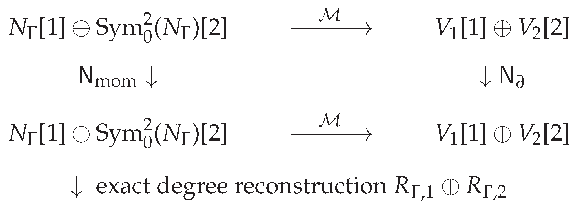
At this stage the carrier, carrier-group representation, family rank, and channel grading are fixed. The matrix elements of (138), the singular values of the direct blocks, the neutral Schur denominator, and the contact coefficients remain completed data. Their quantitative analysis is carried out in Section 5.

3.8. Primitive Graded Standard-Model Reconstruction Theorem

Theorem 4 

(Primitive graded Standard-Model reconstruction). Let Γ satisfy S1-S7 of Table 4. Then the minimal finite carrier is (56), with grading (60), taken modulo the Borel-Weil witness descent of Corollary 2. Under S8 and S9, its determinant-preserving carrier group is (64), its fixed chiral finite module is (69), and the canonical Abelian gradings are (70) and (72). The global form is (65). Under S10 and S11, the finite cocharacter shadow is (82) and its parity-selected module is (90). If the analytic hypotheses of Proposition 26 also hold, this module is attached as the rank-three factor (146) in each simple primitive low channel. The direct, Majorana, and contact channels are those of Table 8.

Proof. 

The carrier statement is Theorem 2. The carrier group follows from (63), and the Clifford and determinant statements follow from Proposition 10 and Proposition 12. The finite-shadow module follows from Proposition 14 and Proposition 16. The low attachment follows from Proposition 26 and Corollary 8. □

Remark 1 

(Structural carrier package). The carrier split, compact carrier group, one-generation Fock module, hypercharge, finite cocharacter kernel, and parity-selected three-dimensional module are successive readings of the integral grading reconstructed from the two active source orders.

Remark 2 

(Structural boundary-cycle package). The finite boundary-cycle package consists of the carrier (56), the determinant group (64), the Fock module (69), the finite shadow (86), and the Hodge-spectral torsor module (99). Its state-level consequences are given by (129), (130), and (133).

The Alena-Codazzi realization in the next section supplies a geometric source for S1-S3 and a conditional mechanism for the transported boundary data. The identification of the moment grading with the Borel-Weil level remains the exact reconstruction closure S6. The completed spectral and quantitative problem is treated after the realization layer has been fixed.

4. Alena-Codazzi Realization of the Reconstruction Data

The structural theorem of Section 3 starts from a primitive projective link, a degree-resolved two-channel normal source, relative Gauss-local charges, and admissible boundary transport. The present section gives an explicit compact-leaf source model and formulates a geometric realization criterion for these inputs. Within this criterion, a current-residual Alena-Codazzi collar supplies the compact-leaf source, the thin-core worldline component, the source Euler grading, and the two principal boundary charges. Torsor-admissible transport supplies the finite edge data required by the projective-color complex.

When the realization criterion is satisfied, the resulting collar fixes the source side of the reconstruction. The identification of the source Euler grading with the Borel-Weil level remains the exact degree closure of Definition 6. The determinant, Clifford, and finite-shadow constructions are then those of Section 3. The completed matrix elements are treated in Section 5.

4.1. Current-Codazzi Collar and Multiplier Closure

The residual part of the Alena-type current branch is written as

$${\mathcal{L}}_{\mathrm{cr}}=\phi p_{\Lambda },\phi =1-{\zeta }^2-{\mu }_{\zeta }{R}_{\omega }.$$

(147)

Here $\zeta$ is the translational-current amplitude, ${\mu }_{\zeta }={\mu }_{\zeta }({\rho }_{\zeta })$ is positive, and $R_{\omega }$ is the normalized vorticity response. The branch-stress interpretation is supplied by the Alena Tensor identification [65]. The current and vorticity slots are those of [66]. The continuum, variational, and branch-potential inputs are represented by [67,68,69]. Only the current, vorticity, stress, and Codazzi coefficients are used in the realization below.

The translational current is

$$J_{\mathrm{tr}}^{\mu }=p_{\Lambda }{\zeta }^2{U}^{\mu },{\nabla }_{\mu }^{(k)}{J}_{\mathrm{tr}}^{\mu }=0.$$

(148)

The frozen scalar block is assumed non-degenerate:

$$V_{\zeta }^{\prime \prime }({\rho }_{\zeta })+R_{\omega }{\mu }_{\zeta }^{\prime \prime }({\rho }_{\zeta })>0.$$

(149)

This condition gives local persistence of the scalar collar inside the selected current branch.

The product-rule Hilbert response of (147) is decomposed as

$$T_{\mu \nu }^{\mathrm{cr}}={\Xi }_{\mu \nu }+\phi Y_{\mu \nu }.$$

(150)

The first term records the response of the residual scalar density. The second carries the branch-response coefficient associated with $p_{\Lambda }$. The punctured collar is split-conserved when

$${\nabla }_{\mu }^{(k)}{\Xi }^{\mu \nu }=0,{\nabla }_{\mu }^{(k)}(\phi Y^{\mu \nu })=0.$$

(151)

The split is used before the normal two-jet is extracted.

Let $\tau =k^{\mu \nu }{Y}_{\mu \nu }$ and put

$$B_{\mu \nu }=Y_{\mu \nu }-{\displaystyle \frac{1}{3}}\tau k_{\mu \nu }.$$

(152)

The indices in this subsection range over the four-dimensional collar. The tensor B is the trace-adjusted branch coefficient used in the multiplier equation. Its trace-free principal normal projection supplies the order-two source coefficient below. A nonzero scalar $\phi$ is a Codazzi multiplier when

$$A_{\mu \nu }=\phi B_{\mu \nu }$$

(153)

satisfies the trace-adjusted Codazzi equation on the source-free collar. Define

$$C_{\alpha \mu \nu }^B={\nabla }_{\alpha }^{(k)}{B}_{\mu \nu }-{\nabla }_{\mu }^{(k)}{B}_{\alpha \nu },\theta =dlog|\phi |.$$

(154)

The multiplier equation is

$$C_{\alpha \mu \nu }^B+{\theta }_{\alpha }{B}_{\mu \nu }-{\theta }_{\mu }{B}_{\alpha \nu }=0.$$

(155)

On a connected open set where $B_{\mu \nu }$ is invertible, let ${\beta }^{\mu \nu }$ denote its inverse. Contraction of (155) determines

$${\theta }_{\alpha }^B=-{\displaystyle \frac{1}{3}}{\beta }^{\mu \nu }{C}_{\alpha \mu \nu }^B.$$

(156)

The coefficient $1/3$ in (156) is ${(dim\Omega -1)}^{-1}$ for the four-dimensional collar.

Proposition 27 

(Current-Codazzi closure). Let Ω be a connected source-free collar set on which $B_{\mu \nu }$ is invertible. A nonzero scalar Codazzi multiplier exists if and only if (155) holds with $\theta ={\theta }^B$ and ${\theta }^B$ is exact on Ω. If ${\theta }^B=d{f}_B$, then

$$\phi =C_{\phi }{e}^{f_B},{\zeta }^2=1-{\mu }_{\zeta }{R}_{\omega }-C_{\phi }{e}^{f_B},$$

(157)

where $C_{\phi }\ne 0$. The remaining current compatibility is

$$\begin{array}{cc}\hfill U({\mu }_{\zeta }{R}_{\omega })+C_{\phi }{e}^{f_B}{\theta }^B(U)=& \left(1-{\mu }_{\zeta }{R}_{\omega }-C_{\phi }{e}^{f_B}\right)\hfill \\ \hfill & \times \left({\nabla }_{\mu }^{(k)}{U}^{\mu }+U(log{p}_{\Lambda })\right).\hfill \end{array}$$

(158)

Proof. 

Substitution of (153) into the Codazzi equation gives (155). Its contraction with ${\beta }^{\mu \nu }$ gives (156). Exactness gives $\phi =C_{\phi }{e}^{f_B}$. Equation (157) follows from (147), and current conservation gives (158). □

The multiplier criterion is local on the connected non-degenerate collar. Global existence additionally requires the vanishing of the periods of ${\theta }^B$. The realization theorem below uses exact multiplier closure on the selected punctured collar.

4.2. Compact-leaf Source and Conditional Thin-Core Extraction

An explicit compact-leaf source model is supplied by a warped collar. Let ${\Sigma }_g$ be a compact hyperbolic surface of genus $g\ge 2$, with metric $\gamma$. On a frozen collar interval, let $s=tanh\chi \in (0,1)$ be the leaf anisotropy and let $a(s)>0$ be the warp factor. The two-eigenvalue Codazzi first integrals contain a constant $F_0$. The warped-product curvature convention is the one of [11].

The normalized vorticity closure has the leaf equation

$${\Delta }_{\gamma }\alpha ={\sigma }_{\omega }{\displaystyle \frac{2a{(s)}^2{D}_o^2}{c^{2}s}},{\sigma }_{\omega }=\pm 1,$$

(159)

where $D_o\ne 0$ is the frozen vorticity-flux scale. The right-hand side has nonzero mean. A one-core regularization is obtained by choosing a non-negative mollifier ${\rho }_{\epsilon }$ with unit integral and setting

$${\Delta }_{\gamma }{\alpha }_{\epsilon }={\sigma }_{\omega }{\displaystyle \frac{2a{(s)}^2{D}_o^2}{c^{2}s}}+q_{\epsilon }(s){\rho }_{\epsilon },$$

(160)

where

$$q_{\epsilon }(s)=-{\sigma }_{\omega }{\displaystyle \frac{2a{(s)}^2{D}_o^2}{c^{2}s}}{Area}_{\gamma }({\Sigma }_g).$$

(161)

The right-hand side of (160) has zero integral. The resulting compact Poisson problem is therefore solvable, uniquely after the additive constant has been fixed, by the standard elliptic result represented by [35]. If ${\rho }_{\epsilon }\rightharpoonup {\delta }_p$, the limit has one distributional leaf source at p. Transport of p along a timelike integral curve gives the local core.

Source-free will mean singular-source-free. The smooth zero-mode-compensating term in (160) is retained as part of the frozen leaf geometry. The principal boundary data are read after subtraction of a smooth local particular solution.

The same frozen sector has Codazzi gap

$${\Delta }_C=-{\displaystyle \frac{2F_0}{3-s}}.$$

(162)

For $F_0\ne 0$ and $0<s<1$, the collar lies in the non-degenerate two-eigenvalue sector used by the projective-link construction.

Proposition 28 

(Resolved compact-leaf source collar). Let ${\Sigma }_g$ be a compact hyperbolic leaf with $g\ge 2$. For every frozen range with $0<s<1$, $D_o\ne 0$, and $F_0\ne 0$, equation (160) has a unique smooth solution with zero mean. As ${\rho }_{\epsilon }\rightharpoonup {\delta }_p$, its source converges to a one-core distributional closure. Away from the core, after subtraction of the smooth background, the collar is singular-source-free and has the nonzero gap (162).

Proof. 

The zero-mean condition follows from (161). Compact elliptic solvability gives the smooth solution. Weak convergence of the mollifier gives the distributional limit, and the gap statement is immediate from (162). □

Smooth frozen-background terms do not alter the finite carrier when the singular associated-graded charges, their source grading, and the nonzero gap are unchanged. The support selection depends on the primitive link and the degree-resolved non-scalar source.

The compact-leaf model is compatible with the current-residual scalar under the following local condition.

Proposition 29 

(Compatibility with the current-residual form). Let Ω be a connected non-degenerate punctured collar on which $B_{\mu \nu }$ is invertible. Assume that a smooth nonzero scalar ${\varphi }_C$ makes ${\varphi }_C{B}_{\mu \nu }$ trace-adjusted Codazzi. Let $p_{\Lambda }>0$ and let U be smooth. Suppose that positive initial data may be chosen for

$$U(y)+y\left({\nabla }_{\mu }^{(k)}{U}^{\mu }+U(log{p}_{\Lambda })\right)=0$$

(163)

so that its solution satisfies $1-{\varphi }_C-y={\mu }_{\zeta }{R}_{\omega }$ with the required sign. After restriction to a smaller flow collar if required, the calibrated tensor has the representation

$${\varphi }_C=1-{\zeta }^2-{\mu }_{\zeta }{R}_{\omega },{\zeta }^2>0,{\nabla }_{\mu }^{(k)}\left(p_{\Lambda }{\zeta }^2{U}^{\mu }\right)=0.$$

(164)

Moreover, ${\varphi }_C=C_{\varphi }{e}^{f_B}$ and ${\theta }^B=d{f}_B$.

Proof. 

Proposition 27 gives

$${\theta }^B=dlog|{\varphi }_C|.$$

(165)

Thus ${\varphi }_C=C_{\varphi }{e}^{f_B}$. Positive initial data for (163) remain positive along the U-flow. With $y={\zeta }^2$, define

$${\mu }_{\zeta }{R}_{\omega }=1-C_{\varphi }{e}^{f_B}-y.$$

(166)

Equations (163) and (166) give (164) and (158). □

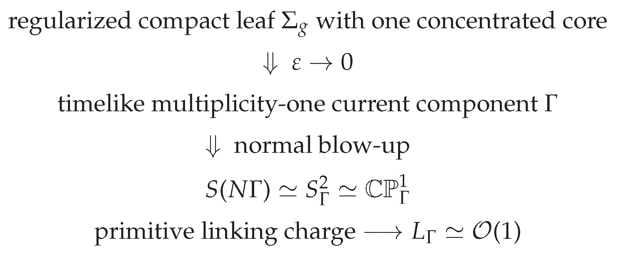
Under the regularity hypothesis stated below, the thin-core limit identifies the primitive worldline component. The compactness input is supplied by integral-current compactness [70], in the geometric-measure form represented by [71]. Vortex concentration gives the comparison with [72]; the Jacobian-current formulation is represented by [73]. A smooth auxiliary Riemannian metric h is fixed on the collar. All mass bounds and local flat compactness statements below are taken with respect to h, while timelikeness and orthogonal normal bundles are defined by the Lorentzian metric.

Theorem 5 

(Conditional thin-core extraction). Let $\{{\mathcal{C}}_{\epsilon }\}$ be regularized Alena-Codazzi collars and let $T_{\epsilon }$ be the integral 1-current carried by their regularized cores. Assume:

(i)

the local masses of $T_{\epsilon }$ and $\partial T_{\epsilon }$ are uniformly bounded;

(ii)

$\partial T_{\epsilon }=0$ on the singular-source-free part of the collar;

(iii)

the integral linking charge converges to a primitive degree-one charge;

(iv)

the trace-adjusted Codazzi residual converges to zero in $H_{\mathrm{loc}}^{-1}$ away from every subsequential current limit;

(v)

the absolute frozen Codazzi gap is uniformly bounded below on compact subsets disjoint from the cores;

(vi)

the component selected by the primitive linking charge is a regular timelike multiplicity-one component of the limiting current.

After passage to a subsequence, $T_{\epsilon }$ converges locally to an integral 1-current T without interior boundary on the source-free collar. The selected regular component is a timelike worldline Γ. Its oriented normal bundle gives (41), and the limiting charge gives (44). The trace-adjusted Codazzi equation holds distributionally away from $sptT$.

Proof. 

Integral-current compactness gives a locally convergent subsequence. Boundary continuity gives the absence of interior boundary. The residual convergence gives the distributional Codazzi equation away from the limit. The selected regular multiplicity-one component is represented by a timelike worldline. The limiting primitive charge gives (44), and the uniform gap supplies the two-eigenvalue splitting on the punctured collar. □

Figure 1. Compact-leaf concentration, the thin-core worldline, and the resolved projective link.

Figure 1. Compact-leaf concentration, the thin-core worldline, and the resolved projective link.

4.3. Moment-Resolved Source and Preservation of the Euler Grading

Let $N_{\Gamma }$ be the oriented transverse normal fiber. A second-order normal source has a first moment $m\in N_{\Gamma }$ and a trace-free second moment $M_0\in {Sym}_0^2(N_{\Gamma })$. The scalar trace belongs to the singlet channel and is separated before the finite support problem.

Definition 10 

(Second-order moment-resolved source). A defect source is second-order moment-resolved when its associated-graded scalar-sector source up to transverse order two is represented in defect-adapted normal coordinates by a normalized core profile with first moment m and trace-free second moment $M_0$, and when the singular degree-two coefficient of the harmonic potential of its principal trace-free Codazzi representative is ${\kappa }_2{M}_0$ for a fixed $0\ne {\kappa }_2\in \mathbb{R}$.

For $\omega \in S(N_{\Gamma })$, the non-scalar link map is

$$\mathcal{M}:N_{\Gamma }\oplus {Sym}_0^2(N_{\Gamma })⟶V_1\oplus V_2,\mathcal{M}(m,M_0)=\left(m·\omega ,{\omega }^T{M}_0\omega \right).$$

(167)

This is the equivariant identification of oriented normal vectors with degree-one spherical harmonics and trace-free quadratic forms with degree-two spherical harmonics.

Let ${\mathsf{N}}_{\mathrm{mom}}$ act with eigenvalue 1 on $N_{\Gamma }$ and eigenvalue 2 on ${Sym}_0^2(N_{\Gamma })$. Then

$$\mathcal{M}\circ {\mathsf{N}}_{\mathrm{mom}}={\mathsf{N}}_{\partial }\circ \mathcal{M}.$$

(168)

Thus the moment map preserves the source Euler grading. Frozen normal transport preserves the same homogeneous degree on a source-free annulus. The two-channel locus $m\ne 0$, $M_0\ne 0$ is open and dense in the finite moment space.

A prescribed trace-free second moment is compatible with a positive core profile. A sufficiently large scalar trace may be added to the raw second moment; this changes only the separated scalar channel.

The associated non-scalar two-jet is

$${\left(gr{J}_{\perp }^{\le 2}\right)}_{\mathrm{ns}}=\mathcal{M}(m,M_0)\in V_1[1]\oplus V_2[2].$$

(169)

Equation (168) supplies the source-side grading required by S2 of Table 4. Its identification with the section-space level is imposed by (55).

Figure 2. Preservation of the source Euler grading by the moment-resolved link map.

Figure 2. Preservation of the source Euler grading by the moment-resolved link map.

4.4. Gauss-local Charges and Transported Boundary Data

Let $j_{\mathrm{tr}}^i$ be the principal normal reduction of (148). Extend the first moment m in the frozen normal frame by ${\nabla }^{\perp }m=0$ and put ${\mathbf{j}}_1^i=m{j}_{\mathrm{tr}}^i$. Let $A_{ij}$ be the trace-free principal Codazzi representative.

Lemma 6 

(Principal current and Codazzi-Gauss charges). On a source-free principal normal annulus, ${\nabla }_i^{\perp }{\mathbf{j}}_1^i=0$. The $V_1$ current-flux charge is

$$Q_1(r)={\int }_{S_r^2}{\mathbf{j}}_1^i{n}_{i}dS\in N_{\Gamma }\simeq V_1.$$

(170)

Writing $q_{\mathrm{tr}}(r)={\int }_{S_r^2}{j}_{\mathrm{tr}}^i{n}_{i}dS$, one has $Q_1(r)=m{q}_{\mathrm{tr}}(r)$ and

$$Q_1(r_1)-Q_1(r_0)={\int }_{{\Omega }_{r_0,r_1}}{\nabla }_i^{\perp }{\mathbf{j}}_1^{i}dV=0.$$

(171)

The trace-free Codazzi representative has a harmonic Hessian potential,

$$A_{ij}={\partial }_i{\partial }_{j}u,\Delta u=0.$$

(172)

For $M\in {Sym}_0^2(N_{\Gamma })$, let $H_M(x)=M_{ij}{x}^i{x}^j$. The $V_2$ charge is determined by

$$〈Q_2(r),M〉={\int }_{S_r^2}\left(u{\partial }_n{H}_M-H_M{\partial }_{n}u\right)dS.$$

(173)

It is independent of r, and $Q_2=0$ if and only if $M_0=0$.

Proof. 

The principal current equation gives ${\partial }_i{j}_{\mathrm{tr}}^i=0$. Parallelity of m gives ${\nabla }_i^{\perp }{\mathbf{j}}_1^i=0$, and Stokes’ theorem gives (171).

For fixed k, the principal Codazzi equation makes $A_{ik}d{x}^i$ closed. Since $H^1({\mathbb{R}}^3\setminus \{0\})=0$, one obtains $A_{ik}={\partial }_i{v}_k$. Symmetry gives $v_k={\partial }_{k}u$, and trace-freeness gives $\Delta u=0$. Green’s identity gives the radius independence of (173). By Definition 10, the singular degree-two coefficient is ${\kappa }_2{M}_0$ with ${\kappa }_2\ne 0$, and the pairing on this term is a non-degenerate multiple of the standard $V_2$ inner product. □

The first moment is computed with origin on the regular component selected by Theorem 5. A normal translation which changes this component changes the defect datum. On the locus $q_{\mathrm{tr}}\ne 0$, the two charges are nonzero exactly when $m\ne 0$ and $M_0\ne 0$.

On a curved collar, $Q_1$ is compared by normal parallel transport. The $V_2$ charge is compared by the Green identity for the first-order Codazzi operator $\mathfrak{C}$ and its formal adjoint:

$${\int }_{{\Omega }_{r_0,r_1}}\left(\langle \mathfrak{C}A,\Psi \rangle -\langle A,{\mathfrak{C}}^{*}\Psi \rangle \right)={\mathcal{B}}_{S_{r_1}}(A,\Psi )-{\mathcal{B}}_{S_{r_0}}(A,\Psi ).$$

(174)

If $\mathfrak{C}A=0$ and ${\mathfrak{C}}^{*}\Psi =0$, the boundary pairing is independent of the linking radius. The transported current law is ${\mathsf{P}}_{r_0\leftarrow r_1}^{\perp }{Q}_1(r_1)=Q_1(r_0)$.

The fixed charge pair generates the boundary-charge algebra used in Definition 4. Lemma 3 then gives central type projections in every finite sector representation. Thus the current flux realizes the $V_1$ sector and the Codazzi-Gauss pairing realizes the $V_2$ sector.

4.5. Torsor-admissible Transport and Spectral Admissibility

The charge pair must be transported compatibly with the affine finite shadow before the torsor complex of (97) is obtained. This is an additional boundary condition on the realized source data.

Definition 11 

(Torsor-compatible boundary transport). An Alena-Codazzi collar is torsor-admissible when:

(i)

the $V_1$ charge (170) has a compact unitary phase calibration on linking spheres;

(ii)

the $V_2$ charge (173) is represented in a transported unitary Green-adjoint frame;

(iii)

the transported order-three normal-frame action is identified with the translation in (95);

(iv)

the relative charge transport descends to the unitaries $U_a$ in (98);

(v)

its completed low compression is compatible with (122);

(vi)

the edge transport and the low-high coupling are subcritical with respect to the separating Callias-Schur gap.

The transport is torsor-compatible when (102) vanishes. The flat subbranch additionally satisfies (103).

The first two entries fix unitary boundary normalizations. The third and fourth give the finite edge descent. The fifth controls the Schur-visible low symbol. Centrality of the Wilson defect gives a well-defined structural torsor cycle; its value remains a finite holonomy datum.

For torsor-admissible data, (171) and (174) induce the transports in (98). The scalar and mixed responses are then those of (105) and (118). The structural closure fixes centrality, while flatness selects the subbranch (103).

The analytic attachment requires a boundary-admissible normal representative with an isolated primitive cluster. The spectral projection is defined by a Riesz contour and persists under perturbations smaller than the spectral separation, in the standard sense of [8]. The open normal problem is compared with the Callias mechanism [9]; its geometric Fredholm form is represented by [10].

The primitive linking degree is locally constant under deformations which preserve the resolved transverse frame. The conditions $m\ne 0$ and $M_0\ne 0$ are open in the finite moment space. A nonzero Codazzi gap remains nonzero on a fixed compact subcollar under sufficiently small constrained perturbations. If the low-high coupling has norm below one half of the Callias-Schur separation, the rank of the isolated low projection remains fixed.

Persistence is taken inside the current-Codazzi class. An unrestricted neighborhood theorem for the multiplier would require solvability of the nonlinear map $(\phi ,B)\mapsto C(\phi B)$ together with the period condition for (156). Torsor admissibility remains a finite boundary-transport condition.

4.6. Alena-Codazzi Realization Theorem

Definition 12 

(Primitive Alena-Codazzi realization class). A current-residual Alena-Codazzi collar belongs to the primitive realization class when:

(i)

(147), (148), and (149) hold;

(ii)

the split conservation law (151) holds on the punctured collar;

(iii)

the residual scalar satisfies Proposition 27;

(iv)

the compact-leaf source has a nonzero frozen gap and a one-core thin limit;

(v)

the selected thin-core component is timelike, regular, multiplicity one, and carries the primitive linking charge;

(vi)

the moment pair satisfies $m\ne 0$, $M_0\ne 0$, and $q_{\mathrm{tr}}\ne 0$;

lgbel=()

the local algebra is relative Gauss-local with the charge pair fixed on the boundary.

It is Schur-admissible when the selected normal representative has an open Callias-Schur gap and subcritical low-high coupling, and when the normal family and its low-high coupling are basic under admissible reconstruction-frame transitions.

The relation between the assumptions of Section 3 and the present realization is summarized in Table 10.

Theorem 6 

(Alena-Codazzi realization of the primitive graded defect). Let $\{{\mathcal{C}}_{\epsilon }\}$ be a family of collars satisfying:

(i)

current-Codazzi closure in the sense of Proposition 27;

(ii)

the compact-leaf source construction of Proposition 28;

(iii)

the current-residual compatibility of Proposition 29;

(iv)

the thin-core hypotheses of Theorem 5;

(v)

a moment-resolved source with $m\ne 0$, $M_0\ne 0$, and $q_{\mathrm{tr}}\ne 0$;

(vi)

a relative Gauss-local algebra with the two boundary charges fixed.

The limiting collar supplies a primitive graded defect datum in the sense of Definition 5. Its source Euler grading is preserved by (168). After closure of S4-S7 in Table 4, the minimal finite support is (56). If the collar is Schur-admissible, the selected support is represented by an isolated low bundle on the protected quotient. Its rank, projected connection, and reduced normal penalty persist under the stated gap condition.

Proof. 

The current-Codazzi scalar and the exact multiplier are supplied by Proposition 27. The compact-leaf construction gives a source model with nonzero frozen gap, while Proposition 29 gives the current-residual representative.

Theorem 5 identifies the selected regular component with the limiting timelike worldline and supplies its projective link and primitive line. The nonzero moment pair gives (169), and (168) preserves its normal order. Lemma 6 gives the two nonzero charges and their invariance on the source-free annulus. Relative Gauss locality supplies their central sector labels. These are the data of Definition 5. The support statement follows from Theorem 2. Spectral persistence follows from the Callias-Schur separation. □

Corollary 9 

(Realization of the finite boundary transport). Assume the hypotheses of Theorem 6 and let the limiting collar be torsor-admissible. Then its transported charge pair supplies the edge transports of (98). Closure of (102) realizes the projective-color Hodge-spectral module (99) on the boundary data. The flat subbranch is selected by (103).

Proof. 

The $V_1$ transport follows from (171) and the normal connection. The $V_2$ transport follows from (174). Definition 11 gives their descent to the finite edge transports. Closure of (102) places the Wilson element in $Z({\mathfrak{A}}_{\Gamma }^{\mathrm{tr}})$. □

The geometric realization therefore supplies the primitive link, the two graded source channels, their Gauss-local boundary charges, and the admissible finite transport. Exact degree fidelity and the remaining finite closures are applied to these realized data through Theorem 4. The completed direct, neutral, and contact branches are evaluated on the resulting boundary cycle.

5. Schur Completion, Quantitative Branches, and Falsification

The primitive graded carrier, the determinant-compatible Fock module, the finite cocharacter shadow, and the conditional rank-three low factor have been fixed in Section 3. Section 4 supplies their current-Codazzi realization data. The present section treats the completed low operator on this boundary cycle. The direct, neutral, scalar, and contact entries are organized by the $B-L$ and exterior-bidegree filtration of Table 8.

The completed layer has three distinct statuses. Matrix elements and Schur denominators are branch data. Scale-free residuals test the shape of a chosen branch. Numerical values are reported only after the primitive normalization, path multiplicities, Pfaffian reading, or threshold prescription required by the corresponding entry has been fixed. None of these completed readings is used in the carrier theorem.

5.1. Completed Low Operator and Schur No-Phantom Reduction

The low operator is the locked finite operator of (138), acting on the isolated module supplied by Proposition 26. It is taken after the structural witness descent and the penalty reduction of Lemma 1. The projected connection is (136), and the first high-sector correction is the Schur compression (140). Higher integer moments enter with the suppression stated in Proposition 25. The structural channel classes have already been fixed in Table 8. Mass readings in the completed branch are extracted from singular values, spectral gaps, or finite Hessians of the reduced operator.

The finite Yukawa blocks are compressed matrix elements of the zero-order part of the locked operator:

$${(Y_{AB})}_{ij}=〈{\psi }_i^A,P_{\mathrm{low}}\left(c(\Phi +{\Phi }^{†})+Q_{\mathrm{hol}}+Q_C\right)P_{\mathrm{low}}{\psi }_j^B〉.$$

(175)

The exterior package fixes the possible pairs $(A,B)$; the entries in (175) are completed-branch data. In a local orthonormal low-mode frame, (136) has matrix coefficients $A_{ij}=\langle {\psi }_i,d{\psi }_j\rangle$. These are the projected gauge coefficients of the selected carrier. The determinant reduction of the projected connection is the projection to (81).

After the central factor (96) has been isolated, each direct Hermitian family block $H_f=Y_f{Y}_f^{†}$ has a Schur-visible first family-motion part $H_f^{(1)}$. Its finite Hodge-Schur bookkeeping is

$$H_f^{(1)}=H_f^{\mathrm{circ}}+{\Gamma }_f,{\Gamma }_f={\Pi }_{\mathrm{noncirc}}(H_f^{(1)}).$$

(176)

Here $H_f^{\mathrm{circ}}$ is the circulant part, while $H_f-H_f^{(1)}$ contains higher Schur terms not used in the first family-motion test. The projection is the one in (116). Thus only ${\Gamma }_f$ is tested by the mixed torsor curvature (118) at first order.

The completed branch is represented by a finite Schur-Kuranishi map. After gauge, diffeomorphism, and unitary redundancies have been removed, let b denote the remaining branch coordinates and put

$${\mathcal{F}}_{\mathrm{fin}}(b)=P_{\mathrm{obs}}\left(K_{\mathrm{eff}}(b)\right),{\mathcal{F}}_{\mathrm{fin}}(b)=0.$$

(177)

Here $P_{\mathrm{obs}}$ denotes the projection to the finite observable obstruction coordinates of the completed low branch. Different sectors of ${\mathcal{F}}_{\mathrm{fin}}$ are filtered by $B-L$ and by exterior bidegree. The completed protected interface is

$${\mathcal{P}}_{\mathrm{Sch}}(b)=\left(j_b^{r_{\mathrm{Sch}}}{\mathcal{F}}_{\mathrm{fin}},{\mathcal{M}}_{\mathrm{pre}-\mathrm{Schur}},[P_{\mathrm{low}}(b),{\nabla }_{\mathrm{low}}(b)],{\Delta }_{\mathrm{low}}(b)\right),$$

(178)

where $j_b^{r_{\mathrm{Sch}}}{\mathcal{F}}_{\mathrm{fin}}$ is the jet retained by the chosen Schur order, ${\mathcal{M}}_{\mathrm{pre}-\mathrm{Schur}}$ collects the boundary-sector projections, the $B-L$ and exterior-bidegree filtrations, and the finite-shadow and torsor labels, and $[P_{\mathrm{low}},{\nabla }_{\mathrm{low}}]$ denotes the marking-preserving unitary class of the isolated low bundle with its projected connection. The scalar ${\Delta }_{\mathrm{low}}$ is the isolating Riesz gap.

Definition 13 

(Schur-phantom channel). Let $b=b_{\mathrm{red}}\oplus x$ be a local split of the finite branch coordinates in (177), after gauge, diffeomorphism, unitary, and structural witness redundancies have been removed. The finite coordinate channel x is called Schur-phantom at b when ${\mathcal{P}}_{\mathrm{Sch}}(b_{\mathrm{red}}\oplus x)\simeq {\mathcal{P}}_{\mathrm{Sch}}(b_{\mathrm{red}})$ to the retained Schur order. The channel is removable when the deletion $x\mapsto 0$ strictly lowers a monotone finite Schur-coordinate complexity ${\mathcal{C}}_{\mathrm{Sch}}$.

Proposition 30 

(Schur no-phantom reduction). Let b be a local zero of (177) in a fixed reconstruction class, after the entries preceding ${\mathfrak{E}}_{\mathrm{Schur}}$ in (12) have been closed. Let the retained finite Schur representative be observable-generated to the retained order. If x is a removable Schur-phantom channel in the sense of Definition 13, then $x=0$ in the finite reconstruction core, and its deletion strictly lowers ${\mathcal{C}}_{\mathrm{Sch}}$.

Proof. 

The protected interface (178) is unchanged by the deletion. Proposition 2 therefore applies with complexity ${\mathcal{C}}_{\mathrm{Sch}}$. □

Thus Definition 13 is the completed-layer specialization of protected-output descent. A completed numerical correction belongs to the reduced branch only if it changes (178) or is retained through the gap-mediated Schur compression (140). The higher-moment terms of Proposition 25 are of the latter type.

Figure 3. Completed Schur architecture on the structurally fixed low carrier.

Figure 3. Completed Schur architecture on the structurally fixed low carrier.

The reduced completed branch contains every channel forced by the retained observables, the finite filtration, or the gap-mediated compression. A coordinate invisible to these data is removed by Proposition 30.

5.2. Direct Dirac Sector, CKM Motion, and Charged-Lepton Balance

5.2.1. Non-circulant Direct-Family Motion

The projective-color carrier and its mixed-curvature detector were fixed in SubSection 3.6. A common circulant baseline is diagonalized by the finite Fourier basis. Physical quark mixing is therefore measured by the relative non-circulant motion of the up- and down-type direct blocks.

The CKM matrix is generated by a non-circulant component of the completed low operator. Let $N_{+}$ denote the positive normal representative, let $P_b$ be its isolated low projection, and put $Q_b=\mathbf{1}-P_b$. For a branch parameter X, the Schur-visible detector is

$$V_X=Q_b({\partial }_X{N}_{+})P_b.$$

(179)

The inverse Sylvester map transfers such a component to the motion of the low projection and hence to the finite Berry-Wilczek-Zee connection [62]. For two branch directions $X,Y$, the curvature of the projected low bundle is read in the standard projected form

$${\Omega }_{XY}^{\mathrm{BWZ}}=P_b[{\partial }_X{P}_b,{\partial }_Y{P}_b]P_b.$$

(180)

Thus a Schur-visible detector contributes to family mixing through the induced motion of the isolated low projection. By Proposition 21, the finite test for this central part is the non-circulant projection (116). Relative $V_1/V_2$ charge transport supplies such a source when its low symbol in (122) is nonzero and has degree one or two.

A CP-sensitive central invariant is obtained after the two direct Dirac sectors have been compared. Let ${\Gamma }_u$ and ${\Gamma }_d$ denote the first non-circulant Schur-visible Hermitian corrections in the up and down blocks, after the common circulant baseline has been removed. The finite CP-odd diagnostic is

$$J_{\mathrm{cen}}=\Im Tr\left({[{\Gamma }_u,{\Gamma }_d]}^3\right).$$

(181)

It vanishes when the two corrections are contained in a common commuting family algebra. The normalization relating (181) to the physical quark invariant is a completed Schur-Berry datum, with the standard comparison convention given by [74].

A minimal Hermitian non-circulant detector pair is represented by the clock-sine and shifted edge operators. The completed Schur-Berry edge phase is denoted by ${\vartheta }_{\Gamma }$; in a one-phase lift it is identified with the torsor edge phase of (98), subject to the finite-shadow coherence (92). Put

$$K_Z={\displaystyle \frac{Z-Z^{†}}{2i}},H_S({\vartheta }_{\Gamma })=e^{-i{\vartheta }_{\Gamma }}S+e^{i{\vartheta }_{\Gamma }}{S}^{†}.$$

(182)

Their finite central loop has the invariant

$${\mathcal{J}}_{\mathrm{cen}}({\vartheta }_{\Gamma })=\Im Tr\left({[K_Z,H_S({\vartheta }_{\Gamma })]}^3\right)={\displaystyle \frac{9\sqrt{3}}{2}}sin(3{\vartheta }_{\Gamma }).$$

(183)

Thus the invariant depends on the total phase around the central three-cycle. In the one-phase direct-Dirac reduction, the CP-sensitive closure is

$$J_q=s_{12}{s}_{23}{s}_{13}{c}_{12}{c}_{23}{c}_{13}^{2}sin(3{\vartheta }_{\Gamma }).$$

(184)

Here $3{\vartheta }_{\Gamma }$ is the rephasing-invariant CKM phase in the one-phase reduction. The condition fixes the completed loop phase after the three CKM magnitudes and the quark Jarlskog invariant have been specified. The carrier, torsor complex, and non-circulant detector remain fixed under this phase closure. The one-phase reduction uses the central torsor closure (102); flatness is the separate subbranch (103).

Proposition 31 

(Central spectral-CP identity). Assume the scalar one-phase lift, with ${\theta }_{\Gamma }={\vartheta }_{\Gamma }$ and cycle-trivial coefficient transport. Then

$${Disc}_{\mu }{\chi }_{{\Delta }_{\theta }}=108{sin}^2(3{\vartheta }_{\Gamma })={\displaystyle \frac{16}{9}}{\mathcal{J}}_{\mathrm{cen}}{({\vartheta }_{\Gamma })}^2.$$

(185)

Consequently, the central CP loop is nonzero precisely when the scalar torsor spectrum is simple.

Proof. 

Under the stated lift, (101) gives $w_{\Gamma }=4{sin}^2(3{\vartheta }_{\Gamma }/2)$. Substitution in (113), followed by (183), gives (185). □

A Schur-visible central detector contained in $\mathbb{C}[S]$ is simultaneously diagonalized with the circulant family baseline and has vanishing nonabelian family curvature; equivalently, (116) vanishes in that subcase. A detector pair containing the two degrees in (182) has nonzero commutator for generic ${\vartheta }_{\Gamma }$ and gives the central loop invariant (183). Relative $V_1/V_2$ charge transport supplies such a clock degree when its Schur-visible low symbol has a nonzero component in ${\mathcal{A}}_1\oplus {\mathcal{A}}_2$.

Let $H_f^{(0)}$ be the leading circulant Hermitian family block in a direct Dirac sector and let ${\Gamma }_f$ be the first non-circulant Schur-visible correction. In the Fourier basis of $H_f^{(0)}$, the first basis change is

$${({\Theta }_f)}_{ij}={\displaystyle \frac{{({\Gamma }_f)}_{ij}}{h_{f,j}^{(0)}-h_{f,i}^{(0)}}},i\ne j,{({\Theta }_f)}_{ii}=0.$$

(186)

Thus

$$V_{\mathrm{CKM}}=1+{\Theta }_d-{\Theta }_u+O({\Gamma }^2).$$

(187)

The standard CKM conventions are those of [75,76,77]. The CP-sensitive normalization is the one associated with (181).

Proposition 32 

(Direct Dirac CKM mechanism). Assume that the leading up- and down-type Hermitian family blocks belong to the same circulant algebra $\mathbb{C}[S]$ and have simple spectra. Then, in the common Fourier phase convention, CKM mixing is generated to first order by the relative non-circulant Schur-visible corrections to the two blocks. It is given by (187), and the finite test for the relevant correction is (118).

Proof. 

The leading circulant blocks have a common Fourier basis. A circulant correction remains diagonal in that basis and gives no off-diagonal term in (186). Hence only the non-circulant part of the Schur-visible correction contributes to the first basis motion. Proposition 21 identifies this part with the mixed torsor curvature norm (118). Taking the relative basis change between the down and up sectors gives (187). □

Corollary 10 

(CKM torsor-curvature bound). Assume that the leading circulant Hermitian blocks in the up and down direct Dirac sectors have simple spectra. Let ${\delta }_f={min}_{i\ne j}|h_{f,j}^{(0)}-h_{f,i}^{(0)}|$ for $f=u,d$, and let ${\parallel ·\parallel }_{\mathrm{F}}$ be the Frobenius norm on the central block. Then the first-order CKM displacement satisfies

$$\parallel V_{\mathrm{CKM}}{-\mathbf{1}\parallel }_{\mathrm{F}}\le {\displaystyle \frac{1}{\sqrt{3}}}\left({\displaystyle \frac{\parallel [d_{\theta },{\Gamma }_d]{\parallel }_{\mathrm{F}}}{{\delta }_d}}+{\displaystyle \frac{\parallel [d_{\theta },{\Gamma }_u]{\parallel }_{\mathrm{F}}}{{\delta }_u}}\right)+O_{{\delta }_u,{\delta }_d}\left((\parallel {\Gamma }_u{\parallel }_{\mathrm{F}}+\parallel {\Gamma }_d{{\parallel }_{\mathrm{F}})}^2\right).$$

(188)

Proof. 

Equation (186) gives the first-order basis motion with denominators bounded below by ${\delta }_f$. Taking the Frobenius norm in (187) gives the corresponding sum of up and down contributions. The identity (118) gives $\parallel {\Pi }_{\mathrm{noncirc}}{\Gamma }_f{\parallel }_{\mathrm{F}}=3^{-1/2}{\parallel [d_{\theta },{\Gamma }_f]\parallel }_{\mathrm{F}}$ for the uniform-phase torsor differential (104). The second-order remainder is controlled by the same simple-spectrum gaps. Substitution gives (188). □

Definition 14 

(Minimal non-circulant Hodge-Schur direct branch). After the carrier, finite shadow, projective-color torsor, and $B-L$ filtration have been fixed, let ${\mathcal{P}}_{\mathrm{dir}}$ be a reduced source-generated class of Schur-visible direct paths, including their valuations and path multiplicities. A direct quark branch is called minimal non-circulant Hodge-Schur relative to ${\mathcal{P}}_{\mathrm{dir}}$ if the common circulant baseline is removed as in (176), the branch is non-flat in the seminorm (119), and, at fixed nonzero direct-block normalization $\parallel {\Gamma }_u{\parallel }_{\mathrm{F}}^2+{\parallel {\Gamma }_d\parallel }_{\mathrm{F}}^2={\Lambda }_{\mathrm{dir}}^2$, the relative up-down correction minimizes the residual

$${\mathcal{K}}_{\mathrm{HS}}(u,d)={\displaystyle \frac{{\mathcal{L}}_{\Gamma }{({\Gamma }_d)}^2}{{\delta }_d^2}}+{\displaystyle \frac{{\mathcal{L}}_{\Gamma }{({\Gamma }_u)}^2}{{\delta }_u^2}}$$

(189)

among corrections supported on ${\mathcal{P}}_{\mathrm{dir}}$ whose relative $V_1/V_2$ low symbol has a nonzero component in ${\mathcal{A}}_1\oplus {\mathcal{A}}_2$. Here ${\delta }_f$ is the direct-sector gap used in Corollary 10, while ${\Lambda }_{\mathrm{dir}}>0$ is completed-branch data expressed in the primitive units of Remark 3. Reduced closure excludes an independent lower-valuation direct $1\leftrightarrow 3$ edge when it is not sourced by the fixed Gauss-local data.

The definition is used only after the structural entries of Table 1 have been fixed. The class ${\mathcal{P}}_{\mathrm{dir}}$ belongs to the completed path data and is not selected by (189). On the non-circulant correction space, (118) gives ${\mathcal{L}}_{\Gamma }{({\Gamma }_f)}^2=3{\parallel {\Gamma }_f\parallel }_{\mathrm{F}}^2$. The residual therefore weights the admissible amplitudes by the direct gaps without distinguishing Weyl directions carrying the same path data. The fixed direct-block normalization prevents continuous rescaling from replacing the minimum by the zero infimum, and the least gap-weighted representative is selected within ${\mathcal{P}}_{\mathrm{dir}}$.

For the first family-motion block in (176), let

$${\rho }_f(\beta )={\displaystyle \frac{e^{-\beta H_f^{(1)}}}{{Tr}_{\mathrm{cen}}(e^{-\beta H_f^{(1)}})}},{\mathcal{C}}_f(\beta )={\mathcal{C}}_{\Gamma }({\rho }_f(\beta )),$$

(190)

where $\beta >0$ is a spectral probe parameter.

Proposition 33 

(Entropic family susceptibility). For $\beta \to 0$,

$${\mathcal{C}}_f(\beta )={\displaystyle \frac{{\beta }^2}{18}}{\mathcal{L}}_{\Gamma }{({\Gamma }_f)}^2+O({\beta }^3\parallel H_f^{(1)}{\parallel }_{\mathrm{F}}^3).$$

(191)

Consequently, the entropic susceptibility

$${\mathcal{X}}_f^{\mathrm{ent}}:=\underset{\beta \downarrow 0}{lim}{\displaystyle \frac{\sqrt{{\mathcal{C}}_f(\beta )}}{\beta }}={\displaystyle \frac{1}{3\sqrt{2}}}{\mathcal{L}}_{\Gamma }({\Gamma }_f)$$

(192)

exists, and (188) becomes

$$\parallel V_{\mathrm{CKM}}{-\mathbf{1}\parallel }_{\mathrm{F}}\le \sqrt{6}\left({\displaystyle \frac{{\mathcal{X}}_d^{\mathrm{ent}}}{{\delta }_d}}+{\displaystyle \frac{{\mathcal{X}}_u^{\mathrm{ent}}}{{\delta }_u}}\right)+O_{{\delta }_u,{\delta }_d}\left((\parallel {\Gamma }_u{\parallel }_{\mathrm{F}}+\parallel {\Gamma }_d{{\parallel }_{\mathrm{F}})}^2\right).$$

(193)

Moreover,

$${\mathcal{K}}_{\mathrm{HS}}(u,d)=18\left({\displaystyle \frac{{({\mathcal{X}}_d^{\mathrm{ent}})}^2}{{\delta }_d^2}}+{\displaystyle \frac{{({\mathcal{X}}_u^{\mathrm{ent}})}^2}{{\delta }_u^2}}\right).$$

(194)

Proof. 

At $\beta =0$, the state in (190) is $\mathbf{1}/3$, and its first non-circulant variation is $-\beta {\Gamma }_f/3$. Equation (191) follows from (129). Equations (192)-(194) follow from (119), (188), and (189). □

Thus the minimal non-circulant Hodge-Schur branch minimizes the weighted entropic susceptibility within the fixed source-generated class ${\mathcal{P}}_{\mathrm{dir}}$. Entanglement-based flavor selection in scattering gives an independent comparison [78]; here the entropy is fixed by the projective-color expectation (126), while the admissible Weyl directions and their valuations are fixed before the gap-weighted minimization.

The determinant-shadow scale used in SubSection 5.5 supplies the primitive path unit of this direct-branch diagnostic. The Cabibbo entry is carried by the primitive path, while the remaining quark magnitudes are read from the longer reduced paths and their Hilbert-Schmidt multiplicities. The loop CP datum is fixed separately by the central holonomy. These readings belong to the completed minimal branch; the carrier, torsor complex, and detector remain those of (118).

5.2.2. Charged-lepton Hodge Balance

The charged-lepton block is the color-singlet direct channel $L_L\leftrightarrow e_L^c$ in Table 8. Its scale-free shape is read on the three-sector torsor independently of the quark relative-basis problem and of the neutral Majorana denominator.

Let $x_{\ell }$ denote the positive charged-lepton amplitude vector on the three-sector torsor carrier,

$$x_{\ell ,r}=\sqrt{m_{\ell ,r}},r\in {\mathbb{Z}}_3.$$

(195)

The real regular projective-color representation decomposes into its invariant line and its orthogonal real two-dimensional torsor complement. The corresponding projections are $P_{\mathbf{1}}=(\mathbf{1}+S+S^2)/3$ and $P_{\mathrm{T}}=\mathbf{1}-P_{\mathbf{1}}$. Both commute with (105). In the reference normalization ${\theta }_{\Gamma }=0$, the invariant line is harmonic. If the torsor component is nonzero, then after removal of the overall scale a real positive vector on the three vertices may be written as

$$x_{\ell ,r}=C_{\ell }\left(a_{\ell }+cos\left({\varphi }_{\ell }+{\displaystyle \frac{2\pi r}{3}}\right)\right),r\in {\mathbb{Z}}_3.$$

(196)

This is the real coordinate form of the vertex-carrier decomposition; a mass prediction additionally requires the completed direct block.

The scale-free charged-lepton balance residual is defined by

$$R_{\mathrm{bal}}^{\ell }=log{\displaystyle \frac{\parallel P_{\mathbf{1}}{x}_{\ell }{\parallel }^2}{\parallel P_{\mathrm{T}}{x}_{\ell }{\parallel }^2}}-{\Sigma }_{\ell }.$$

(197)

The scalar ${\Sigma }_{\ell }$ records the finite Schur correction to the norm balance between the invariant line and the torsor complement. The zero-correction case ${\Sigma }_{\ell }=0$ is the leading balance reading. In a completed charged-lepton branch, ${\Sigma }_{\ell }$ would be supplied by the finite Schur tensor of the direct Dirac block.

Lemma 7 

(Charged-lepton balance form). For the torsor coordinate form (196), the residual (197) closes if and only if

$$2a_{\ell }^2=e^{{\Sigma }_{\ell }}.$$

(198)

In particular, the zero-correction balance gives $a_{\ell }=1/\sqrt{2}$.

Proof. 

The singlet component has norm $3C_{\ell }^2{a}_{\ell }^2$. The torsor component has norm ${\displaystyle \frac{3}{2}}{C}_{\ell }^2$, by the standard trigonometric orthogonality on the three-cycle. Substitution in (197) gives (198). □

The corresponding charged-lepton Koide quotient is

$$Q_{\ell }={\displaystyle \frac{{\sum }_{r\in {\mathbb{Z}}_3}{m}_{\ell ,r}}{{\left({\sum }_{r\in {\mathbb{Z}}_3}\sqrt{m_{\ell ,r}}\right)}^2}}={\displaystyle \frac{1+e^{-{\Sigma }_{\ell }}}{3}}.$$

(199)

Thus the Koide value $Q_{\ell }=2/3$ [79] is the zero-correction Hodge-balance limit of (197). A nonzero observed balance defect is used as a target value for the charged-lepton Schur correction after the carrier has been selected. Near the zero-correction branch, writing $a_{\ell }=1/\sqrt{2}+\delta a_{\ell }$ gives ${\Sigma }_{\ell }=2\sqrt{2}\delta a_{\ell }+O(\delta a_{\ell }^2)$ from (198). Hence the logarithmic balance defect and the displacement of the torsor-shape parameter are two coordinates on the same residual.

A completed charged-lepton Schur tensor would have to supply

$${\Sigma }_{\ell }={Tr}_{\mathrm{bal}}({\mathcal{S}}_{\ell }),{\varphi }_{\ell }={Hol}_{\mathrm{clock}}({\mathcal{S}}_{\ell }),$$

(200)

after the direct charged-lepton block has been isolated. The first component in (200) fixes the balance defect in (198). The second component would be a clock residual for the torsor angle. The balance residual leaves both ${\varphi }_{\ell }$ and the overall scale $C_{\ell }$ undetermined.

5.3. Neutral Schur Complement, Pfaffian Orientation, and PMNS

The neutral sector is the $|\Delta (B-L)|=2$ Schur problem of Table 8. Let $D_{\nu }$ be the neutral Dirac bridge, $R_N$ the heavy singlet family denominator, $M_R$ its scale, and $A_L$ the active Majorana correction.

$$K_N=\left(\begin{array}{cc}{A}_L& D_{\nu }^T\\ D_{\nu }& M_R{R}_N\end{array}\right).$$

(201)

The Majorana entries are taken complex symmetric, $A_L^T=A_L$ and $R_N^T=R_N$, so that $K_N^T=K_N$. Their physical neutral bases are defined by Takagi factorization. The Majorana scale in the minimal Pfaffian branch is assigned to the $B-L$ breaking determinant line. The unreduced Planck mass convention $M_{\mathrm{Pl}}=1.22089\times {10}^{19}\mathrm{GeV}$ is used for the completed numerical readings. Its half-flux action is

$$S_M={\displaystyle \frac{1}{4}}{S}_{\mathrm{prim}},M_R=M_{\mathrm{Pl}}{e}^{-S_M}.$$

(202)

The value in (202) is the quadratic half-flux normalization of the minimal neutral branch and is a conditional assumption beyond the carrier theorem. The Pfaffian condition below concerns the oriented neutral bilinear form. It does not define a holomorphic square root of $L_{\Gamma }$: a line M with $M^{\otimes 2}\simeq L_{\Gamma }$ would imply $2c_1(M)=1$ in $H^2({\mathbb{CP}}^1,\mathbb{Z})$, which has no integral solution.

The neutral Pfaffian condition is stated at the level of the bilinear form associated with the completed family block. Let $J_N$ be the antiunitary neutral structure with quaternionic sign $J_N^2=-\mathbf{1}$ and, in an oriented orthonormal frame, write $J_N=C_N\mathsf{K}$, where $\mathsf{K}$ is componentwise conjugation and $C_N$ is unitary. It follows that $C_N\overline{C_N}=-\mathbf{1}$ and $C_N^T=-C_N$. The orientation is normalized by $det{C}_N=1$. With the inner product antilinear in the first entry, put

$${\mathfrak{a}}_N(\psi ,\chi )=\langle J_N\psi ,K_N\chi \rangle ,{\mathcal{A}}_N=C_N^{†}{K}_N.$$

(203)

The Pfaffian branch is the subcase in which

$${\mathcal{A}}_N^T=-{\mathcal{A}}_N,det{K}_N=det{\mathcal{A}}_N=Pf{({\mathcal{A}}_N)}^2.$$

(204)

Thus the half-flux reading in (202) is tied to an oriented skew neutral bilinear form. The seesaw comparison is the usual heavy-denominator comparison [80]. If $R_N$ is invertible, the light active block is the Schur complement

$$K_{\nu }^{\mathrm{eff}}=A_L-D_{\nu }^T{(M_R{R}_N)}^{-1}{D}_{\nu }.$$

(205)

The charged-lepton Hermitian block determines a unitary basis $U_e$, while the complex symmetric effective neutral block (205) determines its Takagi basis $U_{\nu }$. The lepton mixing matrix is the relative basis

$$U_{\mathrm{PMNS}}=U_e^{†}{U}_{\nu }.$$

(206)

Thus PMNS is read from the comparison between a $B-L$ preserving direct Dirac basis and a $B-L$ breaking neutral Schur basis.

If the singlet Majorana denominator $R_N$ is invertible on the heavy neutral block, the active neutral operator is the Schur complement (205). Its family basis is determined by the charged-lepton direct Dirac basis and by the diagonalization of $K_{\nu }^{\mathrm{eff}}$.

In the minimal $B-L$ filtered branch, large PMNS angles may be denominator-driven: the direct Dirac motion is controlled by (186), whereas the neutral operator contains $R_N^{-1}$ through (205). Soft gaps in the neutral Majorana shape can therefore amplify neutral-family directions before diagonalization of $K_{\nu }^{\mathrm{eff}}$.

A useful diagnostic denominator on the central carrier is the circulant Majorana shape

$$R_N^{\mathrm{circ}}=m\mathbf{1}-r(S+S^{†}).$$

(207)

Its eigenvalues are $m-2r,m+r,m+r$. If $m=2r+\delta$ with $0<\delta \ll r$, then

$${(R_N^{\mathrm{circ}})}^{-1}={\displaystyle \frac{1}{3r+\delta }}\mathbf{1}+{\displaystyle \frac{1}{3}}\left({\displaystyle \frac{1}{\delta }}-{\displaystyle \frac{1}{3r+\delta }}\right)J,J_{ab}=1.$$

(208)

Thus a soft singlet denominator gives a democratic neutral enhancement. If the charged-lepton block and all neutral blocks are contained in the same circulant algebra $\mathbb{C}[S]$, the same Fourier basis diagonalizes the family part and the denominator changes scales without producing a relative PMNS basis. Large PMNS angles in this branch therefore require a non-circulant neutral component, a non-circulant charged-lepton component, or a degeneracy resolution outside the common circulant algebra.

A minimal degeneracy-resolution test is obtained by adding a small clock-even perturbation to (207). In the Fourier basis of the circulant denominator, the two heavy eigenvalues $m+r,m+r$ are degenerate. The clock-even perturbation $Z+Z^{†}$ restricts on this degenerate subspace to an off-diagonal two-by-two block. Its eigenvectors are the symmetric and antisymmetric combinations of the two nontrivial Fourier modes. In the torsor basis this gives the leading neutral basis

$${\displaystyle \frac{1}{\sqrt{3}}}(1,1,1),{\displaystyle \frac{1}{\sqrt{6}}}(2,-1,-1),{\displaystyle \frac{1}{\sqrt{2}}}(0,1,-1).$$

(209)

Thus the soft circulant denominator with a clock-even perturbation gives a tri-bimaximal-type leading neutral basis. If the torsor basis is aligned with the leading charged-lepton mass basis up to diagonal phases and ordering, the third vector in (209) gives $|{(U_{\mathrm{PMNS}})}_{e3}|=0$ and hence ${\theta }_{13}=0$. The global oscillation analysis of [81] gives a nonzero reactor angle. Within the present completion it therefore requires a non-circulant charged-lepton correction or a neutral correction breaking the exchange of the last two torsor coordinates.

Writing the contribution of the clock-even perturbation to the completed neutral block as $\delta K_N$, the perturbation remains in the Pfaffian branch when ${(C_N^{†}\delta K_N)}^T=-C_N^{†}\delta K_N$. The local Pfaffian orientation is then preserved along every connected family on which the resulting skew form remains invertible.

The projective-color expectation (126) may also be applied to a Hermitian representative of the effective neutral block, for example $K_{\nu }^{\mathrm{eff}}{(K_{\nu }^{\mathrm{eff}})}^{†}$. The resulting entropy measures the non-circulant component of this Hermitian representative, while the basis response is controlled by the resolved neutral gaps. Hence the direct and neutral sectors use the same sectoral entropy with different spectral susceptibilities: large direct gaps suppress CKM motion through (193), whereas the soft denominator in (208) can amplify PMNS motion. Numerical PMNS angles still require the completed data entering (205).

5.4. Scalar, Radial, Contact, and Renormalization Channels

5.4.1. Determinant-tangent Scalar Channel

The scalar trace separated before (45) reappears in the scalar completed block. Its compression is block-scalar and carries no torsor clock degree. Tangency to the split determinant condition leaves one first-order direction:

$$\delta S_{\mathrm{sc}}=u{P}_C-{\displaystyle \frac{3}{2}}u{P}_W.$$

(210)

The primitive scalar unit used in the minimal branch is

$$u_{\mathrm{prim}}={\displaystyle \frac{1}{16S_{\mathrm{prim}}}},S_{\mathrm{prim}}=4{\pi }^2.$$

(211)

The value $S_{\mathrm{prim}}=4{\pi }^2$ is the Bohr-Sommerfeld closed-cell normalization used for the primitive link phase cell. The resolved ${\mathbb{CP}}_{\Gamma }^1$ link has one complex, equivalently two real, phase directions, and the closed primitive cell carries the two $2\pi$ phase periods. The factor 16 is the dimension of the even package (69). The finite central trace part of the corresponding projective-color reading is the torsor coefficient (125).

In the minimal determinant-tangent branch, (210) leaves one scalar u. With the primitive normalization (211), the neutral determinant seed and the projective-color central seed are two readings of the same finite determinant-tangent unit, the latter using the torsor trace (125).

Remark 3 

(Normalization status of the primitive unit). The top-form constraint and the selected carrier fix the one-dimensional direction (210). The absolute normalization in (211) depends on the high-block normalization in the Schur compression (140). In particular, replacing $K_{HH}$ by $c{K}_{HH}$ rescales the second term in (140) by $c^{-1}$. Thus (211) is the minimal-branch normalization of the determinant-tangent unit.

The neutral-cell input is the determinant-tangent scalar step (210) with the primitive unit (211). The selected carrier fixes the rank data $dimC=3$ and $dimW=2$. The weak-angular reservoir $C\oplus W\oplus W^{*}$ has dimension 7, while the radial scalar reservoir $C\oplus W$ has dimension 5. Within the minimal neutral-cell branch, these ranks are converted into the normalized coefficients

$$A_0={\displaystyle \frac{3}{7}},B_0={\displaystyle \frac{6}{49}},C_0={\displaystyle \frac{9}{35}}.$$

(212)

Equation (212) is a completed-branch normalization and is not implied by the carrier theorem. The first determinant-tangent Schur correction is read additively in the finite neutral Hessian:

$$A=A_0-{\displaystyle \frac{3}{2}}{u}_{\mathrm{prim}},B=B_0,C=C_0+u_{\mathrm{prim}}.$$

(213)

The rank-split determinant contribution used in this branch is

$${\left({\displaystyle \frac{dimW}{dimC}}\right)}^2{u}_{\mathrm{prim}}={\displaystyle \frac{1}{144{\pi }^2}}.$$

(214)

It is a one-loop-sized completed coefficient obtained from the chosen primitive unit and the rank ratio. The scale-free determinant-shadow angle is

$$s_{\det }={\displaystyle \frac{B}{A+B}}.$$

(215)

The same completed branch assigns the primitive determinant scale

$$v_{\mathrm{EW}}^{\mathrm{prim}}=2\sqrt{2}{M}_{\mathrm{Pl}}exp\left(-S_{\mathrm{prim}}-{\displaystyle \frac{1}{144{\pi }^2}}\right)\sqrt{{\displaystyle \frac{C_0}{C_0+u_{\mathrm{prim}}}}}.$$

(216)

At the same zero-remainder scale, the neutral-cell masses are read by

$$\begin{array}{cccc}\hfill m_{\gamma }^{\mathrm{prim}}& =0,\hfill & \hfill m_W^{\mathrm{prim}}& ={\displaystyle \frac{v_{\mathrm{EW}}^{\mathrm{prim}}}{2}}\sqrt{A},\hfill \\ \hfill m_Z^{\mathrm{prim}}& ={\displaystyle \frac{v_{\mathrm{EW}}^{\mathrm{prim}}}{2}}\sqrt{A+B},\hfill & \hfill m_h^{\mathrm{prim}}& =v_{\mathrm{EW}}^{\mathrm{prim}}\sqrt{C}.\hfill \end{array}$$

(217)

5.4.2. Radial and Decay Diagnostics

The neutral bosonic cell gives a separate radial test. Let $\delta A:={\partial }_{logv}A$, $\delta B:={\partial }_{logv}B$, and $\delta C:={\partial }_{logv}C$ at the reference point. If the finite neutral cell is radially locked, these derivatives vanish and the standard $hWW$ and $hZZ$ normalizations are recovered. A trace-neutral leakage direction satisfies $\delta A+\delta B+\delta C=0$. The corresponding first radial coupling modifiers are

$${\kappa }_W-1={\displaystyle \frac{1}{2}}{\displaystyle \frac{\delta A}{A}},{\kappa }_Z-1={\displaystyle \frac{1}{2}}{\displaystyle \frac{\delta A+\delta B}{A+B}}.$$

(218)

Thus a one-parameter logarithmic leakage direction gives a correlated $hWW/hZZ$ test. The resulting relation is a completed-cell test. In the reduced branch, an additional first-order scalar direction which changes this correlation but is invisible to $P_{\mathrm{obs}}$ and to the filtered sector labels is removed by Proposition 30. A projected-curvature stress reading may also be compared with the Alena-compatible Rainich branch response; that comparison belongs to the completed curvature sector and does not modify the carrier.

Fermion masses and Yukawa hierarchies remain singular values of the compressed weak-bridge blocks (175). A vortex-Yukawa relation, if imposed, is therefore a sectoral branch condition on those matrix elements. In a locked scalar island one may record the branch condition as $y_f=cosh{\phi }_f-1$ and $g_{hff}=m_f/v$ at zero radial leakage. A nonzero ${\partial }_{logv}{\phi }_f$ is a sectoral leakage diagnostic; the exterior channel remains fixed.

Decay channels are read as allowed punctures of the Riesz gap. For a parent island i and a final channel F, the kinematic excess is

$${\Delta }_{i\to F}=m_i-\sum _{a\in F}{m}_a.$$

(219)

A channel is open only when (219) is non-negative and the corresponding exterior, weak-bridge, or contact matrix element is nonzero. Standard Higgs decay formulae and loop form factors are used only as comparison readings of the bridge-resolvent calculation [82].

5.4.3. Doubled Top-Form Contact and Scale Conversion

The baryon contact sector is the doubled top-form class in Table 8. Its coefficient is a completed Schur-Kuranishi datum separated from the one-Higgs bridge and from the Majorana denominator. The separation is preserved by Proposition 30.

A direct tunnelling assignment $M_X=M_{\mathrm{Pl}}exp(-S_{\mathrm{prim}})$ would put the baryon contact near the electroweak scale and is therefore excluded as a proton-decay reading. The proton-decay comparison convention is the standard GUT effective-operator one [83]. The doubled top-form assignment places the contact at the tower scale. For an order-one finite coefficient and $M_X\simeq M_{\mathrm{Pl}}$, the standard dimension-six estimate gives ${\tau }_p\sim {10}^{48}\mathrm{yr}$. Under the alternative completed-branch assignment $M_X=M_{\mathrm{Pl}}/{(2\pi )}^2\simeq 3\times {10}^{17}\mathrm{GeV}$, the same estimate gives ${\tau }_p\sim {10}^{41}\mathrm{yr}$. An observed $p\to e^{+}{\pi }^0$ signal near ${10}^{35}\mathrm{yr}$ would rule out the minimal doubled-top-form contact assignment.

Threshold conversion and running are applied after the finite branch and its heavy denominators have been fixed. The matching map is evaluated on the same Schur-compressed operator, with heavy-field elimination organized by the covariant derivative expansion of [84]. One-loop matching across separated mass scales is represented by [85]. Independent sector-by-sector thresholds for entries generated by one boundary cycle define a different completed branch.

5.5. Numerical Branch Benchmarks

The benchmarks below are evaluated on the reduced branch of Proposition 30. Numerical reference values are taken from [86]. The primitive determinant unit (211), the flux-independent torsor trace (125), the reduced central-path multiplicities, and the Pfaffian half-flux reading are additional completed-branch inputs. Their variation changes the numerical branch while leaving the structural reconstruction fixed.

5.5.1. Neutral Determinant-Shadow Benchmarks

Evaluation of (215)–(217) gives Table 11. The link angle is compared with the on-shell value $1-M_W^2/M_Z^2$, while the determinant scale is compared with $v_F={(\sqrt{2}{G}_F)}^{-1/2}$.

5.5.2. Central Family Seed and CKM Path Benchmarks

The benchmark in this subsection is the numerical reading of Definition 14. Assume that the projective-color low carrier is the reduced three-sector torsor carrier and that the leading direct Dirac family blocks have a common circulant baseline. If the primitive non-circulant Schur channels have valuations $w(V_1)=1$ and $w(V_2)=2$, and reduced closure excludes an independent direct $1\leftrightarrow 3$ edge of valuation 1 or 2, then the minimal connected Schur-torsor graph has

$$v_{12}=1,v_{23}=2,v_{13}=3.$$

(220)

With direct-sector denominators bounded away from zero in (186), and without an imposed up-down cancellation, the corresponding quark mixing orders are

$$s_{12}=O(ϵ),s_{23}=O({ϵ}^2),s_{13}=O({ϵ}^3),J_q=O({ϵ}^6)$$

(221)

for a central loop phase of order one. The last order is the usual product order of the three small CKM angles with the central phase supplied by (183).

Lemma 8 

(Normalized Weyl path coefficient). Put ${\widehat{W}}_{ab}=3^{-1/2}{Z}^a{S}^b$ for $a,b\in {\mathbb{Z}}_3$, so that $\parallel {\widehat{W}}_{ab}{\parallel }_{\mathrm{F}}=1$. A product of $v\ge 1$ normalized Weyl monomials satisfies

$${\widehat{W}}_{a_1{b}_1}\dots {\widehat{W}}_{a_v{b}_v}=3^{-(v-1)/2}{e}^{i\varphi }{\widehat{W}}_{ab}$$

(222)

for some $a,b\in {\mathbb{Z}}_3$ and a cubic-root phase $e^{i\varphi }$. If m equal-weight path operators of length v are pairwise orthogonal in the Hilbert-Schmidt product, the coefficient obtained from the Hilbert-Schmidt norm of their sum is

$$c_{v,m}=\sqrt{m}{3}^{-(v-1)/2}.$$

(223)

Proof. 

Repeated use of $ZS=\omega SZ$ reduces the unnormalized product to a cubic-root phase times one Weyl monomial. Since every unnormalized monomial has Frobenius norm $\sqrt{3}$, normalization gives (222). Equation (223) follows from Hilbert-Schmidt orthogonality. □

In the minimal numerical branch, the reduced path completion is assumed to retain one primitive channel for $v_{12}=1$, two orthogonal channels for $v_{23}=2$, and one channel for $v_{13}=3$. Lemma 8 then gives the coefficients 1, $\sqrt{2/3}$, and $1/3$, respectively. This path-multiplicity statement is completed-branch data; the valuations are fixed by (220).

The determinant shadow may also be read in the projective-color central sector. The finite trace coefficient (125) is independent of the torsor flux. Thus the central Schur-Berry scaling is

$${\kappa }_{\mathrm{SB}}=1+{tr}_{\mathrm{cen}}({\Delta }_{\theta }){Tr}_{{\Lambda }^{\mathrm{even}}V}(Y^2)u_{\mathrm{prim}}=1+{\displaystyle \frac{20}{3}}{u}_{\mathrm{prim}},{\lambda }_{\mathrm{cen}}={\displaystyle \frac{{\kappa }_{\mathrm{SB}}B}{A+{\kappa }_{\mathrm{SB}}B}}.$$

(224)

The factor $20/3$ is the finite torsor trace contribution from (125). This determinant-shadow seed is read as a CKM seed only after the Schur-visible non-circulant direct-sector mechanism of Proposition 32 has been imposed.

With (211), (224) gives

$${\lambda }_{\mathrm{cen}}=0.2250096.$$

(225)

Solving (224) directly for the PDG central value of $s_{12}$ gives ${\kappa }_{\mathrm{CKM}}=1.0105566$, while (224) gives ${\kappa }_{\mathrm{SB}}=1.0105543$. The difference is $2.3\times {10}^{-6}$ at the level of the central scaling factor. This is the numerical consistency check of the common primitive unit and the torsor trace.

The minimal direct-path reading sets $ϵ={\lambda }_{\mathrm{cen}}$. Under the reduced path-multiplicity hypothesis stated after Lemma 8, the Hilbert-Schmidt coefficients (223) give the first three CKM magnitudes:

$$s_{12}={\lambda }_{\mathrm{cen}},s_{23}=\sqrt{{\displaystyle \frac{2}{3}}}{\lambda }_{\mathrm{cen}}^2,s_{13}={\displaystyle \frac{1}{3}}{\lambda }_{\mathrm{cen}}^3.$$

(226)

The corresponding closed-loop CP diagnostic is

$$J_q={\displaystyle \frac{1}{4}}{\lambda }_{\mathrm{cen}}^6.$$

(227)

The factor $1/4$ is the one-phase loop normalization of the completed minimal direct branch. The entropic susceptibility is CP-even and leaves the orientation of the central loop. Its rephasing-invariant phase is supplied by (183) and fixed through the Wilson closure (184). Using this closure, the same minimal assignment gives

$$sin{\delta }_{\mathrm{CKM}}^{\min }=0.9435538,{\delta }_{\mathrm{CKM}}^{\min }=70.{657}^{\circ },{\vartheta }_{\Gamma }^{\min }=23.{552}^{\circ }.$$

(228)

The conjugate orientation gives $109.{343}^{\circ }$ for the CKM phase. If the one-phase torsor identification is imposed, substitution of ${\vartheta }_{\Gamma }^{\min }$ into (107) gives the relative central response spectrum $(0.16661,2.22459,3.60880)$ in units of ${\nu }_{\Gamma }$. The comparison is shown in Table 12. The first line is the determinant-shadow seed. The remaining lines require the minimal central path assignment in (226) and (227). The standard CKM convention is the one of [75,76,77]; the CP-sensitive comparison uses [74].

The same minimal assignment gives the absolute-value CKM matrix in Table 13. In the standard Wolfenstein reading it gives $A=0.8164966$, $R_b=0.4082483$, and the barred unitarity-triangle coordinates $\overline{\rho }=0.1321$, $\overline{\eta }=0.3755$.

The CKM tables have a different status from the carrier theorem. The value (225) is fixed by the single primitive-unit determinant shadow and the torsor trace. The higher path readings in (226) and (227) are predictions of the completed direct branch only after Definition 14, the valuation (220), and the central-path normalization have been imposed. Proposition 30 leaves the numerical path coefficients as completed-branch data. It excludes repairs by an observable-invisible direct $1\leftrightarrow 3$ channel or by an additional low family coordinate which leaves the finite Schur residual and the filtered sector labels unchanged. A completed branch with a different torsor-path normalization is a different reduced branch only if the change is visible to the non-circulant detector or protected by the finite channel filtration.

5.5.3. Charged-lepton Balance Benchmark

The charged-lepton diagnostic evaluates the scale-free residual (197) on the direct block $L_L\leftrightarrow e_L^c$. It is independent of the quark relative-basis problem and of the neutral Majorana denominator. Using the reference values $m_e=0.51099895069\mathrm{MeV}$, $m_{\mu }=105.6583755\mathrm{MeV}$, and $m_{\tau }=1776.93\mathrm{MeV}$ from the numerical data compilation [86], with the torsor ordering $(\tau ,e,\mu )$, the coordinate extraction in (196) gives

$$\begin{array}{cccc}\hfill a_{\ell }& =0.707109118112537,\hfill & \hfill {\varphi }_{\ell }& =0.222224761894593,\hfill \\ \hfill C_{\ell }& =25.0538962437811{\mathrm{MeV}}^{1/2}.\hfill \end{array}$$

(229)

The corresponding balance defect is

$${\Sigma }_{\ell }^{\mathrm{obs}}=6.60981393\times {10}^{-6},Q_{\ell }^{\mathrm{obs}}=0.6666644634.$$

(230)

The observed value is compared with the exact Koide limit. In the notation of (198), the observed quotient corresponds to a small positive Schur-layer balance defect. The comparison with the zero-correction values is

$$a_{\ell }-{\displaystyle \frac{1}{\sqrt{2}}}=2.33692599\times {10}^{-6},{\varphi }_{\ell }-{\displaystyle \frac{2}{9}}=2.53967237\times {10}^{-6}.$$

(231)

The first number is the torsor-coordinate form of the logarithmic balance defect in (230). The second number is only a clock comparison. The balance residual controls the first shift through (198) once ${\Sigma }_{\ell }$ has been supplied; it leaves the torsor angle undetermined.

The zero-correction balance ${\Sigma }_{\ell }=0$, combined with $m_e$ and $m_{\mu }$ as inputs, gives $m_{\tau }=1776.9690\mathrm{MeV}$. This is a useful charged-lepton shape test of the equal norm split between the invariant line and the torsor complement, while the observed nonzero value in (230) is the quantity to be matched by a completed charged-lepton Schur tensor. The diagnostic is summarized in Table 14.

5.5.4. Neutral Pfaffian Benchmark

In the Pfaffian branch (202), $M_R=6.31\times {10}^{14}\mathrm{GeV}$. For a unit neutral Dirac Yukawa, $m_D=v_F/\sqrt{2}=174.10\mathrm{GeV}$, the type-I diagnostic gives $m_{\nu }^I=m_D^2/M_R=0.0480\mathrm{eV}$. This is of the atmospheric scale for a normal hierarchical spectrum. The full PMNS reading depends on $D_{\nu }$, $R_N$, $A_L$, and the charged-lepton basis through (206). The seesaw comparison is represented by [80]. The leading basis (209) remains a degeneracy-resolution benchmark; the nonzero reactor angle in [81] requires an admissible symmetry-breaking correction.

5.6. Output Status and Falsification

The structural outputs were fixed in Theorem 4. Table 15 records the additional assumptions and the corresponding falsifiers for the realized and completed layers.

The numerical values in Table 11, Table 12, and Table 14 test a specified reduced branch. The carrier, carrier group, Fock module, finite cocharacter shadow, and structural channel filtration retain the statuses given in Table 9.

6. Discussion and Conclusions

6.1. Results and Structural Interpretation

The article has been organized around one separation. Minimal reconstruction fixes the finite data generated by the retained observables and closure relations. The Alena-Codazzi layer supplies an explicit source model and a conditional geometric realization of those data. The Schur layer then assigns matrix elements and quantitative branch readings on the reconstructed carrier. This order prevents low-energy parameters from entering the selection of the carrier and makes the status of each conclusion explicit.

At the reconstruction level, the variational, Einstein, Bianchi, Gauss, spectral, determinant, and state conditions have been placed in the filtered closure cascade of (12). The protected interface (21) is fixed before each finite descent. Finite-core multiplicity reduction, Borel-Weil witness descent, and Schur no-phantom reduction are applications of Proposition 2 at different depths. Positivity supplies the uncertainty constraint and the completely positive reconstruction semigroup, while the conditional expectation gives the state-level reduction onto the reconstructible algebra. The support is selected before its states are evolved, and all later maps are required to factor through the earlier protected quotient.

For the primitive codimension-three defect, the positive projective link and the two non-scalar normal orders determine the structural branch. Exact reconstruction of the source order as the Borel-Weil level excludes the visibility alias and gives the rank-five carrier (56). The Borel-Weil action, section frames, and multiplication intertwiners select this carrier at the witnessed level and are then reduced by Corollary 2. The retained split, level operator, line class, and determinant data fix the block determinant kernel, the global carrier form (65), the hypercharge direction, the even exterior package (69), and the finite cocharacter shadow (83). These outputs arise from one protected grading interface rather than from independent assignments. This is the main structural result of Theorem 4.

The finite shadow produces the three-dimensional induced module and its projective-color Hodge complex. Its interpretation as a physical family factor has been kept conditional on exact finite-shadow covariance, parity closure, and Callias-Schur isolation. The same distinction applies to the Alena-Codazzi realization. Under the stated thin-core and multiplier hypotheses, Theorem 6 identifies the selected regular component and realizes the graded moment pair and the two Gauss-local charges. Torsor-compatible transport is an additional boundary condition which turns these charges into the finite edge complex.

The completed operator is filtered by $B-L$ and exterior bidegree. Direct Dirac blocks, the neutral Majorana denominator, the scalar determinant tangent, and the doubled top-form contact occupy separated channels. CKM motion is carried by relative non-circulant corrections to the direct blocks, whereas PMNS is read from the charged-lepton basis and the neutral Schur complement. Mass and mixing readings are extracted from singular values, spectral gaps, and finite Hessians of the witness-reduced and then low-high-compressed operator. Elimination of an auxiliary normal or high-sector coordinate leaves its induced contribution through (23) or (140). The numerical tables test a specified reduced completion and inherit the assumptions listed in Table 15. Their agreement with reference values is evidence for that branch, while the carrier and its group-theoretic package remain independent of those numerical readings.

The potential of the construction lies in this separation of levels. A finite Standard-Model-type package is obtained from the graded boundary data, while its realization and its low-energy coefficients remain identifiable analytic problems. The resulting statements can therefore be strengthened or falsified without changing their logical status.

6.2. Relation to Geometric and Spectral Constructions

The curvature reconstruction used here is closest in spirit to the algebraic program initiated by Rainich [87]. Its aligned Einstein-Maxwell implementation is represented by [88], while broader stress-energy classifications are discussed in [89]. The present use of a trace-adjusted Codazzi coefficient adds a graded boundary source and a finite reconstruction step to that geometric setting. Codazzi and conformal-tensor comparisons are supplied by [90] and by the recent structural analysis of [91]; the differential-geometric conventions follow [92] and the spacetime convention of [93].

A complementary comparison is provided by first-order and connection-based formulations. The Plebanski separation of metric data [94] and the pure-connection formulations of [95,96] show how gravitational variables may be reorganized before matter is attached. Spinorial and differential-form extensions are developed in [97,98,99]. The self-dual-form background is represented by the Urbantke construction [100], the self-dual complex of [101], and the related form analysis of [102]. In the present setting, these comparisons concern the geometric realization layer; the finite internal package is selected by the boundary grading and its reconstruction closures.

The projective link also places the construction in the spin and twistor setting of [103], the gauge-theoretic twistor discussion of [104], and the spin-geometric framework of [105]. The isolated normal block is naturally compared with the index theorem of [106], magnetic zero-mode counting in [107], and homogeneous spherical analysis in [108]. These results provide the analytic and representation-theoretic background for the link spectrum; the rank-five support additionally uses exact reconstruction of the normal order.

In almost-commutative geometry, the internal algebra is introduced as spectral data, as in [109], and its dynamics is organized by the spectral action of [110]. Recent structural refinements are represented by [111]. Lorentzian extensions are studied in [112], while the no-doubling and electroweak-theta variants are represented by [113,114]. The broader spectral framework is reviewed in [115]. Division-algebraic organization of the Standard-Model and family data is represented by [116,117,118]. The distinction in the present construction is that the finite algebra and its integral grading are outputs of the primitive boundary reconstruction.

Geometric internal-space models give a further comparison. Dynamical principal bundles are treated in [119]; Kaluza-Klein internal symmetries are developed in [120,121], while relational internal spaces are considered in [122]. The gauge convention is consistent with [123], and the coupled Yang-Mills-Higgs-Dirac setting is represented by [124]. These approaches begin with an extended geometric or bundle structure. The reconstruction considered here asks which finite structure is forced after only the resolved defect observables and their grading have been retained.

6.3. Further Directions

The first open problem is analytic completion of the realization theorem. The admissible reconstruction-frame groupoid should be constructed, and basicness of the normal family, Riesz projection, projected connection, and reduced penalty should be proved on this groupoid. A classification of primitive Alena-Codazzi collars would also require control of the nonlinear multiplier equation, including the period obstruction for the multiplier one-form, together with compactness and regularity of the thin-core limit. The relevant boundary estimates begin with [125,126]; nonhomogeneous boundary data are treated in [127]. The pseudodifferential and conic tools needed for a global collar problem are represented by [128,129,130].

The second analytic problem is to derive the finite torsor and the isolated family window from a microscopic boundary deformation complex. APS boundary theory is represented by [131]; the Dirac-boundary and Cauchy-data formulations are developed in [132,133]. Callias boundary refinements are represented by [134], perturbations on noncompact ends by [135], and the pseudodifferential Callias class by [136]. The generalized Dirac-Schrödinger comparison of [137] and the qualitative PDE framework of [138] provide natural tools for proving persistence of the low projection under geometric deformations. A successful construction should recover the edge transports, the Wilson defect, and the covariance residual from the same normal operator family.

A third direction concerns global and structural generalizations. Higher normal order, other primitive positive classes, and different normal codimensions may produce other graded supports and compact Levi factors. Global consistency must then include the allowed line-operator lattice, for which [139] gives the relevant gauge-theoretic comparison. The determinant, Pfaffian, and finite-family data also suggest a differential-K formulation of the reconstructed boundary cycle. In that language the finite torsor would be the cochain shadow of a family index class, while the Callias gap would provide its noncompact representative.

The completed branch requires a separate derivation of its finite coefficients. The direct Schur tensor should determine the Yukawa singular values and the admissible path multiplicities. The neutral tensor should determine $R_N$, $D_{\nu }$, $A_L$, and the non-circulant correction responsible for the observed reactor angle. The scalar and contact blocks should be matched across their heavy thresholds using one boundary-cycle prescription. Non-Abelian Wilson-loop measurements such as [140] provide a finite-holonomy comparison, while geometric soliton models such as [141] give a distinct realization test for matter-like localized sectors.

Finally, the state-level reconstruction parameter should be related to microscopic dynamics. The completely positive semigroup is fixed by the conditional expectation once the finite algebra has been selected, but its rate and its relation to Lorentzian proper time remain dynamical data. A derivation from the normal evolution would connect the algebraic reconstruction depth, the torsor Dirichlet form, and the physical relaxation of unresolved observables. This would also determine whether the entropy diagnostics used in the direct and neutral sectors admit an operational preparation and readout.

The present construction therefore reduces the problem to a finite set of identifiable tasks: analytic realization of the primitive collar, derivation of the microscopic torsor complex, computation of the completed Schur tensors, and common matching of the resulting scales. Within the exact degree-faithful reconstruction class, the structural reconstruction is independent of these tasks. Its principal output is that one primitive graded defect supports a coherent carrier, determinant group, exterior package, finite cocharacter shadow, and falsifiable low-energy completion without assigning these structures independently.

References

- Hélein, F. Dynamical mechanisms for Kaluza–Klein theories. Letters in Mathematical Physics 2022, 112, 95, [arXiv:math.DG/2201.01981]. [CrossRef]
- Cariglia, M.; Alves, F.K. The Eisenhart lift: a didactical introduction of modern geometrical concepts from Hamiltonian dynamics. European Journal of Physics 2015, 36, 025018, [arXiv:math-ph/1503.07802]. [CrossRef]
- Silva, J.E.G. A field theory in Randers–Finsler spacetime. EPL 2021, 133, 21002, [arXiv:hep-th/2009.03806]. [CrossRef]
- Czuchry, E.; Gazeau, J.P. Finite-resolution measurement induces topological curvature defects in spacetime, 2026, [arXiv:gr-qc/2601.13491].
- Fulton, W.; Harris, J. Representation Theory: A First Course; Vol. 129, Graduate Texts in Mathematics, Springer: New York, NY, 1991. [CrossRef]
- Woit, P. Euclidean Twistor Unification, 2021, [arXiv:hep-th/2104.05099]. [CrossRef]
- Gresnigt, N.G.; Gourlay, L.; Varma, A. Three Generations of Colored Fermions with S3 Family Symmetry from Cayley–Dickson Sedenions. The European Physical Journal C 2023, 83, 747. [CrossRef]
- Kato, T. Perturbation Theory for Linear Operators; Classics in Mathematics, Springer-Verlag: Berlin Heidelberg, 1995. [CrossRef]
- Callias, C. Axial anomalies and index theorems on open spaces. Communications in Mathematical Physics 1978, 62, 213–234. [CrossRef]
- Anghel, N. On the index of Callias-type operators. Geometric and Functional Analysis 1993, 3, 431–438. [CrossRef]
- Besse, A.L. Einstein Manifolds; Classics in Mathematics, Springer-Verlag: Berlin Heidelberg, 2007. [CrossRef]
- Doplicher, S.; Haag, R.; Roberts, J.E. Local Observables and Particle Statistics I. Communications in Mathematical Physics 1971, 23, 199–230. [CrossRef]
- Bismut, J.M.; Freed, D.S. The analysis of elliptic families. II. Dirac operators, eta invariants, and the holonomy theorem. Communications in Mathematical Physics 1986, 107, 103–163. [CrossRef]
- Freed, D.S.; Lott, J. An index theorem in differential K-theory. Geometry & Topology 2010, 14, 903–966. [CrossRef]
- Quillen, D. Superconnections and the Chern character. Topology 1985, 24, 89–95. [CrossRef]
- Robertson, H.P. The Uncertainty Principle. Physical Review 1929, 34, 163–164. [CrossRef]
- Schrödinger, E. Zum Heisenbergschen Unschärfeprinzip. Sitzungsberichte der Preußischen Akademie der Wissenschaften. Physikalisch-mathematische Klasse 1930, pp. 296–303.
- Takesaki, M. Conditional expectations in von Neumann algebras. Journal of Functional Analysis 1972, 9, 306–321. [CrossRef]
- Lindblad, G. On the generators of quantum dynamical semigroups. Communications in Mathematical Physics 1976, 48, 119–130. [CrossRef]
- Lindblad, G. Completely positive maps and entropy inequalities. Communications in Mathematical Physics 1975, 40, 147–151. [CrossRef]
- Gao, L.; Junge, M.; LaRacuente, N. Relative entropy for von Neumann subalgebras. International Journal of Mathematics 2020, 31, 2050046. [CrossRef]
- Junge, M.; Renner, R.; Sutter, D.; Wilde, M.M.; Winter, A. Universal recovery maps and approximate sufficiency of quantum relative entropy. Annales Henri Poincaré 2018, 19, 2955–2978. [CrossRef]
- Gao, L.; Junge, M.; LaRacuente, N.; Li, H. Complete positivity order and relative entropy decay. Forum of Mathematics, Sigma 2025, 13, e31. [CrossRef]
- Wirth, M. Exponential relative entropy decay along quantum Markov semigroups, 2025, [arXiv:math.OA/2505.07549].
- Bordemann, M.; Meinrenken, E.; Schlichenmaier, M. Toeplitz quantization of Kähler manifolds and gl(N), N→∞ limits. Communications in Mathematical Physics 1994, 165, 281–296. [CrossRef]
- Schlichenmaier, M. Berezin-Toeplitz quantization for compact Kähler manifolds. A review of results. Advances in Mathematical Physics 2010, 2010, 927280. [CrossRef]
- Baez, J.C.; Huerta, J. The Algebra of Grand Unified Theories. Bulletin of the American Mathematical Society 2010, 47, 483–552. [CrossRef]
- Derdziński, A.; Shen, C.L. Codazzi Tensor Fields, Curvature and Pontryagin Forms. Proceedings of the London Mathematical Society 1983, 47, 15–26. [CrossRef]
- Mantica, C.A.; Molinari, L.G. Codazzi Tensors and Their Space-Times, and Cotton Gravity. General Relativity and Gravitation 2023, 55, 62. [CrossRef]
- Ferrando, J.J.; Sáez, J.A. On the Space-Times Admitting Two Shear-Free Geodesic Null Congruences. General Relativity and Gravitation 2007, 39, 343–359. [CrossRef]
- Penrose, R.; Rindler, W. Spinors and Space-Time. Volume 1: Two-Spinor Calculus and Relativistic Fields; Cambridge University Press: Cambridge, 1984. [CrossRef]
- Penrose, R.; Rindler, W. Spinors and Space-Time. Volume 2: Spinor and Twistor Methods in Space-Time Geometry; Cambridge University Press: Cambridge, 1986. [CrossRef]
- Ward, R.S.; Wells, Raymond O., J. Twistor Geometry and Field Theory; Cambridge University Press: Cambridge, 1990. [CrossRef]
- Uhlenbeck, K.K. Removable Singularities in Yang–Mills Fields. Communications in Mathematical Physics 1982, 83, 11–29. [CrossRef]
- Gilbarg, D.; Trudinger, N.S. Elliptic Partial Differential Equations of Second Order, 2 ed.; Classics in Mathematics, Springer-Verlag: Berlin, 2001. Reprint of the 1998 edition. [CrossRef]
- Varshalovich, D.A.; Moskalev, A.N.; Khersonskii, V.K. Quantum Theory of Angular Momentum; World Scientific: Singapore, 1988; p. 528. [CrossRef]
- Thorne, K.S. Multipole Expansions of Gravitational Radiation. Reviews of Modern Physics 1980, 52, 299–339. [CrossRef]
- Doplicher, S.; Roberts, J.E. Why there is a field algebra with a compact gauge group describing the superselection structure in particle physics. Communications in Mathematical Physics 1990, 131, 51–107. [CrossRef]
- Bott, R. Homogeneous Vector Bundles. Annals of Mathematics 1957, 66, 203–248. [CrossRef]
- Wu, T.T.; Yang, C.N. Dirac Monopole Without Strings: Monopole Harmonics. Nuclear Physics B 1976, 107, 365–380. [CrossRef]
- Jante, R.; Schroers, B.J. Dirac Operators on the Taub–NUT Space, Monopoles and SU(2) Representations. Journal of High Energy Physics 2014, 2014, 114. [CrossRef]
- Alexanian, G.; Pinzul, A.; Stern, A. Generalized coherent state approach to star products and applications to the fuzzy sphere. Nuclear Physics B 2001, 600, 531–547. [CrossRef]
- Sämann, C.; Szabo, R.J. Branes, Quantization and Fuzzy Spheres. Proceedings of Science 2010, CNCFG2010, 005, [arXiv:hep-th/1101.5987]. [CrossRef]
- Aharony, O.; Seiberg, N.; Tachikawa, Y. Reading between the lines of four-dimensional gauge theories. Journal of High Energy Physics 2013, 2013, 115. [CrossRef]
- Atiyah, M.F.; Bott, R.; Shapiro, A. Clifford Modules. Topology 1964, 3, 3–38. [CrossRef]
- Stoica, O.C. Leptons, Quarks, and Gauge from the Complex Clifford Algebra Cℓ6. Advances in Applied Clifford Algebras 2018, 28, 52. [CrossRef]
- Gresnigt, N.G. The Standard Model Particle Content with Complete Gauge Symmetries from the Minimal Ideals of Two Clifford Algebras. The European Physical Journal C 2020, 80, 583. [CrossRef]
- Todorov, I. Superselection of the Weak Hypercharge and the Algebra of the Standard Model. Journal of High Energy Physics 2021, 2021, 164. [CrossRef]
- Furey, C. SU(3)C×SU(2)L×U(1)Y×U(1)X as a symmetry of division algebraic ladder operators. The European Physical Journal C 2018, 78, 375. [CrossRef]
- Furey, N.; Hughes, M.J. Division Algebraic Symmetry Breaking. Physics Letters B 2022, 831, 137186. [CrossRef]
- Furey, N. An Algebraic Roadmap of Particle Theories. Annalen der Physik 2025, 537, 2400322. [CrossRef]
- Milnor, J.W.; Stasheff, J.D. Characteristic Classes; Princeton University Press: Princeton, NJ, 1974. [CrossRef]
- Chern, S.S.; Simons, J. Characteristic Forms and Geometric Invariants. Annals of Mathematics 1974, 99, 48–69. [CrossRef]
- Friedman, J.; Tillich, J.P. Wave Equations for Graphs and the Edge-Based Laplacian. Pacific Journal of Mathematics 2004, 216, 229–266. [CrossRef]
- Kenyon, R. Spanning Forests and the Vector Bundle Laplacian. The Annals of Probability 2011, 39, 1983–2017. [CrossRef]
- Christensen, E.; Ivan, C. Spectral Triples for AF C*-Algebras and Metrics on the Cantor Set. Journal of Operator Theory 2006, 56, 17–46.
- Casini, H.; Huerta, M.; Magán, J.M.; Pontello, D. Entropic order parameters for the phases of QFT. Journal of High Energy Physics 2021, 2021, 277. [CrossRef]
- Ares, F.; Murciano, S.; Calabrese, P. Entanglement asymmetry as a probe of symmetry breaking. Nature Communications 2023, 14, 2036. [CrossRef]
- Zhu, H.; Hayashi, M.; Chen, L. Coherence and entanglement measures based on Rényi relative entropies. Journal of Physics A: Mathematical and Theoretical 2017, 50, 475303. [CrossRef]
- Streltsov, A.; Adesso, G.; Plenio, M.B. Colloquium: Quantum coherence as a resource. Reviews of Modern Physics 2017, 89, 041003. [CrossRef]
- Berry, M.V. Quantal Phase Factors Accompanying Adiabatic Changes. Proceedings of the Royal Society of London. Series A, Mathematical and Physical Sciences 1984, 392, 45–57. [CrossRef]
- Wilczek, F.; Zee, A. Appearance of Gauge Structure in Simple Dynamical Systems. Physical Review Letters 1984, 52, 2111–2114. [CrossRef]
- Jackiw, R.; Rebbi, C. Solitons with Fermion Number 1/2. Phys. Rev. D 1976, 13, 3398–3409. [CrossRef]
- Kaplan, D.B. A Method for Simulating Chiral Fermions on the Lattice. Physics Letters B 1992, 288, 342–347, [arXiv:hep-lat/hep-lat/9206013]. [CrossRef]
- Ogonowski, P.; Skindzier, P. Alena Tensor in unification applications. Physica Scripta 2024, 100, 015018. [CrossRef]
- Ogonowski, P. The halo effect and quantum vortices. Not so dark with Alena Tensor. Physica Scripta 2026, 101, 155002. [CrossRef]
- Ogonowski, P. Developed method: interactions and their quantum picture. Frontiers in Physics 2023, 11, 1264925. [CrossRef]
- Ogonowski, P. Proposed method of combining continuum mechanics with Einstein Field Equations. International Journal of Modern Physics D 2023, 32, 2350010. [CrossRef]
- Ogonowski, P. Gravitational waves and Higgs-like potential from Alena Tensor. Physica Scripta 2025, 100, 105026. [CrossRef]
- Federer, H.; Fleming, W.H. Normal and Integral Currents. Annals of Mathematics 1960, 72, 458–520. [CrossRef]
- Simon, L. Lectures on Geometric Measure Theory; Vol. 3, Proceedings of the Centre for Mathematical Analysis, Australian National University, Australian National University, Centre for Mathematical Analysis: Canberra, 1983.
- Bethuel, F.; Brezis, H.; H’elein, F. Ginzburg-Landau Vortices; Vol. 13, Progress in Nonlinear Differential Equations and Their Applications, Birkh"auser Boston: Boston, MA, 1994. [CrossRef]
- Jerrard, R.L.; Soner, H.M. The Jacobian and the Ginzburg-Landau energy. Calculus of Variations and Partial Differential Equations 2002, 14, 151–191. [CrossRef]
- Jarlskog, C. Commutator of the Quark Mass Matrices in the Standard Electroweak Model and a Measure of Maximal CP Nonconservation. Physical Review Letters 1985, 55, 1039–1042. [CrossRef]
- Cabibbo, N. Unitary Symmetry and Leptonic Decays. Physical Review Letters 1963, 10, 531–533. [CrossRef]
- Kobayashi, M.; Maskawa, T. CP-Violation in the Renormalizable Theory of Weak Interaction. Progress of Theoretical Physics 1973, 49, 652–657. [CrossRef]
- Wolfenstein, L. Parametrization of the Kobayashi-Maskawa Matrix. Physical Review Letters 1983, 51, 1945–1947. [CrossRef]
- Thaler, J.; Trifinopoulos, S. Flavor patterns of fundamental particles from quantum entanglement? Physical Review D 2025, 111, 056021. [CrossRef]
- Koide, Y. New View of Quark and Lepton Mass Hierarchy. Physical Review D 1983, 28, 252–254. [CrossRef]
- Senjanović, G. See-saw and Grand Unification. In Proceedings of the SEESAW 25: Proceedings of the International Conference on the Seesaw Mechanism, Singapore, 2005; pp. 45–64. [CrossRef]
- Esteban, I.; Gonzalez-Garcia, M.C.; Maltoni, M.; Martinez-Soler, I.; Pinheiro, J.P.; Schwetz, T. NuFit-6.0: updated global analysis of three-flavor neutrino oscillations. JHEP 2024, 2024, 216. [CrossRef]
- Djouadi, A. The Anatomy of Electro-Weak Symmetry Breaking. I: The Higgs boson in the Standard Model. Physics Reports 2008, 457, 1–216. [CrossRef]
- Senjanović, G. Proton Decay and Grand Unification. In Proceedings of the SUSY09: The 17th International Conference on Supersymmetry and the Unification of Fundamental Interactions, Melville, NY, 2010; Vol. 1200, AIP Conference Proceedings, pp. 131–141. [CrossRef]
- Henning, B.; Lu, X.; Murayama, H. One-loop matching and running with covariant derivative expansion. Journal of High Energy Physics 2018, 2018, 123. [CrossRef]
- Dittmaier, S.; Schuhmacher, S.; Stahlhofen, M. Integrating out heavy fields in the path integral using the background-field method: general formalism. The European Physical Journal C 2021, 81, 826. [CrossRef]
- Navas, S.; et al. Review of Particle Physics. Physical Review D 2024, 110, 030001. 2025 update. [CrossRef]
- Rainich, G.Y. Electrodynamics in the General Relativity Theory. Transactions of the American Mathematical Society 1925, 27, 106–136. [CrossRef]
- Ferrando, J.J.; Sáez, J.A. Rainich Theory for Type D Aligned Einstein–Maxwell Solutions. General Relativity and Gravitation 2007, 39, 2039–2051. [CrossRef]
- Martín-Moruno, P.; Visser, M. Generalized Rainich Conditions, Generalized Stress-Energy Conditions, and the Hawking–Ellis Classification. Classical and Quantum Gravity 2017, 34, 225014. [CrossRef]
- Coll, B.; Ferrando, J.J.; Sáez, J.A. On the Geometry of Killing and Conformal Tensors. Journal of Mathematical Physics 2006, 47, 062503. [CrossRef]
- Marshall Reber, J.; Terek, I. Codazzi Tensor Fields in Reductive Homogeneous Spaces. Results in Mathematics 2024, 79, 137. [CrossRef]
- Kobayashi, S.; Nomizu, K. Foundations of Differential Geometry. Volume II; Interscience Publishers: New York, 1969.
- Carroll, S.M. Spacetime and Geometry: An Introduction to General Relativity, 2 ed.; Cambridge University Press: Cambridge, 2019. [CrossRef]
- Plebański, J.F. On the separation of Einsteinian substructures. Journal of Mathematical Physics 1977, 18, 2511–2520. [CrossRef]
- Krasnov, K. Pure connection action principle for general relativity. Physical Review Letters 2011, 106, 251103. [CrossRef]
- Krasnov, K. A Gauge-Theoretic Approach to Gravity. Proc. R. Soc. A 2012, 468, 2129–2173. [CrossRef]
- Krasnov, K. Formulations of General Relativity: Gravity, Spinors and Differential Forms; Cambridge University Press: Cambridge, 2020. [CrossRef]
- Krasnov, K.; Skvortsov, E. Flat self-dual gravity. Journal of High Energy Physics 2021, 2021, 082. [CrossRef]
- Krasnov, K. Fermions, Differential Forms and Doubled Geometry. Nuclear Physics B 2018, 936, 36–75, [arXiv:hep-th/1803.06160]. [CrossRef]
- Urbantke, H. On integrability properties of SU(2) Yang–Mills fields. I. Infinitesimal part. Journal of Mathematical Physics 1984, 25, 2321–2324. [CrossRef]
- Atiyah, M.F.; Hitchin, N.J.; Singer, I.M. Self-duality in four-dimensional Riemannian geometry. Proceedings of the Royal Society of London. Series A 1978, 362, 425–461. [CrossRef]
- Bilge, A.H.; Özdemir, F. The geometry of self-dual two-forms. Journal of Mathematical Physics 1997, 38, 4804–4814. [CrossRef]
- Mason, L.J.; Woodhouse, N.M.J. Integrability, Self-Duality, and Twistor Theory; Oxford University Press: Oxford, 1996. [CrossRef]
- Woit, P. Spacetime is Right-handed, 2023, [arXiv:hep-th/2311.00608]. [CrossRef]
- Lawson, H.B.; Michelsohn, M.L. Spin Geometry; Vol. 38, Princeton Mathematical Series, Princeton University Press: Princeton, NJ, 1989. [CrossRef]
- Atiyah, M.F.; Singer, I.M. The Index of Elliptic Operators. I. Annals of Mathematics 1968, 87, 484–530. [CrossRef]
- Aharonov, Y.; Casher, A. Ground State of a Spin-12 Charged Particle in a Two-Dimensional Magnetic Field. Physical Review A 1979, 19, 2461–2462. [CrossRef]
- Ricci, F.; Samanta, A. Spherical analysis on homogeneous vector bundles. Advances in Mathematics 2018, 338, 953–990. [CrossRef]
- Connes, A.; Lott, J. Particle Models and Noncommutative Geometry. Nuclear Physics B - Proceedings Supplements 1991, 18, 29–47. [CrossRef]
- Chamseddine, A.H.; Connes, A. The Spectral Action Principle. Communications in Mathematical Physics 1997, 186, 731–750, [arXiv:hep-th/hep-th/9606001]. [CrossRef]
- Chamseddine, A.H.; Connes, A.; van Suijlekom, W.D. Noncommutativity and Physics: A Non-Technical Review. European Physical Journal Special Topics 2023, 232, 3581–3588. [CrossRef]
- Besnard, F.; Brouder, C. Noncommutative geometry, the Lorentzian Standard Model and its B-L extension. Phys. Rev. D 2021, 103, 035003. [CrossRef]
- Bochniak, A.; Sitarz, A. A Spectral Geometry for the Standard Model without the Fermion Doubling. Physical Review D 2020, 101, 075038. [CrossRef]
- Bochniak, A.; Sitarz, A.; Zalecki, P. Spectral Action and the Electroweak θ-Terms for the Standard Model without Fermion Doubling. Journal of High Energy Physics 2021, 2021, 142. [CrossRef]
- Devastato, A.; Kurkov, M.; Lizzi, F. Spectral Noncommutative Geometry, Standard Model and all that. Int. J. Mod. Phys. A 2019, 34, 1930010. [CrossRef]
- Furey, N.; Hughes, M.J. One Generation of Standard Model Weyl Representations as a Single Copy of R⊗C⊗H⊗O. Physics Letters B 2022, 827, 136959. [CrossRef]
- Todorov, I. Octonion Internal Space Algebra for the Standard Model. Universe 2023, 9, 222. [CrossRef]
- Gourlay, L.; Gresnigt, N.G. Algebraic Realisation of Three Fermion Generations with S3 Family and Unbroken Gauge Symmetry from Cℓ(8). The European Physical Journal C 2024, 84, 1129. [CrossRef]
- Hélein, F. Gauge and Gravity theories on a dynamical principal bundle. Annales de la Faculté des Sciences de Toulouse. Mathématiques 2025, 34, 743–849, [arXiv:math.DG/2310.14615]. [CrossRef]
- Baptista, J. Internal symmetries in Kaluza–Klein models. Journal of High Energy Physics 2024, 2024, 178, [arXiv:hep-th/2306.01049]. [CrossRef]
- Baptista, J. Test Particles in Kaluza–Klein Models. Classical and Quantum Gravity 2025, 42, 045007. [CrossRef]
- Gomes, H. Gauge theory is about the geometry of internal spaces, 2024, [arXiv:hep-th/2404.10461]. arXiv preprint. [CrossRef]
- Tong, D. Gauge Theory, 2018. Lecture notes, University of Cambridge.
- Jost, J.; Keßler, E.; Wu, R.; Zhu, M. Geometric analysis of the Yang–Mills–Higgs–Dirac model. Journal of Geometry and Physics 2022, 182, 104669, [arXiv:math-ph/1908.00430]. [CrossRef]
- Agmon, S.; Douglis, A.; Nirenberg, L. Estimates Near the Boundary for Solutions of Elliptic Partial Differential Equations Satisfying General Boundary Conditions. I. Communications on Pure and Applied Mathematics 1959, 12, 623–727. [CrossRef]
- Agmon, S.; Douglis, A.; Nirenberg, L. Estimates Near the Boundary for Solutions of Elliptic Partial Differential Equations Satisfying General Boundary Conditions. II. Communications on Pure and Applied Mathematics 1964, 17, 35–92. [CrossRef]
- Lions, J.L.; Magenes, E. Non-Homogeneous Boundary Value Problems and Applications. Volume I; Vol. 181, Grundlehren der mathematischen Wissenschaften, Springer-Verlag: Berlin, 1972. [CrossRef]
- Seeley, R.T. Singular Integrals and Boundary Value Problems. American Journal of Mathematics 1966, 88, 781–809. [CrossRef]
- Seeley, R.T. Conic Degeneration of the Dirac Operator. Colloquium Mathematicum 1990, 60/61, 649–658. [CrossRef]
- Grubb, G. Functional Calculus of Pseudodifferential Boundary Problems, 2 ed.; Vol. 65, Progress in Mathematics, Birkhäuser Boston: Boston, MA, 1996. [CrossRef]
- Atiyah, M.F.; Patodi, V.K.; Singer, I.M. Spectral Asymmetry and Riemannian Geometry. I. Mathematical Proceedings of the Cambridge Philosophical Society 1975, 77, 43–69. [CrossRef]
- Booß-Bavnbek, B.; Wojciechowski, K.P. Elliptic Boundary Problems for Dirac Operators; Mathematics: Theory & Applications, Birkhäuser Boston: Boston, MA, 1993. [CrossRef]
- Booß-Bavnbek, B.; Deng, J.; Zhou, Y.; Zhu, C. Continuity of Family of Calderón Projections. arXiv preprint 2020, [arXiv:math.AP/2012.03329].
- Shi, P. The index of Callias-type operators with Atiyah–Patodi–Singer boundary conditions. Annals of Global Analysis and Geometry 2017, 52, 465–482. [CrossRef]
- Carvalho, C.; Nistor, V. An index formula for perturbed Dirac operators on Lie manifolds. The Journal of Geometric Analysis 2014, 24, 1808–1843. [CrossRef]
- Kottke, C. An index theorem of Callias type for pseudodifferential operators. Journal of K-Theory 2011, 8, 387–417. [CrossRef]
- van den Dungen, K. Generalised Dirac–Schr"odinger operators and the Callias theorem. Forum of Mathematics, Sigma 2025, 13, e11. [CrossRef]
- Taylor, M.E. Partial Differential Equations II: Qualitative Studies of Linear Equations, 1 ed.; Vol. 116, Applied Mathematical Sciences, Springer-Verlag: New York, NY, 1996. [CrossRef]
- Tong, D. Line operators in the Standard Model. Journal of High Energy Physics 2017, 2017, 104. [CrossRef]
- Sugawa, S.; Salces-Carcoba, F.; Yue, Y.; Putra, A.; Spielman, I.B. Wilson Loop and Wilczek–Zee Phase from a Non-Abelian Gauge Field. npj Quantum Information 2021, 7, 144. [CrossRef]
- Atiyah, M.F.; Manton, N.S.; Schroers, B.J. Geometric Models of Matter. Proceedings of the Royal Society A: Mathematical, Physical and Engineering Sciences 2012, 468, 1252–1279, [arXiv:hep-th/1108.5151]. [CrossRef]