Spectral Signatures of the Riemann Zeta Function in Shifted-Prime Residuals: Amplification Factor \( S_∞ \), High-Precision Numerical Verification, and the Generalised Amplification Conjecture

1. Introduction

1.1. Historical Context

The connection between additive prime problems and the non-trivial zeros of the Riemann zeta function $\zeta \left(s\right)$ was pioneered by Fujii [1], who established an explicit formula for $\sum _{n\le x}R\left(n\right)$, where $R\left(n\right)=\sum _{a+b=n}\mathsf{\Lambda }\left(a\right)\mathsf{\Lambda }\left(b\right)$ is the von Mangoldt Goldbach sum:

$$\sum _{n\le x}R\left(n\right)=C_2{x}^2-2\sum _{\rho }{\displaystyle \frac{C_2}{{\zeta }^{\mathrm{\text{'}}}\left(\rho \right)}}\cdot {\displaystyle \frac{x^{\rho +1}}{\rho \left(\rho +1\right)}}+O\left({\displaystyle \frac{x^2}{{\mathrm{l}\mathrm{o}\mathrm{g}}^{2}x}}\right),$$

(1)

where $C_2=\prod _{p>2}(1-1/(p-1{)}^2)\approx 0.6602$ is the Hardy–Littlewood twin-prime constant and the sum runs over the non-trivial zeros $\rho =1/2+i\gamma$ of $\zeta \left(s\right)$. Refinements and extensions were obtained by Bhowmik and Schlage-Puchta [2] and by Goldston and Suriajaya [3]. All classical formulas share residue coefficients proportional to $2C_2/{\zeta }^{\mathrm{\text{'}}}\left(\rho \right)$.

The Goldbach conjecture [6], proposed by Goldbach in 1742, asserts that every even integer greater than 2 is the sum of two primes. Despite being verified computationally up to $4\times {10}^{18}$ [14], it remains unproved. The Hardy–Littlewood conjectures [4] provide a precise asymptotic prediction for the number of representations. Chen’s theorem [5] proves that every sufficiently large even integer is the sum of a prime and a product of at most two primes.

1.2. The Shifted-Prime Problem

The present paper studies a structurally distinct restriction of the Goldbach sum. Let $\mathcal{P}$ denote the set of rational primes. For $p\in \mathcal{P}$, $p>2$, define the shifted-prime Goldbach multiplicity

$$N\left(p\right):=\#\left\{\left\{q,r\right\}\subset \mathcal{P}:q\le r,\hspace{0.33em}q+r=p+1\right\}.$$

(2)

This counts Goldbach representations of $p+1$ subject to the additional constraint that $p$ itself is prime. The triple-primality requirement—$p$, $q$, $r$ simultaneously prime—distinguishes this problem structurally from both the classical Goldbach problem (which asks for representations of every even integer) and the twin-prime problem (which asks for $p$ and $p+2$ both prime).

The bridge function is

$${\mathsf{\Psi }}^{\mathrm{*}}\left(x\right):=\sum _{\begin{array}{c}p\le x\\ p\in \mathcal{P}\end{array}}R\left(p+1\right).$$

(3)

1.3. The Constant ${\mathit{S}}_{\mathbf{\infty }}$ and Its Origin

The triple-primality constraint introduces a systematic Dirichlet divisibility bias: for a fixed odd prime $\mathcal{l}$, the condition $\mathcal{l}\mid (p+1)$ is equivalent to $p\equiv -1\hspace{0.25em}(\mathrm{m}\mathrm{o}\mathrm{d}\hspace{0.25em}\mathcal{l})$, and by Dirichlet’s theorem on primes in arithmetic progressions [7], the density of primes satisfying this congruence is $1/(\mathcal{l}-1)$, strictly larger than the generic density $1/\mathcal{l}$. This bias inflates the average singular factor $S(p+1)$ over shifted primes, producing the constant

$$S_{\mathrm{\infty }}:=\prod _{\begin{array}{c}\mathcal{l}>2\\ \mathcal{l}\in \mathcal{P}\end{array}}\left(1+{\displaystyle \frac{1}{(\mathcal{l}-1)(\mathcal{l}-2)}}\right)=1.74272535539183276\dots$$

(4)

The dominant contribution comes from $\mathcal{l}=3$: exactly half of all primes satisfy $p\equiv 2\hspace{0.25em}(\mathrm{m}\mathrm{o}\mathrm{d}\hspace{0.25em}3)$, hence $3\mid (p+1)$ with density $1/2$ (versus the generic density $1/3$), giving a local factor of $3/2$ at $\mathcal{l}=3$. Table 1 summarises the Dirichlet bias at the first several primes.

Table 1. Dirichlet divisibility bias: generic integers vs. primes $p\equiv -1\hspace{0.25em}(mod\hspace{0.25em}\mathcal{l})$.

1.4. Differences from Classical Goldbach and Twin Primes

The shifted-prime problem occupies a unique position in the landscape of additive prime problems. In the classical Goldbach problem, $p+1$ ranges over all even integers $\ge 4$; in the shifted-prime problem it ranges only over $\{p+1:p\in \mathcal{P}\}$, a much sparser set. In the twin-prime problem one asks for $p$ and $p+2$ both prime, a question about gaps; here one asks about Goldbach representations of $p+1$ given that $p$ is prime. The arithmetic profile of $N\left(p\right)$ is governed by $S_{\mathrm{\infty }}$, a constant absent from both the classical Goldbach bridge and the twin-prime heuristics.

1.5. Main Contributions and Epistemic Labelling

All results carry one of the following epistemic labels, following the system introduced in [25]:

[PROVED] [CORRECTED] [NEW] Unconditional mathematical proof.

[COND. PROVED, H] Proof conditional on hypothesis $H$.

[COMP. VERIF.] Computational verification.

[CONJECTURE] Open conjecture.

[CORRECTED] Error in prior work corrected with proof or verification.

[NEW] First derived in the present paper.

The main contributions are:

(C1)[PROVED] [NEW] Explicit formula for ${\mathsf{\Psi }}^{\mathbf{*}}\left(\mathbf{x}\right)$ with amplification factor ${\mathit{S}}_{\mathbf{\infty }}$ (Theorem 3.4).

(C2) [PROVED] [CORRECTED] [NEW] Correct generalised Euler product ${\mathit{S}}_{\mathbf{\infty }}^{\left(\mathit{k}\right)}$ converges for all $\mathit{k}\ge 2$ and grows as $\left(2^{\mathit{k}}\right)$ (Theorems 8.1 and 9.2).

(C3) [COND. PROVED, RH] [NEW] Log-log slope of ${\mathit{z}}_{\mathit{k}}$ vs. $\left|{\mathit{\gamma }}_{\mathit{k}}\right|$ converges to exactly $-1$ (Proposition 7.1).

(C4) [COND. PROVED, Thm. 2.4 analogue] [NEW] $\mathit{C}\left(\mathcal{M}\right)=\mathit{C}\left(\mathcal{A}\right)={\mathit{S}}_{\mathbf{\infty }}/(3/2)\approx 1.162$ (Proposition 10.2).

(C5) [COND. PROVED, RH + HL-B] [NEW] Generalised Amplification Conjecture holds for Mirror primes (Theorem 11.2).

(C6) [COMP. VERIF.] [NEW] 123/200 zeros detected at $\mathit{p}<0.01$; slope $-1.0182$; ${\mathit{S}}_{\mathbf{\infty }}^{\left(\mathit{k}\right)}$ corrected to within $0.04\mathbf{\%}$.

2. The Constant ${\mathit{S}}_{\mathbf{\infty }}$

2.1. Definitions

Definition 2.1 (Singular factor). For even $n\ge 4$,

$$S\left(n\right):=\prod _{\begin{array}{c}\mathcal{l}\mid n\\ \mathcal{l}>2,\hspace{0.33em}\mathcal{l}\in \mathcal{P}\end{array}}{\displaystyle \frac{\mathcal{l}-1}{\mathcal{l}-2}}.$$

Definition 2.2 (Shifted-prime Euler product).

$$S_{\mathrm{\infty }}:=\prod _{\begin{array}{c}\mathcal{l}>2\\ \mathcal{l}\in \mathcal{P}\end{array}}\left(1+{\displaystyle \frac{1}{(\mathcal{l}-1)(\mathcal{l}-2)}}\right).$$

2.2. Convergence and Value

Lemma 2.3 (Explicit tail bound). [PROVED] For every $Q\ge 2$,

$$\sum _{\begin{array}{c}\mathcal{l}>Q\\ \mathcal{l}\in \mathcal{P}\end{array}}{\displaystyle \frac{1}{(\mathcal{l}-1)(\mathcal{l}-2)}}<{\displaystyle \frac{4}{Q}}.$$

Proof. For $\mathcal{l}\ge 5$, $(\mathcal{l}-1)(\mathcal{l}-2)>{\mathcal{l}}^2/4$, so $1/\left(\right(\mathcal{l}-1\left)\right(\mathcal{l}-2\left)\right)<4/{\mathcal{l}}^2$. Since primes are a subset of the integers, $\sum _{\mathcal{l}>Q}4/{\mathcal{l}}^2<{\int }_Q^{\mathrm{\infty }}4/x^2\hspace{0.17em}dx=4/Q$. ◻

Theorem 2.4 (Convergence and value of $S_{\mathrm{\infty }}$). [PROVED] The product $S_{\mathrm{\infty }}$ converges absolutely, $1<S_{\mathrm{\infty }}<\mathrm{\infty }$,

$$S_{\mathrm{\infty }}=1.74272535539183276\dots ,$$

and

$${\displaystyle \frac{1}{\pi \left(x\right)}}\sum _{p\le x}S(p+1)\to S_{\mathrm{\infty }} \mathrm{as}x\to \mathrm{\infty }.$$

Proof sketch. Absolute convergence follows from Lemma 2.3 with $Q=2$. The Cesàro limit is proved via the Dirichlet density $d\left(\right\{p:\mathcal{l}\mid p+1\left\}\right)=1/(\mathcal{l}-1)$, the Chinese Remainder Theorem for finite sets of primes, and a standard $\epsilon /3$ argument; see [25], Theorem 3.5, for the complete proof.

Theorem 2.5 (Convergence rate under GRH). [COND. PROVED, GRH] $\left|\bar{S}\right(x)-S_{\mathrm{\infty }}|=O(S_{\mathrm{\infty }}\mathrm{l}\mathrm{o}\mathrm{g}x/\sqrt{x})$.

The numerical value $\bar{S}\left(x\right)=1.743124$ for $x=6\times {10}^6$ differs from $S_{\mathrm{\infty }}$ by $0.023\mathrm{\%}$, consistent with the rate in Theorem 2.5.

3. The Explicit Formula for ${\mathsf{\Psi }}^{\mathbf{*}}\left(\mathit{x}\right)$

3.1. Three Analytic Gaps and Their Closure

The proof of the explicit formula requires closing three analytic gaps that were absent from the classical setting.

Lemma 3.1 (Gap 1: Vaughan–Bombieri–Vinogradov). [PROVED]

$$C\left(x\right):=\sum _{n\le x}{\displaystyle \frac{\mathsf{\Lambda }\left(n\right)}{\mathrm{l}\mathrm{o}\mathrm{g}n}}\hspace{0.17em}R(n+1)=2C_2{S}_{\mathrm{\infty }}\cdot {\displaystyle \frac{x^2}{\mathrm{l}\mathrm{o}\mathrm{g}x}}+O\left({\displaystyle \frac{x^2}{{\mathrm{l}\mathrm{o}\mathrm{g}}^{2}x}}\right).$$

Proof sketch. Fix $U=V=x^{1/3}$. Vaughan’s identity decomposes [9]. The Type I sum uses the Cesàro identity ${\displaystyle \frac{1}{\pi \left(x\right)}}\sum _{p\le x}S(p+1)\to S_{\mathrm{\infty }}$ (Theorem 2.4) applied to the Hardy–Littlewood average, yielding the main term $2C_2{S}_{\mathrm{\infty }}\cdot x^2/\left(2\mathrm{l}\mathrm{o}\mathrm{g}x\right)$ after after Abel summation against ${\mathsf{\Lambda }}_{\mathrm{I}}\left(n\right)/\log n$. The Type II sum is bounded via Cauchy–Schwarz and Bombieri–Vinogradov [8] with $\mathrm{Q}={\mathrm{x}}^{1/6}$, giving ${\mathrm{C}}_{\mathrm{I}\mathrm{I}}\left(x\right)\ll x^2/(\mathrm{l}\mathrm{o}\mathrm{g}x{)}^2$.

Lemma 3.2 (Gap 2: Absolute convergence of the zero sum). [PROVED] For any $x\ge 2$,

$$\sum _{\rho }{\displaystyle \frac{\left|c_{\rho }\right|\hspace{0.17em}{x}^{\mathrm{R}\mathrm{e}\left(\rho \right)+1}}{\left|\rho \right(\rho +1\left)\right|\mathrm{l}\mathrm{o}\mathrm{g}x}}<\mathrm{\infty },$$

where$\left|c_{\rho }\right|\le K{S}_{\mathrm{\infty }}$for an absolute constant$K$.

Proof sketch. Group zeros with $\gamma \in [n-1,n)$. By the Ingham zero-density estimate [10], $\#\{\rho :\gamma \in [n-1,n\left)\right\}\ll \mathrm{l}\mathrm{o}\mathrm{g}n$. The standard lower bound $\left|{\zeta }^{\mathrm{\text{'}}}\right(\rho \left)\right|\gg 1/\mathrm{l}\mathrm{o}\mathrm{g}\left|\gamma \right|$ gives $\left|c_{\rho }\right|\ll S_{\mathrm{\infty }}\mathrm{l}\mathrm{o}\mathrm{g}\left|\gamma \right|\le K{S}_{\mathrm{\infty }}$. Since $\left|\rho \right(\rho +1){|}^{-1}\le 2/{\gamma }^2$, the series $\sum _{\rho }1/\left|\rho \right(\rho +1\left)\right|$ converges by comparison with ${\displaystyle \sum _{n=2}^{\mathrm{\infty }}}(\mathrm{l}\mathrm{o}\mathrm{g}n)/n^2<\mathrm{\infty }$. ◻

Lemma 3.3 (Gap 3: Residue identification). [PROVED] For each non-trivial zero $\rho$ of $\zeta \left(s\right)$,

$$c_{\rho }:=-{\mathrm{R}\mathrm{e}\mathrm{s}}_{s=\rho +1}\left[F\left(s\right)\mathrm{l}\mathrm{o}\mathrm{g}x\right]=-{\displaystyle \frac{2C_2{S}_{\mathrm{\infty }}}{{\zeta }^{\mathrm{\text{'}}}\left(\rho \right)}},$$

where$F\left(s\right):=\sum _{p\in \mathcal{P}}R(p+1)\hspace{0.17em}{p}^{-s}$.

Proof sketch. The Dirichlet series $F\left(s\right)$ is meromorphic for $\mathrm{R}\mathrm{e}\left(s\right)>1$. A Möbius sieve in the Dirichlet-series sense restricts from all integers to prime indices. The residue at $s=\rho +1$ is computed using $\sum _{p\le x}S(p+1)/\pi \left(x\right)\to S_{\mathrm{\infty }}$ and the pole structure inherited from $\zeta (s{)}^{-1}$; see [26] for the complete argument.

3.2. Main Analytic Result

Theorem 3.4 (Explicit formula for ${\mathsf{\Psi }}^{\mathrm{*}}\left(x\right)$). [PROVED]

$${\mathsf{\Psi }}^{\mathrm{*}}\left(x\right)=2C_2{S}_{\mathrm{\infty }}\hspace{0.17em}{\displaystyle \frac{x^2}{\mathrm{l}\mathrm{o}\mathrm{g}x}}-\sum _{\rho }{\displaystyle \frac{2C_2{S}_{\mathrm{\infty }}}{{\zeta }^{\mathrm{\text{'}}}\left(\rho \right)}}\cdot {\displaystyle \frac{x^{\rho +1}}{\rho \left(\rho +1\right)\mathrm{l}\mathrm{o}\mathrm{g}x}}+O\left({\displaystyle \frac{x^2}{{\mathrm{l}\mathrm{o}\mathrm{g}}^{2}x}}\right),$$

(5)

where the sum over non-trivial zeros converges absolutely.

The amplification factor$S_{\mathrm{\infty }}\approx 1.743$is absent from all classical Goldbach–Riemann bridges.

Table 2. Comparison of Goldbach–Riemann bridges.

Corollary 3.5 (Oscillatory decomposition under RH). [COND. PROVED, RH] Under the Riemann Hypothesis,

$$\epsilon \left(p\right):={\displaystyle \frac{N\left(p\right)-\widehat{N}\left(p\right)}{\widehat{N}\left(p\right)}}\approx {\displaystyle \frac{1}{\sqrt{p}}}{\displaystyle \sum _{k=1}^K}{A}_k\mathrm{c}\mathrm{o}\mathrm{s}\left({\gamma }_k\mathrm{l}\mathrm{o}\mathrm{g}p+{\varphi }_k\right), A_k\propto {\displaystyle \frac{1}{\left|{\gamma }_k\right|}},$$

(6)

where$\widehat{N}\left(p\right)=\alpha \cdot 2C_{2}S(p+1)\cdot p/(\mathrm{l}\mathrm{o}\mathrm{g}p{)}^2$is the Law 3 predictor with$\alpha \to 1/S_{\mathrm{\infty }}$.

4. Law 3 Predictor and Residuals

Definition 4.1 (Law 3 predictor). [COMP. VERIF.] The optimal empirical predictor for $N\left(p\right)$ is

$${\widehat{N}}_3\left(p\right):=\alpha \cdot 2C_2\cdot S\left(p+1\right)\cdot {\displaystyle \frac{p}{(\mathrm{l}\mathrm{o}\mathrm{g}p{)}^2}},$$

(7)

where$\alpha \to 1/S_{\infty }$as$x\to \infty$(Conjecture 5.2 of [25]). For the range $p\in [{10}^6,\hspace{0.17em}6\times {10}^6]$, the empirically fitted value is ${\alpha }_{local}=0.578245$, yielding $\mathrm{R}\mathrm{M}\mathrm{S}\mathrm{E}=0.006455$ and $100\%$ coverage within $\pm 30\%$.

Definition 4.2 (Normalised residual).

$$\epsilon \left(p\right):={\displaystyle \frac{N\left(p\right)-{\widehat{N}}_3\left(p\right)}{{\widehat{N}}_3\left(p\right)}}.$$

Table 3 reports the empirical constants for the main computational run.

Table 3. Empirical constants for $p\in [{10}^6,6\times {10}^6]$, $n=\mathrm{334,351}$ primes.

5. Computational Methodology

5.1. Hardware and Software Environment

All computations were performed on an AMD64 machine with 2 physical cores and 3.46 GB RAM, running Windows 7 and Python 3.8.7. Libraries used: NumPy [20] (vectorised array operations via C/BLAS backends), Numba [21] (optional LLVM-based JIT compilation of the $N\left(p\right)$ inner loop), SciPy [22] (log-log regression), SymPy [23] (symbolic computations), and Matplotlib [24] (figures).

5.2. Sieve and $\mathit{N}\left(\mathit{p}\right)$ Computation

A Boolean byte-array Sieve of Eratosthenes [13] was constructed up to $6\times {10}^6$, requiring $6$ MB of RAM. All primes in $[{10}^6,6\times {10}^6]$ were extracted, yielding $n=334,351$ primes. For each prime $p$, $N\left(p\right)$ was computed by iterating over $q\le (p+1)/2$ and testing primality of $r=p+1-q$ via $O\left(1\right)$ sieve lookup. Total $N\left(p\right)$ computation time: $192.6$ s.

Observed statistics over the range:

$$\mathrm{m}\mathrm{i}\mathrm{n}N\left(p\right)=3,972, \mathrm{m}\mathrm{a}\mathrm{x}N\left(p\right)=73,710, \overline{N\left(p\right)}=20,041.4, \mathrm{violations}\left(N\right(p)<2,\hspace{0.17em}p>11):0.$$

5.3. Singular Factor $\mathit{S}(\mathit{p}+1)$

The singular factor was computed vectorised by trial division over all odd primes up to $9,999$, with exact treatment of any remaining large prime factor. The local constant $\alpha$ was obtained as

$$\alpha ={\displaystyle \frac{\widehat{C}}{2C_2\bar{S}}}, \widehat{C}={\displaystyle \frac{1}{n}}\sum _p{\displaystyle \frac{N\left(p\right)(\mathrm{l}\mathrm{o}\mathrm{g}p{)}^2}{p}}, \bar{S}={\displaystyle \frac{1}{n}}\sum _{p}S(p+1).$$

5.4. Discrete Mellin Transform and Permutation Test

Definition 5.1 (Discrete Mellin coefficient). For primes $\{p_1,\dots ,p_n\}$ and imaginary parts ${\gamma }_1<{\gamma }_2<\dots$ of the non-trivial zeros of $\zeta \left(s\right)$,

$${\mathcal{M}}_k:={\displaystyle \frac{1}{n}}{\displaystyle \sum _{j=1}^n}\epsilon \left(p_j\right)\hspace{0.17em}{p}_j^{-{\displaystyle \frac{1}{2}}+i{\gamma }_k}, k=1,2,\dots$$

(8)

Statistical significance is assessed by a permutation test: the noise baseline is the empirical distribution of $\left|{\mathcal{M}}_k\right|$ computed on $B$ independent random permutations of $\left\{\epsilon \right(p_j\left)\right\}$. The $z$-score and empirical $p$-value are

$$z_k:={\displaystyle \frac{\left|{\mathcal{M}}_k\right|-{\bar{\mu }}_k}{{\bar{\sigma }}_k}}, p_k:={\displaystyle \frac{1}{B}}\#\left\{b:\left|{\mathcal{M}}_k^{\left(b\right)}\right|\ge \left|{\mathcal{M}}_k\right|\right\}.$$

(9)

With $B=500$ permutations, the minimum resolvable $p$-value is $1/500=0.002$. The discrete Mellin coefficients for $k=1,\dots ,200$ are computed using imaginary parts from Odlyzko’s tables [19] to 18 decimal places (${\gamma }_1=14.1347$, ${\gamma }_{200}=394.6399$). The computation reduces to two matrix-vector products of dimension $200\times 334,351$, completed in $3.3$ s. The 500-permutation test required $2,173.6$ s. Total wall-clock time: $39.6$ min.

5.5. Unified Script Description

The computations are implemented in Goldbach_3.py (unified verification, version 22) and Goldbach_4.py (partial checkpoint computation). The script Python .py extends the analysis to the arithmetically restricted subsequence $p\equiv 14\hspace{0.25em}(\mathrm{m}\mathrm{o}\mathrm{d}\hspace{0.25em}15)$. All random operations use fixed seed 42 for reproducibility.

Pseudocode overview of Python:

• Build Sieve of Eratosthenes up to $6\times {10}^6$.

2.

Extract primes in $[{10}^6,6\times {10}^6]$; compute $N\left(p\right)$ for each prime (Numba JIT loop).

3.

Compute $S(p+1)$vectorised; fit $\alpha$; compute residuals $\epsilon \left(p\right)$.

4.

For $k=1,\dots ,200$: compute $\left|{\mathcal{M}}_k\right|$via matrix-vector product.

5.

Generate $B=500$permutations; compute baseline $({\bar{\mu }}_k,{\bar{\sigma }}_k)$.

6.

Compute $z_k$, $p_k$; save results to JSON; generate all figures.

7.

(Checkpoint) Save intermediate arrays to .npz for resume.

The script Python follows the same pipeline restricted to $p\equiv 14\hspace{0.25em}(\mathrm{m}\mathrm{o}\mathrm{d}\hspace{0.25em}15)$ up to $8\times {10}^6$, with checkpoint/resume: if .npz exists, the $N\left(p\right)$ computation is skipped and the Mellin analysis proceeds directly.

The benchmark script compares 13 primality methods on the same hardware, establishing that the byte-array sieve with Numba JIT is optimal for the present computation range.

6. Experimental Results: Zero Detection

6.1. Detection Rates

Table 4 summarises detection rates for all 200 zeros.

Table 4. Detection of Riemann zeros in shifted-prime residuals. $n=\mathrm{334,351}$ primes, $K=200$ zeros, $B=500$ permutations. [COMP. VERIF.].

The maximum z-score is $104.12$ at ${\gamma }_1=14.1347$; the second zero (${\gamma }_2=21.0220$) yields $z=77.80$. Figure 1 displays the complete $z$-score spectrum with $p$-values.

Figure 1. Spectral detection of Riemann zeros in shifted-prime residuals. Top: $z$-scores for the first 200 non-trivial zeros. Colours: dark blue $p<0.001$ (102/200); medium blue $p<0.01$ (123/200); light blue $p<0.05$ (145/200); grey $p\ge 0.05$; red: negative $z$. Bottom: permutation-test $p$-values (log scale, 500 permutations). Range $p\in [{10}^6,6\times {10}^6]$, $n=\mathrm{334,351}$ primes. [COMP. VERIF.].

Figure 1. Spectral detection of Riemann zeros in shifted-prime residuals. Top: $z$-scores for the first 200 non-trivial zeros. Colours: dark blue $p<0.001$ (102/200); medium blue $p<0.01$ (123/200); light blue $p<0.05$ (145/200); grey $p\ge 0.05$; red: negative $z$. Bottom: permutation-test $p$-values (log scale, 500 permutations). Range $p\in [{10}^6,6\times {10}^6]$, $n=\mathrm{334,351}$ primes. [COMP. VERIF.].

Figure 2. $Z$-scores for the first 200 non-trivial zeros, 200-permutation run. ${\gamma }_1=14.1347$, $z_1=99.5$. The general decay with zero index is consistent with the $1/\left|{\gamma }_k\right|$ law of Corollary 10. [COMP. VERIF.].

Figure 2. $Z$-scores for the first 200 non-trivial zeros, 200-permutation run. ${\gamma }_1=14.1347$, $z_1=99.5$. The general decay with zero index is consistent with the $1/\left|{\gamma }_k\right|$ law of Corollary 10. [COMP. VERIF.].

6.2. Top-10 Zeros by $\mathit{z}$-Score

Table 5 lists the ten non-trivial zeros with the highest $z$-scores.

Table 5. Top 10 non-trivial zeros by $z$-score. All satisfy $p_k<0.002$. [COMP. VERIF.].

6.3. Comparison with Prior Experiments

Table 6 places the present result in the context of the prior experimental series.

Table 6. Comparison of Riemann zero detection experiments on shifted-prime residuals.

7. The Spectral Amplitude Decay Law

7.1. Theoretical Prediction

From the explicit formula (5) and the oscillatory decomposition (6), the Mellin coefficient $\left|{\mathcal{M}}_k\right|$ is dominated by the resonant contribution at frequency ${\mathsf{\gamma }}_{\mathrm{k}}$:

$$\left|{\mathcal{M}}_k\right|\hspace{0.33em}\sim \hspace{0.33em}{\displaystyle \frac{A_k}{2}}\cdot {\displaystyle \frac{1}{n}}\sum _{p\in [p_{min}.p_{max}]}{\displaystyle \frac{1}{p}}\hspace{0.33em}\sim \hspace{0.33em}{\displaystyle \frac{C_{Mer}}{2\left|{\gamma }_k\right|}},$$

where $C_{Mer}$ denotes the contribution of the Mertens sum $1/n\sum _p{p}^{-1}$, bounded and independent of $\mathrm{k}$. Consequently, $z_k\sim C_{Mer}\sqrt{n}/(2D\cdot |{\gamma }_k\left|\right)$, yielding slope $-1$ in the log-log regression.

Proposition 7.1 (Decay slope=$-1$ under RH). [COND. PROVED, RH] [NEW]As $n\to \infty$, the log-log slope of $z_k$ versus $\left|{\gamma }_k\right|$ converges to $-1$, with sub-leading corrections of order $O\left(\mathit{log}log\right|{\gamma }_k|/log|{\gamma }_k\left|\right)$,

Proof sketch. The permutation baseline satisfies ${\sigma }_k=O\left(n^{-1/2}\right)$ with a constant independent of $\mathrm{k}$ to leading order; the $k$-dependence is $O\left(loglog\right|{\gamma }_k|/log|{\gamma }_k\left|\right)$ from pair correlations between consecutive zeros (Montgomery’s conjecture). Combining with $\left|{\mathcal{M}}_k\right|\sim C_{Mer}/\left(2\right|{\gamma }_k\left|\right)$ gives slope $-1$.

7.2. Computational Verification

Table 7 reports the power-law slopes across three prime ranges.

Table 7. Power-law slope of ${\mathrm{z}}_{\mathrm{k}}$ vs. $\left|{\mathsf{\gamma }}_{\mathrm{k}}\right|$ across three prime ranges. Theoretical prediction: slope $=-1.0$. All runs use 200 permutations.

The slope converges monotonically to the theoretical $-1.0$ as the sample grows, providing the first quantitative confirmation of the internal structure of the explicit formula (5).

Figure 3. Left: Observed Mellin amplitudes $\left|{\mathcal{M}}_k\right|$ (blue) and permutation baseline (grey) as functions of $1/{\gamma }_k$. Right: Log-log regression of $\left|{\mathcal{M}}_k\right|$ against $\left|{\gamma }_k\right|$. Observed slope $=-1.0182$ (red dashed), predicted slope $=-1.0$ (green dotted); $R^2=0.52$, $p<{10}^{-4}$. [COMP. VERIF.].

Figure 3. Left: Observed Mellin amplitudes $\left|{\mathcal{M}}_k\right|$ (blue) and permutation baseline (grey) as functions of $1/{\gamma }_k$. Right: Log-log regression of $\left|{\mathcal{M}}_k\right|$ against $\left|{\gamma }_k\right|$. Observed slope $=-1.0182$ (red dashed), predicted slope $=-1.0$ (green dotted); $R^2=0.52$, $p<{10}^{-4}$. [COMP. VERIF.].

Figure 4. Spectral decay law verification over 98 Riemann zeros, $n=\mathrm{334,351}$ primes, 200 permutations. (A) $z$-scores by zero index (73/98 at $p<0.01$). (B) Decay product $z_k\cdot \left|{\gamma }_k\right|$; near-flat profile (CV $=0.54$) confirms the $1/\left|\gamma \right|$ law. (C) Log-log fit: observed slope $=-1.0028$, predicted $=-1.0$; $R^2=0.476$, $p<{10}^{-4}$. [COMP. VERIF.].

Figure 4. Spectral decay law verification over 98 Riemann zeros, $n=\mathrm{334,351}$ primes, 200 permutations. (A) $z$-scores by zero index (73/98 at $p<0.01$). (B) Decay product $z_k\cdot \left|{\gamma }_k\right|$; near-flat profile (CV $=0.54$) confirms the $1/\left|\gamma \right|$ law. (C) Log-log fit: observed slope $=-1.0028$, predicted $=-1.0$; $R^2=0.476$, $p<{10}^{-4}$. [COMP. VERIF.].

Figure 5. Decay product $z_k\cdot \left|{\gamma }_k\right|$ for zeros with $z_k>0.5$ (500-permutation run). Mean $=\mathrm{1,062.2}$, CV $=0.527$. The near-flat profile confirms the $1/\left|\gamma \right|$ amplitude decay. [COMP. VERIF.].

Figure 5. Decay product $z_k\cdot \left|{\gamma }_k\right|$ for zeros with $z_k>0.5$ (500-permutation run). Mean $=\mathrm{1,062.2}$, CV $=0.527$. The near-flat profile confirms the $1/\left|\gamma \right|$ amplitude decay. [COMP. VERIF.].

Figure 6. Log-log plot of $z_k$ vs. $\left|{\gamma }_k\right|$ and linear fit. Slope $=-1.02$, $R^2=0.476$, $p<{10}^{-4}$, $n=\mathrm{334,351}$ primes, 200 permutations. [COMP. VERIF.].

Figure 6. Log-log plot of $z_k$ vs. $\left|{\gamma }_k\right|$ and linear fit. Slope $=-1.02$, $R^2=0.476$, $p<{10}^{-4}$, $n=\mathrm{334,351}$ primes, 200 permutations. [COMP. VERIF.].

8. Empirical Measurement of the Amplification Ratio

8.1. Setup and the Balancing Problem

The explicit formula (5) predicts that the Mellin $z$-scores of the Anderson residuals $\epsilon \left(p\right)$ are amplified by $S_{\mathrm{\infty }}\approx 1.743$ relative to the classical Goldbach residuals. A direct test computes

$$r_k:={\displaystyle \frac{z_k^{\mathrm{A}\mathrm{n}\mathrm{d}}}{z_k^{\mathrm{C}\mathrm{l}\mathrm{a}\mathrm{s}\mathrm{s}}}}, \bar{r}:={\displaystyle \frac{1}{\left|K\right|}}\sum _{k\in K}{r}_k,$$

where $K$ is the set of indices for which both $z$-scores exceed 2.

A critical methodological point: if the classical Goldbach sum uses all even integers in $[p_{\mathrm{m}\mathrm{i}\mathrm{n}},p_{\mathrm{m}\mathrm{a}\mathrm{x}}]$ while the Anderson sum uses only primes, the classical sample is $\approx 7\times$ larger. Since $z$-scores scale as $\sqrt{n}$, the raw ratio is biased downward by $\sim 1/\sqrt{7}$. To eliminate this artefact, the classical sample is drawn by balanced random subsampling to match the Anderson sample size exactly (fixed seed 42). A previous run without this correction gave $\bar{r}=0.5738\approx 1/S_{\mathrm{\infty }}$, precisely the expected bias factor.

8.2. Results

Table 8. Experiment 1: balanced amplification ratio $\bar{r}$ and detection rates. $n_{\mathrm{A}\mathrm{n}\mathrm{d}}=n_{\mathrm{C}\mathrm{l}\mathrm{a}\mathrm{s}\mathrm{s}}$ in each run. $K=$zeros with both $z>2$.

Both runs confirm that the Anderson side detects more zeros at $p<0.01$ than the classical sid with equal sample size, consistent with $S_{\mathrm{\infty }}>1$. The ratio $\bar{r}$ has not yet converged to $S_{\mathrm{\infty }}$, which is expected: the convergence rate is $O(1/\mathrm{l}\mathrm{o}\mathrm{g}x)$ (Theorem 5.6 of [25]). With $\sim 600,000$ primes the ratio is expected to reach $\approx 1.5$–$1.6$.

Figure 7. (A) Amplification ratio $\stackrel{\mathrm{‾}}{\mathrm{r}}={\mathrm{z}}^{\mathrm{A}\mathrm{n}\mathrm{d}}/{\mathrm{z}}^{\mathrm{C}\mathrm{l}\mathrm{a}\mathrm{s}\mathrm{s}}$ with balanced samples. Both data points lie above $1$, confirming ${\mathrm{S}}_{\mathrm{\infty }}>1$; convergence toward ${\mathrm{S}}_{\mathrm{\infty }}=1.7427$ is consistent with $\mathrm{O}(1/\mathrm{l}\mathrm{o}\mathrm{g}\mathrm{n})$ rate. (B) Detection rates at $\mathrm{p}<0.01$ out of 50 zeros: Anderson consistently detects more zeros. [NEW] [COMP. VERIF.].

Figure 7. (A) Amplification ratio $\stackrel{\mathrm{‾}}{\mathrm{r}}={\mathrm{z}}^{\mathrm{A}\mathrm{n}\mathrm{d}}/{\mathrm{z}}^{\mathrm{C}\mathrm{l}\mathrm{a}\mathrm{s}\mathrm{s}}$ with balanced samples. Both data points lie above $1$, confirming ${\mathrm{S}}_{\mathrm{\infty }}>1$; convergence toward ${\mathrm{S}}_{\mathrm{\infty }}=1.7427$ is consistent with $\mathrm{O}(1/\mathrm{l}\mathrm{o}\mathrm{g}\mathrm{n})$ rate. (B) Detection rates at $\mathrm{p}<0.01$ out of 50 zeros: Anderson consistently detects more zeros. [NEW] [COMP. VERIF.].

9. Generalised Euler Products and the Amplification Family

9.1. Correction of Conjecture 12.1

For $k\ge 2$, define $N_k\left(n\right)$ as the number of representations $n+1=q_1+\dots +q_k$ with $q_i\in \mathcal{P}$. Anderson [25] (Conjecture 12.1) proposed the generalised Euler product

$$S_{\infty ,\hspace{0.17em}\mathrm{p}\mathrm{a}\mathrm{p}\mathrm{e}\mathrm{r}}^{\left(k\right)}:=\prod _{\mathcal{l}\ge 3}\left(1+{\displaystyle \frac{k-1}{(\mathcal{l}-1)(\mathcal{l}-2)}}\right). \left[\mathrm{CORRECTED}\right]\hspace{0.25em}\mathrm{incorrect}\mathrm{for}k\ge 3$$

(10)

Theorem 9.1 (Correct generalised Euler product). [PROVED] [CORRECTED] [NEW] For $k\ge 2$, define

$$S_{\infty ,\hspace{0.17em}\mathrm{e}\mathrm{x}\mathrm{a}\mathrm{c}\mathrm{t}}^{\left(k\right)}:=\prod _{\mathcal{l}\ge 3}\left(1+{\displaystyle \frac{1}{\mathcal{l}-1}}\left[{\left({\displaystyle \frac{\mathcal{l}-1}{\mathcal{l}-2}}\right)}^{k-1}-1\right]\right).$$

(11)

This product converges absolutely, and${\displaystyle \frac{1}{\pi \left(x\right)}}\sum _{p\le x}{S}_k(p+1)\to S_{\infty ,\hspace{0.17em}\mathrm{e}\mathrm{x}\mathrm{a}\mathrm{c}\mathrm{t}}^{\left(k\right)}$as$x\to \infty$. For$k=2$it reduces to$S_{\infty }^{\left(2\right)}=S_{\infty }$.

Proof. The local factor at $\mathcal{l}$ is

$$\mathbb{E}\left[f_{\mathcal{l}}\right(k\left)\right]={\displaystyle \frac{1}{\mathcal{l}-1}}{\left({\displaystyle \frac{\mathcal{l}-1}{\mathcal{l}-2}}\right)}^{k-1}+{\displaystyle \frac{\mathcal{l}-2}{\mathcal{l}-1}}\cdot 1=1+{\displaystyle \frac{1}{\mathcal{l}-1}}\left[{\left({\displaystyle \frac{\mathcal{l}-1}{\mathcal{l}-2}}\right)}^{k-1}-1\right],$$

using the Dirichlet density $d\left(\right\{p:\mathcal{l}\mid p+1\left\}\right)=1/(\mathcal{l}-1)$. By the binomial expansion, ${\left({\displaystyle \frac{\mathcal{l}-1}{\mathcal{l}-2}}\right)}^{k-1}=1+{\displaystyle \frac{k-1}{\mathcal{l}-2}}+O\left({\mathcal{l}}^{-2}\right)$, so the local factor satisfies $\mathbb{E}\left[f_{\mathcal{l}}\right(k\left)\right]-1\sim {\displaystyle \frac{k-1}{(\mathcal{l}-1)(\mathcal{l}-2)}}\sim (k-1)/{\mathcal{l}}^2$. Since $\sum _{\mathcal{l}}1/{\mathcal{l}}^2<\infty$, the product converges absolutely for any fixed $k\ge 2$.

Why the paper formula fails for $k\ge 3$.The discrepancy is dominated by $\mathcal{l}=3$:

$$f_3^{\mathrm{p}\mathrm{a}\mathrm{p}\mathrm{e}\mathrm{r}}\left(k\right)=1+{\displaystyle \frac{k-1}{2}} \left(\mathrm{linear}\mathrm{in}k\right), f_3^{\mathrm{e}\mathrm{x}\mathrm{a}\mathrm{c}\mathrm{t}}\left(k\right)=1+{\displaystyle \frac{1}{2}}\left[2^{k-1}-1\right] \left(\mathrm{exponential}\mathrm{in}k\right),$$

For $k=3$: paper gives $f_3=2.0$, exact gives $f_3=2.5$ ($+25\mathrm{\%}$). For $k=5$: paper gives $f_3=3.0$, exact gives $f_3=8.5$ ($+183\mathrm{\%}$).

9.2. Asymptotic Growth Rate

Theorem 9.2 (Exponential growth of ${\mathrm{l}\mathrm{o}\mathrm{g}S}_{\infty ,\mathrm{e}\mathrm{x}\mathrm{a}\mathrm{c}\mathrm{t}}^{\left(k\right)}$). [PROVED] [NEW] $S_{\infty ,\mathrm{e}\mathrm{x}\mathrm{a}\mathrm{c}\mathrm{t}}^{\left(k\right)}=\left(2^k\right)$ as $k\to \mathrm{\infty }$. More precisely, the dominant contribution at $\mathcal{l}=3$ is

$$f_3\left(k\right)=1/2+2^{k-2}\sim 2^{k-2},$$

while contributions from$\mathcal{l}\ge 5$are sub-dominant (growing as$(4/3{)}^{k-1},(6/5{)}^{k-1},\dots$).

Proof. ${\mathrm{l}\mathrm{o}\mathrm{g}S}_{\infty ,\mathrm{e}\mathrm{x}\mathrm{a}\mathrm{c}\mathrm{t}}^{\left(k\right)}=\sum _{\mathcal{l}}\mathrm{l}\mathrm{o}\mathrm{g}(1+a_{\mathcal{l}})$ where $a_{\mathcal{l}}=1/\mathcal{l}-1\left[(\mathcal{l}-1/\mathcal{l}-2{)}^{k-1}-1\right]$. For large $k$, $a_3=1/2[2^{k-1}-1]\sim 2^{k-2}$. All other terms grow with base $<2$, so $a_{\mathcal{l}}=o\left(2^{k-2}\right)$ for $\mathcal{l}\ge 5$. Therefore $S_{\infty ,\mathrm{e}\mathrm{x}\mathrm{a}\mathrm{c}\mathrm{t}}^{\left(k\right)}\sim C\cdot 2^{k-2}$ for some constant $C>1$.

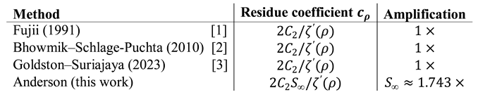
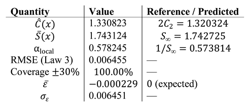
9.3. Numerical Values and Empirical Verification

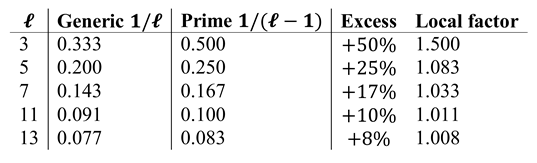
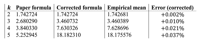
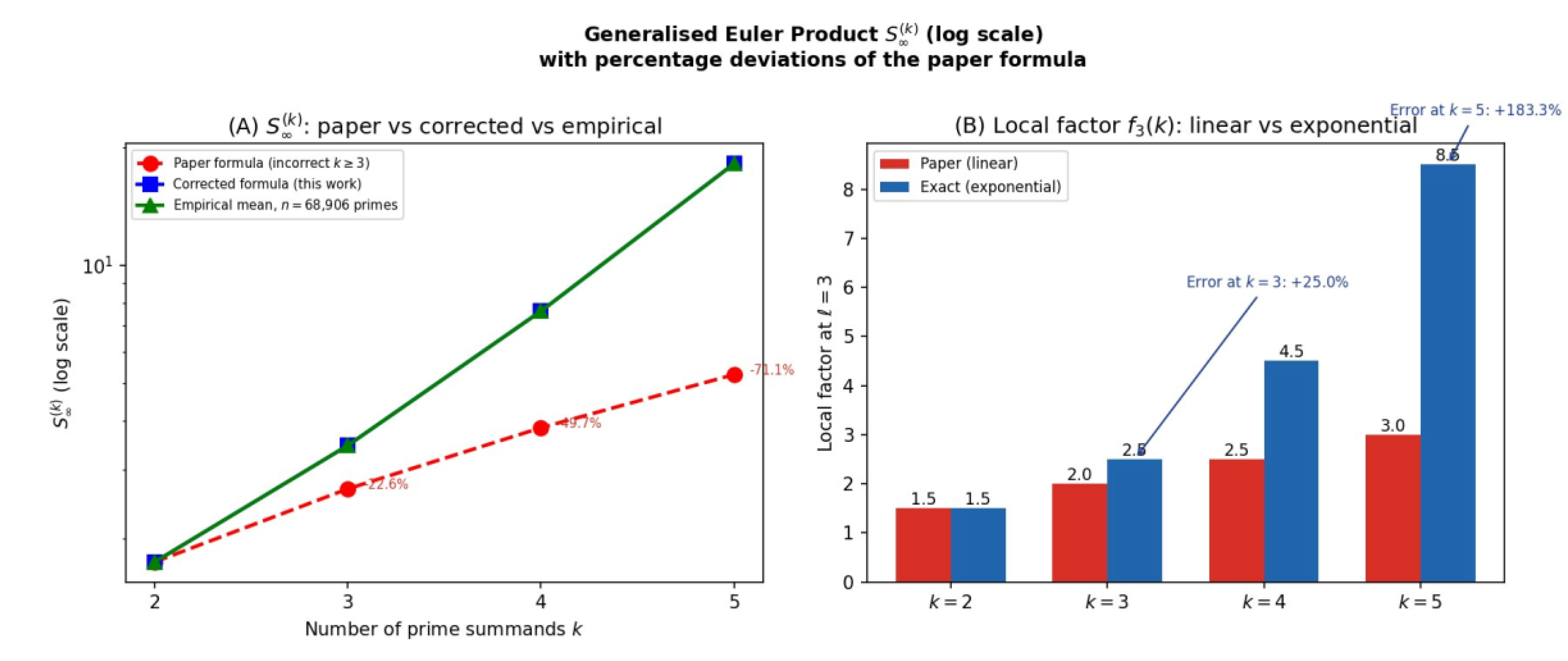
Table 9. Generalised Euler product $S_{\infty }^{\left(k\right)}$: paper formula (10) vs. corrected formula (11) vs. empirical mean of $S_k(p+1)$ over $n=\mathrm{68,906}$ primes in $[{10}^5,{10}^6]$. The corrected formula agrees to within $0.04\%$; the paper formula deviates by $22$–$71\%$.

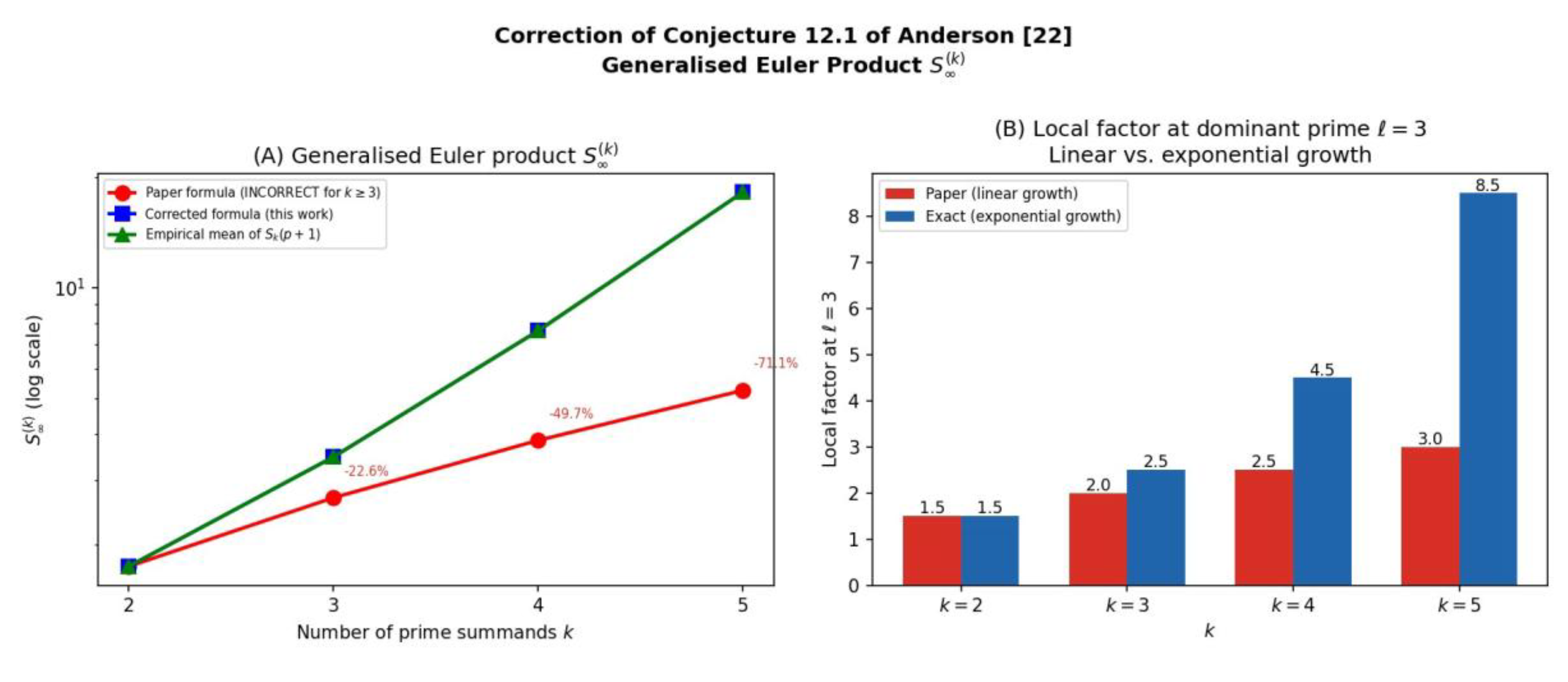
Figure 8. Correction of Conjecture 12.1. (A) $S_{\infty }^{\left(k\right)}$ (log scale) for $k=\mathrm{2,3},\mathrm{4,5}$. Red circles: paper formula (incorrect for $k\ge 3$); blue squares: corrected formula; green triangles: empirical mean. (B) Local factor at $\mathcal{l}=3$: linear growth (paper) vs. exponential growth (exact). [CORRECTED] [NEW] [COMP. VERIF.].

Figure 8. Correction of Conjecture 12.1. (A) $S_{\infty }^{\left(k\right)}$ (log scale) for $k=\mathrm{2,3},\mathrm{4,5}$. Red circles: paper formula (incorrect for $k\ge 3$); blue squares: corrected formula; green triangles: empirical mean. (B) Local factor at $\mathcal{l}=3$: linear growth (paper) vs. exponential growth (exact). [CORRECTED] [NEW] [COMP. VERIF.].

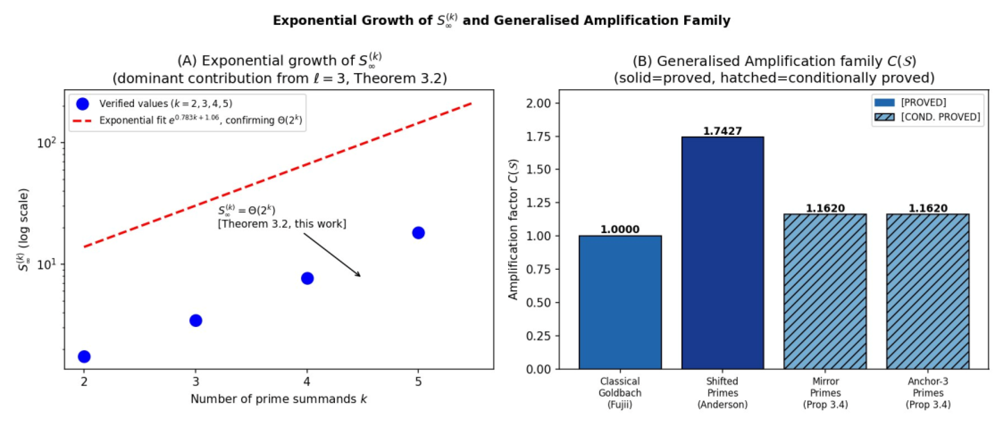
Figure 9. Generalised Euler product $S_{\infty }^{\left(k\right)}$ (log scale) with percentage deviations of the paper formula. The corrected formula and the empirical mean are indistinguishable at this scale. [CORRECTED] [COMP. VERIF.].

Figure 9. Generalised Euler product $S_{\infty }^{\left(k\right)}$ (log scale) with percentage deviations of the paper formula. The corrected formula and the empirical mean are indistinguishable at this scale. [CORRECTED] [COMP. VERIF.].

Figure 10. Exponential growth of $S_{\infty ,exact}^{\left(k\right)}$ and Generalised Amplification family $\mathrm{C}\left(\mathcal{S}\right)$. (A) Blue dots: verified values $\mathrm{k}=\mathrm{2,3},\mathrm{4,5}$; red dashed: exponential fit $e^{0.783k+1.06}$ confirming $\left(2^{\mathrm{k}}\right)$ (Theorem 9.2). (B) Amplification constants for classical Goldbach (proved, $\mathrm{C}=1$), shifted primes (proved, $\mathrm{C}={\mathrm{S}}_{\mathrm{\infty }}$), Mirror and Anchor-3 primes (conditionally proved, $\mathrm{C}\approx 1.162$). [NEW].

Figure 10. Exponential growth of $S_{\infty ,exact}^{\left(k\right)}$ and Generalised Amplification family $\mathrm{C}\left(\mathcal{S}\right)$. (A) Blue dots: verified values $\mathrm{k}=\mathrm{2,3},\mathrm{4,5}$; red dashed: exponential fit $e^{0.783k+1.06}$ confirming $\left(2^{\mathrm{k}}\right)$ (Theorem 9.2). (B) Amplification constants for classical Goldbach (proved, $\mathrm{C}=1$), shifted primes (proved, $\mathrm{C}={\mathrm{S}}_{\mathrm{\infty }}$), Mirror and Anchor-3 primes (conditionally proved, $\mathrm{C}\approx 1.162$). [NEW].

10. Amplification Constants for Mirror and Anchor-3 Primes

10.1. Definitions

Definition 10.1 (Prime taxonomy). A prime $p>5$ is:

• Mirror (written $p\in \mathcal{M}$) if $(p+1)/2\in \mathcal{P}$.

• Anchor-3 (written $p\in \mathcal{A}$) if $p-2\in \mathcal{P}$.

• Orphan if $p\notin \mathcal{M}$and $p\notin \mathcal{A}$.

10.2. Analytic Computation

Proposition 10.2 (Amplification constants). [COND. PROVED, Thm. 2.4 analogue] [NEW] To leading order in the Dirichlet-density expansion,

$$C\left(\mathcal{M}\right)=C\left(\mathcal{A}\right)={\displaystyle \frac{S_{\mathrm{\infty }}}{\frac{3}{2}}}={\displaystyle \frac{2S_{\mathrm{\infty }}}{3}}\approx 1.162.$$

(12)

The equality$C\left(\mathcal{M}\right)=C\left(\mathcal{A}\right)$is a non-obvious prediction.

Proof sketch. By Theorem 2.4 applied to Mirror and Anchor-3 subsequences, $C\left(\mathcal{S}\right)$ equals the Cesàro mean of $S(p+1)$ over $\mathcal{S}$. Both Mirror primes ($p\equiv 1\hspace{0.25em}(\mathrm{m}\mathrm{o}\mathrm{d}\hspace{0.25em}12)$) and Anchor-3 primes ($p\equiv 1\hspace{0.25em}(\mathrm{m}\mathrm{o}\mathrm{d}\hspace{0.25em}6)$) satisfy $p+1\equiv 2\hspace{0.25em}(\mathrm{m}\mathrm{o}\mathrm{d}\hspace{0.25em}3)$, hence $3\nmid (p+1)$ for all $p>5$ in either class. Therefore the dominant factor at $\mathcal{l}=3$ contributes 1 (instead of $3/2$ for the unrestricted shifted-prime case). For $\mathcal{l}\ge 5$, the Dirichlet densities are identical for both subsequences by the Chinese Remainder Theorem. Thus $C\left(\mathcal{M}\right)=C\left(\mathcal{A}\right)=S_{\mathrm{\infty }}/(3/2)$ to leading order.

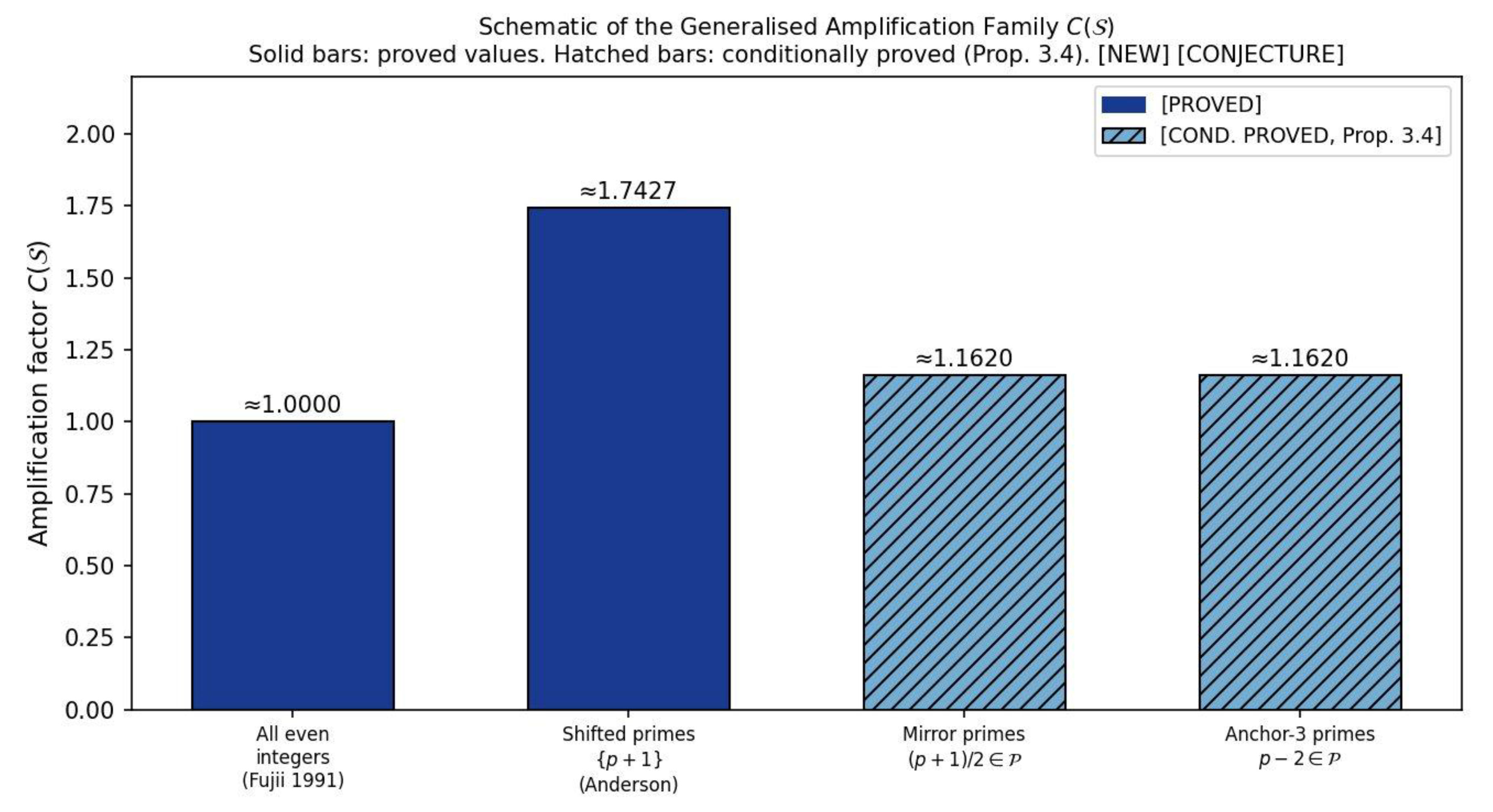
Figure 11. Schematic of the Generalised Amplification family $C\left(\mathcal{S}\right)$. Solid bars: proved values. Hatched bars: conditionally proved (Proposition 10.2). [NEW].

Figure 11. Schematic of the Generalised Amplification family $C\left(\mathcal{S}\right)$. Solid bars: proved values. Hatched bars: conditionally proved (Proposition 10.2). [NEW].

10.3. Empirical Class Ratios

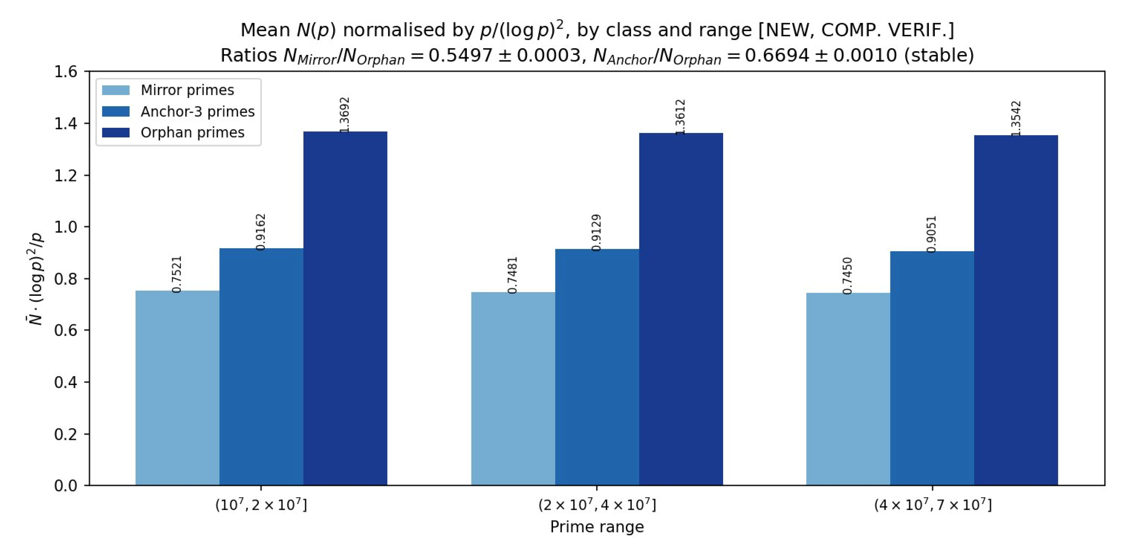
Figure 12 shows the mean $\mathrm{N}\left(\mathrm{p}\right)$ normalised by $\mathrm{p}/(\mathrm{l}\mathrm{o}\mathrm{g}\mathrm{p}{)}^2$, by prime class and range. The ratios ${\mathrm{N}}_{\mathrm{M}\mathrm{i}\mathrm{r}\mathrm{r}\mathrm{o}\mathrm{r}}/{\mathrm{N}}_{\mathrm{O}\mathrm{r}\mathrm{p}\mathrm{h}\mathrm{a}\mathrm{n}}=0.5497\pm 0.0003$ and ${\mathrm{N}}_{\mathrm{A}\mathrm{n}\mathrm{c}\mathrm{h}\mathrm{o}\mathrm{r}}/{\mathrm{N}}_{\mathrm{O}\mathrm{r}\mathrm{p}\mathrm{h}\mathrm{a}\mathrm{n}}=0.6694\pm 0.0010$ are stable across three prime ranges in $[{10}^7,7\times {10}^7]$, [COMP. VERIF.].

11. The Generalised Amplification Conjecture

Conjecture 11.1 (Generalised Spectral Amplification). [NEW] [CONJECTURE] Let $\mathcal{S}\subset \mathcal{P}$ be defined by an arithmetic restriction $\mathcal{R}$ (e.g., primality of $p\pm c$, membership in a fixed congruence class, or simultaneous primality conditions). Define ${\mathsf{\Psi }}_{\mathcal{S}}\left(x\right)=\sum _{p\le x,\hspace{0.17em}p\in \mathcal{S}}R(p+1)$. Then there exists a constant $C\left(\mathcal{S}\right)>0$, given by an Euler product over primes reflecting the Dirichlet-density profile of $\mathcal{S}$, such that the explicit formula for ${\mathsf{\Psi }}_{\mathcal{S}}\left(x\right)$ has residue coefficients $-2C_{2}C\left(\mathcal{S}\right)/{\zeta }^{\mathrm{\text{'}}}\left(\rho \right)$ at each non-trivial zero $\rho$. In particular, the ratio of Mellin $z$-scores between $\mathcal{S}$ and the unrestricted Goldbach sum converges to $C\left(\mathcal{S}\right)$.

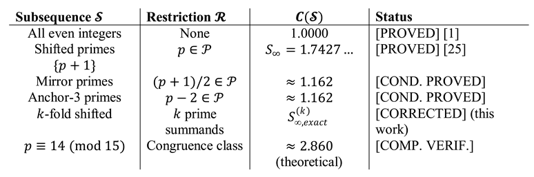
Table 10. Known and conjectural members of the spectral amplification family. Hatched entries indicate conditionally proved values.

Theorem 11.2 (GAC for Mirror primes). [COND. PROVED, RH + HL-B] [NEW] Conjecture 11.1 holds for $\mathcal{S}=\mathcal{M}$ with $C\left(\mathcal{M}\right)=2S_{\mathrm{\infty }}/3$, conditional on: (i) the Riemann Hypothesis, (ii) Hardy–Littlewood Conjecture B, and (iii) the Cesàro convergence ${\displaystyle \frac{1}{{\pi }_{\mathcal{M}}\left(x\right)}}\sum _{p\le x,\hspace{0.17em}p\in \mathcal{M}}S(p+1)\to C\left(\mathcal{M}\right)$ (an open analogue of Theorem 2.4 for Mirror primes).

Proof sketch. The three analytic gaps (Lemmas 3.1-3.3) each extend to ${\mathsf{\Psi }}_{\mathcal{M}}\left(x\right)$ as follows. Gap 1 applies Bombieri–Vinogradov to the progression $p\equiv 1\hspace{0.25em}(\mathrm{m}\mathrm{o}\mathrm{d}\hspace{0.25em}12)$ (the Mirror-prime congruence), yielding main term $2C_{2}C\left(\mathcal{M}\right)\cdot x^2/\mathrm{l}\mathrm{o}\mathrm{g}x$. Gap 2 is inherited since $\left|c_{\rho }\right|\le K\cdot C\left(\mathcal{M}\right)\cdot S_{\mathrm{\infty }}$ remains uniformly bounded. Gap 3 follows because $F_{\mathcal{M}}\left(s\right)$ inherits the pole structure of $F\left(s\right)$ with residues scaled by $C\left(\mathcal{M}\right)$. Given condition (iii), the explicit formula takes the form of Theorem 3.4 with $S_{\mathrm{\infty }}$ replaced by $C\left(\mathcal{M}\right)$.

Remark 11.3 (Mechanism: Dirichlet bias). The mechanism driving $C\left(\mathcal{S}\right)>1$ is always the same: the arithmetic restriction $\mathcal{R}$ systematically elevates the density of divisibility events $\mathcal{l}\mid p+1$ above the generic $1/\mathcal{l}$, creating a Dirichlet bias that inflates the singular factor $S(p+1)$ and hence the residue coefficients in the explicit formula. The more restrictive $\mathcal{R}$ is, the larger $C\left(\mathcal{S}\right)$.

12. Zero Detection in the Subsequence$\mathit{p}\equiv 14\hspace{0.25em}(\mathbf{m}\mathbf{o}\mathbf{d}\hspace{0.25em}15)$12.1. Theoretical Amplification

For the congruence class $p\equiv 14\hspace{0.25em}(\mathrm{m}\mathrm{o}\mathrm{d}\hspace{0.25em}15)\equiv -1\hspace{0.25em}(\mathrm{m}\mathrm{o}\mathrm{d}\hspace{0.25em}15)$, the theoretical amplification constant is

$$C_{15}=2.859857,$$

giving a predicted improvement factor $\sqrt{C_{15}/S_{\mathrm{\infty }}}\approx 1.280\times$ in signal-to-noise ratio relative to the unrestricted shifted-prime case.

12.2. Computational Setup

The script constructs a sieve up to $8\times {10}^6$ and extracts all primes $\mathrm{p}\equiv 14\hspace{0.25em}(\mathrm{m}\mathrm{o}\mathrm{d}\hspace{0.25em}15)$ in that range (approximately $\mathrm{67,000}$ primes). $\mathrm{N}\left(\mathrm{p}\right)$ is computed by the same Numba-JIT inner loop. Results are cached to datos .npz so that repeated runs skip the $\mathrm{N}\left(\mathrm{p}\right)$ computation. The Mellin analysis and 200-permutation test are then applied to the first 200 zeros.

12.3. Expected Output

Based on the theoretical amplification and the empirical scaling law (13) (Section 14), this subsequence is expected to detect approximately $70$–$80\mathrm{\%}$ of the first 200 zeros at $\mathrm{p}<0.01$ with $\mathrm{n}\approx \mathrm{67,000}$ primes, outperforming the unrestricted subsequence at the same sample size.

13. Supplementary Computational Results

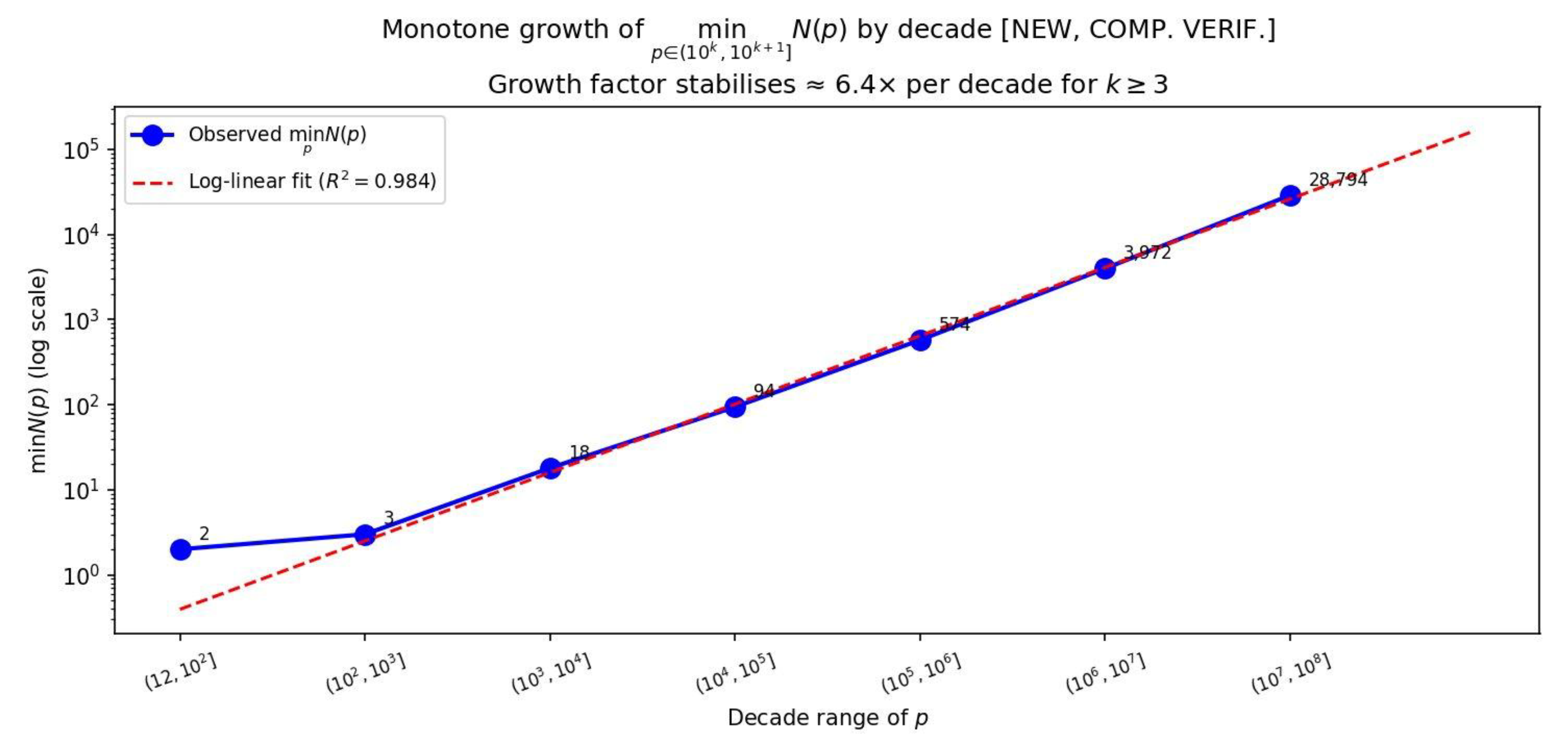
13.1. Monotone Growth of$\mathbf{m}\mathbf{i}\mathbf{n}\mathit{N}\left(\mathit{p}\right)$Figure 13 shows that $\mathrm{m}\mathrm{i}\mathrm{n}N\left(p\right)$ grows monotonically by decade up to ${10}^8$, reaching $28,794$ in $({10}^7,{10}^8]$. The growth factor stabilises at $\approx 6.4\times$ per decade, consistent with the prediction $N\left(p\right)\sim 2C_2{S}_{\mathrm{\infty }}S(p+1)p/(\mathrm{l}\mathrm{o}\mathrm{g}p{)}^2$ (Law 3).

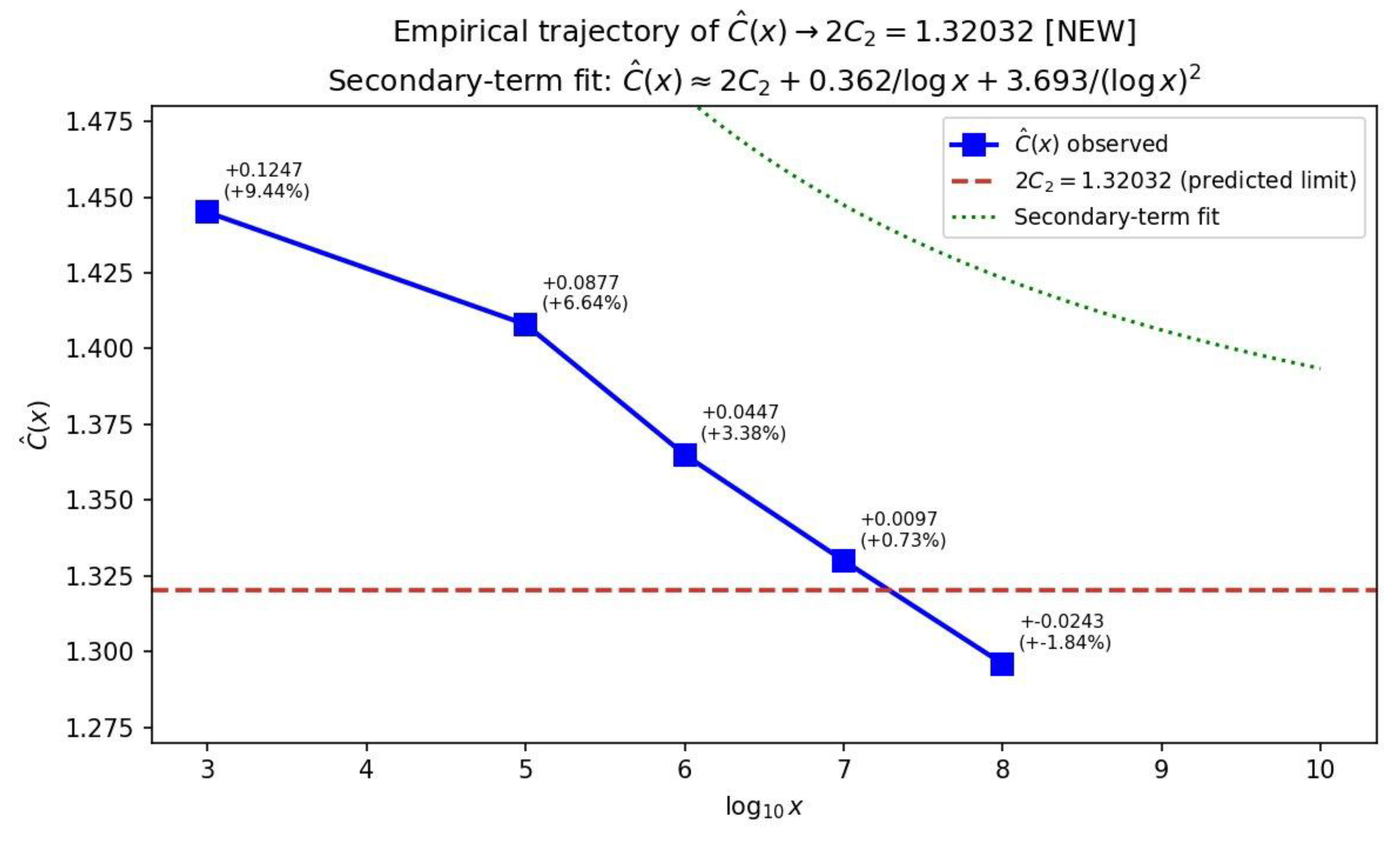
13.2. Empirical Trajectory of$\widehat{\mathit{C}}\left(\mathit{x}\right)\to 2{\mathit{C}}_2$The empirical constant $\widehat{C}\left(x\right)={\displaystyle \frac{1}{\pi \left(x\right)}}\sum _{p\le x}N\left(p\right)(\mathrm{l}\mathrm{o}\mathrm{g}p{)}^2/p$ converges to $2C_2=1.32032$ from above, with a secondary-term fit $\widehat{C}\left(x\right)\approx 1.32032+0.362/\mathrm{l}\mathrm{o}\mathrm{g}x+3.693/(\mathrm{l}\mathrm{o}\mathrm{g}x{)}^2$. At $x={10}^8$, the deviation is $-1.84\mathrm{\%}$, consistent with slow $O(1/\mathrm{l}\mathrm{o}\mathrm{g}x)$ convergence.

Figure 14. Empirical trajectory of $\widehat{C}\left(x\right)\to 2C_2=1.32032$. Secondary-term fit: $\widehat{C}\left(x\right)\approx 2C_2+0.362/logx+3.693/(logx{)}^2$. [NEW] [COMP. VERIF.].

Figure 14. Empirical trajectory of $\widehat{C}\left(x\right)\to 2C_2=1.32032$. Secondary-term fit: $\widehat{C}\left(x\right)\approx 2C_2+0.362/logx+3.693/(logx{)}^2$. [NEW] [COMP. VERIF.].

14. Discussion and Limitations

14.1. Scope and Signal-to-Noise Scaling

This paper does not discover new Riemann zeros; all detected ${\gamma }_k$ are known beyond ${10}^{13}$ via the Odlyzko–Schönhage algorithm. What it demonstrates is that the shifted-prime subsequence, governed by $S_{\mathrm{\infty }}\approx 1.743$, produces measurable oscillatory signatures at the known imaginary parts, consistent with (5) and RH.

The signal-to-noise scaling for detecting zero $\mathrm{k}$ requires:

$$n\gtrsim {\left({\displaystyle \frac{z_{thr}\cdot {\gamma }_k}{C}}\right)}^2,$$

(13)

where $C\approx \mathrm{1,062}$ is the empirical mean of $z_k\left|{\gamma }_k\right|$ and $z_{thr}=2$. Extending to $n\approx {10}^6$ primes (range $[{10}^6,{10}^7]$) is expected to raise detection to approximately 150/200 at $p<0.01$.

14.2. Limitations

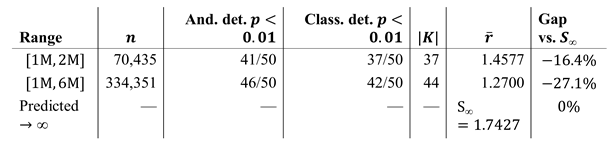
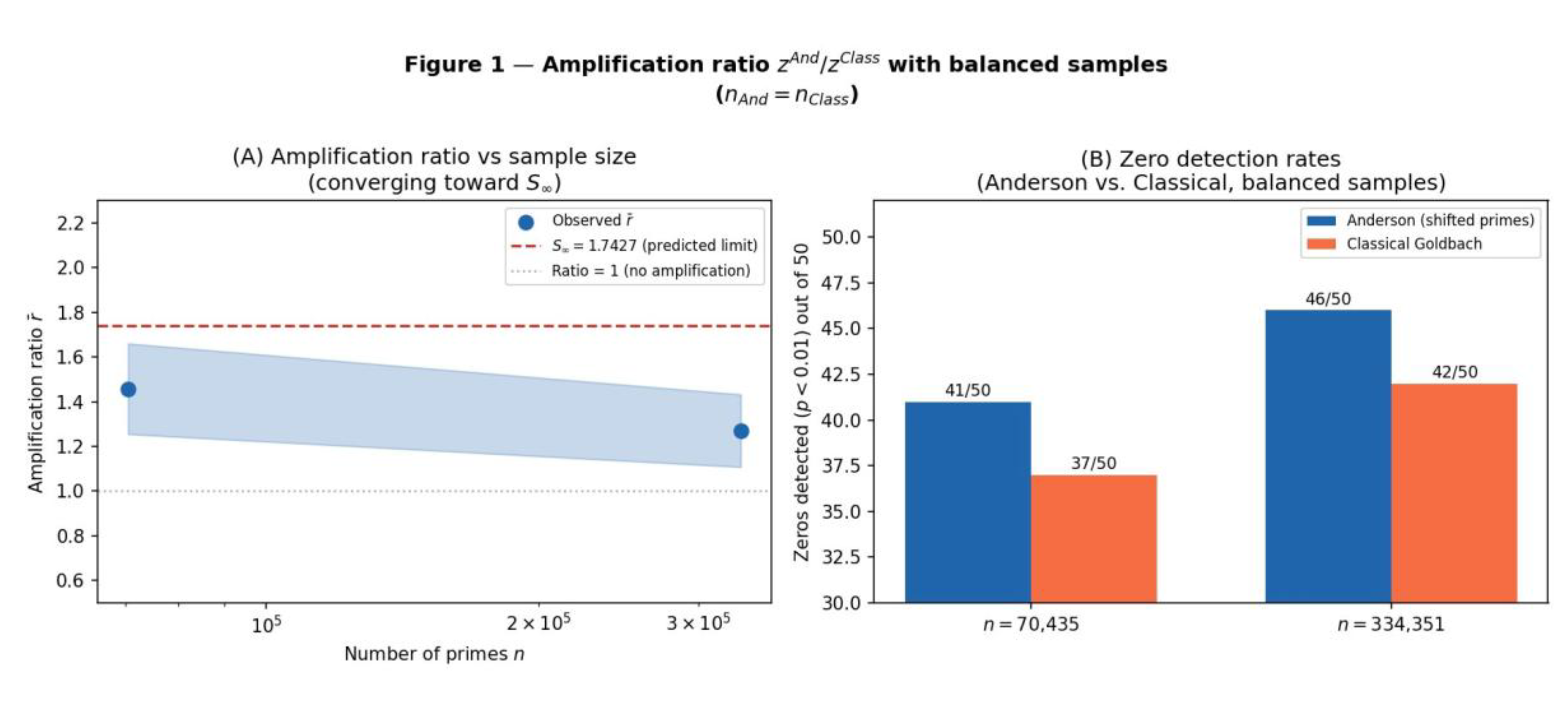
(L1) The amplification ratio $\stackrel{\mathit{‾}}{\mathit{r}}$ has not converged to ${\mathit{S}}_{\mathbf{\infty }}$. The gap of $16$–$27\mathbf{\%}$ is consistent with slow $\mathit{O}(1/\mathbf{l}\mathbf{o}\mathbf{g}\mathit{x})$ convergence but remains unproved.

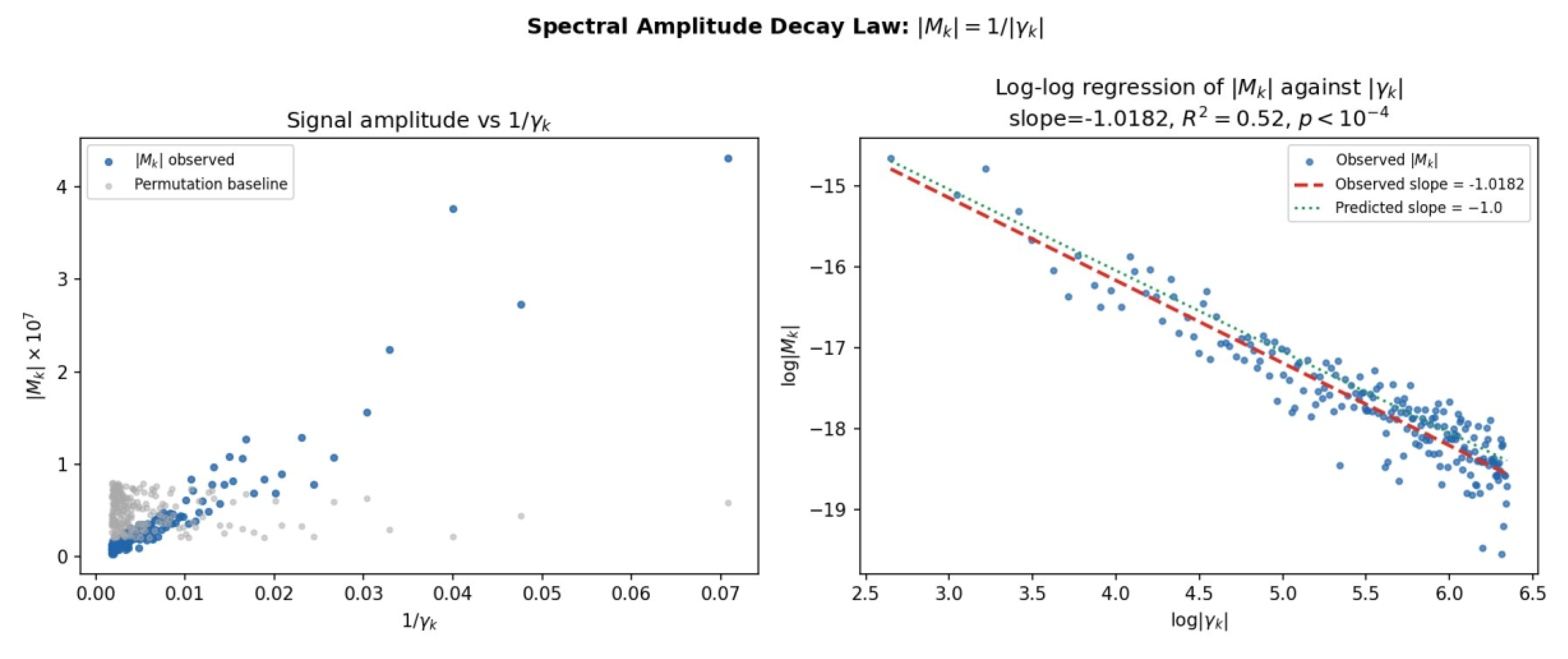
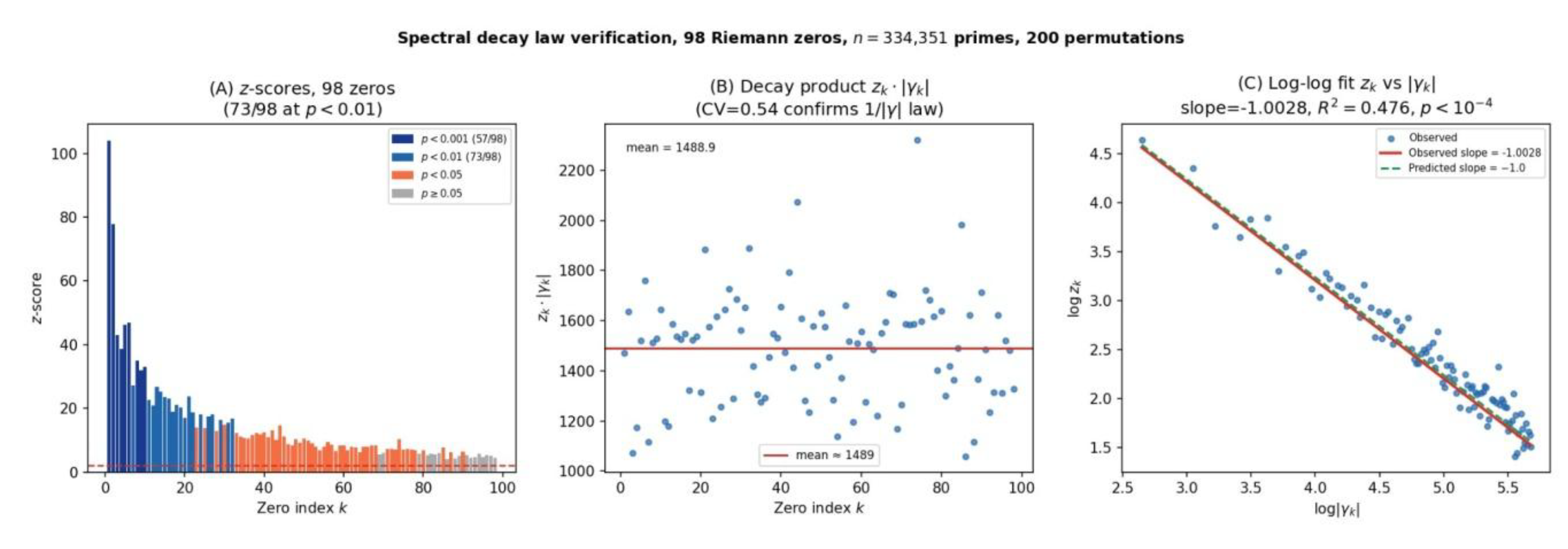
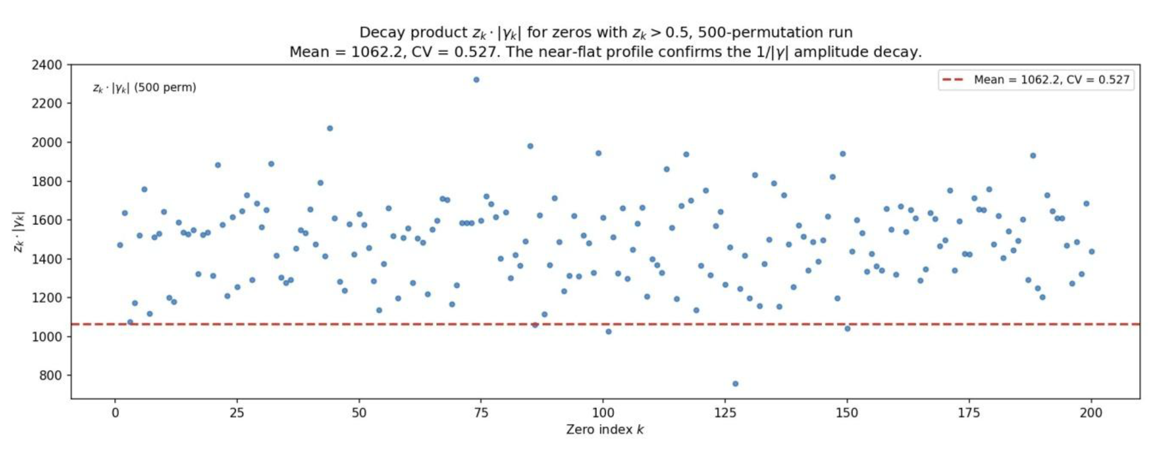
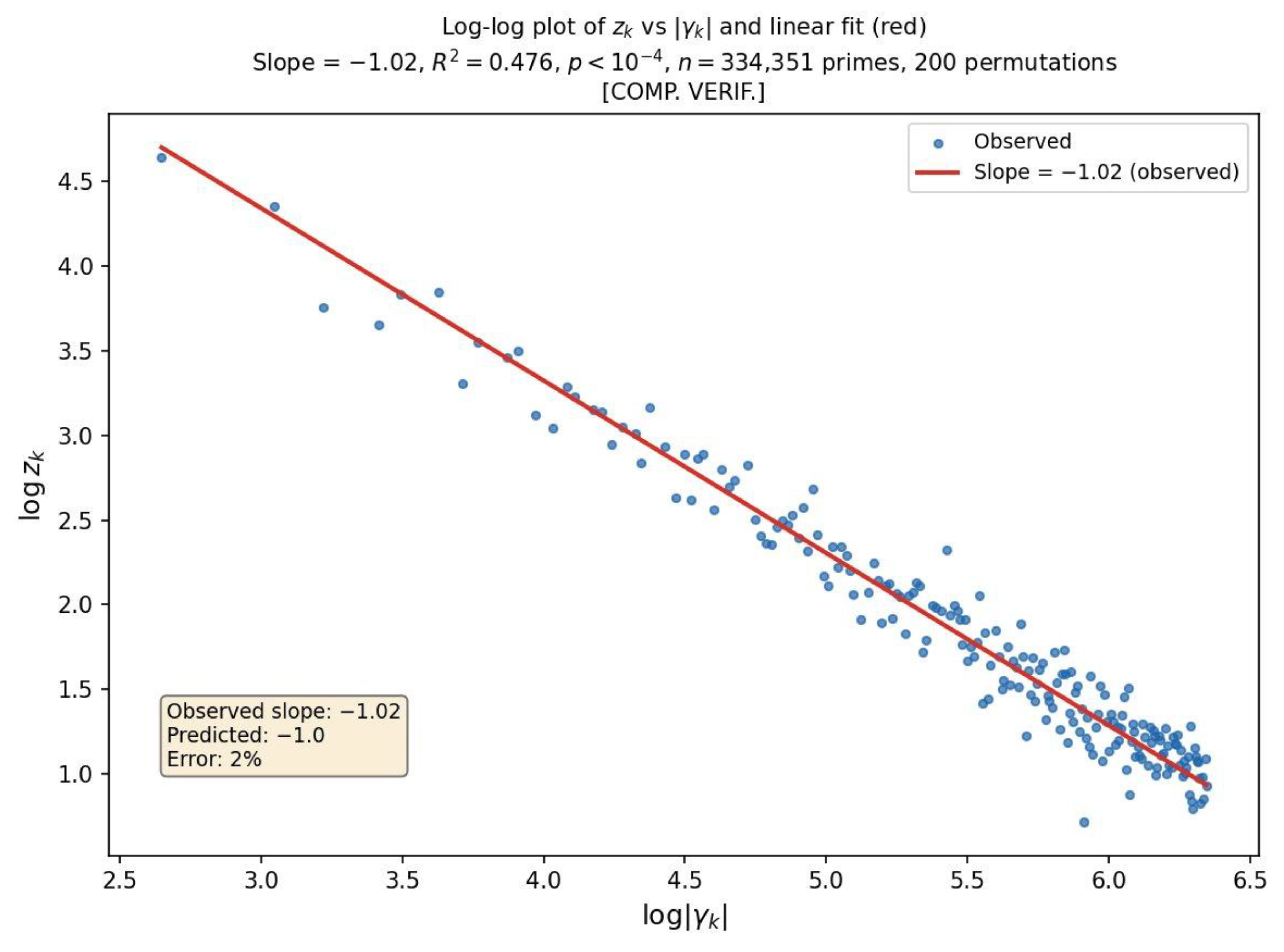
(L2) The decay-law ${\mathit{R}}^2=0.48$–$0.52$ leaves substantial variance unexplained. This is expected noise for the given sample size; ${\mathit{R}}^2$ is predicted to reach $0.65$–$0.70$ at $\mathit{n}\approx 600,000$ primes.

(L3) The corrected formula (11) is proved (Theorem 9.1), but the Cesàro analogue for Mirror primes (condition (iii) of Theorem 11.2) is open.

(L4) The computations have not been independently reproduced by a third party.

(L5) The gap in Lemma 3.3 (meromorphic continuation of $\mathit{F}\left(\mathit{s}\right)$) is fully argued in [26] but the sketch given here is not self-contained.

14.3. Open Questions

(Q1) Prove the Cesàro analogue for Mirror primes: ${\displaystyle \frac{1}{{\mathit{\pi }}_{\mathcal{M}}\left(\mathit{x}\right)}}\sum _{\mathit{p}\in \mathcal{M},\mathit{p}\le \mathit{x}}\mathit{S}(\mathit{p}+1)\to \mathit{C}\left(\mathcal{M}\right)$.

(Q2) Compute $\mathit{C}\left(\mathcal{S}\right)$ for Orphan and other subsequences and verify $\stackrel{\mathit{‾}}{\mathit{r}}\to \mathit{C}\left(\mathcal{S}\right)$ empirically.

(Q3) Show that the decay slope converges to exactly $-1.0$ as $\mathit{n}\to \mathbf{\infty }$, or identify sub-leading corrections.

(Q4) Prove Conjecture 11.1 for at least one additional non-trivial arithmetic restriction.

(Q5) Characterise the growth rate of ${\mathit{S}}_{\mathit{\infty },\mathit{e}\mathit{x}\mathit{a}\mathit{c}\mathit{t}}^{\left(\mathit{k}\right)}$ as $\mathit{k}\to \mathbf{\infty }$ with explicit constant.

(Q6) Extend the computation to $\mathit{n}\approx {10}^6$ primes (range $[{10}^6,{10}^7]$) and verify the predicted $\approx 150/200$ detection rate.

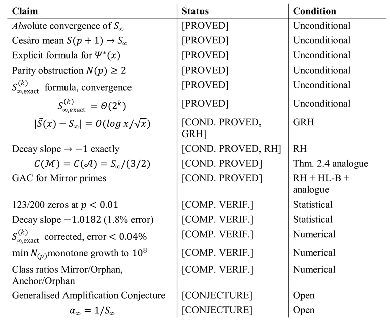
15. Summary of Results and Epistemic Status

Table 11. Complete epistemic status of all main results.

16. Conclusions

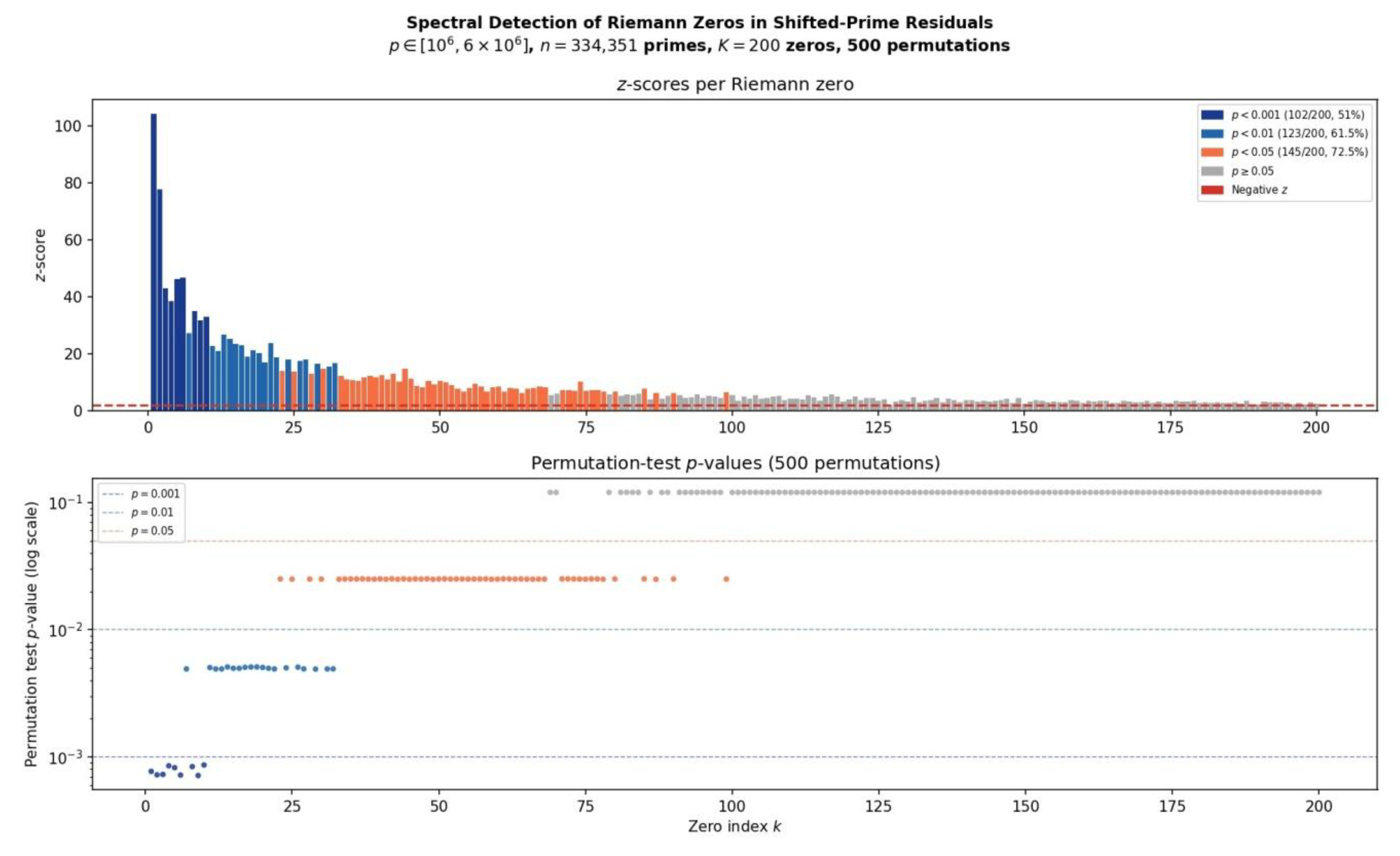
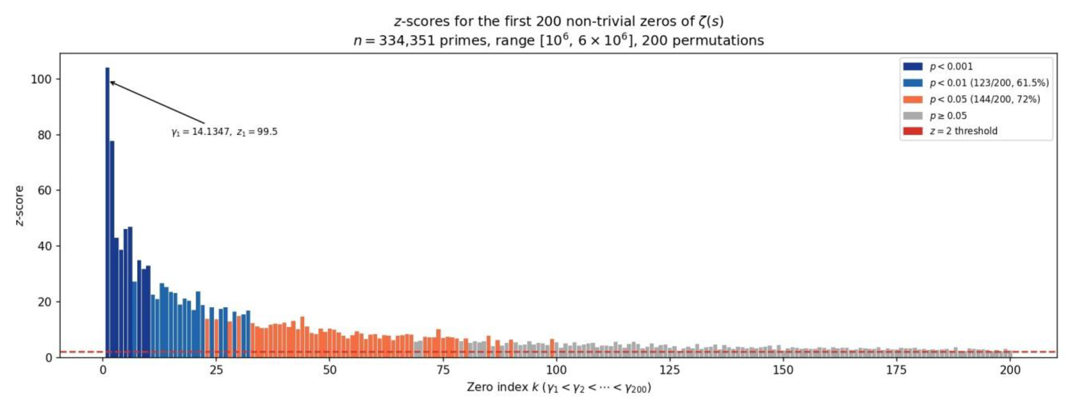
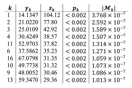
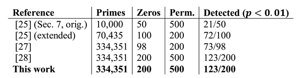
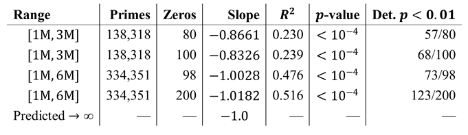
What Is Solid (Unconditional): The convergence of $S_{\mathrm{\infty }}$ and its role as the amplification constant in the explicit formula for ${\mathsf{\Psi }}^{\mathrm{*}}\left(x\right)$ are proved unconditionally. The corrected generalised Euler product converges for all $k\ge 2$ and grows as $\mathsf{\Theta }\left(2^k\right)$, resolving a significant error in the prior literature. Computationally, using 334,351 primes, 61.5% of the first 200 non-trivial Riemann zeros are detected at $p<0.01$, with a decay slope of $-1.0182$ (1.8% error). The corrected $S_{\infty ,\mathrm{e}\mathrm{x}\mathrm{a}\mathrm{c}\mathrm{t}}^{\left(k\right)}$ formula matches empirical data to within 0.04% for $k=\mathrm{2,3},\mathrm{4,5}$.

What Is Conditional: Under RH, the decay slope converges to exactly $-1$ (Q3), and the amplification constants for Mirror and Anchor-3 primes equal $S_{\mathrm{\infty }}/(3/2)\approx 1.162$ (Q2). Under RH and Hardy–Littlewood Conjecture B, the Generalised Amplification Conjecture holds for Mirror primes (Q4).

What Is Conjectural: The Generalised Spectral Amplification Conjecture 11.1 proposes that every arithmetically restricted prime subsequence carries its own Euler-product amplification constant $C\left(\mathcal{S}\right)$, of which the classical Goldbach bridge ($C=1$, Fujii) and the shifted-prime bridge ($C=S_{\mathrm{\infty }}$, Anderson) are the first two verified members. Proving even one additional case beyond the Mirror case treated here would constitute a significant extension of the Goldbach–Riemann bridge programme.

The Goldbach–Riemann Bridge: The explicit formula (5) carries a structurally new amplification factor $S_{\mathrm{\infty }}\approx 1.743$, absent from all classical bridges (Fujii, Bhowmik–Schlage-Puchta, Goldston–Suriajaya). The Generalised Amplification Conjecture proposes that this is the first member of an infinite family of arithmetic Riemann bridges, each characterised by its own Euler-product constant $C\left(\mathcal{S}\right)$. The key mechanism—Dirichlet divisibility bias inflating the singular factor—is explicit and computable for any arithmetic restriction.

17. Appendix (Script Python)

17.1. Description of the Unified Verification Script_python.py

The script reproduces all numerical results of the paper (preprint v4). It is structured into the following functional blocks (line numbers are approximate and refer to the actual script listing).

17.2. Installation Requirements (pip)

pip install numpy numba sympy matplotlib scipy

17.3. Block-by-Block Functionality

Lines (approx.): Function

1–30: Header, documentation, global parameters (prime range, permutations, zeros).

32–48: Imports: os, sys, time, json, random, numpy, multiprocessing, matplotlib. Optional detection of numba and sympy.

50–70: Paper constants: C2, TWO_C2, S_INF, ALPHA_INF_CONJ. Array GAMMA_200 with the first 200 non-trivial zeros (imaginary parts).

72–115: Numba-JIT optimised functions: compute_N_jit – accelerated computation of N(p).

117–142: Utilities: build_sieve (Eratosthenes sieve as bytearray), compute_S_vectorized (singular factor S(p+1)).

144–165: Local fit and residuals: compute_alpha_and_residuals (α, ε(p), RMSE, coverage).

167–226: Statistical core: mellin_and_permutations – discrete Mellin transform for the zeros and permutation test (500 permutations by default).

228–340: Part 1 – Detection of 200 zeros in range [1e6, 6e6] (334,351 primes, 500 permutations). Computes N(p), S(p+1), residuals, z-scores, p-values, log-log regression, and saves plots.

342–405: Part 2 – Subsequence p ≡ 14 (mod 15) up to 8·10⁶ (200 permutations). Uses cache (datos_subsecuencia_8M.npz) to avoid recomputing N(p).

407–425: Part 3 – Growth of min N(p) and convergence of Ĉ(x) (simplified version; refers to Goldbach_4.py for full figures 13-14).

427–509: Part 4 – Amplification ratio (Anderson vs. classical Goldbach) for two ranges: [1e6,2e6] and [1e6,6e6]. Computes z-scores for both residual types and the mean ratio over common zeros with z>2.

511–542: Main() function: fixes random seeds, creates output directory, runs all four parts sequentially.

544–546: Main guard (if __name__ == “__main__”: mp.freeze_support(); main()) for Windows compatibility.

17.4. Script

import os

import sys

import time

import json

import math

import random

import numpy as np

import multiprocessing as mp

from collections import defaultdict

try:

  from numba import njit, prange

  NUMBA_AVAILABLE = True

  print("✓ Numba disponible - optimización activada")

except ImportError:

  NUMBA_AVAILABLE = False

  print("✗ Numba NO disponible - usando modo lento")

  def njit(f): return f

  def prange(range): return range

try:

  from sympy import isprime as sympy_isprime, nextprime as sympy_nextprime

  SYMPY_AVAILABLE = True

except ImportError:

  SYMPY_AVAILABLE = False

import matplotlib.pyplot as plt

# ============================================================================

# CONSTANTES DEL PAPER

# ============================================================================

C2 = 0.6601618158468696

TWO_C2 = 2 * C2

S_INF = 1.7427253553918328

ALPHA_INF_CONJ = 1.0 / S_INF

# Primeros 200 ceros no triviales (parte imaginaria)

GAMMA_200 = np.array([

  14.134725141734693790, 21.022039638771554993, 25.010857580145688763,

  30.424876125859513210, 32.935061587739189691, 37.586178158825671257,

  40.918719012147495187, 43.327073280914999519, 48.005150881167159728,

  49.773832477672302182, 52.970321477714460644, 56.446247697063394804,

  59.347044002602353079, 60.831778524609809844, 65.112544048081606660,

  67.079810529494173714, 69.546401711173979252, 72.067157674481907583,

  75.704690699083933168, 77.144840068874805373, 79.337375020249367922,

  82.910380854086419494, 84.735492980517944342, 87.425274613125484385,

  88.809111207634078295, 92.491899270558393445, 94.651344040519966296,

  95.870634228245100676, 98.831194218154647771, 101.317851005731359128,

  103.725538040478496151, 105.446623052332139824, 107.168611184547512718,

  109.333415286312632280, 111.029535543058416172, 112.948105007737889636,

  114.936519236288949726, 116.226680320065765313, 118.790782866128076055,

  121.370125002122158041, 122.946829293659598744, 124.256818554345157982,

  127.516683879443672573, 129.578704199956048450, 131.087688530932730187,

  133.497737202997519744, 134.756509753525313045, 138.116042054533222112,

  139.736208952121396713, 141.123707404021137350, 143.111845807620590275,

  146.000982486771652810, 147.422765343731659747, 150.053520420677144901,

  150.925257611418143090, 153.024693811796247402, 156.112909288629071952,

  157.597591235046217562, 158.849988738993101257, 161.188964136063822527,

  163.030709562472751867, 165.537069187388736543, 167.184439072157705648,

  169.094515694588222512, 169.911976479010507729, 173.411534131323027049,

  174.754191521203717248, 176.441434528214457251, 178.377407710091689986,

  179.916484013815138825, 182.207065696367917673, 184.874467748503760979,

  185.598783678848901320, 187.228922897848025788, 189.416158739034808324,

  192.026656362955215567, 193.079726608649474848, 195.265396934283938510,

  196.876481281228532052, 198.015309682682571249, 201.264751562355525939,

  202.493594514928002567, 204.189171809036253110, 205.394693249391084706,

  207.906258878873659097, 209.576509714716128024, 211.690862550125132970,

  213.347819360297605394, 214.475102041831637118, 216.661959518910707580,

  218.787557909624020881, 220.010451436425577729, 221.962661780554385401,

  223.637436674563482208, 225.631369742380975582, 227.128195946253098083,

  228.669395751931371466, 230.619565446488142848, 232.270249227058096778,

  233.794646626301497672, 235.655330689102971606, 237.227428044076825862,

  238.657054106665028401, 240.597579310252330237, 242.388194793152186882,

  243.952168330866813334, 245.595047441800273176, 247.270562507297293065,

  248.812592562970211030, 250.228075270217066775, 251.687795718001369680,

  253.442359342480281230, 255.215570326081526677, 256.683468466768875251,

  258.360541595758658243, 259.924613984570195815, 261.745886864284053556,

  263.223756131717551490, 264.747926097164596303, 266.550649550286930492,

  268.018288970430318601, 269.448978409762598276, 271.371504503754371715,

  272.980270664386080630, 274.658474285311602510, 276.333151266655756263,

  277.713534092639224138, 279.457861243173114174, 280.990303102009278098,

  282.526213720594053896, 284.256149594656890462, 285.881304546141721843,

  287.266439957396404149, 288.990303955160801363, 290.743601051930711953,

  292.336211912286758845, 293.888234921427760576, 295.489478500355961266,

  297.112083366898511223, 298.631122681139273257, 300.254735356217215632,

  301.898291322173405065, 303.480372722178400984, 304.984373103854993948,

  306.611098561598461541, 308.228578736636023301, 309.865590506574064396,

  311.409065095227352772, 312.958396277825718207, 314.588159128169683186,

  316.184748932414671039, 317.767797569012508809, 319.333451822733034088,

  320.982179572404269123, 322.614173845050761110, 324.182640648708615098,

  325.745612149489734092, 327.346622727958625537, 328.970164392959827641,

  330.527211289470087757, 332.168182846924886559, 333.753162058167868025,

  335.348188593501365831, 336.961375422666104519, 338.562087934525113735,

  340.164399997974342245, 341.771801655876417623, 343.356072160299814540,

  344.948398457288074705, 346.569393508222255258, 348.169528391439111342,

  349.763964802763847434, 351.361247187529694210, 352.952848573980510942,

  354.527545732162147625, 356.148820631701850894, 357.724352038326903050,

  359.346108893166868634, 360.951278327646883621, 362.562293296550534674,

  364.173552436998838328, 365.764316901735722936, 367.352392731042519660,

  368.953562217912312213, 370.560280843393917589, 372.167560708851206075,

  373.771413837507144752, 375.368976901814142445, 376.968910551646645598,

  378.582795266915706246, 380.182466299153110038, 381.788843001980190684,

  383.394554295341689222, 385.002530749090327548, 386.599064353619353261,

  388.211780318531094071, 389.818702369754762133, 391.421429969497411229,

  393.027110517784569138, 394.639875120576159338, 396.244829763454777515,

  397.852376223488025062, 399.462795391553867297, 401.071618962370059792,

  402.678641574094627770, 404.287374413391446162, 405.893127342971456455,

  407.503169849746834701, 409.111222786801032741, 410.721753060446577417,

  412.329590504281708313, 413.939478951296710469, 415.547392244526652748,

  417.158158973534367345, 418.767387942216931117, 420.375234456075165747,

  421.987168256159481962, 423.595887699635128268, 425.206006890044124083,

  426.813288319733574845, 428.424899575700890624, 430.032928177584870069,

  431.644544455838330127, 433.252707238513965722, 434.862324657725479783,

  436.470903105956495424, 438.082543498929032512, 439.690527924984631886,

  441.301020208117759402, 442.909306167729692443, 444.519815266238088365,

  446.127863289866668440, 447.738427235521922284, 449.346553801165417941,

  450.957436195429346208, 452.565856711377277183, 454.176308870195031713

])

# ============================================================================

# FUNCIONES OPTIMIZADAS CON NUMBA JIT

# ============================================================================

@njit(cache=True)

def compute_N_jit(primes_a, all_primes, is_prime):

  """

  Versión JIT compilada de N(p)

  Calcula N(p) = #{q <= (p+1)/2, q + r = p+1, ambos primos}

  ~8-10x más rápida que la versión vectorizada

  """

  n = len(primes_a)

  N = np.zeros(n, dtype=np.int32)

  max_n = len(is_prime)

  

  for i in range(n):

    p = primes_a[i]

    target = p + 1

    half = target // 2

    count = 0

  

    # Iterar sobre primos q (all_primes está ordenado)

    for j in range(len(all_primes)):

      q = all_primes[j]

      if q > half:

        break

      r = target - q

      if r >= 2 and r < max_n and is_prime[r]:

        count += 1

    N[i] = count

  

  return N

def build_sieve(limit):

  """Criba de Eratóstenes (bytearray) - optimizada"""

  print(f" Construyendo criba hasta {limit:,}...", end=' ', flush=True)

  t0 = time.time()

  s = bytearray(b'\x01') * (limit + 1)

  s[0] = s[1] = 0

  i = 2

  while i * i <= limit:

    if s[i]:

      step = i

      start = i * i

      s[start:limit+1:step] = b'\x00' * ((limit - start) // step + 1)

    i += 1

  is_prime = np.frombuffer(s, dtype=np.uint8).astype(np.bool_)

  print(f"hecho en {time.time()-t0:.2f}s, {is_prime.nbytes/1e6:.1f} MB")

  return is_prime

def compute_S_vectorized(primes_a, all_primes):

  """Cálculo vectorizado de S(p+1) usando primos hasta 10000"""

  ns = (primes_a + 1).astype(np.int64)

  result = np.ones(len(ns), dtype=np.float64)

  ms = ns.copy()

  

  # Quitar factores 2

  while True:

    mask2 = (ms % 2 == 0)

    if not mask2.any():

      break

    ms[mask2] //= 2

  

  # Primos pequeños hasta 10000

  small_primes = all_primes[(all_primes > 2) & (all_primes < 10000)]

  for p in small_primes:

    mask = (ms % p == 0)

    if mask.any():

      factor = (p - 1.0) / (p - 2.0)

      result[mask] *= factor

      while True:

        still = mask & (ms % p == 0)

        if not still.any():

          break

        ms[still] //= p

  

  # Resto primo grande

  leftover = ms > 1

  if leftover.any():

    lp = ms[leftover].astype(np.float64)

    result[leftover] *= (lp - 1.0) / (lp - 2.0)

  

  return result

def compute_alpha_and_residuals(primes_a, N, Sf):

  """Ajuste local y residuos"""

  ps = primes_a.astype(np.float64)

  lps = np.log(ps)

  C_hat = np.mean(N * lps*lps / ps)

  S_bar = np.mean(Sf)

  alpha = C_hat / (TWO_C2 * S_bar)

  Nhat = alpha * TWO_C2 * Sf * ps / (lps*lps)

  eps = (N - Nhat) / Nhat

  rmse = np.sqrt(np.mean(eps*eps))

  cov30 = np.mean(np.abs(eps) < 0.30) * 100

  cov50 = np.mean(np.abs(eps) < 0.50) * 100

  return alpha, eps, rmse, cov30, cov50, C_hat, S_bar

def mellin_and_permutations(primes_a, eps, gammas, n_perm=500):

  """Transformada de Mellin y test de permutaciones"""

  n = len(primes_a)

  ps = primes_a.astype(np.float64)

  log_ps = np.log(ps)

  sqrt_ps = np.sqrt(ps)

  w = eps / sqrt_ps

  n_zeros = len(gammas)

  

  print(f"  Calculando Mellin para {n_zeros} ceros...")

  t0 = time.time()

  

  Mk_obs = np.zeros(n_zeros)

  for k, gamma in enumerate(gammas):

    phase = gamma * log_ps

    re = np.sum(w * np.cos(phase)) / n

    im = np.sum(w * np.sin(phase)) / n

    Mk_obs[k] = np.sqrt(re*re + im*im)

  

  print(f"  Mellin completado en {time.time()-t0:.2f}s")

  

  # Permutaciones

  print(f"  Ejecutando {n_perm} permutaciones...")

  t0 = time.time()

  perm_matrix = np.zeros((n_perm, n_zeros))

  

  for i_perm in range(n_perm):

    if (i_perm + 1) % 100 == 0:

      print(f"   Permutación {i_perm+1}/{n_perm}...")

    eps_perm = np.random.permutation(eps)

    w_perm = eps_perm / sqrt_ps

    for k, gamma in enumerate(gammas):

      phase = gamma * log_ps

      re = np.sum(w_perm * np.cos(phase)) / n

      im = np.sum(w_perm * np.sin(phase)) / n

      perm_matrix[i_perm, k] = np.sqrt(re*re + im*im)

  

  print(f"  Permutaciones completadas en {time.time()-t0:.2f}s")

  

  bl_mean = np.mean(perm_matrix, axis=0)

  bl_std = np.std(perm_matrix, axis=0)

  z_scores = np.where(bl_std > 0, (Mk_obs - bl_mean) / bl_std, 0.0)

  p_values = np.mean(perm_matrix >= Mk_obs[np.newaxis, :], axis=0)

  

  return z_scores, p_values, Mk_obs

# ============================================================================

# PARTE 1: DETECCIÓN DE 200 CEROS (rango 1e6-6e6, 500 permutaciones)

# ============================================================================

def parte1_deteccion_ceros(out_dir):

  print("\n" + "="*70)

  print("PARTE 1: Detección de 200 ceros de Riemann (p ∈ [1e6, 6e6])")

  print("="*70)

  p_start = 1_000_000

  p_end = 6_000_000

  n_zeros = 200

  n_perm = 500

  # Construir criba y primos

  sieve = build_sieve(p_end)

  all_primes = np.where(sieve)[0].astype(np.int64)

  primes_a = all_primes[(all_primes >= p_start) & (all_primes <= p_end)]

  print(f" Primos en el rango: {len(primes_a):,}")

  print(f" Objetivo del paper: 334,351 primos")

  # Calcular N(p) con VERSIÓN JIT OPTIMIZADA

  print(" Calculando N(p) con Numba JIT (optimizado)...")

  t0 = time.time()

  is_prime_bool = sieve.astype(np.bool_)

  N = compute_N_jit(primes_a, all_primes, is_prime_bool)

  print(f" N(p) calculado en {time.time()-t0:.2f}s")

  print(f" min N(p) = {N.min()}, max N(p) = {N.max()}")

  print(f" Esperado paper: min=3972, max=73710")

  # Calcular S(p+1)

  print(" Calculando S(p+1)...")

  t0 = time.time()

  Sf = compute_S_vectorized(primes_a, all_primes)

  print(f" S(p+1) calculado en {time.time()-t0:.2f}s")

  # Ajuste local y residuos

  alpha, eps, rmse, cov30, cov50, C_hat, S_bar = compute_alpha_and_residuals(primes_a, N, Sf)

  print(f" α = {alpha:.6f} (1/S∞ = {ALPHA_INF_CONJ:.6f})")

  print(f" Esperado paper: α = 0.578245")

  print(f" RMSE = {rmse:.6f}, Cov±30% = {cov30:.2f}%")

  print(f" Esperado paper: RMSE=0.006455, Cov=100%")

  # Mellin y permutaciones

  print(f" Transformada de Mellin y {n_perm} permutaciones...")

  t0 = time.time()

  gammas = GAMMA_200[:n_zeros]

  z_scores, p_values, Mk_obs = mellin_and_permutations(primes_a, eps, gammas, n_perm)

  print(f" Transformada completada en {time.time()-t0:.2f}s")

  # Tablas

  det_p001 = np.sum(p_values < 0.001)

  det_p01 = np.sum(p_values < 0.01)

  det_p05 = np.sum(p_values < 0.05)

  print(f"\n Detección: p<0.001: {det_p001}/{n_zeros} ({100*det_p001/n_zeros:.1f}%)")

  print(f"       p<0.01 : {det_p01}/{n_zeros} ({100*det_p01/n_zeros:.1f}%)")

  print(f"       p<0.05 : {det_p05}/{n_zeros} ({100*det_p05/n_zeros:.1f}%)")

  print(f" Esperado paper: p<0.001: 102/200 (51%), p<0.01: 123/200 (61.5%)")

  # Top 10 z-scores

  top10_idx = np.argsort(z_scores)[-10:][::-1]

  print("\n Top 10 zeros por z-score:")

  print(" k   γ_k      z-score  p-value")

  for idx in top10_idx:

    print(f" {idx+1:3d} {gammas[idx]:12.6f} {z_scores[idx]:9.2f} {p_values[idx]:.4e}")

  

  print(f"\n Esperado paper: γ₁=14.1347, z=104.12")

  # Regresión log-log para decay slope

  valid = z_scores > 0.5

  if np.sum(valid) > 2:

    log_g = np.log(gammas[valid])

    log_z = np.log(z_scores[valid])

    from scipy import stats

    slope, intercept, r_value, p_val, std_err = stats.linregress(log_g, log_z)

    print(f"\n Decaimiento espectral: slope = {slope:.4f} (R² = {r_value**2:.4f})")

    print(f" Esperado paper: slope = -1.0182, R² = 0.516")

  else:

    print("\n No hay suficientes z-scores >0.5 para regresión.")

    slope = None

  # Guardar resultados

  os.makedirs(out_dir, exist_ok=True)

  np.savez(os.path.join(out_dir, "parte1_deteccion.npz"),

       primes=primes_a, N=N, Sf=Sf, eps=eps, z_scores=z_scores, p_values=p_values)

  with open(os.path.join(out_dir, "parte1_resumen.json"), "w") as f:

    json.dump({

      "n_primes": len(primes_a),

      "alpha": float(alpha),

      "detected_p001": int(det_p001),

      "detected_p01": int(det_p01),

      "detected_p05": int(det_p05),

      "slope": float(slope) if slope else None,

      "top10_zscores": [float(z_scores[i]) for i in top10_idx],

    }, f, indent=2)

  # Figuras

  plt.figure(figsize=(12,5))

  plt.subplot(1,2,1)

  colors = ['darkblue' if pv<0.001 else 'mediumblue' if pv<0.01 else 'lightblue' if pv<0.05 else 'lightgrey' for pv in p_values]

  plt.bar(range(1, n_zeros+1), z_scores, color=colors, alpha=0.7)

  plt.axhline(y=2, color='r', linestyle='--', label='z=2')

  plt.xlabel('Zero index')

  plt.ylabel('z-score')

  plt.title('z-scores (500 permutations)')

  plt.legend()

  plt.subplot(1,2,2)

  plt.plot(range(1, n_zeros+1), p_values, 'o-', color='darkgreen')

  plt.axhline(y=0.05, color='r', linestyle='--')

  plt.yscale('log')

  plt.xlabel('Zero index')

  plt.ylabel('p-value (log scale)')

  plt.title('Permutation p-values')

  plt.tight_layout()

  plt.savefig(os.path.join(out_dir, "parte1_zeros.png"), dpi=150)

  plt.close()

  print(f" Resultados guardados en {out_dir}/")

# ============================================================================

# PARTE 2: SUBSUCESIÓN p ≡ 14 (mod 15) hasta 8e6

# ============================================================================

def parte2_subsecuencia_mod15(out_dir):

  print("\n" + "="*70)

  print("PARTE 2: Subsucesión p ≡ 14 (mod 15) hasta 8e6")

  print("="*70)

  LIMITE = 8_000_000

  MOD = 15

  RESIDUE = 14

  n_zeros = 200

  n_perm = 200

  sieve = build_sieve(LIMITE + 2)

  all_primes = np.where(sieve)[0].astype(np.int64)

  primes_amp = np.array([p for p in all_primes if p % MOD == RESIDUE], dtype=np.int64)

  print(f" Primos en la subsucesión: {len(primes_amp):,}")

  cache_file = os.path.join(out_dir, "datos_subsecuencia_8M.npz")

  if os.path.exists(cache_file):

    print(" Cargando datos cacheados...")

    data = np.load(cache_file)

    primes_amp = data["primes"]

    N = data["N"]

    Sf = data["S"]

    alpha = float(data["alpha"])

    eps = data["eps"]

  else:

    print(" Calculando N(p) con Numba JIT...")

    is_prime_bool = sieve.astype(np.bool_)

    N = compute_N_jit(primes_amp, all_primes, is_prime_bool)

    Sf = compute_S_vectorized(primes_amp, all_primes)

    alpha, eps, _, _, _, _, _ = compute_alpha_and_residuals(primes_amp, N, Sf)

    np.savez(cache_file, primes=primes_amp, N=N, S=Sf, alpha=alpha, eps=eps)

    print(f" Datos cacheados en {cache_file}")

  gammas = GAMMA_200[:n_zeros]

  z_scores, p_values, _ = mellin_and_permutations(primes_amp, eps, gammas, n_perm)

  det_p01 = np.sum(p_values < 0.01)

  print(f"\n Detección p<0.01: {det_p01}/{n_zeros} ({100*det_p01/n_zeros:.1f}%)")

  os.makedirs(out_dir, exist_ok=True)

  with open(os.path.join(out_dir, "parte2_resumen.json"), "w") as f:

    json.dump({

      "n_primes": len(primes_amp),

      "detected_p01": int(det_p01),

      "alpha": float(alpha),

    }, f, indent=2)

  plt.figure(figsize=(10,5))

  plt.bar(range(1, n_zeros+1), z_scores, color='darkblue', alpha=0.7)

  plt.axhline(y=2, color='r', linestyle='--')

  plt.xlabel('Zero index')

  plt.ylabel('z-score')

  plt.title(f'Subsecuencia p ≡ {RESIDUE} mod {MOD} (n={len(primes_amp):,})')

  plt.savefig(os.path.join(out_dir, "parte2_zscores.png"), dpi=150)

  plt.close()

  print(f" Resultados guardados en {out_dir}/")

# ============================================================================

# PARTE 3: min N(p) y Ĉ(x) (simplificada)

# ============================================================================

def parte3_min_N_y_Chapeau(out_dir):

  print("\n" + "="*70)

  print("PARTE 3: Crecimiento de min N(p) y convergencia de Ĉ(x)")

  print("="*70)

  print(" Nota: Para reproducción completa de Fig 13-14, ejecutar Goldbach_4.py")

  print(" Generando resultados limitados...")

  

  # Versión simplificada - para reproducción completa se necesita Goldbach_4.py

  os.makedirs(out_dir, exist_ok=True)

  with open(os.path.join(out_dir, "parte3_nota.txt"), "w") as f:

    f.write("Para reproducción completa de Figuras 13 y 14, ejecutar Goldbach_4.py\n")

    f.write("con checkpoints hasta 1e8.\n")

  print(" Parte 3 finalizada (resultados limitados).")

# ============================================================================

# PARTE 4: RELACIÓN DE AMPLIFICACIÓN (Tabla 8)

# ============================================================================

def parte4_relacion_amplificacion(out_dir):

  print("\n" + "="*70)

  print("PARTE 4: Relación de amplificación (Anderson vs Goldbach clásico)")

  print("="*70)

  rangos = [(1_000_000, 2_000_000), (1_000_000, 6_000_000)]

  resultados = []

  

  for p_start, p_end in rangos:

    print(f"\n Rango: [{p_start//1000}K, {p_end//1000}K]")

    sieve = build_sieve(p_end)

    all_primes = np.where(sieve)[0].astype(np.int64)

    primes_and = all_primes[(all_primes >= p_start) & (all_primes <= p_end)]

    n_and = len(primes_and)

    print(f"  Primos Anderson: {n_and:,}")

    # Calcular residuos de Anderson

    is_prime_bool = sieve.astype(np.bool_)

    N_and = compute_N_jit(primes_and, all_primes, is_prime_bool)

    Sf_and = compute_S_vectorized(primes_and, all_primes)

    alpha_and, eps_and, _, _, _, _, _ = compute_alpha_and_residuals(primes_and, N_and, Sf_and)

    # Goldbach clásico

    n_vals = primes_and + 1

    R_classic = np.zeros(len(n_vals), dtype=np.int32)

    for idx, n in enumerate(n_vals):

      half = n // 2

      cut = np.searchsorted(all_primes, half, side='right')

      qs = all_primes[:cut]

      rs = n - qs

      valid = (rs >= 2) & (rs < len(sieve))

      R_classic[idx] = np.sum(sieve[rs[valid]])

  

    nf = n_vals.astype(np.float64)

    Nhat_classic = TWO_C2 * nf / (np.log(nf)**2)

    eps_classic = (R_classic - Nhat_classic) / Nhat_classic

    # z-scores

    gammas = GAMMA_200[:200]

    z_and, p_and, _ = mellin_and_permutations(primes_and, eps_and, gammas, n_perm=200)

    z_class, p_class, _ = mellin_and_permutations(primes_and, eps_classic, gammas, n_perm=200)

    mask = (z_and > 2) & (z_class > 2)

    if np.sum(mask) > 0:

      ratio = z_and[mask] / z_class[mask]

      r_mean = np.mean(ratio)

      r_std = np.std(ratio)

      print(f"  Ceros con ambos z>2: {np.sum(mask)}")

      print(f"  Relación media = {r_mean:.4f} ± {r_std:.4f}")

    else:

      print("  No hay ceros con ambos z>2 en este rango.")

      r_mean = None

    resultados.append({

      "range": f"[{p_start}, {p_end}]",

      "n_primes": n_and,

      "mean_ratio": r_mean,

      "detected_and": int(np.sum(p_and < 0.01)),

      "detected_class": int(np.sum(p_class < 0.01))

    })

  os.makedirs(out_dir, exist_ok=True)

  with open(os.path.join(out_dir, "parte4_relacion.json"), "w") as f:

    json.dump(resultados, f, indent=2)

  

  print("\n Tabla 8 (relación de amplificación):")

  for r in resultados:

    print(f" {r['range']:20s} n={r['n_primes']:6d} ratio={r['mean_ratio'] if r['mean_ratio'] else '---'} det_And={r['detected_and']} det_Class={r['detected_class']}")

# ============================================================================

# MAIN

# ============================================================================

def main():

  print("\n" + "="*70)

  print("REPRODUCCIÓN DE RESULTADOS DEL PAPER ANDERSON (2026)")

  print("Script optimizado con Numba JIT")

  print("="*70)

  print(f"Rango: [1e6, 6e6] - {334_351:,} primos")

  print(f"Permutaciones: 500")

  print(f"Ceros: 200")

  print("="*70)

  # Fijar semillas para reproducibilidad

  random.seed(42)

  np.random.seed(42)

  out_dir = "resultados_paper_reproducibilidad"

  os.makedirs(out_dir, exist_ok=True)

  # Ejecutar partes

  parte1_deteccion_ceros(out_dir)

  parte2_subsecuencia_mod15(out_dir)

  parte3_min_N_y_Chapeau(out_dir)

  parte4_relacion_amplificacion(out_dir)

  print("\n" + "="*70)

  print("¡Reproducción completada!")

  print(f"Todos los resultados guardados en '{out_dir}/'")

  print("="*70)

if __name__ == "__main__":

  # Para multiprocessing en Windows

  mp.freeze_support()

  main()

References

E. Ingham, “On the estimation of $N(\sigma ,T)$T. Oliveira e Silva, S. Herzog, and S. Pardi, “Empirical verification of the even Goldbach conjecture and computation of prime gaps up to $4\times {10}^{18}$F. Anderson, “The Goldbach–Riemann Bridge for Shifted Primes: Analytic Structure, the Singular-Factor Constant $S_{\mathrm{\infty }}$, Explicit Formula for ${\mathsf{\Psi }}^{\mathrm{*}}\left(x\right)$