Submitted:
08 April 2026
Posted:
09 April 2026
You are already at the latest version
Abstract
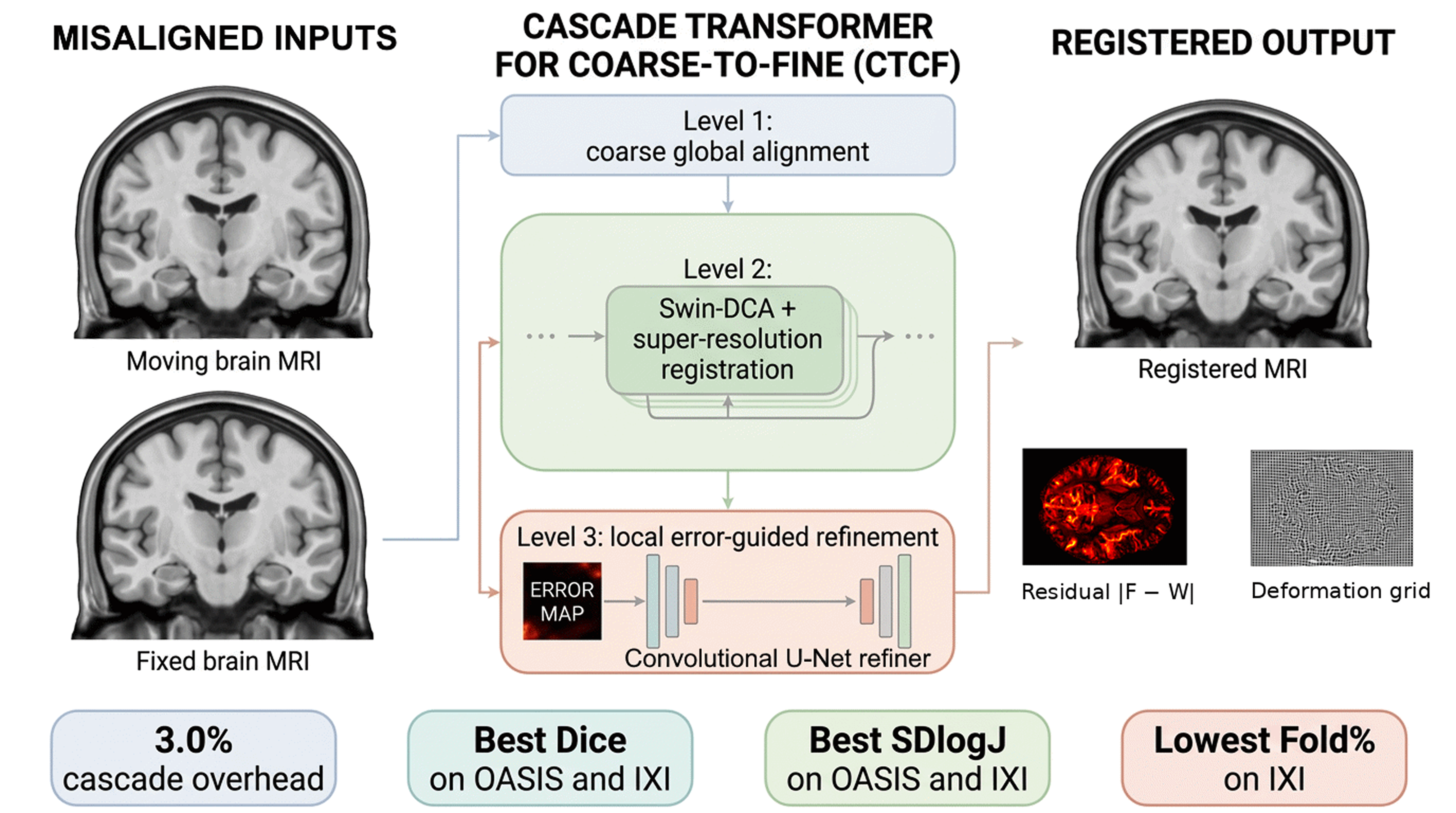
Deformable medical image registration aims to spatially align anatomical structures across volumetric scans. Recent transformer-based methods achieve high overlap accuracy but often produce deformation fields with topological violations. We propose CTCF, a Cascade Transformer for Coarse-to-Fine registration that wraps a lightweight coarse-and-refine envelope around a core registration module. Level 1 provides a coarse displacement estimate at quarter resolution, Level 2 performs the main registration via a Swin Transformer encoder with deformable cross-attention and a learned super-resolution decoder, and Level 3 applies error-driven flow refinement at half resolution. The two outer levels add only 3.0% parameter overhead yet improve registration accuracy while maintaining competitive deformation regularity relative to external baselines. The model is trained end-to-end with a composite unsupervised loss combining local normalized cross-correlation, diffusion regularization, inverse-consistency, and Jacobian-based topology preservation. On the OASIS brain MRI benchmark, CTCF achieves the highest Dice score of 0.8208 among the compared unsupervised methods while producing the lowest SDlogJ among the compared methods, with all Dice improvements statistically significant at p < 0.001 by the Wilcoxon signed-rank test. On IXI, CTCF also achieves the best Dice, HD95, SDlogJ, and fold percentage among the compared methods. A five-round ablation study validates each component: cascade decomposition isolates each level’s contribution, and resolution scaling experiments confirm the framework’s scalability, yielding further accuracy gains with zero parameter overhead.
Keywords:
deformable image registration
; unsupervised learning
; coarse-to-fine cascade
; Swin Transformer
; deformable cross-attention
; super-resolution decoding
; brain MRI registration
; health informatics
1. Introduction
Establishing dense spatial correspondences between volumetric medical images is central to many clinical and research workflows, from longitudinal brain atrophy monitoring to atlas-based segmentation propagation [1,2]. Deformable registration seeks a dense displacement field that warps one volume onto another while respecting anatomical plausibility, which imposes two competing demands: the field must be flexible enough to capture inter-subject variability yet smooth enough to avoid topological violations such as tissue folding [3,4].
Classical iterative optimization methods provide strong diffeomorphic guarantees but are prohibitively slow for large-scale studies. Convolutional neural networks (CNNs) address this bottleneck by predicting displacement fields in a single forward pass [5,6]. VoxelMorph [6] demonstrated that training with image similarity and smoothness objectives alone, without segmentation supervision, can yield competitive accuracy. Nonetheless, the limited effective receptive field of purely convolutional encoders constrains their capacity to resolve large or spatially heterogeneous deformations [7].
Vision transformers overcome this limitation through self-attention over patch tokens. TransMorph [7] paired a Swin Transformer encoder with a convolutional decoder and achieved substantial accuracy gains on brain MRI benchmarks. TransMorph-DCA [8] further replaced window-based self-attention with deformable cross-attention (DCA), allowing each encoder to selectively sample anatomically relevant tokens from the opposite image stream through learned offsets. This sparse adaptive sampling improves robustness to large deformations while keeping attention complexity comparable to the standard windowed variant. However, both methods still rely on convolutional decoders with interpolation-based upsampling, which may introduce aliasing artifacts and limit the spatial fidelity of the recovered displacement field.
An alternative line of work addresses the decoder bottleneck. UTSRMorph [9] recast displacement field reconstruction as a super-resolution (SR) problem, replacing trilinear interpolation with learned upsampling modules that progressively reconstruct high-resolution fields from coarse feature maps. The resulting deformation fields exhibit improved smoothness and spatial detail. Yet the encoder of UTSRMorph uses overlapping window self-attention rather than deformable cross-attention, which may limit the capacity for capturing sparse long-range correspondences between distant anatomical structures.
These two advances—deformable cross-attention and learned super-resolution—address complementary bottlenecks but remain single-pass architectures that must resolve global alignment and local detail simultaneously.
Coarse-to-fine decomposition has a long history in registration. Classical methods such as SyN [3] perform multi-resolution optimization, solving for large-scale deformations on downsampled grids before refining at finer scales. In the learning-based setting, Zhao et al. [10] proposed recursive cascaded networks that stack identical registration subnetworks, each refining the previous stage’s output, demonstrating that cascading improves accuracy on brain MRI. Mok and Chung [11] introduced LapIRN, which combines a Laplacian pyramid decomposition with multi-resolution registration to capture deformations at different spatial scales. However, both approaches replicate the same architecture at each level, resulting in proportional parameter growth with each added stage.
While these cascaded approaches demonstrate the value of multi-resolution decomposition, they share two limitations. First, they replicate a uniform architecture at every level, so each added stage incurs the full parameter and compute cost of the base network. Second, the refinement signal is implicit—later stages simply re-register warped images without an explicit measure of where the current alignment is deficient. Analogous benefits of stage-wise decomposition have been observed in other medical imaging tasks: for example, Nefediev et al. [12] reported that a cascaded pipeline combining prostate localization and subsequent segmentation improved prostate cancer segmentation on T2-weighted MRI, confirming that explicit stage decomposition is beneficial when a model must capture both global context and precise local boundaries. Additionally, topology-preserving constraints—inverse consistency, Jacobian penalties—are typically applied as auxiliary losses but are not tightly coupled with architectural design.
In this work, we propose CTCF (Cascade Transformer for Coarse-to-Fine registration), a three-level cascade framework that jointly addresses correspondence modeling, high-resolution deformation reconstruction, and topology-preserving regularization. Unlike single-pass methods, CTCF explicitly decomposes registration into three stages:
- Level 1: A lightweight convolutional network at quarter resolution that predicts a coarse displacement field, providing a global initialization for subsequent stages.
- Level 2: A Swin Transformer encoder with deformable cross-attention and a super-resolution decoder at half resolution, performing the main registration with iterative flow integration.
- Level 3: An error-driven convolutional refiner at half resolution that detects residual misalignment using local NCC error maps and predicts a corrective displacement update.
A smoothstep cascade warmup schedule progressively activates Level 1 and Level 3 during training, enabling stable optimization of the full cascade. The model is trained end-to-end with a composite unsupervised loss that enforces image similarity, deformation smoothness, inverse consistency, and topology preservation—no segmentation labels are used during training.
In our preliminary work [13], we presented an early version of CTCF with a single-stage refinement loop on OASIS. The present study extends this with an explicit three-level cascade, a stronger regularization strategy (inverse consistency + Jacobian penalty replacing cycle consistency), evaluation on both OASIS and IXI, and a five-round ablation study including cascade decomposition and resolution scaling.
The main contributions are:
- 1.
- A modular coarse-to-fine cascade (Levels 1 and 3) that adds only 3.0% parameter overhead to a Swin-DCA encoder with a learned super-resolution decoder. The cascade envelope is architecturally separable from the core module and, in principle, portable to alternative backbones.
- 2.
- An error-driven flow refinement module (Level 3) that uses per-voxel local NCC error maps to detect and correct residual misalignment, validated against two alternative error formulations.
2. Materials and Methods
2.1. Problem Formulation
Given a moving image and a fixed image defined on a discrete spatial domain , we estimate a dense displacement field defined on the fixed-image grid. The associated sampling transformation is
We denote spatial warping by , defined as
where trilinear interpolation is used whenever falls at a non-integer location. The goal of deformable registration is to estimate such that .
2.2. Architecture Overview
CTCF is a three-level cascade operating at multiple spatial resolutions (Figure 1). The design assigns a distinct role to each level: Level 1 captures large-scale global alignment at low cost, Level 2 performs the main dense registration with full model capacity, and Level 3 corrects residual local errors using an explicit quality signal. This separation allows each level to specialize for a particular spatial scale of deformation, rather than forcing a single network to simultaneously estimate both coarse and fine displacements.
Given input volumes of size , Level 1 predicts a coarse flow at resolution (), Level 2 performs the main Swin-DCA registration with iterative flow integration at resolution (), and Level 3 applies error-driven refinement at resolution. All levels output at half resolution; the final composite flow is upsampled to full resolution via trilinear interpolation with magnitude scaling.
2.3. Level 1: Coarse Flow Predictor
Level 1 is a lightweight convolutional U-Net operating at quarter resolution (), shown in Figure 1 (left) with internal structure detailed in Figure 2(b). The moving and fixed images are downsampled by via trilinear interpolation and concatenated along the channel dimension to form a 2-channel input.
The network consists of two encoder stages, a bottleneck, and two decoder stages with skip connections. Each stage applies a convolutional block:
where denotes LeakyReLU () and IN denotes instance normalization [14]. Encoder stages are connected by average pooling; decoder stages use trilinear upsampling with skip connections.
The bottleneck is augmented with two dilated residual context blocks with dilation rates 1 and 2, respectively. Each context block applies two convolutions (the first with the specified dilation rate) with a residual connection scaled by a factor of :
where d denotes the dilation rate and the second convolution of each block is zero-initialized to ensure identity-like behavior at the start of training.
The output layer ( convolution producing 3-channel flow) is also zero-initialized, so the coarse flow starts as the identity transformation and gradually learns meaningful displacements during training. The predicted quarter-resolution flow is upsampled by to half resolution via trilinear interpolation with proportional magnitude scaling, and modulated by the cascade weight :
Level 1 uses base channels (encoder stages: , bottleneck: 128), totaling 3.19M parameters. It captures large-scale global deformations, providing an effective initialization that reduces the residual deformation Level 2 must model.
2.4. Level 2: Swin-DCA Encoder with SR Decoder
Level 2 is the main registration module, operating at half resolution (). It combines a dual-stream Swin Transformer encoder with deformable cross-attention (DCA) from TransMorph-DCA [8] and a learned upsampling decoder inspired by the super-resolution (SR) paradigm of UTSRMorph [9].
2.4.1. Patch Embedding
Each half-resolution input image ( or ) is partitioned into non-overlapping patches () and projected into a C-dimensional token embedding via a learnable linear layer:
where is the number of patches and is the embedding dimension. Relative position encoding (RPE) is added to the attention computation to inject spatial inductive bias [15].
2.4.2. Dual-Stream Encoder with Deformable Cross-Attention
The encoder processes the moving and fixed token sequences through two parallel streams across hierarchical stages with depths transformer blocks per stage and 8 attention heads. Between stages, patch merging layers downsample tokens by and double the channel dimension, yielding feature maps at resolutions , , and of the half-resolution input.
Within each transformer block, window-based self-attention (W-MSA) captures intra-image spatial relationships within local windows of size at the three respective stages. Deformable cross-attention (DCA) [8], illustrated in Figure 2(a), then enables inter-image feature exchange. Unlike standard windowed cross-attention which uses rectangular windows of identical shape for both images, DCA employs a lightweight offset network to learn per-head sampling offsets that deform the window partition of the reference stream:
where and denote the base and reference token streams, WP denotes window partition, samples tokens at shifted positions via trilinear interpolation, and is the per-head dimension. The offset network consists of a depth-wise convolution followed by layer normalization, GeLU activation, and a pointwise convolution. Deformable window sizes are set to at the three stages, providing progressively finer-grained cross-image correspondence as the feature resolution decreases. Within each block, both streams are updated simultaneously: each stream serves as both query source and key/value provider, using two independent offset networks (Figure 2(a)).
At each encoder level l, features from both streams are fused by element-wise summation and refined by a channel attention block (CAB):
The CAB consists of two convolutions with a GELU activation, followed by a squeeze-and-excitation channel attention module [16] with compression ratio 3 and squeeze factor 30:
where is the convolutional body, GAP denotes global average pooling, FC are fully connected layers, is the sigmoid function, and ⊙ denotes channel-wise multiplication.
2.4.3. Learned Upsampling Decoder
The decoder progressively reconstructs half-resolution deformation features from the deepest encoder features. Instead of interpolation-based upsampling, we employ SR-style upsampling blocks (Figure 2(c)) that increase spatial resolution by via trilinear interpolation followed by two convolutional refinement layers ( convolutions with GELU activation):
where s denotes the skip connection from the corresponding encoder level and is trilinear upsampling. Both transformer-level skip connections (from CAB outputs at each encoder stage) and convolution-level skip connections (from a shallow convolutional feature extractor applied to the concatenated half-resolution inputs) propagate multi-scale spatial information to the decoder.
Three SR upsampling blocks progressively increase the resolution from to , , and of the half-resolution input, yielding a feature map at the full half-resolution grid.
2.4.4. Iterative Flow Integration
The decoded features are refined through integration steps (validated in Section 3.1, Round 2). Each step t has its own independently parameterized context extractor, SR upsampling block, and registration head (weights are not shared across steps), enabling specialization for different stages of flow refinement.
At each step t, the current deformation estimate warps the moving image to produce an intermediate aligned image . A context module (Conv3d with ReLU) extracts appearance discrepancies between and , which are combined with the decoder features via an SR upsampling block and passed to a registration head (a single convolution) that predicts an incremental flow update . The flow is updated via differentiable displacement composition:
Here, denotes channel-wise trilinear resampling of the incremental displacement field at locations , and .
If Level 1 provides an initial flow , this is used to initialize and pre-warp the moving image before the first integration step. This warm-starting mechanism allows Level 2 to focus on residual deformations rather than re-estimating the global displacement from scratch.
Level 2 constitutes 287.11M parameters and is the dominant computational component. The half-resolution operating point follows the design of TransMorph-DCA [8], which originally introduced processing at input resolution to reduce the quadratic memory cost of windowed self-attention while preserving registration accuracy.
2.5. Level 3: Error-Driven Flow Refiner
Level 3 is a convolutional U-Net (Figure 2(b)) that refines the flow from Level 2 by detecting and correcting residual misalignment. It receives four inputs concatenated along the channel dimension: (1) the warped moving image , (2) the fixed image , (3) an error map E, and (4) the current flow field —totaling 6 input channels.
2.5.1. Error Map Computation
The error map quantifies local registration quality, providing an explicit spatial signal indicating where the current alignment is deficient. We use the local NCC error:
where is the squared local normalized cross-correlation computed with a window of size . This error map takes values in , where 0 indicates perfect local alignment and 1 indicates no correlation. Unlike simpler alternatives such as absolute intensity difference or gradient magnitude difference, the NCC-based error captures structural misalignment invariant to local intensity contrast. The NCC computation is forced to float32 precision regardless of the training mixed-precision mode to avoid catastrophic cancellation in the windowed sums ( taps). The error map is computed under gradient detachment (torch.no_grad), providing an informative spatial signal to the refiner without adding to the computational graph.
2.5.2. Refinement Network
The refiner follows the same U-Net architecture as Level 1 (Eq. 3): two encoder stages with average pooling, a bottleneck (without context blocks), and two decoder stages with skip connections. It uses base channels (encoder stages: , bottleneck: 256), totaling 5.66M parameters. The output layer is zero-initialized, so the refiner initially predicts and progressively learns to apply corrections only where needed.
The residual flow is scaled by and added to the Level 2 flow:
The lightweight convolutional refiner complements the transformer encoder, which excels at global correspondences but may not resolve fine-grained local misalignments in structurally complex regions such as cortical folds.
Together, Levels 1 and 3 add 8.85M parameters (3.19M + 5.66M), constituting only 3.0% of the total model size (295.96M). This small overhead is important for fair comparison: the cascade levels are deliberately kept lightweight so that any performance improvement is consistent with the benefit of the proposed full design, which combines cascade decomposition with the chosen decoder and training recipe, rather than with additional model capacity.
2.6. Final Output
The composite half-resolution flow is upsampled to full resolution using trilinear interpolation with magnitude scaling:
The warped output is , obtained by applying the full-resolution displacement field to the moving image via differentiable spatial transformation (Eq. 2).
2.7. Cascade Warmup Schedule
Training the full three-level cascade from the start can lead to instability, as Level 2 has not yet learned meaningful features when Levels 1 and 3 begin contributing. We introduce a smoothstep warmup schedule that gradually activates the outer cascade levels.
The cascade weights , , and the global warmup factor w ramp from 0 to 1 over epochs using a smoothstep function:
where and , with denoting the total number of training epochs. During the initial 5% of training, only Level 2 is active, allowing it to establish a stable feature representation before the coarse and refinement levels are introduced.
2.8. Loss Function
CTCF is trained bidirectionally: for each pair , both the forward registration () and backward registration () are computed within each training iteration. All loss terms are computed symmetrically and averaged. The total loss is:
The image similarity loss is the local normalized cross-correlation (NCC) with window size [6], computed on full-resolution warped images:
where denotes the local neighborhood and the local mean. The diffusion regularization penalizes spatial gradients of the displacement field to encourage smoothness [6]:
The inverse-consistency loss (ICON) enforces approximate invertibility via displacement composition [17]. Given forward and backward displacement fields and , with associated sampling transforms and :
where denotes the mean absolute value; ideally , meaning . Finally, the Jacobian determinant penalty discourages topological foldings [4]. The Jacobian matrix of the sampling transformation is , and the penalty is:
The default loss weights are (OASIS) / (IXI), , .
2.9. Experimental Setup
2.9.1. Datasets
The OASIS brain MRI dataset [18] contains 414 T1-weighted 3D volumes with anatomical segmentations covering 35 cortical and subcortical regions. Following the standard protocol [7], we split the data into 394 training and 19 test volumes, with one designated atlas volume used as the fixed image for all test pairs. Consistent with prior work [6,7], the best checkpoint is selected based on atlas-pair Dice used for model selection. Because the standard OASIS protocol does not define a separate validation split, these results should be interpreted as following the established benchmark protocol rather than as a strictly held-out test estimate. All volumes are preprocessed to a fixed spatial size of with per-volume intensity normalization. During training, moving–fixed pairs are formed as unordered pairs sampled from the training set.
The IXI dataset contains T1-weighted brain MRI volumes from healthy subjects. Following the protocol of [7], we use 576 volumes split into 403 for training, 58 for validation, and 115 for testing. The best checkpoint is selected based on validation Dice on the 58 validation subjects; final evaluation is performed on the 115 test subjects, which are not used during training or checkpoint selection. Volumes are preprocessed to with 30 anatomical label regions for evaluation.
2.9.2. Evaluation Metrics
- Dice Similarity Coefficient (DSC): computed between warped moving and fixed segmentations, averaged over all anatomical labels (35 for OASIS, 30 for IXI).
- Standard Deviation of (SDlogJ): measures deformation regularity, where lower values indicate smoother fields.
- Folding Percentage: proportion of voxels with , indicating topological violations.
- 95th Percentile Hausdorff Distance (HD95): captures boundary alignment accuracy.
For methods operating at reduced resolution, the displacement field is upsampled to full resolution with magnitude scaling consistent with the downsampling factor before evaluation.
2.9.3. Baseline Methods
We compare CTCF against two recent transformer-based registration methods:
- 1.
- TransMorph-DCA [8]: extends TransMorph with deformable cross-attention for sparse adaptive correspondence modeling. Trained with NCC and diffusion regularization in an unsupervised setting.
- 2.
- UTSRMorph [9]: formulates displacement prediction as a super-resolution problem with learned upsampling modules. Uses a Swin Transformer encoder with window-based self-attention.
Both baselines are trained and evaluated using the original authors’ publicly released codebases, ensuring that the comparison reflects the published architectures and training procedures. For UTSRMorph, we use the Large configuration (embedding dimension 160, 421.50M parameters), which is larger than the base variant reported in the original paper (embedding dimension 48); this choice provides a stronger baseline for comparison. All methods use the same data splits, preprocessing, and evaluation protocol. For OASIS, all models use and . For IXI, UTSRMorph uses and following its original protocol [9]; CTCF and TransMorph-DCA use with (IXI).
2.9.4. Implementation Details
All models are implemented in PyTorch and trained for 500 epochs using AdamW with batch size 1. CTCF uses a learning-rate schedule consisting of a constant rate during the cascade warmup phase (first 15% of epochs), followed by polynomial decay (power 0.9, minimum ). Baseline methods use polynomial decay from epoch 0. Automatic mixed precision (AMP) is used to reduce memory consumption. TransMorph-DCA and CTCF operate at half resolution during training (inputs downsampled by via trilinear interpolation), following the half-resolution design introduced in the TransMorph-DCA codebase [8], with final flow upsampled by for evaluation. UTSRMorph predicts the full-resolution flow in a single forward pass.
The loss functions differ across methods: both baselines use NCC + diffusion regularization only. All methods are trained with their original loss configurations to ensure the comparison reflects the published recipes.
CTCF is trained bidirectionally: both forward () and backward () registrations are computed within each iteration. TransMorph-DCA and UTSRMorph are trained unidirectionally in their original codebases; the bidirectional protocol used for CTCF provides additional regularization through symmetric loss computation (Section 2.8), which may contribute to the observed deformation smoothness.
Training was performed on a single NVIDIA RTX PRO 6000 Blackwell GPU 96 GB.
3. Results
3.1. Ablation Study
We conducted a systematic ablation study organized in five rounds to validate each architectural component. Each round builds on the best configuration identified in the preceding round, following a greedy sequential design. All ablation experiments were trained for 100 epochs on the OASIS dataset with otherwise identical hyperparameters (learning rate , , , ). The 100-epoch budget is sufficient for configuration ranking: the relative ordering of methods is stable well before convergence, as confirmed by the final 500-epoch runs which preserve the same ranking.
3.1.1. Round 1: Loss and Strategy Variants
Round 1 started from the initial CTCF configuration and evaluated five variants of the loss function and cascade activation strategy. Switching the ICON penalty from L1 to L2 norm substantially improved regularity (SDlogJ 0.069, Fold 0.07%) but at a significant Dice cost (−0.004), indicating that the L2 penalty over-regularizes the displacement field. Prealignment of the Level 2 encoder input (warping the moving image by the Level 1 flow before encoding) and early Level 1 activation (bypassing the cascade warmup) both showed no significant benefit, suggesting that the warmup schedule adequately handles the Level 1 integration.
3.1.2. Round 2: Level 3 and Integration Tuning
Round 2 focused on the error-driven refiner and the iterative integration module. Increasing the Level 3 base channels from 32 to 64 and adopting the NCC error mode yielded the largest single improvement across all rounds (+0.0053 Dice over the Round 1 best). Reducing the number of integration steps from 12 to 6 maintained accuracy while halving the integration overhead, confirming that 6 steps provide sufficient flow refinement for this resolution. Swin-specific tuning (drop path rate 0.1, learnable QKV bias) degraded performance (−0.0008), indicating that the performance bottleneck lies in the cascade and decoder design rather than the encoder configuration.
3.1.3. Round 3: Level 1 Capacity
Round 3 optimized the coarse predictor capacity by comparing 32 and 64 base channels. The smaller configuration (32 channels, 3.19M parameters) outperformed the larger one (64 channels, 12.63M parameters) with Dice 0.8162 vs. 0.8155. This indicates that Level 1’s role is to provide a rough global initialization, not to model fine-grained deformations; excess capacity leads to overfitting at the coarse scale without benefiting downstream levels.
3.1.4. Round 4: Cascade Decomposition
To isolate the independent contribution of each cascade level, we trained three reduced configurations: Level 2 only (core module without cascade), Level 1 + Level 2 (coarse initialization only), and Level 2 + Level 3 (refinement only). The full CTCF (Round 3 best) serves as the reference.
Level 2 alone achieves Dice 0.8036. Adding Level 1 yields a negligible improvement (+0.0001), indicating that the coarse predictor provides minimal direct benefit to Level 2 in isolation. However, Level 3 dramatically improves performance: L2+L3 achieves 0.8148 (+0.0112 over L2 alone), confirming that error-driven refinement is the primary contributor. The full cascade (L1+L2+L3) reaches 0.8162, gaining an additional +0.0014 over L2+L3. This reveals a synergistic effect: Level 1’s coarse initialization provides a better starting flow for Level 3, improving the refiner’s ability to detect and correct residual errors.
Deformation regularity shows another pattern. Level 2 alone and L1+L2 produce very smooth fields (Fold %), while configurations including Level 3 show Fold %. This trade-off is inherent to the refiner’s role: Level 3 introduces additional deformation flexibility to correct alignment errors, which locally creates folds. The net effect—substantially higher Dice with controlled fold percentage—validates the cascade design.
Table 1 summarizes the key ablation results across Rounds 1–4.
Figure 3 provides a visual summary of the ablation results across Rounds 1–4.
3.1.5. Round 5: Resolution Scaling
To assess the untapped capacity of the cascade, we raised the operating resolution: Level 1 to half () and Level 3 to full (), using the same architectures with zero additional parameters. On top of this base, we tested iterative L3 refinement (two shared-weight passes, +0 params), learned convex upsampling (+5K), an L2→L3 skip connection (+83K), and a combined variant (+88K, 0.03% overhead).
All Round 5 configurations achieve Dice 0.831–0.833 (+0.015–0.017 over the R3 reference), with a spread of only 0.0018, confirming that the resolution upgrade—not individual enhancements—is the dominant factor (Table 2, Figure 4). The cost is higher GPU memory (53–83 GB vs. GB at the standard resolution; an iterative L3 variant with three passes exceeded 96 GB and was infeasible) and moderate regularity degradation: SDlogJ rises from 0.080 to ∼0.086 (+8%), fold % from 0.33 to ∼0.45 (+36%). The degraded SDlogJ still substantially outperforms UTSRMorph (0.1015), and the regularization weights were not retuned, suggesting the tradeoff is manageable. Overall, Round 5 demonstrates that the cascade has substantial untapped capacity: removing the resolution constraint yields +0.016 Dice with zero parameter overhead.
Figure 4 provides a visual comparison of the Round 5 configurations.
3.2. Main Comparison
The ablation study identified the optimal CTCF configuration: Level 1 with 32 base channels at quarter resolution, Level 2 with 6 integration steps, and Level 3 with 64 base channels using the NCC error mode at half resolution. This configuration was trained for the full 500 epochs on both OASIS and IXI alongside the two baselines under identical evaluation protocols. The 500-epoch runs preserve the same relative ranking observed at 100 epochs, confirming the validity of the ablation protocol.
Table 3 presents the quantitative comparison on the OASIS evaluation set ( pairs, per the standard protocol [7]). CTCF achieves the best performance on Dice, HD95, and SDlogJ. The improvement in deformation regularity over UTSRMorph is particularly pronounced: SDlogJ is reduced by 21.5%, despite CTCF operating at half resolution. TransMorph-DCA achieves the lowest fold percentage (0.264%), as its single-pass architecture avoids the additional local deformation introduced by Level 3 refinement. CTCF’s ICON and Jacobian penalties constrain the fold rate (0.523% vs. 0.890% for UTSRMorph), but cannot fully offset the extra flexibility of the cascade refiner—a tradeoff validated in Round 4. Statistical significance is confirmed in Section 3.5.
Table 4 reports the IXI results ( test subjects). CTCF outperforms both baselines on all metrics, again demonstrating the regularizing effect of the cascade decomposition.
3.3. Training Dynamics
Figure 5 shows the validation Dice convergence curves on both datasets. All three models converge within the first 50–100 epochs, with CTCF establishing a consistent lead after the cascade warmup phase (epochs 25–75). On IXI, CTCF reaches 0.7607 Dice by epoch 102 and plateaus, surpassing both baselines trained for 500 epochs. The smoothstep cascade schedule (Eq. 17) gradually activates Levels 1 and 3 between epochs 25 and 75.
Each CTCF training epoch takes approximately 2.7 minutes before cascade activation and 3.3 minutes afterward, with peak GPU memory rising from GB to GB as Levels 1 and 3 become active. The full 500-epoch OASIS run completes in approximately 27 hours on the training hardware described in Section 2.9.4. Note that CTCF is trained bidirectionally (two forward passes per iteration), which accounts for part of this cost relative to single-pass baselines.
3.4. Per-Case and Per-Region Analysis
Figure 6 shows the per-case Dice distributions on both datasets. CTCF exhibits a higher median, a tighter interquartile range, and fewer low-Dice outliers on both datasets.
Figure 7 presents the per-region Dice analysis across all 35 anatomical regions, sorted by inter-method variance to highlight regions where methods diverge most. CTCF consistently achieves the highest or near-highest Dice across all regions, with the largest advantages observed in structurally complex areas such as the hippocampus, amygdala, and ventral diencephalon.
Figure 7.
Per-region Dice scores on OASIS for all methods across 35 anatomical regions, sorted by inter-method variance. Regions with the largest performance differences are shown on the left.
Figure 7.
Per-region Dice scores on OASIS for all methods across 35 anatomical regions, sorted by inter-method variance. Regions with the largest performance differences are shown on the left.

Figure 8.
Per-region Dice advantage of CTCF over baselines on OASIS. Positive values indicate regions where CTCF outperforms the respective baseline.
Figure 8.
Per-region Dice advantage of CTCF over baselines on OASIS. Positive values indicate regions where CTCF outperforms the respective baseline.

Figure 9 presents the analogous per-region analysis on IXI across all 30 anatomical regions. CTCF achieves the highest or near-highest Dice across the majority of regions, with the largest advantages in subcortical structures. Figure 10 highlights the per-region Dice advantage of CTCF over both baselines.
3.5. Statistical Analysis
We assess the statistical significance of performance differences between CTCF and each baseline using the Wilcoxon signed-rank test on paired per-case metrics. Effect sizes are quantified via the Hodges–Lehmann estimator (median of all pairwise averages of paired differences) with 95% confidence intervals. Detailed results are reported in Table 5 and Table 6. In both tables, significance levels are: * , ** , *** , ns = not significant; negative HL values for HD95, SDlogJ, and Fold% indicate that CTCF is better (lower).
On OASIS (, exact Wilcoxon test), CTCF significantly outperforms both baselines on Dice (; Hodges–Lehmann: vs. TM-DCA, vs. UTSRMorph). For HD95, CTCF is significantly better than TM-DCA (, HL ) and UTSRMorph (, HL ). For deformation regularity, CTCF achieves dramatically lower SDlogJ than UTSRMorph (, HL ), while the difference with TM-DCA is not statistically significant (), reflecting the shared half-resolution operating point and Swin-DCA encoder.
On IXI (, approximate Wilcoxon test), all pairwise differences are statistically significant (). CTCF outperforms TM-DCA by a large margin on Dice (HL ), HD95 (HL ), and fold percentage (HL pp). Against UTSRMorph, CTCF yields a smaller but significant Dice advantage (HL ) with substantially better HD95 (HL ) and fold percentage (HL pp). Notably, CTCF achieves the best SDlogJ (0.0594) among all methods on this dataset, surpassing both UTSRMorph (0.0627) and TM-DCA (0.0874).
3.6. Qualitative Comparison
Figure 11 and Figure 12 present qualitative comparisons on representative test cases from OASIS and IXI. Each figure shows checkerboard overlays (alignment quality), residual error maps (darker = better), and deformed grids (deformation smoothness) for all three methods.
On OASIS (Figure 11), CTCF produces the lowest residual error and the smoothest deformation grid, consistent with its quantitative SDlogJ advantage. UTSRMorph achieves comparable alignment but with visibly more irregular deformations. On IXI (Figure 12), the CTCF grid remains smooth throughout, while TM-DCA exhibits substantial folding artifacts consistent with its 2× higher fold percentage.
3.7. Parameter Efficiency
Table 7 summarizes model complexity and key metrics on OASIS. CTCF achieves the best Dice and SDlogJ with 30% fewer parameters than UTSRMorph-Large (295.96M vs. 421.50M) and only 4.2% more than TransMorph-DCA (283.93M). The cascade overhead totals 8.85M parameters (3.19M + 5.66M), constituting only 3.0% of the total model.
4. Discussion
4.0.1. Cascade as Architectural Contribution
TransMorph-DCA provides a closely related transformer baseline sharing the Swin-DCA encoder, which helps isolate the cascade’s contribution beyond what additional capacity could explain: despite minimal parameter overhead (Section 3.7), the cascade produces statistically significant improvements in Dice and HD95 (Table 5). The cascade decomposition (Round 4) further reveals that Level 1’s value is indirect: it contributes negligibly in isolation but improves Level 3’s effectiveness by providing coarse initialization, a synergistic effect that single-pass architectures cannot exploit.
4.0.2. Deformation Regularity
CTCF reduces SDlogJ by 21.5% relative to UTSRMorph (), attributable to two complementary mechanisms: the half-resolution operating point, which limits the spatial frequency of the predicted displacement, and the cascade decomposition, which distributes the deformation across three levels. That SDlogJ is comparable between CTCF and TM-DCA () while Dice is significantly higher confirms that the cascade improves accuracy without compromising regularity.
4.0.3. Error-Driven Refinement
Level 3 accounts for 89% of the total cascade Dice gain (Round 4), making error-driven refinement the dominant mechanism. The NCC error mode outperforms alternatives because it captures structural misalignment invariant to local intensity contrast. Combined with zero-initialized output, this ensures the refiner applies corrections only where the error signal warrants it, functioning as a learned residual connection.
4.0.4. Resolution Tradeoff and Scalability
Despite operating at fewer voxels than UTSRMorph, CTCF outperforms it on all metrics on both datasets (Table 3Table 4), suggesting that the coarse-to-fine decomposition compensates for reduced resolution by capturing deformations at appropriate spatial scales. Round 5 confirms the cascade has untapped capacity: higher-resolution Levels 1 and 3 yield +0.016 Dice with zero parameter overhead, at the cost of increased GPU memory (53–83 GB) and moderate SDlogJ degradation (+8%, without retuning regularization weights).
4.0.5. Comparison with Preliminary Work
Relative to our preliminary conference paper [13], this work introduces the three-level cascade (Levels 1 and 3 are new), replaces cycle-consistency loss with inverse-consistency and Jacobian penalties, adds systematic ablation across five rounds of experiments including cascade decomposition and resolution scaling studies, and provides rigorous statistical comparison against baselines using original codebases under identical data splits, preprocessing, and evaluation settings, while retaining method-specific published training recipes.
4.0.6. Limitations
- 1.
- Level 2 inherits the computational cost of the Swin-DCA encoder (287.11M parameters); replacing it with a more efficient backbone would make the cascade more practical.
- 2.
- The fixed three-level structure does not adapt to registration difficulty; skipping Level 3 in easy regions could improve efficiency.
- 3.
- Higher-resolution operation (Round 5) requires 53–83 GB GPU memory, limiting practical deployment.
- 4.
- Evaluation is limited to brain MRI on two datasets; generalization to other anatomies and modalities remains to be validated.
- 5.
- For OASIS, model selection follows the standard atlas-pair protocol and therefore uses the same 19 evaluation pairs for checkpoint selection, since no separate validation split is defined. This may yield somewhat optimistic OASIS estimates relative to a fully held-out evaluation; the IXI results provide the cleaner validation/test separation.
5. Conclusions
We presented CTCF, a three-level coarse-to-fine cascade for unsupervised 3D brain MRI registration. The cascade adds only 3.0% parameter overhead over the core Swin-DCA module, yet achieves statistically significant Dice improvements on both OASIS and IXI, with the smoothest deformation fields among the compared methods. A five-round ablation study validated each component, identified the optimal configuration, and demonstrated via resolution scaling that the framework has substantial untapped capacity (+0.016 Dice at higher resolution with zero extra parameters).
Future work includes evaluating the cascade envelope with alternative encoder architectures, topology-preserving refinement for regularity at higher resolution, and validation on additional anatomies and modalities.
Author Contributions
Conceptualization, D.P. and R.D.; methodology, D.P.; software, D.P.; validation, D.P.; formal analysis, D.P.; investigation, D.P. and R.D.; resources, R.D.; writing—original draft preparation, D.P.; writing—review and editing, D.P. and R.D.; visualization, D.P.; supervision, R.D.; project administration, R.D.; funding acquisition, R.D. All authors have read and agreed to the published version of the manuscript.
Funding
This research received no external funding.
Institutional Review Board Statement
Not applicable.
Informed Consent Statement
Not applicable.
Data Availability Statement
The OASIS dataset is publicly available at https://www.oasis-brains.org. The IXI dataset is publicly available at https://brain-development.org/ixi-dataset/. The source code is publicly available at https://github.com/Palllladium/CTCF.
Acknowledgments
During the preparation of this manuscript, the authors used Claude (https://www.anthropic.com, Anthropic) for the purposes of language refinement, grammar correction, academic tone enhancement, and manuscript formatting. The Graphical Abstract draft was created using Nano Banana 2 (https://deepmind.google, Google). The authors have reviewed and edited all output and take full responsibility for the content of this publication.
Conflicts of Interest
The authors declare no conflicts of interest.
Abbreviations
The following abbreviations are used in this manuscript:
| CTCF | Cascade Transformer for Coarse-to-Fine registration |
| DCA | Deformable Cross-Attention |
| SR | Super-Resolution |
| NCC | Normalized Cross-Correlation |
| DSC | Dice Similarity Coefficient |
| SDlogJ | Standard Deviation of |
| HD95 | 95th percentile Hausdorff Distance |
| ICON | Inverse Consistency |
| MRI | Magnetic Resonance Imaging |
References
- Sotiras, A.; Davatzikos, C.; Paragios, N. Deformable medical image registration: A survey. IEEE Trans. Med. Imaging 2013, 32, 1153–1190. [Google Scholar] [CrossRef] [PubMed]
- Hill, D.L.G.; Batchelor, P.G.; Holden, M.; Hawkes, D.J. Medical image registration. Phys. Med. Biol. 2001, 46, R1–R45. [Google Scholar] [CrossRef] [PubMed]
- Avants, B.B.; Epstein, C.L.; Grossman, M.; Gee, J.C. Symmetric diffeomorphic image registration with cross-correlation: Evaluating automated labeling of elderly and neurodegenerative brain. Med. Image Anal. 2008, 12, 26–41. [Google Scholar] [CrossRef] [PubMed]
- Dalca, A.V.; Balakrishnan, G.; Guttag, J.; Sabuncu, M.R. Unsupervised learning of probabilistic diffeomorphic registration for images and surfaces. Med. Image Anal. 2019, 57, 226–236. [Google Scholar] [CrossRef] [PubMed]
- Balakrishnan, G.; Zhao, A.; Sabuncu, M.R.; Guttag, J.; Dalca, A.V. An unsupervised learning model for deformable medical image registration. In Proceedings of the IEEE/CVF Conf. Computer Vision and Pattern Recognition (CVPR), Salt Lake City, UT, USA, 18–22 June 2018; pp. 9252–9260. [Google Scholar]
- Balakrishnan, G.; Zhao, A.; Sabuncu, M.R.; Guttag, J.; Dalca, A.V. VoxelMorph: A learning framework for deformable medical image registration. IEEE Trans. Med. Imaging 2019, 38, 1788–1800. [Google Scholar] [CrossRef] [PubMed]
- Chen, J.; Frey, E.C.; He, Y.; Segars, W.P.; Li, Y.; Du, Y. TransMorph: Transformer for unsupervised medical image registration. Med. Image Anal. 2022, 82, 102615. [Google Scholar] [CrossRef] [PubMed]
- Chen, J.; Liu, Y.; He, Y.; Du, Y. Deformable Cross-Attention Transformer for Medical Image Registration. In Machine Learning in Medical Imaging (MLMI 2023), Proceedings of the 14th International Workshop Lecture Notes in Computer Science; Vancouver, BC, Canada, Springer: Cham, Switzerland, 8 October 2023; Volume 14348, pp. 115–125. [Google Scholar] [CrossRef]
- Zheng, Y.; Wang, Z.; Huang, B.; Lim, N.H.; Papież, B.W. UTSRMorph: Unified transformer and super-resolution framework for unsupervised deformable medical image registration. IEEE Trans. Med. Imaging 2025, 44, 902–916. [Google Scholar]
- Zhao, S.; Dong, Y.; Chang, E.I.-C.; Xu, Y. Recursive Cascaded Networks for Unsupervised Medical Image Registration. In Proceedings of the IEEE/CVF International Conference on Computer Vision (ICCV), Seoul, Republic of Korea, 27 October–2 November 2019; pp. 10600–10610. [Google Scholar] [CrossRef]
- Mok, T.C.W.; Chung, A.C.S. Large Deformation Diffeomorphic Image Registration with Laplacian Pyramid Networks. In Medical Image Computing and Computer Assisted Intervention (MICCAI 2020), Proceedings of the 23rd International Conference Lecture Notes in Computer Science, Lima, Peru, 4–8 October 2020; Springer: Cham, Switzerland, 2020; Volume 12263, pp. 211–221. [Google Scholar] [CrossRef]
- Nefediev, N.; Staroverov, N.; Davydov, R. Improving Prostate Cancer Segmentation on T2-Weighted MRI Using Prostate Detection and Cascaded Networks. Algorithms 2026, 19, 85. [Google Scholar] [CrossRef]
- Pasenko, D.V. CTCF: Cascaded Transformer with Cross-Attention and Super-Resolution for Unsupervised Medical Image Registration. In Proceedings of the 2026 ElCon Conference of Young Researchers (ElCon-CN), Saint Petersburg, Russia, 3–5 February 2026; pp. 120–127. [Google Scholar] [CrossRef]
- Ulyanov, D.; Vedaldi, A.; Lempitsky, V. Instance normalization: The missing ingredient for fast stylization. arXiv 2016, arXiv:1607.08022. [Google Scholar]
- Liu, Z.; Lin, Y.; Cao, Y.; Hu, H.; Wei, Y.; Zhang, Z.; Lin, S.; Guo, B. Swin Transformer: Hierarchical vision transformer using shifted windows. In Proceedings of the IEEE/CVF Int. Conf. Computer Vision (ICCV), Montreal, QC, Canada, 11–17 October 2021; pp. 9992–10002. [Google Scholar]
- Hu, J.; Shen, L.; Sun, G. Squeeze-and-excitation networks. In Proceedings of the IEEE/CVF Conf. Computer Vision and Pattern Recognition (CVPR), Salt Lake City, UT, USA, 18–22 June 2018; pp. 7132–7141. [Google Scholar]
- Zhang, J. Inverse-consistent deep networks for unsupervised deformable image registration. arXiv 2018, arXiv:1809.03443. [Google Scholar] [CrossRef]
- Marcus, D.S.; Wang, T.H.; Parker, J.; Csernansky, J.G.; Morris, J.C.; Buckner, R.L. Open Access Series of Imaging Studies (OASIS): Cross-sectional MRI data in young, middle-aged, nondemented, and demented older adults. J. Cogn. Neurosci. 2007, 19, 1498–1507. [Google Scholar] [CrossRef] [PubMed]
Figure 1.
Overall three-level cascade architecture of the proposed CTCF (Cascade Transformer for Coarse-to-Fine) framework. Level 1 predicts a coarse displacement field at quarter resolution, Level 2 performs the main registration via a dual-stream Swin Transformer encoder with deformable cross-attention (DCA) and a learned super-resolution decoder with iterative flow integration at half resolution, and Level 3 refines the displacement field using an error-driven convolutional U-Net. The legend defines all module types, operators, and arrow styles used throughout Figure 1 and Figure 2.

Figure 2.
Architectural details of CTCF building blocks. (a) Symmetric dual-stream Swin-DCA block with independent offset networks and residual connections. (b) Convolutional U-Net template shared by Level 1 and Level 3 (with per-level channel configuration). (c) Super-resolution (SR) upsampling block with skip connection.

Figure 3.
Visual summary of ablation results on OASIS (100 epochs, Rounds 1–4). Bar chart showing Best Dice, SDlogJ, and Fold % across all configurations, color-coded by ablation round (R1: loss/strategy, R2: decoder tuning, R3: Level 1 capacity, R4: cascade decomposition). The best configuration (R3: L1=32, L3=64, TS6) is highlighted.

Figure 4.
Round 5 resolution scaling results on OASIS (100 epochs). Bar chart showing Best Dice, SDlogJ, and Fold % for each R5 configuration with the R3 reference.
Figure 4.
Round 5 resolution scaling results on OASIS (100 epochs). Bar chart showing Best Dice, SDlogJ, and Fold % for each R5 configuration with the R3 reference.

Figure 5.
Validation Dice vs. epoch on OASIS (left, 500 epochs) and IXI (right). CTCF establishes a consistent lead after the cascade warmup phase (epochs 25–75) on OASIS and surpasses both baselines within the first 100 epochs on IXI.
Figure 5.
Validation Dice vs. epoch on OASIS (left, 500 epochs) and IXI (right). CTCF establishes a consistent lead after the cascade warmup phase (epochs 25–75) on OASIS and surpasses both baselines within the first 100 epochs on IXI.

Figure 6.
Box plots of per-case Dice scores on OASIS (, left) and IXI (, right) with individual data points overlaid. Mean () and standard deviation () are annotated below each box. CTCF achieves the highest mean Dice with the lowest variance on both datasets.
Figure 6.
Box plots of per-case Dice scores on OASIS (, left) and IXI (, right) with individual data points overlaid. Mean () and standard deviation () are annotated below each box. CTCF achieves the highest mean Dice with the lowest variance on both datasets.

Figure 9.
Per-region Dice scores on IXI for all methods across 30 anatomical regions, sorted by inter-method variance.
Figure 9.
Per-region Dice scores on IXI for all methods across 30 anatomical regions, sorted by inter-method variance.

Figure 10.
Per-region Dice advantage of CTCF over baselines on IXI. Positive values indicate regions where CTCF outperforms the respective baseline.
Figure 10.
Per-region Dice advantage of CTCF over baselines on IXI. Positive values indicate regions where CTCF outperforms the respective baseline.

Figure 11.
Qualitative comparison on OASIS test pair 0451_0452 (coronal view). Row 1: fixed/moving images and checkerboard overlays showing alignment quality. Row 2: fixed segmentation, pre-registration difference , and per-method residual maps . Row 3: moving segmentation, CTCF-warped image, and deformed grids for all methods. CTCF achieves the lowest residual error and smoothest deformation field.

Figure 12.
Qualitative comparison on IXI test case subject_347 (coronal view). Same layout as Figure 11. CTCF produces the smoothest deformation grid with the fewest folding artifacts, while TM-DCA exhibits substantial grid irregularities consistent with its higher fold percentage.
Figure 12.
Qualitative comparison on IXI test case subject_347 (coronal view). Same layout as Figure 11. CTCF produces the smoothest deformation grid with the fewest folding artifacts, while TM-DCA exhibits substantial grid irregularities consistent with its higher fold percentage.


Table 1.
Ablation study results on OASIS (100 epochs). Rounds 1–3 tune individual components; Round 4 decomposes the cascade contribution. SDlogJ = standard deviation of .
Table 1.
Ablation study results on OASIS (100 epochs). Rounds 1–3 tune individual components; Round 4 decomposes the cascade contribution. SDlogJ = standard deviation of .
| Configuration | Dice ↑ | SDlogJ ↓ | Fold % ↓ |
|---|---|---|---|
| R1: Baseline (default CTCF) | 0.8104 | 0.0780 | 0.28 |
| R1: ICON L2 | 0.8065 | 0.0687 | 0.07 |
| R2: L3=64, NCC, TS6 | 0.8157 | 0.0801 | 0.35 |
| R2: Swin tuning only | 0.8096 | 0.0783 | 0.29 |
| R3: L1=32, L3=64, TS6 | 0.8162 | 0.0796 | 0.33 |
| R3: L1=64, L3=64, TS6 | 0.8155 | 0.0805 | 0.36 |
| R4: L2 only | 0.8036 | 0.0717 | 0.05 |
| R4: L1+L2 | 0.8037 | 0.0714 | 0.04 |
| R4: L2+L3 | 0.8148 | 0.0794 | 0.34 |
Table 2.
Round 5 resolution scaling results on OASIS (100 epochs). All R5 configurations operate Level 1 at half resolution and Level 3 at full resolution. The R3 reference uses quarter-resolution Level 1 and half-resolution Level 3.
Table 2.
Round 5 resolution scaling results on OASIS (100 epochs). All R5 configurations operate Level 1 at half resolution and Level 3 at full resolution. The R3 reference uses quarter-resolution Level 1 and half-resolution Level 3.
| Configuration | Dice ↑ | SDlogJ ↓ | Fold % ↓ | Params |
|---|---|---|---|---|
| R3: CTCF (reference) | 0.8162 | 0.0796 | 0.33 | — |
| R5: L3 iter×2 | 0.8324 | 0.0862 | 0.45 | |
| R5: Learned upsample | 0.8311 | 0.0870 | 0.46 | K |
| R5: L2→L3 skip | 0.8309 | 0.0861 | 0.46 | K |
| R5: L3 zone (combined) | 0.8327 | 0.0859 | 0.45 | K |
Table 3.
Quantitative comparison on OASIS (500 epochs, unsupervised). HD95 = 95th percentile Hausdorff distance; SDlogJ = standard deviation of . Values are mean ± std over pairs. Best results in bold.
Table 3.
Quantitative comparison on OASIS (500 epochs, unsupervised). HD95 = 95th percentile Hausdorff distance; SDlogJ = standard deviation of . Values are mean ± std over pairs. Best results in bold.
| Method | Dice ↑ | HD95 ↓ | SDlogJ ↓ | Fold % ↓ |
|---|---|---|---|---|
| TransMorph-DCA | ||||
| UTSRMorph | ||||
| CTCF (ours) |
Table 4.
Quantitative comparison on IXI (500 epochs, unsupervised). SDlogJ = standard deviation of . Values are mean ± std over test subjects. Best results in bold.
Table 4.
Quantitative comparison on IXI (500 epochs, unsupervised). SDlogJ = standard deviation of . Values are mean ± std over test subjects. Best results in bold.
| Method | Dice ↑ | HD95 ↓ | SDlogJ ↓ | Fold % ↓ |
|---|---|---|---|---|
| TransMorph-DCA | ||||
| UTSRMorph | ||||
| CTCF (ours) |
Table 5.
Pairwise statistical comparisons (exact Wilcoxon signed-rank test, two-sided) on OASIS (). HL = Hodges–Lehmann estimator with 95% CI.
Table 5.
Pairwise statistical comparisons (exact Wilcoxon signed-rank test, two-sided) on OASIS (). HL = Hodges–Lehmann estimator with 95% CI.
| Comparison | Metric | HL estimate | 95% CI | p-value |
|---|---|---|---|---|
| CTCF vs. TM-DCA | Dice | *** | ||
| CTCF vs. TM-DCA | HD95 | ** | ||
| CTCF vs. TM-DCA | SDlogJ | ns | ||
| CTCF vs. UTSRMorph | Dice | *** | ||
| CTCF vs. UTSRMorph | HD95 | *** | ||
| CTCF vs. UTSRMorph | SDlogJ | *** |
Table 6.
Pairwise statistical comparisons (approximate Wilcoxon signed-rank test, two-sided) on IXI (). HL = Hodges–Lehmann estimator with 95% CI.
Table 6.
Pairwise statistical comparisons (approximate Wilcoxon signed-rank test, two-sided) on IXI (). HL = Hodges–Lehmann estimator with 95% CI.
| Comparison | Metric | HL estimate | 95% CI | p-value |
|---|---|---|---|---|
| CTCF vs. TM-DCA | Dice | |||
| CTCF vs. TM-DCA | HD95 | |||
| CTCF vs. TM-DCA | Fold% | |||
| CTCF vs. UTSRMorph | Dice | |||
| CTCF vs. UTSRMorph | HD95 | |||
| CTCF vs. UTSRMorph | Fold% |
Table 7.
Model complexity and OASIS performance.
| Method | Params (M) | Dice ↑ | SDlogJ ↓ |
|---|---|---|---|
| TransMorph-DCA | 283.93 | 0.8145 | 0.0805 |
| UTSRMorph | 421.50 | 0.8172 | 0.1015 |
| CTCF (ours) | 295.96 | 0.8208 | 0.0797 |
Disclaimer/Publisher’s Note: The statements, opinions and data contained in all publications are solely those of the individual author(s) and contributor(s) and not of MDPI and/or the editor(s). MDPI and/or the editor(s) disclaim responsibility for any injury to people or property resulting from any ideas, methods, instructions or products referred to in the content. |
© 2026 by the authors. Licensee MDPI, Basel, Switzerland. This article is an open access article distributed under the terms and conditions of the Creative Commons Attribution (CC BY) license (http://creativecommons.org/licenses/by/4.0/).
Copyright: This open access article is published under a Creative Commons CC BY 4.0 license, which permit the free download, distribution, and reuse, provided that the author and preprint are cited in any reuse.


