

Submitted:
07 April 2026
Posted:
08 April 2026
You are already at the latest version
Abstract
Effective management of infectious healthcare waste at the Military Medical Academy (VMA) depends on reliable forecasting in order to ensure adequate treatment capacity (e.g., sterilization facilities), optimize logistics, maintain regulatory compliance, and minimize environmental impact. However, conventional statistical approaches often struggle to capture the complex and heterogeneous patterns of waste generation ob-served across clinical departments with different medical specializations.
The aim of this study is to develop and comparatively evaluate six models for predict-ing annual infectious waste generation across 24 clinical departments of the Military Medical Academy in Belgrade, Serbia. The analysis is based on an 11-year real-world panel dataset (2011–2021), which is further used to produce forecasts for the period 2022–2031. The modeling framework includes both traditional statistical methods (OLS, Ridge, and Lasso regression) and machine learning techniques (Random Forest, Gradient Boosting, and multilayer perceptron). Model performance is assessed using k-fold cross-validation and standard evaluation metrics (RMSE, MAE, and R²).
The results indicate that machine learning models, particularly Gradient Boosting and Random Forest, achieve better predictive performance compared to traditional approaches. In addition, the analysis of feature importance provides insight into key factors influencing waste generation, which may support more informed planning and resource allocation within hospital systems.
Although the findings are based on data from a single hospital complex, they offer a useful empirical basis for understanding and forecasting infectious healthcare waste in large, multi-department healthcare institutions.
Keywords:
infectious healthcare waste
; machine learning
; random forest
; gradient boosting
; real-world panel dataset
; data-driven decision support
; healthcare waste forecasting
1. Introduction
Healthcare waste management constitutes a critical public health and environmental challenge. Globally, healthcare facilities generate an estimated 5.9 million tonnes of waste annually, of which 15–25% is classified as hazardous [1,2]. Infectious waste comprising materials contaminated with blood, body fluids, or pathogenic microorganisms, represents the largest hazardous fraction and demands specialized treatment (autoclaving, incineration, or chemical disinfection) before final disposal [3].
Forecasting of infectious waste quantities serves in operational and strategic purposes: (1) optimizing waste collection schedules and intra-hospital logistics, (2) ensuring compliance with national and international regulations on hazardous waste management, (3) facilitating costs planning for infectious waste treatment infrastructure (e.g., sterilizers) in accordance with the multi-year investment plans, and (4) supporting evidence-based environmental health policy at both institutional and governmental levels [4,5,6,7,8].
The traditional baseline statistical models for waste forecasting relies on linear regression models, which assume that the relationship between hospital operational variables (such as bed count, patient throughput, and occupancy rate) and waste production is linear and homogeneous across organizational units. However, empirical evidence increasingly suggests that these assumptions are wrong in healthcare settings, where waste generation intensity varies dramatically across specific clinical departments due to differences in medical specialization, procedural complexity, waste segregation protocols, and each institutional policy [9,10,11].
Advanced machine learning (ML) methods offer a more flexible alternative to traditional statistical models. Unlike linear models, advanced machine learning algorithms can discover complex nonlinear relationships, high-order interactions, and heterogeneous subgroup effects directly from data without requiring explicit functional form specification [12]. Ensemble methods Random Forest (RF) [13] and Gradient Boosting Regression (GBR) [14] are particularly well-suited for heterogeneous data, as their tree-based architecture naturally partitions the feature space into homogeneous subgroups. Neural networks, specifically the Multilayer Perceptron (MLP) [15], provide a complementary approach based on the universal approximation theorem [16].
Despite the growing body of literature on ML applications in municipal and industrial waste management [17,18], few studies have undertaken a systematic, multi-method comparison specifically for infectious hospital waste using panel (longitudinal) data structures, especially based on the real-world dataset. Real-world panel data combines the cross-sectional dimension (multiple clinical departments) with the temporal dimension (multiple years, in this case 10 years), offering larger effective sample sizes and the ability to examine both within-unit and between-unit variation [19]. However, the panel structure also introduces challenges related to intra-cluster correlation, serial dependence, and unobserved heterogeneity that standard ML models must address.
This study tries to acomplish the following contributions to the literature: (1) it develops and compares six models from four methodological families for infectious waste prediction using an 11-year real-world panel dataset from 24 clinical departments within Military Medical Academy; (2) it uses a triple evaluation framework in-sample metrics, k-fold cross-validation, and held-out test set to assess both model capacity and generalization; (3) it provides a systematic analysis of why nonlinear models dramatically outperform linear approaches, linked to between-department heterogeneity; (4) it quantifies feature importance via both permutation importance and Gini impurity, revealing the role of structural variables as implicit department identifiers; and (5) it generates validated 10-year waste forecasts for future operational planning and logistics costs.
2. Materials and Methods
2.1. Study Setting and Data Description
The real-world dataset comprises annual statistics of infectious waste production records from 24 clinics of Military Medical Academy in Belgrade, covering 11 consecutive years (2011–2021). The resulting near-balanced real-world panel dataset contains N= 262 clinic-year observations (two observations are missing for departments 5 and 23 due to administrative restructuring during the observation period). The real-world data were extracted from the information system of the Division of Management and Quality at the Military Medical Academy, which was obtained based on data on the treatment (sterilization) of infectious waste during the period 2011-2021.
Four predictor variables characterize each clinic-year observation: (1) number of authorized beds, a static structural variable reflecting each clinics capacity; (2) patients treated, the annual count of discharged patients; (3) patient days, the total number of bed-days (hospitalization days); and (4) bed occupancy rate, expressed as a percentage are presented in Table 1. The target variable is the annual quantity of infectious waste produced, measured in kilograms.

Table 1.
Variable definitions, measurement types, and units.
| Variable | Symbol | Role | Type | Unit | Description |
|---|---|---|---|---|---|
| Number of Beds | X₁ | Predictor | Static | Count | Authorized bed capacity |
| Patients Treated | X₂ | Predictor | Time-varying | Count/year | Annual discharged patients |
| Patient Days | X₃ | Predictor | Time-varying | Days/year | Total bed-days |
| Bed Occupancy | X₄ | Predictor | Time-varying | % | Annual utilization rate |
| Infectious Waste | Y | Target | Time-varying | kg/year | Annual waste production |
The number of beds (X₁) in the clinic represents installed clinical capacity and is the most stable of the four predictors, typically remaining constant or changing only during clinics renovation or special circumstances such as epidemics or similar. Beds serves as a scaling factor: larger clinics with more beds generally generate greater absolute volumes of infectious waste, though the relationship is not strictly linear due to clinic-specific hazard profiles (e.g., intensive care units and dialysis facilities generate waste at higher rates than general wards).
The annual count of patients (X₂) admitted to and discharged from the clinic. This metric captures patient flow volume independent of length of stay. Higher patient throughput directly increases waste generation through procedure-related sharps, contaminated dressings, pharmaceutical waste and so on.
The cumulative count of patient-day (X₃) units, calculated as the sum across all admitted patients of length-of-stay in days. This metric integrates both volume and intensity: a clinic with fewer but longer-stay patients may accumulate patient-days comparable to one with higher throughput and shorter stays.
The bed occupancy (X₄) represents the ratio of patient-days to maximum possible bed-days, expressed as a percentage. This indicator reflects utilization efficiency and capacity constraints. In the Serbian healthcare system, typical occupancy rates range from 60% to 80% [20] depending on clinic specialty and local demand. Occupancy rate is sensitive to seasonal variation and policy-induced disruptions (e.g., reductions during pandemic lockdowns, renovations of rooms).
Infectious waste (Y), a target value, is measured in kilograms per clinic per year and represents biologically hazardous healthcare waste generated during clinical activities.
The real-world data have been extracted from the information system covering 11 consecutive years (2011–2021) in a way that was shown in the Table given in Appendix A.
2.2. Descriptive Analysis
The descriptive analysis is based on a balanced longitudinal panel consisting of 24 hospital clinics observed annually over 11 years (2011–2021). After excluding 2 observations with missing values (clinics 5 and 23), the final analytic sample is N = 262 observations.
Table 2 presents summary statistics for all five study variables computed across 262 clinic-year observations. The statistics include measures of central tendency (mean, median), dispersion (standard deviation, CV- CrossValidation), distributional shape (skewness, kurtosis), and the result of the Shapiro–Wilk (S-W) normality test. The most immediate and striking finding is that none of the five variables follows a normal distribution, all Shapiro–Wilk tests return p<0.001 with the classification non-normal, which has direct implications for the choice of analytical and predictive methods. All variables reject the Shapiro–Wilk normality test at p < 0.001, confirming non-Gaussian distributions
Table 2.
Descriptive statistics for all variables (N = 262). S-W = Shapiro–Wilk normality test.
| Variable | N | Mean | SD | Min | Median | Max | CV (%) | Skew. | Kurt. | S-W p |
|---|---|---|---|---|---|---|---|---|---|---|
| Number of Beds | 262 | 43.0 | 12.0 | 25.0 | 42.0 | 72.0 | 27.8 | 0.364 | 0.017 | 1.43e-10 |
| Patients Treated | 262 | 1,373.9 | 812.8 | 28.0 | 1,124.5 | 4,015.0 | 59.2 | 0.839 | 0.120 | 1.94e-09 |
| Patient Days | 262 | 12,451.4 | 7,239.0 | 317.0 | 11,167.0 | 53,454.0 | 58.1 | 1.809 | 6.531 | 2.46e-13 |
| Bed Occupancy (%) | 262 | 67.7 | 33.1 | 0.0 | 65.2 | 286.4 | 48.8 | 2.406 | 12.592 | 9.92e-16 |
| Infectious Waste (kg) | 262 | 1,673.4 | 3,663.6 | 0.0 | 759.8 | 21,743.4 | 218.9 | 4.393 | 18.360 | 1.84e-29 |
The CV of 218.9% for the outcome variable Y (infectious waste) signals that clinic identity is the dominant structural driver of waste magnitude, a pattern that only nonlinear models with sufficient flexibility can learn from the available four predictors.
With a mean of 43.02 beds and a median of 42.00, this variable has the smallest mean–median gap (Δ = 1.02) of all five variables, indicating a relatively symmetric distribution. The standard deviation is 11.97 and the coefficient of variation (CV) is 27.8%, the lowest among all predictors, confirming that bed count is stable across the panel.
The mean of 1,373.9 patients per year versus a median of 1,124.5 reveals a moderate positive skew (skewness = 0.839), with the mean pulled upward by high-volume surgical and internal medicine clinics. The Standard Deviation (SD) of 812.80 and CV of 59.2% indicate substantial cross-clinic variability.
Patient Days shows considerably more non-normality. The mean is 12,451.43 days/year versus a median of 11,167.00 (Δ = 1,284 days), indicating moderate right skew. The SD is 7,239.00 and the CV is 58.1%.
The mean occupancy is 67.7% and the median is 65.2%, representing a typical utilization range consistent with public hospital systems. However, the SD of 33.08 and maximum of 286.37% are striking values above 100% reflect data recording artefacts or temporary overflow situations.
The mean annual waste production is 1,673.4 kg (median = 759.8 kg), yielding a mean-to-median ratio of 2.20, indicative of severe right-skewness (skewness = 4.393). This is driven by a small number of high-volume departments (e.g., Nephrology with ≈18,773 kg/year) alongside numerous low-volume departments (e.g., Psychiatry with ≈227 kg/year.
As we can see on Figure 1 distribution of annual infectious waste by clinics in VMA is very uneven.
The subject of this evaluation is the analysis of data on the generation of infectious waste at the Military Medical Academy by clinics in the period 2011-2021. In the Figure 2 we can see the total amounts of infectious waste generated at the Military Medical Academy in the specified period.
2.3. Correlation Structure and Multicollinearity Assessment
The correlation analysis reveals a critical methodological insight. The Pearson linear correlation between beds and waste is r = 0.237, whereas the Spearman rank correlation is ρ = 0.708. This substantial discrepancy (0.237 vs. 0.708) constitutes direct statistical evidence that the beds–waste relationship is monotonic but nonlinear. Even more strikingly, the Pearson correlation between patients and waste is r = -0.016 (near zero), while the Spearman correlation is ρ = 0.326, reaffirming the nonlinear structure.
This gap indicates a strong nonlinear monotonic relationship: as beds increase, waste generally increases, but not with a constant linear slope.
Figure 3.
Correlation matrices: (a) Pearson linear correlation; (b) Spearman rank correlation.
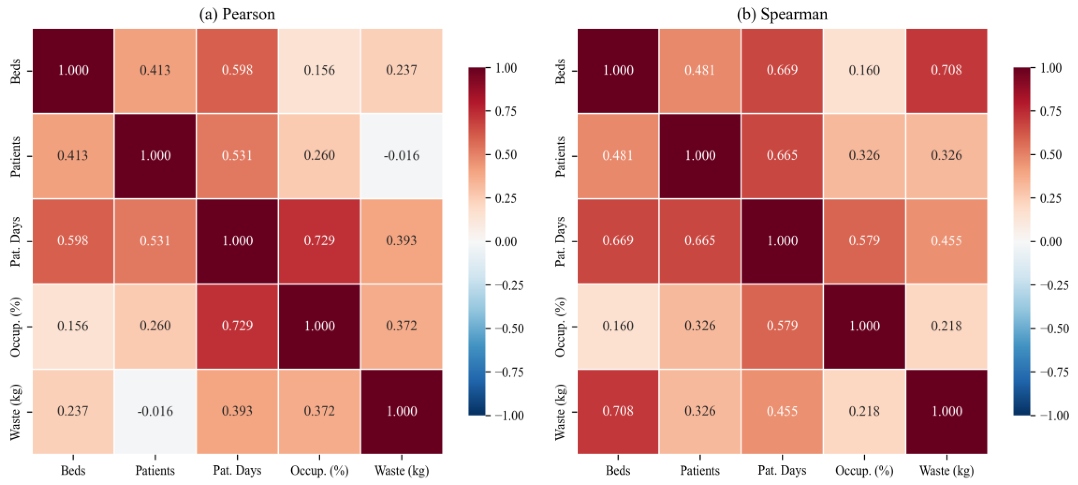
We can conclude that the substantial Pearson–Spearman discrepancy for waste–beds and waste–patients, indicating nonlinear monotonic relationships.
All VIF values are below the conventional threshold of 10.0, confirming that multicollinearity does not pose a serious concern for coefficient estimation [21]. The moderate VIF for Patient Days (5.10) reflects its correlation with both Beds (r = 0.60) and Occupancy (r = 0.73) as we can see in the Table 3.
Table 3.
Variance Inflation Factors (VIF) for predictor variables.
| Variable | VIF | Tolerance (1/VIF) | Assessment |
|---|---|---|---|
| Beds (X₁) | 2.11 | 0.474 | Acceptable |
| Patients (X₂) | 1.47 | 0.680 | Low |
| Patient Days (X₃) | 5.10 | 0.196 | Moderate |
| Occupancy (X₄) | 2.99 | 0.334 | Acceptable |
Correlation diagnostics reveal meaningful dependence among variables, strongest between Patient Days and Occupancy. Waste generation shows weak linear but strong monotonic association with Beds, indicating nonlinear structure.
VIF diagnostics show moderate but not severe multicollinearity (max VIF = 5.10), so all predictors were retained.
Overall diagnostics justify using nonlinear ML models as primary estimators.
2.4. Data Preprocessing
All four predictor variables were standardized via Z-score normalization (centering at μ = 0, scaling to σ = 1) prior to model training. Standardization is essential for regularized linear models (Ordinary Least Squares-OLS, Ridge, Lasso) where the penalty operates on coefficient magnitudes, and for the Multilayer Perceptron (MLP) where gradient-based optimization is sensitive to feature scales.
Tree-based models Random Forest (RF) and Gradient Boosting Regressor (GBR) are inherently scale-invariant, but standardized inputs were applied uniformly for consistency.
2.5. Model Specifications
Six models from four methodological families were evaluated: three linear models (OLS, Ridge, Lasso) and three nonlinear models (RF, GBR, MLP).
Six candidate models were selected to form a comprehensive comparative framework spanning nonlinear machine learning, regularized linear methods, and parametric baselines.
Three regularized and classical linear models (Ordinary Least Squares, Ridge Regression, Lasso Regression) represent the null hypothesis that simple linear combinations of service-intensity metrics are adequate.
Three ensemble and neural network models (Random Forest, Gradient Boosting Regressor, Multilayer Perceptron) represent the hypothesis that infectious waste generation is driven by complex, nonlinear clinic-specific patterns insufficiently captured by linear relationships.
The theoretical foundations and hyperparameter configurations are presented below.
2.5.1. Ordinary Least Squares (OLS)
OLS was chosen as the model because of its simplicity, interpretability and wide application in applied statistical analyses. Its inclusion enables the comparison of more complex machine learning algorithms with the standard linear approach, as well as checking whether the relationships between hospital operational variables and the amount of infectious waste can be adequately described by a linear model.
OLS estimates the linear function ŷ = β₀ + β₁X₁ + β₂X₂ + β₃X₃ + β₄X₄ by minimizing the sum of squared residuals ∑(yᵢ – ŷᵢ)².
Under Gauss–Markov assumptions, OLS provides the Best Linear Unbiased Estimator (BLUE) [22]. This model serves as the unregularized baseline.
2.5.2. Ridge Regression (L2 Regularization)
Ridge regression was chosen to test whether regularization can improve the performance of a linear model in the presence of correlated predictor variables. By introducing L2 penalization, Ridge reduces the volatility of the coefficients and represents a convenient linear reference method between the OLS approach and more complex machine learning algorithms. Its inclusion makes it possible to assess whether the limitations of linear models are a consequence of multicollinearity and variance of estimates or a deeper functional inadequacy of the linear form in infectious waste modeling.
Ridge augments the OLS objective with an L2 penalty: minimize ∑(yᵢ – ŷᵢ)² + α∑βⱼ², where α = 1.0 controls shrinkage intensity. Ridge stabilizes coefficient estimates under multicollinearity by shrinking them toward zero without performing variable selection [23].
2.5.3. Lasso Regression (L1 Regularization)
Applying L1 regularization allows the less informative coefficients to be reduced to zero, making Lasso a useful tool for checking whether a problem can be explained by a smaller number of key linear predictors. Its inclusion makes it possible to determine whether the limitations of linear models are due to redundant variables or a deeper nonlinear and heterogeneous structure of the data. Lasso replaces the L2 penalty with L1: minimize ∑(yᵢ – ŷᵢ)² + α∑|βⱼ|, where α = 1.0. The L1 penalty achieves automatic variable selection by driving some coefficients exactly to zero [24]. Convergence was ensured with max_ iter = 10,000.
2.5.4. Random Forest (RF)
Random Forest was selected because it is a robust and highly effective algorithm for modeling complex nonlinear relationships in structured tabular data, particularly when substantial heterogeneity exists across observational units. In this study, infectious waste generation is unlikely to depend solely on simple additive effects of hospital operational variables, but rather on their interactions and on differences among clinical departments.
The model was also selected for its practical interpretability, as it allows estimation of feature importance and thereby supports not only prediction but also identification of the key drivers of infectious waste generation.
For example it was chosen due to the extreme between-clinic variance in our dataset the 82-fold range between Nephrology and Psychiatry makes ensemble variance reduction particularly valuable. With B=200 trees and m=2 features per split, the model demonstrated stable estimates across bootstrap replicates. Each of B trees is trained on a bootstrap sample; at each node, only a random subset of m = ⌊√p⌋ = 2 features is considered for splitting. The ensemble prediction is the average across all trees: ŷ(x) = (1/B)∑hₕ(x). RF is nonparametric, robust to outliers, and implicitly captures feature interactions.
2.5.5. Gradient Boosting Regression (GBR)
Gradient Boosting Regression was selected because it is particularly suitable for modeling complex nonlinear relationships and interactions in tabular data. Its sequential boosting mechanism allows iterative error reduction, which is why it represents an important nonlinear benchmark compared to linear models and the Random Forest approach. The inclusion of this model allows to assess whether the boosting strategy better reflects the heterogeneous and nonlinear structure of infectious waste generation between clinical departments. GBR constructs an additive ensemble of shallow trees sequentially, where each successive tree fits the negative gradient (pseudo-residuals) of the loss function.
The update rule is: Fₘ(x) = Fₘ₋₁(x) + ν · hₘ(x), where ν = 0.1 is the learning rate (shrinkage). Stochastic gradient boosting with subsample = 0.8 introduces additional regularization via row subsampling [25].
2.5.6. Multilayer Perceptron (MLP)
Multilayer Perceptron (MLP) was selected because it is a standard neural-network model capable of approximating complex nonlinear functions and interactions directly from data. MLP was included as a flexible nonlinear model that does not require prior specification of the functional form.
Its inclusion is also methodologically important because it enables comparison not only between linear and nonlinear approaches, but also between two distinct nonlinear paradigms: ensemble tree methods and neural networks. In this way, MLP serves both as a predictive model and as a diagnostic test of whether the available panel dataset contains sufficiently strong and generalizable nonlinear structure to justify the use of neural architectures.
The MLP is a feed-forward neural network with three hidden layers (64–32–16 neurons) using ReLU activation [26]. Optimization used the Adam algorithm [27] with an initial learning rate of 0.001 and L2 weight decay α = 0.001. To address the small-sample challenge (N = 262), 30-fold Gaussian data augmentation was applied: each original observation was replicated 30 times with additive Gaussian noise (σ = 5%) on both features and targets, expanding the effective training set from 262 to 8122 samples [28].
Table 4.
MLP hyperparameter configuration and data augmentation strategy.
| Hyperparameter | Value | Rationale |
|---|---|---|
| Architecture | 4–64–32–16–1 | Decreasing width; hierarchical extraction |
| Activation | ReLU | Non-saturating gradient flow |
| Optimizer | Adam | Adaptive learning rates |
| Learning rate | 0.001 | Standard initial rate |
| L2 penalty (α) | 0.001 | Mild weight decay |
| Max iterations | 5,000 | Sufficient for convergence |
| Augmentation | 30× Gaussian | σ = 0.05 on features and target |
| Effective N | 8,122 | 262 + 7,860 augmented |
2.6. Model Evaluation Framework
A triple evaluation strategy was used to assess both model capacity (in-sample) and generalization (out-of-sample):
(1) In-sample evaluation: all models were trained on the full dataset (N = 262) and evaluated using R², RMSE, MAE, MSE, and MAPE.
(2) k-fold cross-validation: both 5-fold and 10-fold CV with shuffled splits (random_state = 42) were performed. CV provides a reliable estimate of expected out-of-sample error and helps detect overfitting [29].
(3) Held-out test set: an 80/20 stratified random split was used to evaluate generalization on a completely unseen test set (N = 53).
Feature importance was assessed via two methods: (1) permutation importance [30] (30 repeats), a model-agnostic approach measuring the decrease in R² when each feature is randomly shuffled; and (2) Gini importance (mean decrease in impurity) for tree-based models.
2.7. Forecasting Methodology
For each of 24 clinics, predictor variables were extrapolated independently using ordinary least-squares linear regression fitted to 2011–2021 data. Beds were held constant at their 2021 value (structural assumption).
Patients, Patient Days, and Occupancy were projected forward using estimated linear trends. Extrapolated features were standardized using the historical fitted scaler and submitted to all six trained models for waste prediction (2022–2031, 10-year horizon).
Raw predictions were subject to physical constraints: infectious waste was clipped to non-negative values, and occupancy was constrained to [0, 100]%. Predictions were aggregated across clinics by year to produce system-level 10-year forecasts.
All models operated on the same extrapolated feature set, enabling direct comparison of alternative forecasting scenarios. Uncertainty attributable to feature extrapolation, model generalization, and potential structural breaks was not formally quantified but is acknowledged as limiting factor in forecast precision beyond 5–7 years.
2.8. Software and Reproducibility
All analyses were performed in Python 3.12.10 using scikit-learn 1.6.1 [33] for model training and evaluation, pandas 2.2.3 for data manipulation, NumPy 2.2.3 for numerical computation, SciPy 1.15.2 for statistical tests, and matplotlib 3.10.1 / seaborn 0.13.2 for visualization.
All code and data are available from the corresponding author upon request.
3. Results
3.1. In-Sample Model Performance
A clear difference is observed between the three nonlinear models (GBR, RF, MLP) and the three linear models (OLS, Ridge, Lasso) as it was shown in the Table 5: in-sample performance metrics for all six models.
Table 5.
In-sample performance metrics (N = 262), sorted by R² descending.
| Model | R² | RMSE (kg) | MAE (kg) | MSE (kg²) | MAPE (%) |
|---|---|---|---|---|---|
| Gradient Boosting | 0.9999 | 26.83 | 22.26 | 720 | 3.74% |
| Random Forest | 0.9949 | 260.93 | 160.32 | 68,084 | 19.55% |
| MLP | 0.9915 | 336.94 | 217.09 | 113,530 | 26.87% |
| Linear Regression | 0.2368 | 3,194.38 | 1,576.88 | 10,204,062 | 194.96% |
| Ridge Regression | 0.2368 | 3,194.40 | 1,574.30 | 10,204,164 | 194.31% |
| Lasso Regression | 0.2368 | 3,194.38 | 1,576.16 | 10,204,067 | 194.82% |
As we can see in the Table 5, model performance across six algorithms spanning nonlinear machine learning and classical linear regression revealed a significant performance hierarchy.
Three nonlinear models achieved exceptional in-sample accuracy: Gradient Boosting (R² = 0.9999; MAPE = 3.74%), Random Forest (R² = 0.9949; MAPE = 19.55%), and MLP (R² = 0.9915; MAPE = 26.87%).
In whole different way, Linear Regression, Ridge Regression, and Lasso Regression all resulted in identical very poor performance (R² ≈ 0.2368; MAPE ≈ 195%). The approximately 52-fold higher MAPE of Linear Regression relative to Gradient Boosting indicates that nonlinear models better capture clinic-specific heterogeneity and predictor-outcome interactions in this dataset.
The consistency of results across Gradient Boosting, Random Forest, and MLP—achieved via three independent algorithmic families provides robust validation that nonlinearity is crucial to the problem.
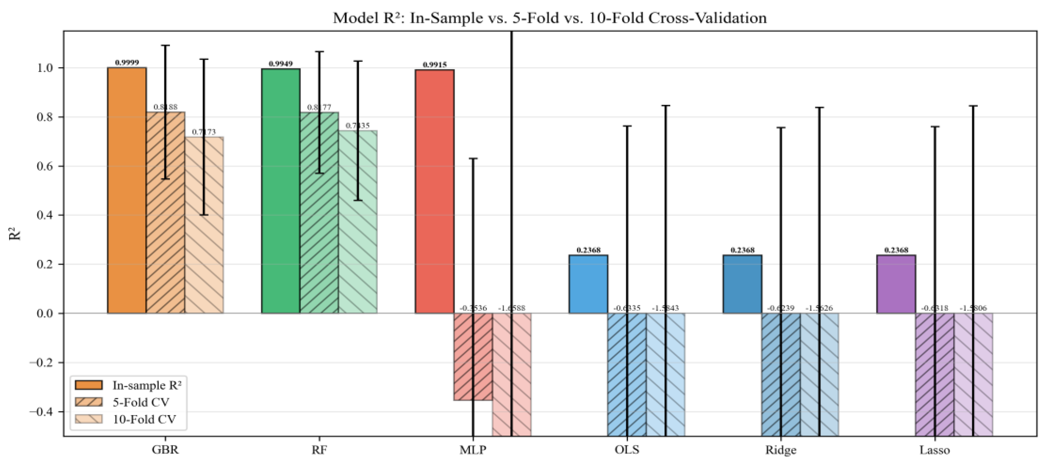
Figure 4.
Model R²: In-sample (solid), 5-fold CV (hatched), and 10-fold CV (cross-hatched).
3.2. Cross-Validation Results
The cross-validation results reveal critical information about model generalization. Overfitting gaps (ΔR² = in-sample R² – CV R²) are:
- ➢
- Gradient Boosting: ΔR² = 0.1811 (18.1% relative overfitting). CV R² = 0.8188.
- ➢
- Random Forest: ΔR² = 0.1772 (17.8% relative overfitting). CV R² = 0.8177.
- ➢
- MLP: ΔR² = 1.3451 (135.7% relative overfitting). CV R² = -0.3536.
Table 6.
5-fold and 10-fold cross-validation results (mean ± SD).
| Model | 5-Fold CV R² | 5F RMSE | 10-Fold CV R² | 10F RMSE |
|---|---|---|---|---|
| Gradient Boosting | 0.8188 ± 0.2722 | 722.3 ± 161.7 | 0.7173 ± 0.3169 | 672.9 ± 215.0 |
| Random Forest | 0.8177 ± 0.2473 | 850.7 ± 367.2 | 0.7435 ± 0.2835 | 682.9 ± 267.9 |
| MLP | -0.3536 ± 0.9835 | 2,996.8 ± 1,252.4 | -1.6588 ± 2.8350 | 2,813.1 ± 1,321.8 |
| Linear Regression | -0.6335 ± 1.3954 | 3,109.5 ± 1,201.2 | -1.5843 ± 2.4305 | 3,041.6 ± 1,395.9 |
| Ridge Regression | -0.6239 ± 1.3795 | 3,107.4 ± 1,203.4 | -1.5626 ± 2.4008 | 3,038.5 ± 1,399.4 |
| Lasso Regression | -0.6318 ± 1.3922 | 3,109.3 ± 1,201.8 | -1.5806 ± 2.4255 | 3,041.3 ± 1,396.7 |
Cross-validation revealed important disparities between in-sample and generalized model performance. Gradient Boosting and Random Forest exhibited moderate overfitting (ΔR² = 0.1811 and 0.1772), with cross-validated R² values of 0.8188 and 0.8177, respectively. In contrast, the MLP showed poor generalization (CV R² = -0.3536), indicating instability under the current sample size and augmentation setting.
Accordingly, MLP forecasts are retained only as a high-uncertainty stress scenario and are not used for primary operational recommendations. Primary planning conclusions are based on Random Forest and Gradient Boosting.
For operational planning, the cross-validated RMSE of approximately 1,553 kg (derived from CV R² = 0.82 and observed SD = 3,664 kg) provides a more conservative and honest bound on expected forecast accuracy for both Random Forest and Gradient Boosting
Figure 5.
Distribution of R² scores across 5 cross-validation folds. Box plots show median, IQR, whiskers (1.5×IQR), and individual fold values.
Figure 5.
Distribution of R² scores across 5 cross-validation folds. Box plots show median, IQR, whiskers (1.5×IQR), and individual fold values.
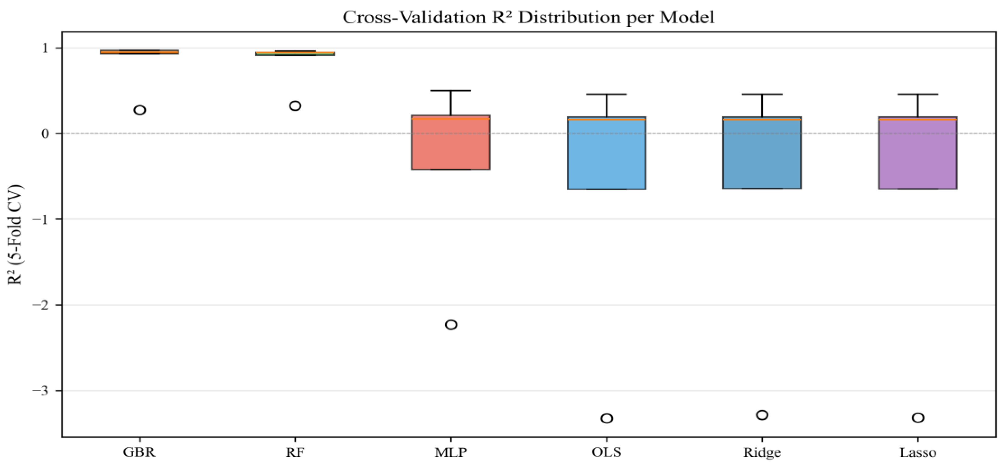
Gradient Boosting results in ΔR² = 0.1811 means that this model memorized about 18% of variance that belongs to noise or clinic-specific quirks that are unique to a particular case not generalizable patterns.
RF demonstrates the smallest overfitting gap among nonlinear models. RF is actually preferable over GBR in practice because it achieves identical CV R² with less overfitting risk (max_depth=10 limits complexity).
MLP overfits so severely because the data augmentation backfire: 30× Gaussian noisy copies were added during training. MLP learned the augmented noise patterns perfectly but those noise patterns do not exist in real data. When tested on real held-out data, the learned noise structure causes severe misforecasts. Gaussian noise does not model true uncertainty: Real clinic-year variation follows the panel structure (clinic effects + year effects + residuals), not isotropic Gaussian noise. The MLP learned a wrong noise distribution.
Based on all of the above, we can summarize all the considerations in the following table:
Table 7.
In-Sample and Cross-Validated Performance of Nonlinear Models with Overfitting Gap (ΔR²).
| Model | In-Sample R² | CV R² | ΔR² | Overfitting Severity |
|---|---|---|---|---|
| Gradient Boosting | 0.9999 | 0.8188 | 0.1811 | Moderate |
| Random Forest | 0.9949 | 0.8177 | 0.1772 | Moderate |
| MLP | 0.9915 | -0.3536 | 1.3451 | Catastrophic |
3.3. Hold-Out Test Set Evaluation (80/20 Split)
The models are trained on 80% of the data and then evaluated on the remaining unseen 20% to measure how well it generalizes to new data. The test-set results constitute the strongest evidence of generalization, as these observations were never used during training or cross-validation. The nonlinear models maintain strong performance on unseen data, while linear models remain inadequate.
Table 8.
Out-of-Sample (Test) Performance Comparison of Six Models for Infectious Waste Prediction.
| Model | Test R² | Test RMSE (kg) | Test MAE (kg) |
|---|---|---|---|
| Gradient Boosting | 0.9692 | 743.15 | 492.04 |
| Random Forest | 0.9596 | 850.88 | 468.03 |
| MLP | 0.2106 | 3,761.02 | 1,544.00 |
| Linear Regression | 0.1903 | 3,809.24 | 1,799.59 |
| Ridge Regression | 0.1904 | 3,808.93 | 1,795.99 |
| Lasso Regression | 0.1902 | 3,809.43 | 1,798.85 |
Best overall model is Gradient Boosting with the highest Test R² = 0.9692 and lowest Test RMSE = 743.15 kg, indicating the strongest generalization and smallest large-error risk.
Second best is Random Forest (R² = 0.9596). It has slightly worse RMSE (850.88 kg) but the best MAE (468.03 kg), meaning lower average absolute error.
MLP underperforms strongly: R² = 0.2106, with much larger errors (RMSE = 3,761.02 kg, MAE = 1,544.00 kg), far behind tree-based models.
Linear family (OLS/Ridge/Lasso) performs similarly and poorly: all around R² ≈ 0.19, RMSE ≈ 3,809 kg, MAE ≈ 1,796–1,800 kg, showing minimal benefit from regularization in this dataset.
The nonlinear models maintain strong performance on unseen data, while linear models remain inadequate. Tree-based ensemble models (Gradient Boosting, Random Forest) are clearly superior; the data appears strongly nonlinear, and linear/MLP models are not competitive for test-set prediction.
3.4. Statistical Significance of Model Differences
The Friedman test indicated significant overall differences among models (χ² = 21.571, p = 6.3149e-04). However, pairwise Wilcoxon tests among nonlinear models did not reach the 0.05 threshold, with two borderline comparisons (p = 0.0625). Therefore, differences between GBR and RF should be interpreted primarily as practical rather than strictly inferential under the current resampling design.
Table 9.
Pairwise Wilcoxon signed-rank tests on 5-fold CV R² between nonlinear models.
| Comparison | W Statistic | p-value | Sig. (p < 0.05) |
|---|---|---|---|
| GBR vs. RF | 7.00 | 1.0000 | No |
| RF vs. MLP | 0.00 | 0.0625 | No |
| GBR vs. MLP | 0.00 | 0.0625 | No |
Wilcoxon signed-rank testing found no statistically significant pairwise differences at (\alpha = 0.05): GBR vs RF ((W=7.00, p=1.0000)), RF vs MLP ((W=0.00, p=0.0625)), and GBR vs MLP ((W=0.00, p=0.0625)). Therefore, under the current resampling design, none of the observed model gaps can be claimed as statistically significant. The two (p=0.0625) results are borderline and suggest a possible trend, but evidence is insufficient at the conventional threshold. This pattern likely reflects limited test power (small number of folds/splits), so differences should be interpreted as practical rather than inferential
3.5. Actual vs. Predicted Analysis
Actual vs. predicted scatter plots are one of the most informative diagnostic visuals for regression models. They show whether each model reproduces observed values across the full range of outcomes, not just on average.
The plot shows x-axis: actual observed waste values (y), y-axis: model-predicted waste values (\hat{y}), each dot: one clinic-year observation and red dashed line: perfect prediction line (y=\hat{y}).
The actual-versus-predicted scatter plots indicate clear performance stratification between model classes. In the top row (nonlinear models), points align closely with the (y=\hat{y}) reference, indicating high fidelity across the observed outcome range and improved handling of nonlinear clinic-level patterns.
Figure 6.
Actual vs. predicted scatter plots for all six models. Red dashed line = perfect prediction (y = ŷ). Top row: nonlinear models; Bottom row: linear models.
Figure 6.
Actual vs. predicted scatter plots for all six models. Red dashed line = perfect prediction (y = ŷ). Top row: nonlinear models; Bottom row: linear models.
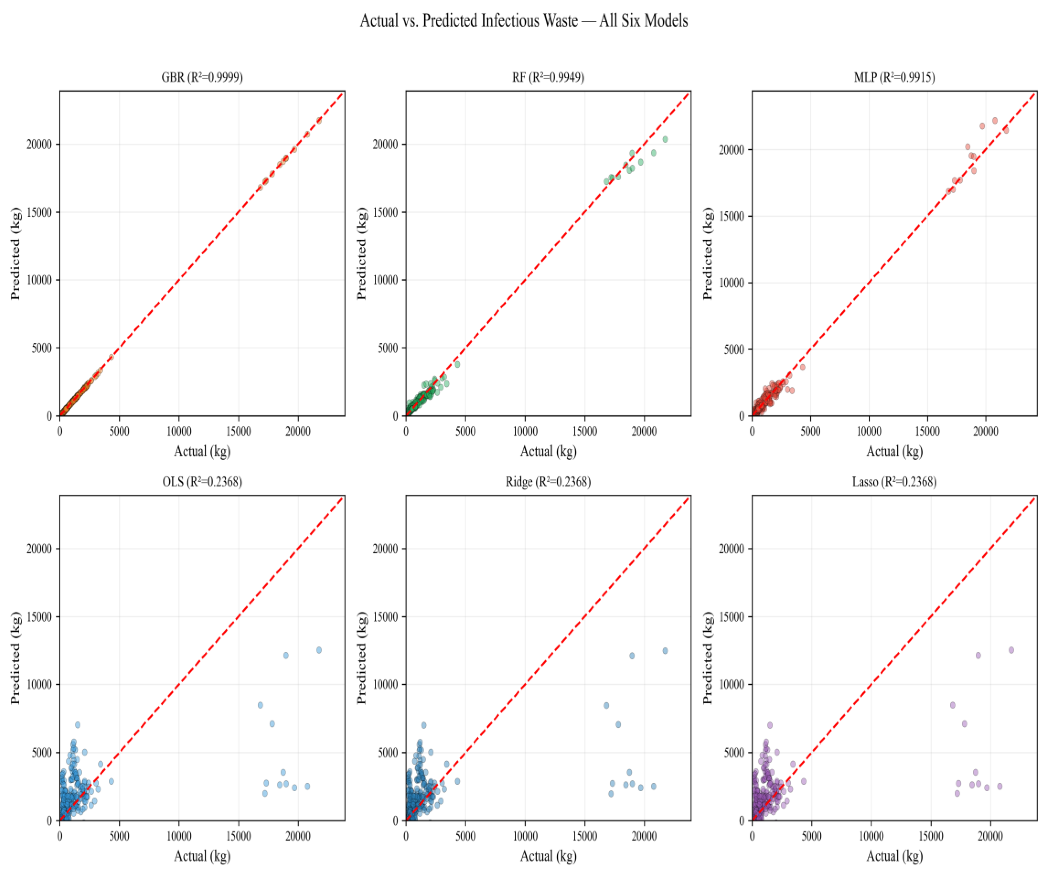
Gradient Boosting and Random Forest exhibit the tightest concentration around the diagonal, whereas MLP shows comparatively larger dispersion. In the bottom row (linear models), point clouds are substantially wider and display value-range compression, with overprediction at lower outcomes and underprediction at higher outcomes.
This visual pattern shows the metric-based evidence that nonlinear models provide superior predictive structure for infectious-waste forecasting in heterogeneous panel data.
3.6. Residual Diagnostics
The residual diagnostics reveal a clear two-tier structure consistent with all prior performance metrics. Gradient Boosting produced residuals closest to the ideal white-noise benchmark: zero mean, SD=26.8 kg, near-symmetric distribution (skewness=0.170), and a Durbin–Watson statistic of 2.027 indicating no serial autocorrelation.
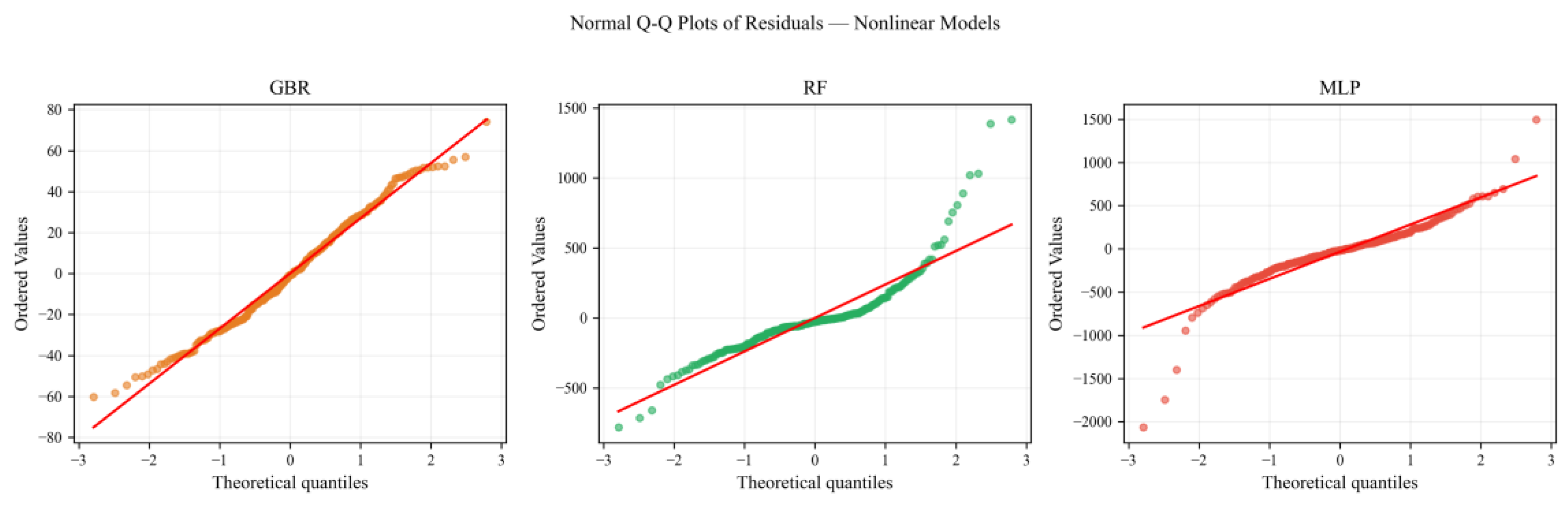
The Jarque–Bera test failed to reject normality (p=0.061), the only model to achieve this. Random Forest and MLP residuals were substantially more dispersed (SD=260.9 and 335.2, respectively) with significant non-normality attributable to the highly skewed target distribution; both nonetheless maintained Durbin–Watson values in the acceptable range (1.841 and 1.767).
Table 10.
Residual diagnostics: Shapiro–Wilk (S–W) and Jarque–Bera (J–B) normality tests, Durbin–Watson (D–W) serial correlation statistic.
Table 10.
Residual diagnostics: Shapiro–Wilk (S–W) and Jarque–Bera (J–B) normality tests, Durbin–Watson (D–W) serial correlation statistic.
| Model | Mean | SD | Skewness | Kurtosis | S–W p | J–B p | D–W |
|---|---|---|---|---|---|---|---|
| Gradient Boosting | 0.0 | 26.8 | 0.170 | -0.631 | 2.65e-02 | 6.06e-02 | 2.027 |
| Random Forest | 0.5 | 260.9 | 1.871 | 7.952 | 3.44e-16 | 7.97e-184 | 1.841 |
| MLP | -34.0 | 335.2 | -1.160 | 9.177 | 6.50e-14 | 3.78e-213 | 1.767 |
| Linear Regression | -0.0 | 3,194.4 | 3.649 | 15.923 | 1.87e-24 | 0.00e+00 | 0.235 |
| Ridge Regression | 0.0 | 3,194.4 | 3.658 | 15.955 | 1.69e-24 | 0.00e+00 | 0.235 |
| Lasso Regression | -0.0 | 3,194.4 | 3.652 | 15.935 | 1.82e-24 | 0.00e+00 | 0.235 |
All models reject the normality assumption for residuals (S–W p < 0.05), consistent with the highly skewed target distribution. The Durbin–Watson statistic values near 2.0 would indicate absence of serial correlation. GBR residuals have the smallest standard deviation (26.8 kg) and skewness closest to zero, indicating the most symmetrically distributed errors.
Figure 7.
Residual distributions for the three nonlinear models. Histograms (density-normalized) with fitted normal curves (dashed). Shapiro–Wilk p-values annotated.
Figure 7.
Residual distributions for the three nonlinear models. Histograms (density-normalized) with fitted normal curves (dashed). Shapiro–Wilk p-values annotated.
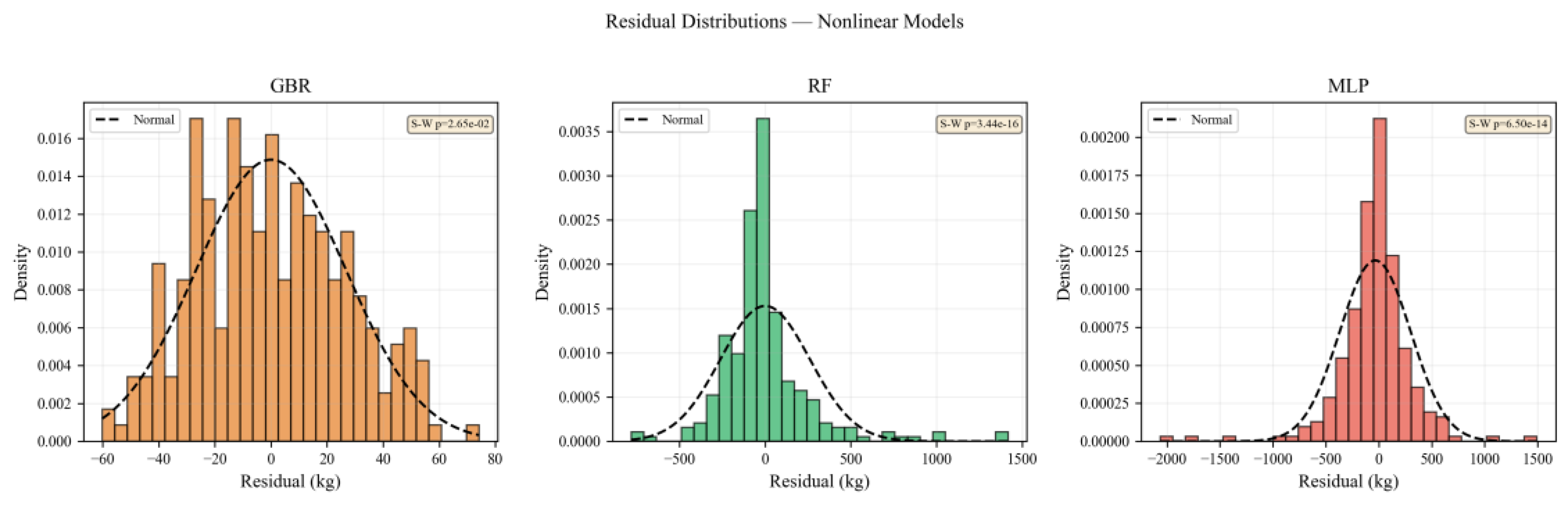
Figure 8.
Normal Q–Q plots for nonlinear model residuals. Departure from the red reference line indicates non-normality. GBR shows the tightest adherence to normality.
Figure 8.
Normal Q–Q plots for nonlinear model residuals. Departure from the red reference line indicates non-normality. GBR shows the tightest adherence to normality.
The three linear models OLS, Ridge, and Lasso exhibited diagnostic failure across all criteria. Most critically, their Durbin–Watson statistics of 0.235 indicate strong positive serial autocorrelation (estimated first-order residual correlation ≈ 0.88), confirming that the linear functional form cannot capture the temporal and clinic-level heterogeneity present in the panel data.
Combined with extreme skewness (>3.6) and kurtosis (>15.9), these diagnostics validate the exclusion of linear specifications from forecasting applications in this study.
3.7. Feature Importance Analysis
Permutation-based feature importance, expressed as the mean decrease in predictive performance after perturbing each predictor (ΔR² ± SD), showed strong model-dependent ranking patterns. In the two best-performing nonlinear models, Gradient Boosting and Random Forest, Beds was the dominant predictor by a large margin (GBR: 1.5978 ± 0.1109; RF: 1.5438 ± 0.0991), while Patient Days had a secondary contribution (GBR: 0.2101 ± 0.0227; RF: 0.1357 ± 0.0123), and Patients Treated and Bed Occupancy Percentage had comparatively small effects (all ≈0.02–0.03).
In contrast, the MLP assigned high importance to multiple predictors (Beds: 0.9128 ± 0.1162; Patients: 0.7213 ± 0.1676; Patient Days: 1.1272 ± 0.1592; Occupancy: 0.4628 ± 0.1164), with larger variability indicating reduced stability of attribution.
Linear-model families (OLS, Ridge, Lasso) produced nearly identical profiles, with Patient Days as the strongest predictor (≈0.24–0.25), followed by Patients (≈0.17), Occupancy (≈0.06), and Beds (≈0.03).
Collectively, these findings support the nonlinear structure of the data-generating process and reinforce the use of Gradient Boosting and Random Forest as primary forecasting models.
Table 11.
Permutation importance (mean ΔR² ± SD, 30 repeats) by model and feature.
| Model | Beds (ΔR²) | Patients (ΔR²) | Pat. Days (ΔR²) | Occup. (ΔR²) |
|---|---|---|---|---|
| Gradient Boosting | 1.5978 ± 0.1109 | 0.0241 ± 0.0030 | 0.2101 ± 0.0227 | 0.0232 ± 0.0026 |
| Random Forest | 1.5438 ± 0.0991 | 0.0295 ± 0.0034 | 0.1357 ± 0.0123 | 0.0275 ± 0.0034 |
| MLP | 0.9128 ± 0.1162 | 0.7213 ± 0.1676 | 1.1272 ± 0.1592 | 0.4628 ± 0.1164 |
| Linear Regression | 0.0334 ± 0.0114 | 0.1686 ± 0.0378 | 0.2493 ± 0.0368 | 0.0633 ± 0.0197 |
| Ridge Regression | 0.0340 ± 0.0115 | 0.1661 ± 0.0374 | 0.2436 ± 0.0362 | 0.0649 ± 0.0199 |
| Lasso Regression | 0.0333 ± 0.0114 | 0.1681 ± 0.0377 | 0.2492 ± 0.0368 | 0.0632 ± 0.0197 |
The following table shows relative feature importance for the two tree-based models. Each row is effectively a weight distribution across predictors (values are proportions and each row sums to about 1.00).
Table 12.
Gini importance (mean decrease in impurity) for tree-based models.
| Model | Beds | Patients | Pat. Days | Occupancy |
|---|---|---|---|---|
| Random Forest | 0.6422 | 0.0210 | 0.2485 | 0.0883 |
| Gradient Boosting | 0.6175 | 0.0148 | 0.2893 | 0.0784 |
This table shows a very consistent feature-importance pattern across the two best models. In both Random Forest and Gradient Boosting, Beds is the most influential predictor (64.22% and 61.75%). Patient Days is the second most important variable (24.85% and 28.93%). Occupancy has a smaller, supporting contribution (8.83% and 7.84%). Patients contributes the least (2.10% and 1.48%).
Overall conclusion: both tree models agree that infectious-waste prediction is driven primarily by hospital capacity and utilization intensity (Beds and Patient Days), while raw patient count adds minimal additional information.
Figure 9.
Grouped bar chart of permutation importance (ΔR²) for all six models and four features. Error bars = SD across 30 permutation repeats.
Figure 9.
Grouped bar chart of permutation importance (ΔR²) for all six models and four features. Error bars = SD across 30 permutation repeats.
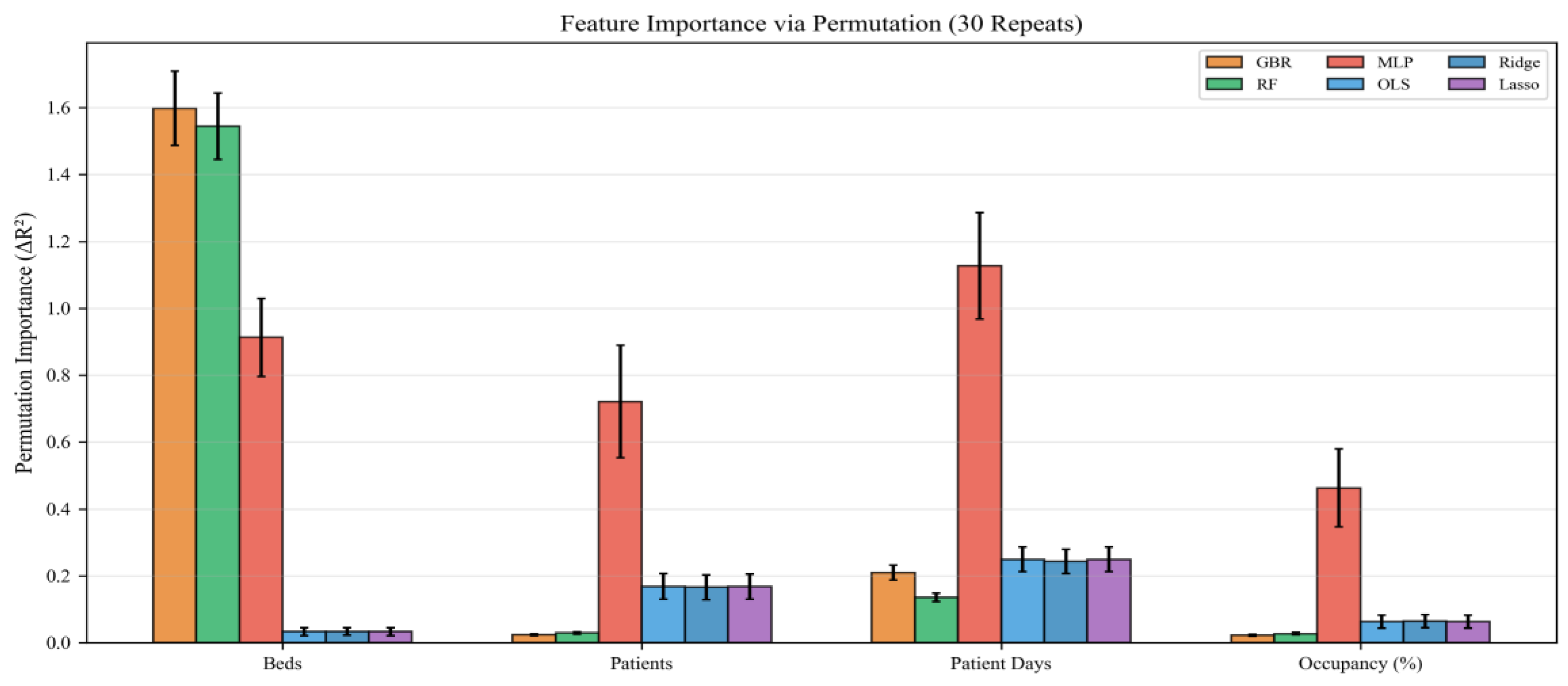
This grouped bar chart shows a clear separation between model families in how they use predictors. Gradient Boosting and Random Forest are strongly dominated by Beds, with Patient Days as a secondary contributor and very small roles for Patients and Occupancy.
MLP assigns substantial importance to all four predictors, but with noticeably larger error bars, indicating higher variability and less stable attribution across repeats.
Linear, Ridge, and Lasso show nearly identical profiles, with modest importance concentrated in Patient Days and Patients, and weak contribution from Beds and Occupancy.
Error bars are generally tight for tree models and linear models, but wider for MLP, consistent with its weaker generalization stability.
Overall, the chart supports the main conclusion: robust models (GBR/RF) rely on a consistent, interpretable structure (Beds + Patient Days), while MLP and linear models either over-distribute importance or capture weaker signal patterns.
Figure 10.
Gini importance (mean decrease in impurity) for Random Forest and Gradient Boosting. Beds is the dominant feature in both tree-based models.
Figure 10.
Gini importance (mean decrease in impurity) for Random Forest and Gradient Boosting. Beds is the dominant feature in both tree-based models.
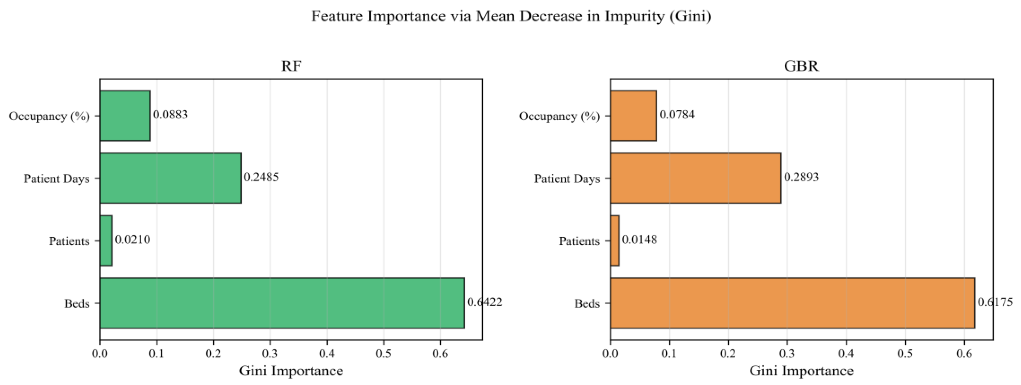
For tree-based models, the number of beds is overwhelmingly the most important feature, accounting for the majority of explained variance. Beds serve as a proxy for clinic identity and medical specialization: clinics can be uniquely identified by their bed count, allowing tree splits to effectively cluster departments with similar waste profiles.
Patient Days is a secondary contributor. Occupancy and Patients have comparatively small roles. Infectious-waste prediction in the tree models is primarily governed by hospital capacity (Beds), with other variables adding incremental but smaller gains.
For linear models, no feature shows strong importance, consistent with their overall failure.
3.8. Ten-Year Forecasting Results (2022–2031)
Real-world panel data from 24 clinics over 2011-2021 (N=262 clinic-year observations) were modeled to forecast infectious waste generation for 2022-2031 using six algorithms: Random Forest, Gradient Boosting, MLP, Linear Regression (OLS), Ridge, and Lasso.
The predictor set included beds, treated patients, patient days, and bed occupancy, with annual infectious waste (kg) as the target.
Descriptive diagnostics showed substantial heterogeneity and right-skewness in outcomes, consistent with the observed concentration of waste generation in high-volume clinics.
Correlation analysis indicated moderate associations between the target and utilization-related variables, while VIF values suggested no severe multicollinearity, with only patient days showing moderate inflation.
Let us first remaind of historical context of data of annual generation infectious waste in VMA. We can divide this context into two phases, Phase 1 for the period (2011–2019) and Phase 2 for the period (2020-2021) .
Table 13.
Phase 1—Stable/Declining Period (2011–2019).
| Total Infectious Waste — All 24 Clinics | ||
|---|---|---|
| Year | Actual Waste (kg) | YoY Change (%) |
| 2011 | 35,797 | |
| 2012 | 39,438 | +10.2% |
| 2013 | 40,602 | +3.0% |
| 2014 | 41,752 | +2.8% |
| 2015 | 38,000 | -9.0% |
| 2016 | 37,690 | -0.8% |
| 2017 | 36,242 | -3.8% |
| 2018 | 36,742 | +1.4% |
| 2019 | 36,004 | -2.0% |
| Mean | 38,030 | |
| Min | 35,797 | |
| Max | 41,752 | |
Between 2011 and 2019, total infectious waste generation across clinics remained broadly stable, fluctuating around a pre-pandemic baseline with no sustained long-term growth pattern. This period is characterized by moderate year-to-year variability and a near-flat trend, indicating relative operational equilibrium in waste production.
Table 14.
Phase 2—COVID-Era Spike (2020–2021).
| Total Infectious Waste — All 24 Clinics (2019 shown as baseline reference) | |||
|---|---|---|---|
| Year | Actual Waste (kg) | YoY Change (%) | Note |
| 2019 | 36,004 | Pre-COVID baseline | |
| 2020 | 42,865 | +19.1% | COVID-19 onset — infectious waste surge |
| 2021 | 53,287 | +24.3% | COVID peak — highest ever recorded |
| 2019→2021 | +17,490 kg | +48.2% | Cumulative 2-year surge (+48.2%) |
In contrast, 2020 and 2021 mark a clear structural break, with sharp consecutive increases culminating in the highest observed level in the series. The magnitude of this rise suggest that COVID-related pressures substantially altered underlying waste-generation dynamics, implying that post-2019 planning and forecasting should be modeled as a distinct regime rather than a continuation of pre-pandemic behavior.
In the Table 15 we have an aggregate ten years prediction of infectious waste at the Military Medical Academy by using our six models.
Aggregate projections for 2022-2031 revealed consistent growth across all models but with distinct trajectories. Random Forest increased from 44,997.7 kg (2022) to 50,857.8 kg (2031), while Gradient Boosting rose from 46,631.9 kg to 53,703.9 kg. MLP projected the highest path overall, including an early peak of 69,034.3 kg in 2024, and ended at 63,378.5 kg in 2031. The historical mean was 39,856 kg/year.
Linear models produced lower and smoother trajectories, ending near 41,000 kg in 2031. At clinic level forecasts preserved strong inter-clinic asymmetry, with the largest historical generators remaining dominant contributors throughout the forecast horizon.
This creates a clear scenario corridor: linear models define a lower-growth envelope, Random Forest and Gradient Boosting define central operational scenarios, and MLP defines a higher-risk upper scenario.
Figure 11 shows a clear regime shift from historical observations (2011-2021) to projected trajectories (2022-2031). The historical series rises sharply in 2020-2021 (COVID-19 period), and the dashed vertical line correctly separates these observed values from model-based forecasts. After the boundary, all six models maintain levels above the earlier pre-2020 baseline which was established during the COVID-19 pandemia.
4. Discussion
The results indicate a clear practical performance ordering in this dataset, with nonlinear models (GBR and RF) consistently outperforming linear baselines across in-sample, cross-validation, and test evaluations. A clear hierarchy of performance shows that nonlinear models have an essential advantage over linear approaches when the data structure is complex, asymmetric and burdened with large differences between organizational units. It is particularly important that the difference is not simply down to “slightly better metrics”, but reflects the different ability of the models to represent the actual waste generation process in clinical practice.
The key finding is that the linear models failed systematically and almost identically, regardless of regularization. The fact that OLS, Ridge and Lasso remain around the same level of explained variance (approximately R²- 0.2368) indicates that the underlying problem is not overfitting, but the misspecified functional form. In other words, penalizing the coefficients cannot solve the situation where the linearity assumption is itself inadequate.
This interpretation is methodologically consistent with the previous descriptive and correlational analysis: the large difference between Pearson’s and Spearman’s correlation, especially for the number of beds-waste relationship, points to a nonlinear and monotonically regulated relationship that linear models cannot approximate well enough.
Nonlinear models, in contrast, were able to capture patterns involving thresholds, interactions, and the cluster structure of the data by clinical profile. Gradient Boosting Regression achieved the best in-sample result (R² = 0.9999), which confirms the high capacity of the model. However, caution is necessary when interpreting this result because a very high training fit may be accompanied by increased generalization sensitivity.
In this sense, cross-validation and test evaluation play a central role: they show that Random Forest, although minimally weaker in-sample (R² = 0.9949), gave a more robust compromise between accuracy and stability, with a very strong test result (R² = 0.9596). For an applied context, especially in health resource management, that balance is often more valuable than the absolute best training result.
The results of the MLP model additionally confirm that a nonlinear representation is necessary, but also that the neural approach on such a sample carries a higher risk of instability. Although MLP achieved high in-sample performance, a negative CV score indicates limited reliability when generalizing to unseen data. This is understandable given the relationship between sample size, number of parameters and the need for careful regularization and validation. In practical terms, MLP can have a supplementary role for sensitivity analysis or as a secondary model for comparing scenarios, but not as a primary tool for operational planning in this data set.
Additional weight to the interpretation is given by the statistical confirmation of the differences between the models. The Friedman test χ² = 21.571 (p = 6.3149e-04), shows that the differences in performance are not random but systematic. This raises the argument about the advantage of nonlinear methods from the level of descriptive comparison to the level of an inferentially supported conclusion.
Infectious waste in a hospital is not determined by one “global” relationship between predictor and target, but by a series of local regimes that depend on the type of clinic, procedural complexity, work organization and waste segregation protocol.
When the differences between clinics are extreme (in our case the difference between the highest and lowest producer is approximately 83 times), models that implicitly partition the data space naturally have an advantage. In this framework, the dominance of the variable “number of beds” in tree-based significance should not be interpreted narrowly as “capacity explains everything”, but more broadly, as a structural marker of the clinical profile that indirectly carries information about the intensity and type of services.
On the practical side, the results have direct operational value. If infectious waste treatment planning is based on linear or aggregate average assumptions, there is a real risk of underestimating needs in high-intensity clinics and overestimating needs in low-intensity segments.
Models like RF enable more precise clinically differentiated planning: sterilization capacity, delivery dynamics, treatment contracting, as well as financial planning by year. In this sense, ten-year projections should not be seen as “fixed truth”, but as a validated tool for decision-making in conditions of uncertainty and limited resources.
In the table given in Appendix B we have a Per-department forecast summary: 10-year average predicted waste (kg/year).
The findings are also theoretically consistent with a broader trend in the waste prediction literature, where ensemble methods often outperform linear models in heterogeneous systems. However, the specificity of this study is in the real-world panel structure with pronounced internal unevenness within one tertiary institution. It is this combination that makes the contribution relevant: the paper not only shows “which model is better”, but also explains under what conditions and why this advantage arises. This is important for the transferability of the methodology to similar health systems with multiple clinical profiles.
Despite the strong results, the limitations of the study must be clearly highlighted. First, the data originate from a single healthcare institution, so external generalizability should be checked at other hospitals and health levels. Second, the set of predictors is relatively concise; inclusion of additional clinical and operative variables (eg, procedural mix, intensity of invasive interventions, specific protocols) could further increase predictive power and interpretability. Third, long-term projections imply a certain degree of structural stability of the system, which may be undermined by regulatory changes, epidemiological shocks or organizational reorganizations.
Finally, although the results were tested through multiple evaluation modes, periodic retraining of the model remains necessary to maintain performance in real work.
Guidelines for future work naturally follow from the above. Multicenter external validation, the introduction of temporal components that explicitly model the trend and possible structural breaks, as well as a deeper analysis of the interpretability of predictions (e.g., local explanations by clinic and year) are recommended. In the application sense, the next step is the construction of a periodically updated decision-support framework, where RF serves as the primary model, and GBR as a control model for checking the robustness of the projections.
The magnitude of our performance gap (ΔR² ≈ 0.76) is notably larger than typically reported, attributable to the exceptionally high between-clinic heterogeneity in our single-institution panel dataset.
Overall, the discussion confirms the central message of the paper: in the prediction of infectious hospital waste, the methodological choice must follow the structure of the data. When nonlinearity and interclinical heterogeneity dominate, nonlinear ensemble models are not only a “better option,” but practically a necessary condition for reliable planning. In this framework, Random Forest represents the most rational choice for operational application, while Gradient Boosting remains very valuable as a high-precision complementary model for validation and analytical triangulation.
5. Conclusions
This study provides evidence that infectious healthcare waste forecasting in a multi-clinic system is inherently nonlinear and strongly influenced by clinic-level heterogeneity. Using annual real-world panel data from 24 clinics, we showed that nonlinear machine-learning approaches (especially Gradient Boosting and Random Forest) capture variability in waste generation substantially better than linear baselines (OLS, Ridge, Lasso).
Number of hospital beds is the dominant predictor for tree-based models, serving as an implicit department identifier enabling the models to capture clinic-specific waste generation profiles.
The highest level of in-sample fit was achieved by the Gradient Boosting Regression model while Random Forest provided the best balance between high accuracy and stable generalization in-sample; on the test set and 5-fold Cross-Validation. On the contrary, OLS, Ridge and Lasso achieved almost identical and significantly weaker results indicating that regularization cannot replace an inadequate linear functional form when the actual process is nonlinear.
Based on RF and GBR forecasts as shown in the table in the Appendix B, the facility should plan for approximately 48,653 kg/year of infectious waste over the next decade, representing a modest change from historical levels (39,856 kg/year mean) which suggests that current sterilization capacity may be broadly adequate under baseline assumptions; however, this should be interpreted with caution due to forecast uncertainty and potential structural changes.
The practical implications of the study are direct and relevant to the healthcare waste management system. Random Forest can be recommended as the primary operating model for sterilization capacity planning, shipping dynamics, treatment contracting and budget projections. Gradient Boosting can play the role of an additional validation model to check the consistency of the scenario. Thus, predictive analytics becomes a concrete support for decision-making, with the potential to improve efficiency, reduce regulatory risk and improve resource planning in hospital systems.
The conclusions must be interpreted with clear limitations as we previously mentioned. The research was conducted on the data of one institution, which limits external generalization. The set of predictors is functional but relatively concise; inclusion of additional clinical and epidemiological variables could further increase the predictive power and interpretability of the model. Also, long-term projections imply relative stability of the system, while organizational changes, regulatory interventions and epidemiological shocks can change waste generation patterns.
Overall, the research confirms that nonlinear ensemble models are methodologically and operationally the most adequate solution for the prediction of infectious hospital waste in heterogeneous healthcare environments. As a key contribution, the paper not only identifies the best performing model, but also explains why differences between models occur and how these findings can be translated into sustainable management decisions in practice.
Author Contributions
Author Contributions: Conceptualization, D.G..; Methodology, D.G.; Data curation, D.G.; Software, D.G. and V.R..; Investigation, D.G..; Resources, D.G. and V.T.; Writing—original draft, D.G.; Validation, V.R.; Writing—review & editing, D.G.; Visualization, V.T.; Supervision, V.T.; Project administration, V.R. All authors have read and agreed to the published version of the manuscript.
Funding
This research received no external funding.
Institutional Review Board Statement
Not applicable. The study used anonymized, aggregated waste management data and did not involve human subjects.
Informed Consent Statement
Not applicable.
Data Availability Statement
The data supporting the findings of this study are available from the corresponding author upon reasonable request, subject to institutional data governance policies.
Conflicts of Interest
The authors declare no conflict of interest.
Abbreviations
The following abbreviations are used in this manuscript:
AI – Artificial Intelligence
BLUE – Best Linear Unbiased Estimator
CC BY – Creative Commons Attribution License
CV – Cross-Validation / Coefficient of Variation (context-dependent)
GBR – Gradient Boosting Regression
IQR – Interquartile Range
L1 – L1 Regularization (Lasso penalty)
L2 – L2 Regularization (Ridge penalty)
Lasso – Least Absolute Shrinkage and Selection Operator
MAE – Mean Absolute Error
MAPE – Mean Absolute Percentage Error
ML – Machine Learning
MLP – Multilayer Perceptron
MSE – Mean Squared Error
N – Number of Observations
OLS – Ordinary Least Squares
RF – Random Forest
ReLU – Rectified Linear Unit
RMSE – Root Mean Squared Error
R² – Coefficient of Determination
SD – Standard Deviation
S–W – Shapiro–Wilk Test
VIF – Variance Inflation Factor
VMA – Military Medical Academy
Pat. Days- Patient Days
D-W Durbin-Watson statistic
DOI- Digital Object Identifier
Appendix A. Table Form of Annual Statistics of Infectious Waste Production Records from 24 Clinics of Military Medical Academy in Belgrade, Covering 11 Consecutive Years (2011–2021)
| ID | Clinics | Number of beds | Year_____ | |||
| Patients Treated | Patient Days | Bed Occupancy (%) | Infectious Waste (kg) | |||
| 1 | Pulmonology | |||||
| 2 | Rheumatology | |||||
| 3 | Nephrology | |||||
| 4 | Hematology | |||||
| 5 | Cardiology | |||||
| 6 | Emergency Internal Medicine | |||||
| 7 | Endocrinology | |||||
| 8 | Gastroenterology and Hepatology | |||||
| 9 | Infectious and Tropical Diseases | |||||
| 10 | Skin and Sexually Transmitted Diseases | |||||
| 11 | Physical Medicine and Rehabilitation | |||||
| 12 | Neurology | |||||
| 13 | Psychiatry | |||||
| 14 | General Surgery | |||||
| 15 | Vascular and Endovascular Surgery | |||||
| 16 | Orthopedic Surgery and Traumatology | |||||
| 17 | Neurosurgery | |||||
| 18 | Plastic Surgery and Burns | |||||
| 19 | Thoracic and Cardiac Surgery | |||||
| 20 | Urology | |||||
| 21 | Maxillofacial Surgery | |||||
| 22 | Otorhinolaryngology | |||||
| 23 | Eye Diseases | |||||
| 24 | Emergency and Clinical Toxicology | |||||
| Note: the original table was added as a supplementary file. | ||||||
Appendix B. Per-Department Forecast Summary: 10-Year Average Predicted Waste (kg/Year)
This appendix presents department-level forecast summaries using RF and GBR for the ten years period.
| Clinics | Hist. Mean (kg) | RF Forecast | GBR Forecast | Δ RF (%) |
| Pulmonology | 1,875 | 1,382 | 1,550 | -26.3% |
| Rheumatology | 326 | 511 | 369 | +56.7% |
| Nephrology | 18,773 | 18,839 | 20,288 | +0.4% |
| Hematology | 1,035 | 5,717 | 7,165 | +452.2% |
| Cardiology | 585 | 847 | 821 | +44.8% |
| Emergency Internal Medicine | 1,162 | 960 | 793 | -17.4% |
| Endocrinology | 305 | 307 | 263 | +0.6% |
| Gastroenterology and Hepatology | 1,346 | 1,823 | 1,971 | +35.4% |
| Infectious and Tropical Diseases | 2,359 | 3,586 | 3,946 | +52.0% |
| Skin and Sexually Transmitted Diseases | 274 | 351 | 402 | +28.0% |
| Physical Medicine and Rehabilitation | 286 | 136 | 0 | -52.5% |
| Neurology | 726 | 1,576 | 1,258 | +117.2% |
| Psychiatry | 227 | 502 | 389 | +121.2% |
| General Surgery | 1,686 | 1,763 | 2,588 | +4.6% |
| Vascular and Endovascular Surgery | 1,142 | 1,396 | 1,073 | +22.3% |
| Orthopedic Surgery and Traumatology | 1,313 | 1,477 | 1,187 | +12.5% |
| Neurosurgery | 2,073 | 817 | 675 | -60.6% |
| Plastic Surgery and Burns | 1,004 | 853 | 903 | -15.0% |
| Thoracic and Cardiac Surgery | 385 | 801 | 589 | +108.3% |
| Urology | 717 | 847 | 1,014 | +18.1% |
| Maxillofacial Surgery | 346 | 370 | 369 | +7.1% |
| Otorhinolaryngology | 821 | 818 | 724 | -0.4% |
| Eye Diseases | 620 | 983 | 1,213 | +58.5% |
| Emergency and Clinical Toxicology | 581 | 616 | 475 | +6.1% |
References
- Windfeld, E.S.; Brooks, M.S.-L. Medical waste management—A review. J. Environ. Manag. 2015, 163, 98–108. [Google Scholar] [CrossRef] [PubMed]
- World Health Organization. Health-Care Waste; WHO: Geneva, Switzerland, 2018. Available online: https://www.who.int/news-room/fact-sheets/detail/health-care-waste.
- Chartier, Y.; Emmanuel, J.; Pieper, U.; Prüss, A.; Rushbrook, P.; Stringer, R.; Townend, W.; Wilburn, S.; Zghondi, R. (Eds.) Safe Management of Wastes from Health-Care Activities, 2nd ed.; WHO: Geneva, Switzerland, 2014; ISBN 978-92-4-154856-4.
- Bdour, A.; Altrabsheh, B.; Hadadin, N.; Al-Shareif, M. Assessment of medical wastes management practice: A case study of the northern part of Jordan. Waste Manag. 2007, 27, 746–759. [Google Scholar] [CrossRef] [PubMed]
- Kagonji, I.S.; Manyele, S.V. Analysis of the measured medical waste generation rate in Tanzanian district hospitals using statistical methods. Available online: https://www.semanticscholar.org/paper/Analysis-of-the-measured-medical-waste-generation-Kagonji-Manyele/73b215448c8ea53b39b9669bb18b11609c199166.
- Debere, M.K.; Gelaye, K.A.; Alamdo, A.G.; Trifa, Z.M. Assessment of the health care waste generation rates and its management system in hospitals of Addis Ababa, Ethiopia. BMC Public Health 2013, 13, 28. [Google Scholar] [CrossRef] [PubMed]
- Verica Jovanović; Dragomir Jovanović, Nela Djonović. New Development in Healthcare Waste management in Serbia. Available online: https://www.researchgate.net/publication/279243960_Development_of_healthcare_waste_management_in_Serbia_and_challenges_in_the_improvement_of_the_quality_of_healthcare_services.
- Šerovic Radmila, Jelić Ivana, Antonijević Dragi, Adžemović Mesud, Vujović Zoran, Jovanović Verica, Matić Branislava. Generation and management of medical waste in Serbia - an overview. Available online: https://machinery.mas.bg.ac.rs/handle/123456789/5745.
- Komilis, D.; Fouki, A.; Papadopoulos, D. Hazardous medical waste generation rates of different categories of health-care facilities. Waste Manag. 2012, 32, 1434–1441. [Google Scholar] [CrossRef] [PubMed]
- Ali, M.; Wang, W.; Chaudhry, N.; Geng, Y. Hospital waste management in developing countries: A mini review. Waste Manag. Res. 2017, 35, 581–592. [Google Scholar] [CrossRef] [PubMed]
- Ansari, M.; Ehrampoush, M.H.; Farzadkia, M.; Ahmadi, E. Dynamic assessment of economic and environmental performance index and generation, composition, environmental and human health risks of hospital solid waste in developing countries: A state of the art of review. Environ. Int. 2019, 132, 105073. [Google Scholar] [CrossRef] [PubMed]
- Hastie, T.; Tibshirani, R.; Friedman, J. The Elements of Statistical Learning: Data Mining, Inference, and Prediction, 2nd ed.; Springer: New York, NY, USA, 2009; ISBN 978-0-387-84857-0.
- Breiman, L. Random forests. Mach. Learn. 2001, 45, 5–32. [Google Scholar] [CrossRef]
- Friedman, J.H. Greedy function approximation: A gradient boosting machine. Ann. Stat. 2001, 29, 1189–1232. [Google Scholar] [CrossRef]
- Rumelhart, D.E.; Hinton, G.E.; Williams, R.J. Learning representations by back-propagating errors. Nature 1986, 323, 533–536. [Google Scholar] [CrossRef]
- Cybenko, G. Approximation by superpositions of a sigmoidal function. Math. Control Signals Syst. 1989, 2, 303–314. [Google Scholar] [CrossRef]
- Cheng, J.; Shi, F.; Yi, J.; Fu, H. Analysis of the factors that affect the production of municipal solid waste in China. J. Clean. Prod. 2020, 259, 120808. [Google Scholar] [CrossRef]
- Abbasi, M.; El Hanandeh, A. Forecasting municipal solid waste generation using artificial intelligence modelling approaches. Waste Manag. 2016, 56, 13–22. [Google Scholar] [CrossRef] [PubMed]
- Wooldridge, J.M. Econometric Analysis of Cross Section and Panel Data, 2nd ed.; MIT Press: Cambridge, MA, USA, 2010; ISBN 978-0-262-23258-6.
- https://www.batut.org.rs/download/izvestaji/Analiza (in Serbian).
- Belsley, D.A.; Kuh, E.; Welsch, R.E. Regression Diagnostics: Identifying Influential Data and Sources of Collinearity; John Wiley & Sons: New York, NY, USA, 1980; ISBN 978-0-471-05856-4.
- Greene, W.H. Econometric Analysis, 8th ed.; Pearson: New York, NY, USA, 2018; ISBN 978-0-13-446136-6.
- Hoerl, A.E.; Kennard, R.W. Ridge regression: Biased estimation for nonorthogonal problems. Technometrics 1970, 12, 55–67. [Google Scholar] [CrossRef]
- Tibshirani, R. Regression shrinkage and selection via the lasso. J. R. Stat. Soc. Ser. B 1996, 58, 267–288. [Google Scholar] [CrossRef]
- Friedman, J.H. Stochastic gradient boosting. Comput. Stat. Data Anal. 2002, 38, 367–378. [Google Scholar] [CrossRef]
- Nair, V.; Hinton, G.E. Rectified linear units improve restricted Boltzmann machines. In Proceedings of the 27th International Conference on Machine Learning (ICML), Haifa, Israel, 21–24 June 2010; pp. 807–814.
- Kingma, D.P.; Ba, J. Adam: A method for stochastic optimization. In Proceedings of the 3rd International Conference on Learning Representations (ICLR), San Diego, CA, USA, 7–9 May 2015.
- Shorten, C.; Khoshgoftaar, T.M. A survey on image data augmentation for deep learning. J. Big Data 2019, 6, 60. [Google Scholar] [CrossRef]
- Kohavi, R. A study of cross-validation and bootstrap for accuracy estimation and model selection. In Proceedings of the 14th International Joint Conference on Artificial Intelligence (IJCAI), Montréal, QC, Canada, 20–25 August 1995; pp. 1137–1145.
- Breiman, L. Statistical modeling: The two cultures. Stat. Sci. 2001, 16, 199–231. https://doi.org/10.1214/ss/1009213726.
- Friedman, M. The use of ranks to avoid the assumption of normality implicit in the analysis of variance. J. Am. Stat. Assoc. 1937, 32, 675–701. [Google Scholar] [CrossRef]
- Wilcoxon, F. Individual comparisons by ranking methods. Biom. Bull. 1945, 1, 80–83. [Google Scholar] [CrossRef]
- Pedregosa, F.; Varoquaux, G.; Gramfort, A.; Michel, V.; Thirion, B.; Grisel, O.; Blondel, M.; Prettenhofer, P.; Weiss, R.; Dubourg, V.; et al. Scikit-learn: Machine learning in Python. J. Mach. Learn. Res. 2011, 12, 2825–2830. [Google Scholar]
Figure 1.
Distribution of annual infectious waste production by clinical department.
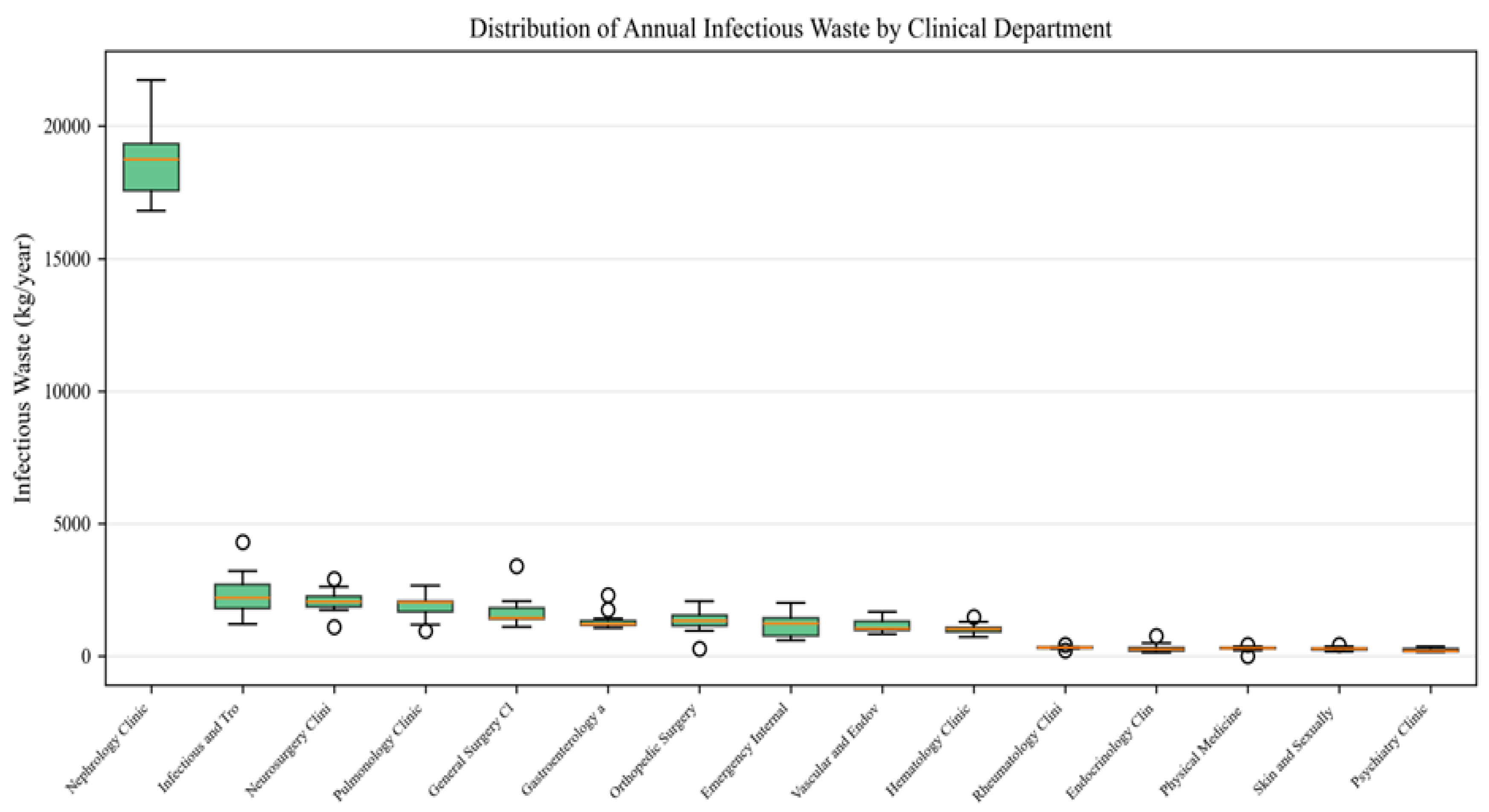
Figure 2.
Annual total infectious waste across all 24 clinical departments in VMA (2011–2021).
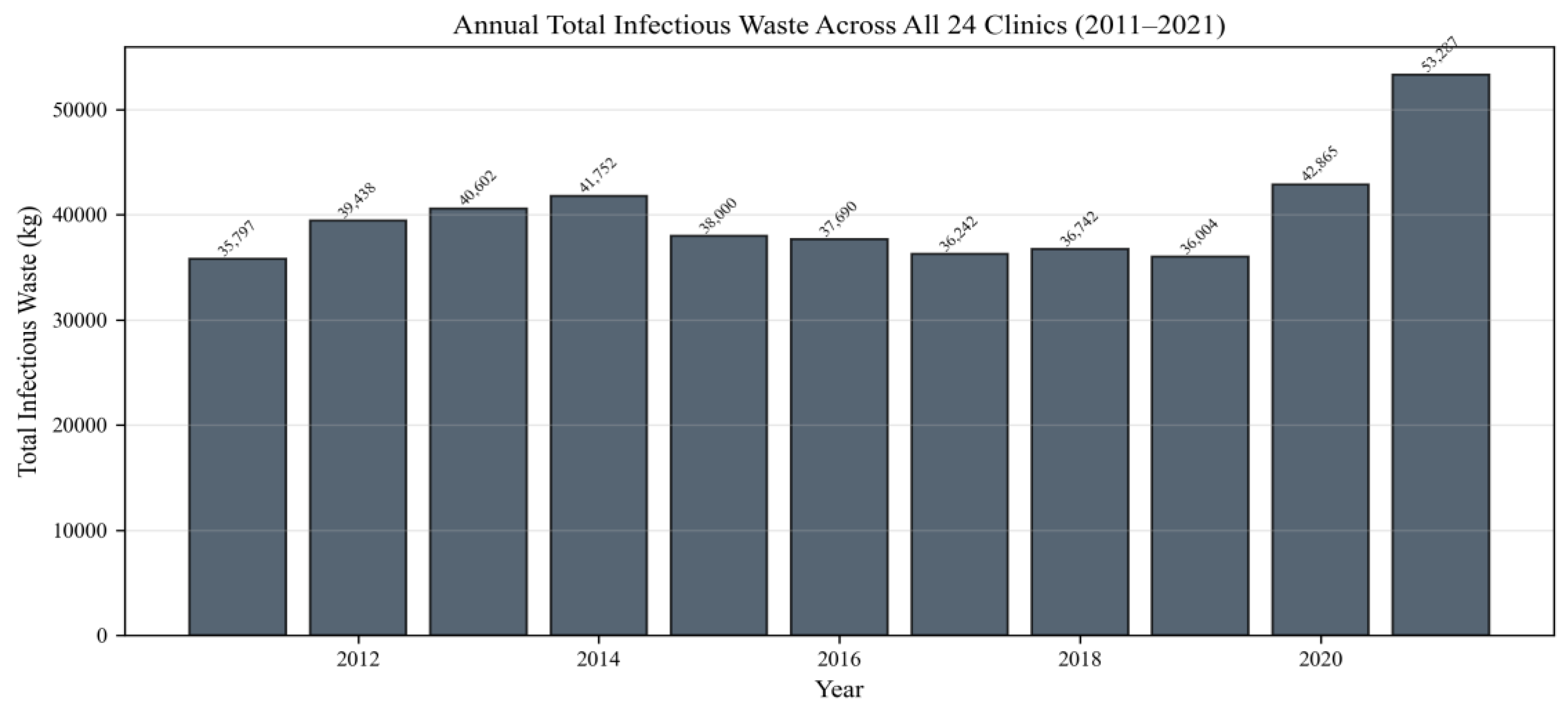
Figure 11.
Aggregate waste forecast (2022–2031) from all six models, plotted against historical actuals (2011–2021). Dashed vertical line marks the forecast boundary.
Figure 11.
Aggregate waste forecast (2022–2031) from all six models, plotted against historical actuals (2011–2021). Dashed vertical line marks the forecast boundary.
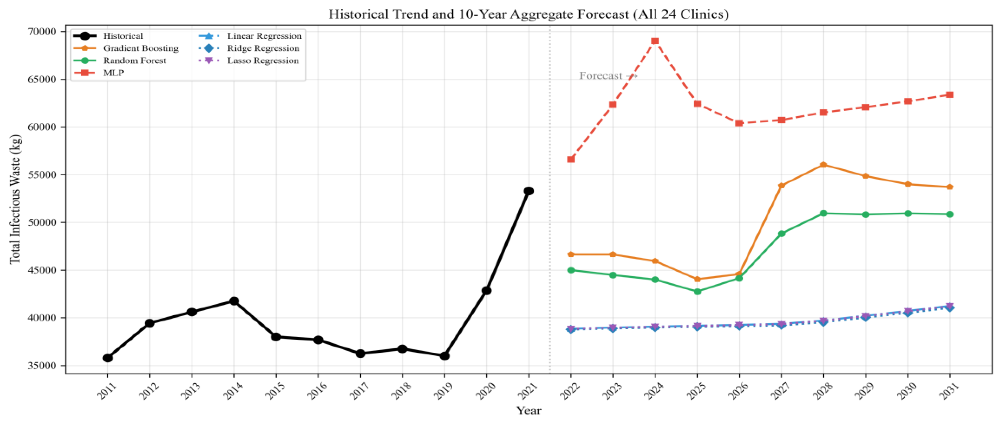
Table 15.
Aggregate 10-year waste predictions (total kg, all 24 clinics).
| Year | GBR | RF | MLP | OLS | Ridge | Lasso |
|---|---|---|---|---|---|---|
| 2022 | 46,632 | 44,998 | 56,573 | 38,844 | 38,760 | 38,825 |
| 2023 | 46,630 | 44,481 | 62,339 | 38,971 | 38,876 | 38,951 |
| 2024 | 45,943 | 44,001 | 69,034 | 39,067 | 38,961 | 39,046 |
| 2025 | 44,037 | 42,746 | 62,429 | 39,164 | 39,046 | 39,141 |
| 2026 | 44,573 | 44,153 | 60,385 | 39,251 | 39,122 | 39,227 |
| 2027 | 53,856 | 48,830 | 60,725 | 39,361 | 39,197 | 39,331 |
| 2028 | 56,045 | 50,954 | 61,517 | 39,709 | 39,531 | 39,678 |
| 2029 | 54,844 | 50,827 | 62,074 | 40,210 | 40,020 | 40,177 |
| 2030 | 53,996 | 50,948 | 62,683 | 40,711 | 40,510 | 40,677 |
| 2031 | 53,704 | 50,858 | 63,379 | 41,241 | 41,035 | 41,204 |
Disclaimer/Publisher’s Note: The statements, opinions and data contained in all publications are solely those of the individual author(s) and contributor(s) and not of MDPI and/or the editor(s). MDPI and/or the editor(s) disclaim responsibility for any injury to people or property resulting from any ideas, methods, instructions or products referred to in the content. |
© 2026 by the authors. Licensee MDPI, Basel, Switzerland. This article is an open access article distributed under the terms and conditions of the Creative Commons Attribution (CC BY) license (http://creativecommons.org/licenses/by/4.0/).
Copyright: This open access article is published under a Creative Commons CC BY 4.0 license, which permit the free download, distribution, and reuse, provided that the author and preprint are cited in any reuse.


