Submitted:
03 April 2026
Posted:
07 April 2026
You are already at the latest version
Abstract
As IoT systems complexity grows, transparent and trustworthy machine-learning Intrusion Detection Systems are crucial. Post hoc explainable AI methods, such as SHAP and LIME, are the most widely used ways to explain how models work, but the degree to which these methods are robust to adversarial conditioning is understudied. In this paper, we propose to create a unified system of evaluating explanation fidelity by using three metrics : sparsity, completeness and robustness based on minimally distorting DeepFool input perturbations. Our study benchmarks SHAP and LIME across three datasets (BoT-IoT, Edge-IIoT, N-BaIoT) using four classifiers: CNN, DNN, LSTM, and RF. Our results demonstrate a consistent trade-off: SHAP achieves stronger causal alignment and higher completeness under attack, whereas LIME exhibits greater rank-stability in terms of top-k feature overlap. However, LIME also produces more spurious attributions and offers less explanatory power than SHAP, especially in the presence of synthetic or non-causal features. Our findings reveal that high model accuracy does not guarantee that the provided explanation is also high-fidelity. This investigation highlights the necessity for robustness-aware XAI in cybersecurity and provides reproducible parameters to guide the adoption of XAI in adversarial environments.
Keywords:
intrusion detection systems
; explainable artificial intelligence
; SHAP
; LIME
; IoT
; sparsity
; completeness
; robustness
; DeepFool algorithm
1. Introduction
The proliferation of Internet of Things (IoT) botnets [1] has changed the security landscape for Internet-attached devices. IoT botnets are a growing concern for the security of homes, businesses, and critical infrastructure. A botnet is defined as a collection of Internet-enabled devices that are controlled by a single entity (botmaster). The botmaster is able to use the botnet for malicious purposes, including distributed denial of service attacks, spamming, and cryptocurrency mining efforts. Due to the number of devices connected to the Internet, the size of botnets of IoT devices can be larger compared to traditional botnets, meaning they are a larger threat to Internet security [2]. Detecting IoT botnets is challenging because they are highly distributed and not confined to any single type of device [1]. IoT botnets exist in such a way that current detection methodologies, like signature-based detection and anomaly-based detection, are not effective. Botmasters can vary the specific behaviors of their IoT botnet quickly to evade detection. Here, the promise of Machine Learning (ML) comes into play as a tactic to detect IoT botnets, given the size of data that can be analyzed and the complexity and patterns in the data itself that are unlikely to be recognized by humans [3,4,5,6].
Despite the myriads of impressive results delivered by many ML methods in the cybersecurity space, there is serious concern due to the intrinsic lack of interpretability of ML models, which means security experts may struggle to trust what an ML model produces because they do not fully understand how a model arrives at a specific decision or classification. Trust is a significant hurdle in intrusion detection systems and many other mission-critical systems. Consequently, a number of novel approaches have been developed in recent years to enhance the explainability of ML models, thereby facilitating more interpretable outputs. This idea is referred to as Explainable Artificial Intelligence in the literature [6]. The assimilation of XAI methods has created a new follow in cybersecurity research to develop and include additional layers of explainability for humans in the loop [7,8]. Several works have considered XAI methods to be useful for IoT botnet detection systems [9,10]. Some survey papers describe current open questions and future research directions [11,12,13,14]. Collectively, these works highlight open issues around standardized evaluation/benchmarks and reproducibility; robustness of explanations under adversarial perturbations and distribution shift; resource-aware deployment on constrained IoT/edge devices; bridging faithfulness vs. plausibility; operational integration with analysts; and privacy security risks from explanations themselves.
Typically, many learned models, like convolutional neural networks, can be treated as “black boxes”, which do not allow verification of the means of decision [15]. Although the purpose of explainable AI is to gain insights into “how” ML models use features; for example, when one is detecting potential IoT botnets, an XAI method can reveal insights into which network features are important in detecting the presence of malicious activity on an IoT device. The information produced by any XAI method is referred to as an “explanation”. Explanations are useful in improving understanding of the models and, along with that, create trust in the decisions made. Model creators and ML scientists can utilize explanations to enhance the model’s performance quality. Furthermore, XAI methodologies can assist in improving a model regardless of whether the explanation is global or local in nature. While global XAI aims to describe the overall behavior of the model, local XAI focuses on explaining individual predictions. It is also relevant to note that in an XAI model, one can achieve explanation using intrinsic (model-specific) XAI, which means that explainability is part of the learning procedure during training of the model (and is not transferable), or via a post hoc (model-agnostic) XAI approach. Post hoc XAI methods are model-agnostic, meaning they do not depend on any specific trained or pre-trained ML model architecture [16].
The rise of XAI techniques, such as Shapley Additive exPlanations (SHAP) [17] and Local Interpretable Model-agnostic Explanations (LIME) [6], seems to emphasize the desperate need for transparent and trustworthy explanations in cybersecurity. Although XAI tools are projected to become a staple of network security, supporting analysts in making decisions more rapidly and accurately, there remains a significant challenge in validating and evaluating these interpreters in real-world Intrusion Detection System settings. Establishing reliable validation procedures and defining security metrics relevant to usability are particularly difficult, as no standardized methods currently exist for assessing the quality and effectiveness of XAI in practical deployments. The extent of validation defines the usability of XAI-based tools but may also hinder the use of AI-based forms of XAI altogether. If there is no standard way to measure and model the utility of the evaluations, it diminishes the usefulness of the security professionals who rely on them for decisions leading to potentially dire consequences [18].
Prior research [19,20,21,22] has established that post hoc explanation methods, such as SHAP and LIME, are susceptible to distortion through adversarial model training, leading to compromised feature attribution and misleading explanations. These previous studies primarily exposed weaknesses in XAI by constructing biased or adversarial models for analysis, but they largely evaluated these models using synthetic attack scenarios. They did not assess explanation methods’ performance against realistic adversarial perturbations, such as those enforced by DeepFool. DeepFool is an adversarial attack method which can minimize perturb inputs to manipulate predictions from the model and modify the input without a loss of the original data’s meaning. It is highly efficient and typically generates adversarial examples that remain very close to the original input. We refer the reader to the original work for a more detailed explanation of the mathematical formulation underlying its iterative procedure [23].
In this paper, we propose a framework for evaluating XAI methods for network intrusion detection systems using various metrics, such as Sparsity, Completeness and Robustess, which are defined as follows:
Sparsity. The sparsity metric measures how concentrated the explanation is on a small subset of features. Given the importance scores assigned by an XAI method, sparsity is evaluated by counting how many features have importance values below a small predefined threshold (i.e., effectively negligible). For example, if 11 out of 19 intrusion features have importance scores close to zero, the remaining 8 features can be regarded as having a strong influence on the model’s decision, indicating a high degree of sparsity in the explanation and allowing security analysts to focus on a reduced set of key traffic metrics.
Completeness. The completeness characteristic of an XAI method is its capacity to provide a correct explanation for any possible network traffic sample. An incomplete XAI method can be exploited by attackers to produce misleading, non-meaningful explanations.
Robustness. The robustness of an XAI method can be defined as the capacity of the XAI method to produce the same explanations with small perturbations of the intrusion features. Such a perturbation can be induced by an adversarial DeepFool attack.
We explore the explainability of the learned model by applying the three evaluation criteria defined above, using two popular black-box XAI methods introduced earlier: LIME and SHAP. Both are well known and regularly used as XAI methods in the network intrusion research domain [24,25,26,27]. LIME provides local explanations to understand how the input contributes to the decision. It builds upon a linear model, where it introduces perturbations to the sample and generates rules about how that model functions on that sample based on those perturbations. SHAP can be considered as both a local and a global explanation method. It evaluates the importance of each feature by determining the corresponding Shapley value for each feature based on the Shapley value concept from game theory [28]. If the output does not change when removing the feature with respect to the original decision of the AI model, then that feature is considered to be of minimal importance with respect to that AI model.
This paper describes the evaluation process step by step for the three-evaluation metrics of sparsity, completeness, and robustness to produce our evaluation metrics and results. We apply our framework to three datasets. The first dataset, BoT-IoT [29], was generated by simulating a realistic network environment at the UNSW Canberra Cyber Range Lab. It includes a mix of normal and botnet traffic. The second dataset, N-BaIoT [30], is associated with the issue of a lack of public botnet datasets available, especially for the IoT, introducing real traffic data collected from 9 commercial IoT devices that were authentically infected by Mirai and BASHLITE. The last dataset, Edge-IIoT [31], was collected from more than 10 types of devices, which included low-cost digital sensors. More details about these datasets are given later, in Section 3.1.
For each dataset, both XAI approaches, SHAP and LIME, will be evaluated across multiple black-box AI models, including Convolutional Neural Networks (CNNs), Deep Neural Networks (DNNs), Long Short-Term Memory networks (LSTMs), and Random Forests (RFs). We then present and analyze the results obtained from the three evaluation metrics computed for each XAI method. This framework aims to broaden the application of XAI within Intrusion Detection Systems (IDS), thereby introducing greater realism to this research area and enabling further advancements.
In addition to the general goal of assessing sparsity, robustness, and completeness using DeepFool as the adversarial model, we highlight the following key aspects of this paper:
- An adversarial stress test that is realistic: A DeepFool perturbation to create perturbations to cross decision boundaries to provide a realistic model of a deceit/adversarial scenario.
- Causally complete assessment: We assess SHAP and LIME top-k based feature explanation against actual feature perturbations by using DeepFool perturbation protocol at the decision boundary to provide an experiential means to attempt to assess explanatory validity under adversarial stress.
- Robustness assessment on the BoT-IoT, Edge-IIoT, and N-BaIoT datasets to compare the stability of SHAP and LIME explanations under adversarial perturbations: We measured how consistently each method preserved its feature attributions before and after DeepFool-based attacks. This allowed us to determine which explainer (SHAP or LIME) produced more robust explanations across the different datasets.
- Introduction of a new perspective on robustness evaluation based on the overlap of top-k feature assessments: Our approach diverges from existing robustness evaluation methods [19], which primarily rely on visual reproductions or simple numerical differences in raw attribution values. Instead, we focus on the semantic integrity of explainability, that is, whether the most important features identified by an XAI method remain stable even when the model is perturbed through adversarial training. For each case, we measure the overlap between the top-k features obtained after applying different perturbation levels using the DeepFool method and the top-k features of the original feature set. This overlap ratio serves as a quantitative measure of robustness.
- Sparsity measures: We provide a review of our sparsity curves to demonstrate how the explanation method ranks features across threshold values.
- Realism and Generalization: Our method provides a dataset-agnostic, attack-focused evaluation, enabling XAI methods to support a scalable framework for IDS and other robustness evaluation tasks.
The remainder of this paper is structured as follows: Section 2 provides a summary of related work. Section 3 details the methodology, including the datasets’ description, the AI and XAI models employed, and the evaluation procedure under DeepFool attacks. Section 4 presents and analyzes the experimental results, and finally, Section 5 concludes the paper.
2. Related Works
As the use of explainable artificial intelligence grows, important questions are arising regarding the reliability and robustness of the post hoc explanation techniques. Important issues in this regard were highlighted by [19], who critiqued popular explanation tools such as LIME and SHAP and demonstrated that these methods can be adversarially manipulated to produce misleading explanations while still yielding correct predictions. The authors noted that a classifier could be adversarially trained to yield the correct prediction while giving misleading explanations, thus being correct but not interpretable. In effect, this demonstrated a serious weakness in some of the existing XAI methods and prompted the research community to work toward more robust and faithful explanation methods.
While building on this weakness, one of the first studies that conducted by [20] systematically reviewed XAI methods in a security-related context. The authors compared several saliency-based methods (e.g., LRP, Grad-CAM, and Integrated Gradients) and applied them to deep learning models for malware classification tasks. The findings from this study revealed that many explanation methods produced unstable and noisy attributions, particularly when inputs were changed very slightly, and the authors cautioned that explanations may often reflect model artifacts rather than any real rationale for the model’s decision. This challenge is especially concerning in consideration of the fact that XAI tools may fail at the very times they are needed most; i.e. in adversarial or other high-risk environments.
Continuing from this work, the TRUST framework proposed in [32] introduces an interpretable IDS for industrial IoT systems using LIME, to encourage transparency. Again, this failed to acknowledge [19] concerns about demonstrating the limitations of early-stage explainability frameworks in adversarial settings.
In 2022, these limitations were also addressed by [33] who proposed a framework that employed SHAP and RuleFit as add-ons on top of DNN for IoT IDS using the NSL-KDD and UNSW-NB15 datasets. While their approach enhanced interpretability by incorporating adversarial attacks, the framework was computationally expensive, highlighting the common trade-off between robustness and efficiency. [24] developed detection accuracy on large-scale IoT data by using SHAP with ensemble models (random forest/decision trees) to improve general interpretability. However, their approach was not applied to more recent and richer deep learning architectures. At the same time, LIME with ensemble classifiers was also used in [34] for improved interpretability and explained that they did not assess performance in high-velocity data streams, a key feature for real-time IDS systems.
In 2023, the XAI community began to advance to evaluation-based works, related to benchmark creation and quantitative evaluation. A dataset collection of comprehensive visual explanation studies (e.g., Gender-XAI, Nodule-XAI) was created by [35] and provided the evaluation of three methods, Grad-CAM, RISE, and ViT. Significant contributions were made [35] toward establishing a much-needed standard for evaluating XAI methods. However, they also identified challenges associated with using human-annotated data, such as the presence of biases, and raised concerns about whether models may have inadvertently exploited other datasets or spurious features. Such issues could undermine generalizability and fail to capture true task-specific similarities. In 2023, an interpretable fuzzy decision tree-based IDS for IoT networks was created by [36], which is an inherently interpretable (explainable) alternative, but the work was very preliminary and without an external validation study.
A real-time IDS using SHAP with a Random Forest model [37] was successfully implemented on the UNSW-NB15 dataset; however, the evaluation relied on this single dataset, limiting the validity and generalizability of their findings. In 2023, MEMC, a new XAI evaluation metric, was proposed by [38] and focused on healthcare XAI model interpretability. However, they also did not capture the computational costs specific to high dimensionality. Finally, completeness and correctness of explanation with LIME using multiple datasets were provided by [39], exposing dependencies on human feedback and classifier performance.
By 2024, the discussion and overall concern of evaluation metrics had a wide scope of maturity, and the Mean Opinion Score (MOS) [40] was validated as a user-driven measurement, showing only a weak correlation with other symptoms of automatic measures such as IAUC and DAUC, acknowledging the limitation of the subjective layer of example or explanation evaluation being unaddressed. Also in 2024, sMPRT and eMPRT frameworks were proposed by [41] as a structured way to engage in the evaluation of explanation mimicry and model complexity. While their extensibility is evident, the frameworks appear markedly complex and computationally expensive, both in terms of processing requirements and the interpretative challenges of inductive tasks, particularly given the extensive groundwork needed to establish evaluation metrics.
Wrapping up this line of research, [21] introduced a comprehensive framework for evaluating black-box explanation techniques, particularly SHAP and LIME, in intrusion detection systems, considering both global and local perspectives across multiple IDS datasets. In a parallel direction, [22] extended a similar evaluation philosophy to anomaly detection in autonomous driving systems and explicitly assessed SHAP and LIME across six evaluation metrics, including sparsity, completeness, and robustness. Together, these studies established an important foundation for examining explanation quality beyond predictive accuracy alone. However, they still leave open a critical question for adversarially exposed environments: how explanation fidelity should be assessed when explanations are stressed by minimal, decision-boundary-crossing perturbations rather than only by broad evaluation criteria.
Building on these foundations, our work provides a more adversarially grounded and application-specific evaluation of SHAP and LIME in IoT intrusion detection. More specifically, our methodology differs from [21,22] in the way completeness and robustness are operationalized. For completeness, instead of relying on a general explanation-quality criterion, we use a DeepFool-based feature-alignment formulation in which the original top-k features identified by SHAP or LIME are compared against the input dimensions perturbed along the minimal adversarial path, producing completeness curves . For robustness, rather than adopting a single generic robustness score, we evaluate explanation stability through three complementary tests: (i) a clean-versus-adversarial explanation comparison under DeepFool, (ii) a synthetic unrelated-feature test to reveal spurious attributions, and (iii) a top-k feature-overlap analysis with paired t-test and Wilcoxon signed-rank validation. In this sense, our study remains aligned with the recent state of the art while offering several concrete advances: a unified and reproducible framework across three IoT IDS benchmarks and four classifiers, a more fine-grained adversarial analysis of explanation behavior, and a clearer characterization of the trade-off between causal faithfulness and rank-stability under adversarial conditions. Consequently, the contribution of this work is not limited to predictive performance, but lies in delivering a more realistic and operationally relevant assessment of explanation fidelity in adversarial IoT environments.
3. Methodology
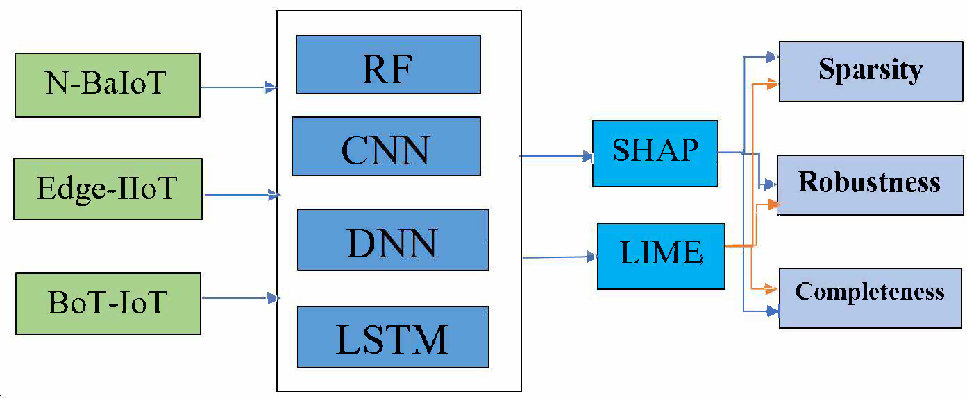
This section explains the experimental design incorporating explainable AI techniques with adversarial experiments across several network intrusion detection datasets and machine learning models (see Figure 1). The approach is implemented to evaluate explanation in terms of sparsity, completeness, and robustness under DeepFool attack conditions.
3.1. Datasets Description
We employed three publicly available intrusion detection datasets:
BoT-IoT [29]: The BoT-IoT dataset was generated whilst using the Ostinato tool to generate network traffic data from a cloud server using virtual machines and Kali Linux machines running various services; these services included DNS, SSH, FTP, and HTTP. The Kali machines simulated the IoT devices in the experiment, and Node-RED was used as the programming tool to enhance the realistic behavior of each IoT device. The dataset includes 5 different IoT scenarios, with each scenario representing a different IoT device (weather station, smart refrigerator, motion-activated lights, remotely activated garbage door, and smart thermostat). The network traffic data that was collected contained several types of attacks that included UDP, TCP, OS fingerprint, service scan, HTTP, keylogging, and data exfiltration. The dataset is provided in two versions: a full version containing over 72 million records and a 10% version with approximately 3.6 million records. In this study, we evaluate the proposed model using 5% of the full dataset, focusing on the optimal feature set.
N-BaIoT [30]: For the N-BaIoT datasets, attacks are performed using C&C (Command and Control) servers, which are used by botmasters to control a network of infected IoT devices (bots). The C&C server is the microsystem, which the botmaster uses to send commands to the bots and receive information the bots send back. The N-BaIoT dataset used Mirai and Gafgyt botnets to deliver malware and execute coordinated DDoS (Distributed Denial of Service) attacks. These botnets delivered malware to various IoT devices, including routers, cameras, and other smart devices, by exploiting various vulnerabilities. The N-BaIoT datasets include features recorded in this controlled testing environment. The datasets contain combined statistics of the raw network streams, over five different time windows (100 ms, 500 ms, 1.5 s, 10 s, and 1 min), with 115 features obtained from the network traffic. The time windows are coded L0.01, L0.1, L1, L3, and L5, respectively. Each feature is assigned to five main categories of metrics, with the categories including: host-IP(H), host MAC&IP (MI), channel (HH), socket (HpHp), and network jitter (HH_Jit). The statistical values used from the five higher-order metrics: the number of packets, the mean, and the variance of packet sizes. The channel and socket categories have additional values derived from packet size, radius, covariance, and magnitude, such as the correlation coefficient.
Edge-IIoT [31]: This dataset consists of data collected from more than 10 types of devices, including low-cost digital temperature and humidity sensors, pH meters, ultrasonic sensors, heart rate sensors, water-level detectors, soil moisture sensors, flame sensors, and similar equipment. In this database, there are 14 different kinds of attacks with IoT and various IIoT protocols: MITM, Fingerprinting, Ransomware, Uploading, SQL injection, DDoS_HTTP, DDoS_TCP, DDoS_UDP, DDoS_ICMP, Password, Port Scanning, Vulnerability Scanner, Backdoor, and XSS.
Each dataset was preprocessed using standard techniques, including label encoding and class balancing. We used 80% for the training stage and 20% for the testing stage. We did utilize all the features listed in Table 1 in our initial experiments. This comprehensive approach allowed us to fully leverage the datasets for our analysis of network intrusion detection. Table 1 summarizes the overall scope of each dataset, including the number of features, the number of labels, and the number of samples.
3.2. Machine Learning Model
We trained and assessed four black-box classifiers that are commonly used in the IDS community:
RF: Using Scikit-learn, the random forest classifier was built with a set of hyperparameters that were similar for all three datasets to ensure a controlled and comparative evaluation. Each model used 100 decisions trees, minimal depth of 5 samples per leaf, maximum depth of 15, and minimal 10 samples required to divide a node. These parameters were selected based on initial trials to balance the variance and bias in the dataset with different feature dimensions. By maintaining the same hyperparameters, we ensured that any performance differences we viewed were due to dataset and not amending the model configuration.
DNN: The architecture used in this research utilizes the Keras Sequential API and is designed to classify intrusion detection datasets. The architecture of this classifier receives as input a feature vector whose length matches the number of features in the dataset, and feeds it into an initial input denes layer with 128 neurons using the rectified linear unit (ReLU) activation function, which is used for all datasets. Then there is a larger Dense hidden layer with 256 neurons (with ReLU activation) that also uses L2 regularization (l2(0.001)) to penalize large weights and control overfitting. A Dropout layer follows, in which 10% of the neurons were randomly dropped out in training to enhance generalization. Next, the model contains another Dense layer of 64 neurons to continue the feature learning process, which also utilizes L2 regularization. The output Dense layer contains several neurons equal to the number of classes for each dataset and a softmax activation function, which provides a probability distribution over target classes. The loss function was configured to use “categorical crossentropy," while the adaptive momentum Adam was chosen as the optimization algorithm [42].
CNN: The classification model employed within this study is based on a convolutional neural network architecture using Keras’ Sequential API. The network starts with a Reshape layer, which transforms the input into a 4D tensor of shape (features, 1, 1) to make use of the 2D convolutional layer. This is followed by a Conv2D layer with 64 filters of kernel size (1,1) and ReLU activation to introduce non-linearity. The output of the Convolutional layer is then flattened into a 1D vector using a Flatten layer. Next, a fully connected dense layer with 32 units and a ReLU activation function is applied to extract high-level feature representations. The final layer is a Dense layer with units equal to the number of classes for each dataset and softmax activation for a probability distribution over the output classes corresponding to each dataset class. This model is overall designed to process tabular intrusion detection data with a CNN-based feature extraction.
LSTM: A recurrent model for perceived sequence-like representations of traffic windows. The classification model based on LSTM and employed in this work was built using the Keras Sequential API to process historical tabular data as sequential representations of network traffic. The LSTM model starts with an LSTM layer, which is set up to take an input shape of (n_feats, 1), with n_feats being the number of features in the case. After the LSTM layer, several fully connected dense layers were added, with the number of neurons increasing progressively across the sequence: 20, 60, 80, and finally 90 units. A linear activation function was used by default, allowing the model to gradually build more complex and hierarchical feature representations.The final output layer is a dense layer with a number of units equal to the number of classes in each dataset, and it uses a softmax activation function to produce a probability distribution over the target classes.
3.3. XAI Methods
As previously introduced, two post-hoc explanation methods, LIME and SHA, have been employed to explain the decisions of the trained model.
LIME approximates the decision boundary of a complex model using an interpretable surrogate model for a specific prediction. For each test case, LIME draws perturbed samples in the neighborhood of the data and observes the output generated by the classifier. The perturbed samples and outputs from the classifier are then fit with a sparse linear model to the samples to find the most important features that generated the prediction. The method allows us to extract feature attributions for individual predictions without requiring access to the model’s internal architecture.
SHAP is a unified approach based on cooperative game theory, which assigns each feature a value called the Shapley value representing its contribution to the prediction. SHAP guarantees consistency and local accuracy, meaning that feature attributions faithfully reflect the model’s behavior for individual predictions. Unlike LIME, SHAP provides additive attribution across all input features, offering a theoretically grounded explanation of why the model produced a particular prediction. This approach also supports global consistency, making it easier to interpret overall model behavior. For all test cases, SHAP values were computed using KernelExplainer or DeepExplainer, depending on the model type.
We choose SHAP and LIME for our pipeline because they can overcome the limitations of single-feature explanation techniques such as Leave-One-Column-Out (LOCO)[43], Individual Conditional Expectations (ICE) [44], and Partial Dependence Plots (PDP) [45]. For intrusion detection jobs where dependencies among network traffic attributes are critical, these approaches are useful for global or marginal effects, but they cannot capture complex interactions between several features. However, SHAP and LIME provide locally faithful feature-level explanations that preserve instance-level model fidelity while accounting for these interactions. Their selection as dependable and trustworthy criteria for evaluating the robustness, completeness, and sparsity of explanations is further supported by their widespread use and demonstrated effectiveness in IDS-related work.
3.4. XAI Evaluation Metrics
The quality of explanations is evaluated using three primary metrics: sparsity, completeness, and robustness. Each metric offers a different perspective on how reliable and interpretable the explanations are under adversarial perturbations. Next, we describe each metric in detail and how it is measured within our evaluation framework.
Sparsity: We assess the degree of sparsity for each AI model using Cumulative Thresholded Sparsity (CTS) curves created from LIME and SHAP for each of the three datasets. The feature importances on a scale from 0-1. At a given threshold value, CTS is defined as the fraction of features with importance less than or equal to that threshold relative to the total number of features. Therefore, the CTS curve at any threshold shows the cumulative distribution of feature importance scores. A very sparse explanation would have a high CTS curve at a low value of the x-axis, demonstrating that many features have low importance but only a select few high importance features contribute most of the importance score; in this scenario, the CTS curve would rise very quickly to near 1 and remain there for those low threshold values. When there is a relative even distribution of importance scores among several features, however, the CTS curve will exhibit a more gradual increase in comparison to tall bars on a histogram. The Area Under the Curve (AUC) was computed using the trapezoidal rule, where higher CTS-AUC numbers indicate greater sparsity and concentrated explanations, while lower CTS-AUC numbers indicate less sparsity and more dispersed explanations. This is done using the following process:
1.- Compute raw importance scores for all features of a given instance using LIME and SHAP.
2.- Apply min-max normalization to make the feature-importance values a digit between [0, 1]. This ensures that all feature scores lie within the same interval, preventing any feature from being disproportionately weighted simply due to its original scale.
3.- Create a list of thresholds from 0 to 1 in increments of 0.1, and for each threshold , count how many normalized feature scores satisfy:
4.- At each threshold, compute the CTS score using the following equation:
5.- Repeat Steps 3 and 4 for all values in the threshold list (0.0 to 1.0) and plot the CTS curve where the x-axis represents the threshold and the y-axis represents CTS().
6.- To quantitatively summarize the curves generated in Step 5, compute CTS-AUC using the trapezoidal rule. The resulting CTS-AUC summarizes the sparsity of the explanation: higher values indicate sparser, more concentrated explanations, whereas lower values indicate less sparse, more diffuse explanations.
Completeness: The definition of Completeness given here refers to the percentage of input dimensions that an XAI method highlights as having a significant impact on the prediction made by the model. To test the Completeness of the SHAP and LIME post hoc methods in an adversarial setting, we use a phrased DeepFool framework to test how similar the most critical features of the input sample identified by the explainer are to those input dimensions that require perturbation by DeepFool for class alteration by the model. For a provided input sample x , we follow the following series of steps:
1.- Compute the top-k most important features for the unperturbed x input using SHAP or LIME; we interpret these as an explanation of the model’s decision and denote their indices by.
2.- Use the DeepFool algorithm to compute a minimal adversarial perturbation vector in the input feature space such that the model prediction changes, i.e., . The vector has the same dimension as x, so each input feature can be modified by a different amount.
3.- Define intermediate perturbation levels: , where in steps of 0.1.
4.- At each perturbation level , identify the set of features whose values have changed with respect to the original input x. We denote this set by ; these features represent the model’s vulnerable decision dimensions at that perturbation level.
5.- For each scaled perturbation , check whether the top-k features from the original explanation overlap with the features perturbed by DeepFool. We say that there is overlap at level if
6.- Repeat the assessment process over many samples for each attack class, and compute the proportion of samples in which at least one of the top-k features coincides with the perturbed features by DeepFool. This produces completeness curves, showing how well the XAI method’s top-k features align with causally relevant input dimensions as the perturbation levels increase.
Where:
= set of top-k features in the XAI explanation for the original sample .
set of features perturbed by DeepFool at perturbation level .
=indicator function (1 if true, 0 if false).
N = number of samples tested.
= scaled perturbation magnitude .
Robustness: Robustness in XAI refers to the stability of feature attributions when inputs are subjected to adversarial perturbations. A robust explanation method should preserve its most influential features even when the model’s inputs are minimally manipulated. To systematically assess robustness, we employed the DeepFool attack as our adversarial perturbation method and evaluated the stability of SHAP and LIME explanations across three complementary tests.Although both completeness and robustness are evaluated using DeepFool and top-k features, they capture different properties: completeness checks whether the features highlighted by the XAI method are truly causal for the prediction, whereas robustness measures how consistently the top-k features and their ranking are preserved under minimal but decision-changing perturbations.
Test-1 Robustness without Injected Feature Bias: In this evaluation, we investigate robustness of SHAP explanations when the model is subjected to minimal adversarial perturbations. For each clean test instance, we compute SHAP values for the predicted class and select the top-k most important features, which act as the baseline explanation. We then apply the DeepFool algorithm to generate adversarial examples with minimal perturbations that change the decision of the model. We again apply SHAP to these adversarial examples to generate a new ranking of top-k features. Finally, we compare the explanations for clean and adversarial inputs to analyse how well the top features are preserved under an adversarial perturbation. Mathematically, let be the trained classifier, and be the predicted class for input x. The SHAP attribution vector for x with respect to is:
The minimal adversarial perturbation is obtained from DeepFool by solving the following :
The adversarial sample is: . The SHAP attribution vector after attack is:
Then, we perform a qualitative or list-based comparison between and to evaluate attribution stability under adversarial perturbation.
Test-2 Robustness under Biased Feature Influence: In this evaluation, we examine how XAI methods behave when the model is trained with a deliberately injected spurious feature. Specifically, we introduced a synthetic, unrelated feature u into the dataset prior to training. This gives the opportunity for the model to attribute spurious feature importance to u. For each clean test instance, we compute SHAP or LIME values to obtain the baseline top-k feature ranks. We then apply the DeepFool algorithm to generate adversarial perturbations of the clean test instances and subsequently re-compute the top-k features using SHAP and LIME on the perturbed inputs. By comparing the ranks of the original test instances and perturbed test instances, we determine whether the spurious feature became the dominant feature in the explanation under adversarial perturbations, therefore demonstrating a robustness failure.
Mathematically, let the feature set be where u is the injected unrelated feature. SHAP/LIME attribution vectors:
and top-k feature sets: . Robustness under bias is compromised if: and , showing that the spurious feature becomes overly dominant due to adversarial perturbation.
Test-3 Top-k Feature Overlap: The third robustness evaluation measures the consistency of feature attributions produced by SHAP and LIME before and after adversarial perturbation. Specifically, we assess whether each explanation method can maintain stable top-k feature rankings when subjected to input-level attacks that do not significantly change the underlying semantics of the data. For each dataset (BoT-IoT, Edge-IIoT, and N-BaIoT), we randomly selected 100 test samples. We applied SHAP and LIME to each original sample to extract the top-10 most important features. The input sample was then perturbed using the DeepFool algorithm, which generates minimal adversarial changes required to cross the model’s decision boundary. SHAP and LIME were again applied to the adversarial version of each sample to retrieve a new top-10 feature list. We computed the Top-k overlap ratio for each sample as the number of features common to both original and adversarial top-10 sets, divided by 10. This overlap ratio ranges from 0 (wholly distinct explanations) to 1 (same attributions). The average overlap over all 100 samples was calculated for each method and dataset. We also computed the 95% CI for the mean overlap scores to assess the correctness. Finally, we used paired t-tests and Wilcoxon signed-rank tests to quantitatively assess the robustness difference between SHAP and LIME. The paired t-test assumes that the differences between paired scores are approximately normally distributed, whereas the Wilcoxon signed-rank test does not require normality and is more appropriate when the distribution of differences is skewed or contains outliers. By applying both tests, we account for potential violations of the normality assumption and obtain a more reliable comparison of the two XAI methods. In this analysis, a higher mean overlap with narrower confidence limits indicates greater explanation stability under adversarial disturbance. Mathematically, let:
,
The overlap ratio is:
The robustness score across a dataset of N samples is the mean overlap:
Then, compute the sample standard deviation:
The 95% CI is: , where is the critical value of Student’s t distribution with N-1 degrees of freedom. We compare SHAP vs LIME robustness scores across the same N samples.
Let the differences be:
compute the mean difference and the standard deviation of differences: Assuming are approximately normal, we use the paired t-test and compute:
For the Wilcoxon signed-rank test, for each pair, compute the difference , remove zero differences, rank the absolute differences from smallest to largest, assign signs according to the original , and compute the signed rank sums:
The test statistic is:
In general, this framework evaluates robustness in a three-tier system:
Test-1 the qualitative stability of the explanation is assessed at the sample level through visual inspection to determine if the most salient features remain unchanged (or substantially different) between clean and adversarial explanations.
Test-2 investigates how sensitive explanation methods are to the introduction of spurious features and whether they will highlight spurious features that contain no information when adversarial noise is added.
Test-3 quantitatively determines the robustness of the explanation by calculating the overlap ratio (taking the top-k features) between clean and adversarial explanations, across many samples, as well as calculating a numerical stability score that will be statistically validated using paired t-tests and Wilcoxon signed-rank tests.
4. Results and Discussion
4.1. Results of Sparsity Metric
We provide and discuss the findings of our sparsity assessment for SHAP and LIME explanations across three IoT intrusion detection datasets, BoT-IoT, Edge-IIoT, and N-BaIoT. The Cumulative Threshold-Based Sparsity Curves for LIME and SHAP can be seen in Figure 2, Figure 3 and Figure 4, which indicates how feature importance scores using LIME and SHAP are spread out for each dataset as a function of a series of increasing thresholds () ranging from 0 to 1 in steps of 0.1 and thus can be interpreted as a cumulative histogram of the feature scores. A CTS curve that rises quickly and remains close to one for relatively small thresholds indicates a sparser, more concentrated explanation, whereas a CTS curve that grows more gradually indicates a less sparse, more diffuse explanation.
For the BoT-IoT dataset, the CTS curves in Figure 2(a) (LIME) and Figure 2(b) (SHAP) reveal clear differences in how sparsely each XAI method distributes importance across features. In Figure 2(a), the LIME curves, especially for the CNN and LSTM models, rise rapidly and remain close to one, indicating very sparse explanations in which a small subset of features dominates the attribution and many potentially informative signals are largely ignored. In contrast, the SHAP curves in Figure 2(b) generally grow more gradually, reflecting explanations that are still relatively concentrated but spread importance over a broader set of features. These visual trends are supported by the CTS-AUC values in Table 2. For the DNN and RF models, SHAP attains slightly higher CTS-AUC values than LIME (0.623 vs. 0.436 for DNN, and 0.625 vs. 0.607 for RF), indicating somewhat sparser yet still balanced explanations. For the CNN and LSTM models, however, LIME yields markedly higher CTS-AUC values than SHAP (0.671 vs. 0.450 for CNN and 0.693 vs. 0.500 for LSTM), confirming that LIME produces extremely sparse explanations that collapse onto a few dominant features. Overall, while both XAI methods are applied to highly accurate BoT-IoT classifiers, SHAP provides more balanced explanations over several relevant traffic features, whereas LIME, particularly for CNN and LSTM, tends to oversimplify the decision rationale by concentrating importance too narrowly. For the N-BaIoT dataset, the CTS curves in Figure 3(a) and Figure 3(b) show a more mixed sparsity pattern than in BoT-IoT. In Figure 3(b), the SHAP curves for the DNN and CNN models rise rapidly and remain close to one over a wide range of thresholds, indicating highly concentrated explanations in which a small subset of features dominates the attribution. In contrast, the corresponding LIME curves in Figure 3(a) grow more gradually, suggesting less sparse, more diffuse explanations for these models. This behaviour is consistent with the CTS-AUC values in Table 2, where SHAP achieves higher AUC than LIME for DNN (0.812 vs. 0.684) and CNN (0.832 vs. 0.655), reflecting more concentrated SHAP attributions in these two cases. For the RF model, the situation reverses: LIME attains a higher CTS-AUC than SHAP (0.765 vs. 0.559), indicating that LIME is more sparse and tends to collapse the explanation onto fewer features, while SHAP distributes importance more broadly. For LSTM, both methods exhibit similar CTS-AUC values (0.679 for SHAP vs. 0.682 for LIME), so neither shows a clear advantage in terms of sparsity. Overall, these results suggest that, on N-BaIoT, SHAP often provides concentrated yet structured explanations for DNN and CNN, whereas LIME can become overly sparse for RF, potentially overlooking subtler but still informative feature contributions.
For the Edge-IIoT dataset, the CTS curves in Figure 4(a) and Figure 4(b) again highlight clear differences in how feature importance is distributed across models. In Figure 4(a), the LIME curves show a noticeable rise at lower thresholds (between 0.1 and 0.3), particularly for the DNN and LSTM models, indicating that LIME concentrates part of its attribution on a subset of features while still assigning non-negligible importance to a wider set. By contrast, the SHAP curves in Figure 4(b) increase more sharply and remain close to one across a broader range of thresholds for all four models, especially CNN and RF, reflecting more strongly concentrated, highly sparse explanations in which a small group of features dominates the attribution.These visual patterns are confirmed by the CTS-AUC values in Table 2. SHAP consistently attains higher AUC values than LIME across all models—DNN (0.929 vs. 0.778), CNN (0.921 vs. 0.537), LSTM (0.931 vs. 0.729), and RF (0.763 vs. 0.609)—indicating that SHAP produces systematically sparser explanations on Edge-IIoT. While this strong sparsity enables SHAP to highlight a compact set of highly influential features, it also increases the risk of overlooking additional, more subtle signals that may contribute to the classifier’s decisions. In contrast, LIME yields less sparse, more diffuse explanations that distribute attribution more broadly, which may better reflect the complex structure of Edge-IIoT but at the cost of reduced conciseness and a higher cognitive load for analysts who must interpret a larger set of contributing features.
Taken together, the CTS curves and CTS-AUCs tell us a lot about how SHAP and LIME perform when used across all three types of IoT (BoT-IoT, N-BaIoT, and Edge-IIoT). In most setups (especially for DNN and CNN, and clearly on Edge-IIoT), SHAP produced much higher CTS-AUC than LIME; also, SHAP produced much steeper CTS curves than LIME. The resulting explanations from SHAP were mainly comprised of a limited number of features that accounted for a disproportionate share of the reasoning behind SHAP’s predictions. SHAP is more useful for identifying important traffic indicators while possibly ignoring some of the nuanced signals that would be helpful in the decision-making process. Conversely, LIME had much lower average CTS-AUC than SHAP; and, LIME produced much flatter CTS curves than SHAP. Therefore, LIME’s explanations were typically made up of a significantly greater number of features than SHAP. However, on occasion, LIME’s explanations would become significantly sparse, with only a few dominant contributors to the prediction.
The overall outcome of this research is that SHAP can offer a relatively structured high-sparsity explanation that can allow use as a clearer indicator of feature importance, while LIME can provide a useful alternative in that it provides a more evenly distributed view of a broader number of contributors. The above findings confirm that predictive accuracy will not always correlate with the degree of explanation provided, and that the sparsity and distribution characteristics of the XAI approach should be evaluated together with performance metrics of IoT intrusion detection.
4.2. Results of Completeness Metric
Evaluating completeness involves evaluating how much explanation methods (LIME and SHAP) capture the truly influential features that were affected by the adversarial perturbations. This study examines perturbations induced by DeepFool from varying levels of intensity across three different IDS datasets with a number of samples equal to 100. We show the results of the experiment in Figure 5, Figure 6 and Figure 7.
As shown in Figure 5(a), SHAP appears to have a higher degree of completeness on the BoT-IoT dataset. As the intensity of DeepFool perturbation () increases, the top-k features of SHAP also begin to increasingly overlap with the true feature perturbations. This suggests that SHAP can more reliably discern the causally relevant features, and its explanations degrade gracefully concerning the adversarial perturbed input. Early overlaps between SHAP’s explanations and the features perturbed by DeepFool suggest that SHAP is predicting in line with the model’s decision boundary under the stress of the perturbation. In stark contrast, LIME shows in Figure 5(b) significantly reduced completeness on the BoT-IoT dataset. Even as increases, the top-k LIME features rarely appear in the features that DeepFool perturbed. This indicates a mismatch between LIME’s explanations and the model’s actual decision-making based on the features. Although LIME maintains an air of stability under small perturbations, this is potentially deceptive, since the features of the model’s true causal paths are absent, which jeopardizes LIME’s trustworthiness in consequential IDS scenarios.
Although N-BaIoT is a more sensitive dataset, with class predictions changing rapidly under small DeepFool perturbations, SHAP still has relatively high completeness (see Figure 6(a)). A better indication, however, is that its top-k features still meaningfully overlap with perturbed features at each level of , indicating that SHAP explanations still remain partially valid even under model instability. This further demonstrates that SHAP is robust to capture causally influential features. In Figure 6(b), LIME completely fails to track the changing causal structure of the model under perturbations. Top-k LIME features do not match DeepFool perturbation features consistently, and there is significant causal fidelity loss. Even more concerningly, even when the prohibition prediction was different LIME explanation still focused on irrelevant features and static features.
For the Edge-IIoT dataset (Figure 7(a)), SHAP demonstrates relatively high completeness, with its top-k feature attributions increasingly overlapping with the features perturbed by DeepFool as the perturbation intensity () grows. This indicates that SHAP explanations are generally aligned with the model’s decision boundaries under stress. However, when comparing across datasets, it appears that N-BaIoT reaches higher completeness levels earlier (at lower perturbation scales), whereas SHAP’s completeness for Edge-IIoT grows more gradually. In contrast, LIME (Figure 7(b)) remains less consistent: its top-k features show limited alignment with the perturbed dimensions, particularly at lower values, suggesting that LIME struggles to capture the causally relevant features as perturbations increase.
As a summary, the completeness results illustrate the degree of equivalence of LIME and SHAP explanations to the true feature perturbations performed by the DeepFool adversarial attack on the examined IDS datasets. The perturbation intensity progressed from none to full scale and overlapped with the top-k features from each explanation method, and the ground-truth perturbed features varied from none or single overlaps to majority overlaps. SHAP consistently showed increasing overlap across all perturbation intensities, with a steady and moderate rise in feature perturbation completeness under adversarial stress. This indicates that SHAP is more robust than LIME in identifying relevant features when the model is subjected to adversarial perturbations. Further, LIME had reduced overlap counts and exhibited variable overlap counts that are more appreciated at the moderate perturbation intensity, meaning LIME could be especially sensitive to perturbations and struggles to maintain completeness of explanation. These results have implications for understanding the trustworthiness of post-hoc explanation methods in areas that are security-critical and that are also facing adversarial attacks.
4.3. Results of Robustness Metrics
Test-1: We evaluate the robustness of SHAP under adversarial contexts with the DeepFool attack as our adversarial perturbation method before and after the application of the attack on the three analyzed datasets, as shown in Figure 8, Figure 9 and Figure 10.
Figure 8 shows SHAP explanaitions for the BoT-IoT dataset before and after being attacked by DeepFool, revealing that there was a large and considerable shift in feature attribution after the application of an adversarial attack. As illustrated in Figure 8(a), the original SHAP explanation was composed mostly of small clusters of traffic-related variables that accounted for the largest portion of the model’s reasoning (i.e., maximum flow values, Data Rate, and Number of Inbound Connections). After attacking the SHAP explanation using DeepFool, a new set of variables are present as shown in Figure 8(b), which is comprised of a collection of state and address descriptors, among other statistical variables. Many of the previously dominant features that were included in the original dataset have lost significance since their ranking decreased after having been replaced with new features. These results show that the SHAP explanation is very sensitive to small perturbations in the input without any changes to either the architecture of the model or to how it was trained.
The SHAP explanations for the second dataset, Edge-IIoT shown in Figure 9 , show significant alteration in the feature importance ranking due to the adversarial perturbation caused by DeepFool. As seen in Figure 9(a), before the attack occurred, the most influential features pertained primarily to transport and application layers, including aspects of TCP segment length and flags, in addition to MQTT header data. Collectively, these factors represent domain-relevant stimuli, demonstrating that the model relies on behavioral characteristics at the protocol level to differentiate traffic patterns. However, after implementing the perturbation from DeepFool, as indicated in Figure 9(b), a few of the protocol-related features remain among the highest ranked; however, the rankings and importance of those protocol variables noticeably change. In fact, many of the application layer attributes previously deemed most influential lose significance; conversely, several features in the transport layer and connection-oriented domains become more prominent in the SHAP Explanations. Overall, the rank change in feature importance, combined with the Predicted Class remaining the same, illustrates that DeepFool can alter the internal decision process of the model, despite an apparent similarity of the broad set of influential features. For Figure 10, the SHAP explanations on the N-BaIoT dataset show a moderate but meaningful change in feature importance after the DeepFool perturbation. In Figure 10(a) , the highest-ranked variables correspond to statistical descriptors of traffic behaviour (e.g., measures related to variance and weighted frequency), indicating that the model relies strongly on structured, frequency-aware characteristics of IoT traffic for anomaly detection. In Figure 10(b), some of these statistical descriptors remain among the top features, but their relative importance changes, and several previously lower-ranked descriptors move up in the ranking. Overall, this partial reshuffling suggests that, beyond merely flipping the model’s prediction, the underlying reasoning of the classifier is altered by the adversarial perturbation, thereby compromising the consistency of local explanations.
Test-2: With a fake unrelated feature, we evaluate the robustness of SHAP and LIME under adversarial contexts with the DeepFool attack as our adversarial perturbation method before and after applying the attack on three datasets, as shown in Figure 11, Figure 12 and Figure 13.
In the evaluation of robustness within the BoT-IoT dataset, SHAP maintains considerable stability and is more robust in its feature attributions when compared to LIME in the presence of adversarial perturbations (see Figure 11(a) and Figure 11(b)). As discussed earlier, both methods initially identified the core features of the model completely; however, following perturbation using DeepFool, we see LIME’s explanations are altered extremely. In Figure 11(c) for LIME explanation,the injected synthetic feature appears at the top of the importance ranking, despite being explicitly designed as unrelated to the underlying classification task, which makes its prominence in the explanation difficult to justify . Certainly, SHAP does degrade in its explanation with perturbations, but not to the extent of LIME, which has a steadier loss in explanation fidelity as it still retains some of the original core features, modestly generating some recognizability under perturbation.
With the Edge-IIoT dataset, SHAP exhibited (see Figure 12(a) and Figure 12(b)), the most overall robustness, maintaining valid explanations in the presence of adversarial perturbed inputs.When DeepFool was applied, SHAP rank changed only slightly while still emphasizing relevant features, while LIME’s explanations, see Figure 12(c), prioritized the irrelevant feature. This suggests SHAP is more robust to maintaining causal signal integrity in structured and protocol-rich environments, such as Edge-IIoT. LIME’s explanations proved unstable and excessively sensitive to small perturbations and failed to reflect the model’s underlying logic under stress.
In the case of the N-BaIoT dataset, represented in Figure 13, the model is highly susceptible to DeepFool perturbations; minor perturbations can easily cause the model to make different predictions. Nonetheless, as shown in Figure 13(a) and Figure 13(b), SHAP explanations are somewhat more stable than LIME’s, retaining some of the original top features even after the model’s decision was subjected to an adversarial attack. In this specific instance, LIME’s explanations were much less coherent, as shown in Figure 13(c) to the point where it even highlighted synthetic features that were entirely unrelated and irrelevant to the model’s decision-making process, demonstrating a breakdown in explanation integrity. Even though both explanation methods became weaker under the impact of significant attacks, SHAP was still more robust than LIME, so the user has some chance of obtaining partially useful explanations.
Test-3:as shown in Figure 14, Figure 15 and Figure 16, this assessment utilizes the Top-10 Feature Overlap metric to quantify the robustness of SHAP and LIME under adversarial perturbations induced by the DeepFool algorithm. For each dataset, 100 test samples were evaluated. For each sample, SHAP and LIME were applied before and after perturbation to extract the top-10 most important features. The overlap ratio was calculated as the size of the intersection of the original and perturbed top-k sets divided by 10. A score of 1.0 indicates perfect consistency, while 0.0 means a complete shift in feature attribution.
With respect to the Edge-IIoT dataset, as shown in Figure 14, SHAP and LIME both exhibited high robustness to adversarial perturbations, with mean Top-k overlap scores reported as 0.799 (SHAP) and 0.851 (LIME) (Table 3). The stability advantage of LIME over SHAP was confirmed statistically (paired t-test: t = -2.746, p = 0.007; Wilcoxon: p = 0.006). In the cases where SHAP scores fell out of the high overlap scores (0.6–0.7), LIME remained consistently high (0.8 or above) for most samples. Class flips occurred at low frequency and both methods preserved attribution reliability in the majority of instances.
In the case of the N-BaIoT dataset, as shown in Figure 15, both methods demonstrated decreased robustness overall. The SHAP method obtained a mean top-k overlap of 0.319 (95% CI: 0.272–0.366) versus 0.431 (95% CI: 0.354–0.508) for LIME meaning the overall Top-k overlap associated with LIME was greater, but not particularly strong by comparison (Table 3). The difference between overlap accounts was statistically significant (paired t-test: t = -4.123, p < 0.001; Wilcoxon: p < 0.001), showing the feature attributions from LIME were more stable than those from SHAP in this dataset. However, evidence of class flipping and high variability across samples suggest a sensitive decision landscape which limits robustness for both explainers.
With the BoT-IoT dataset, the divergence in robustness, as shown in Figure 16, between methods was far more pronounced. While LIME had a high mean top-k overlap of 0.851 (95% CI: 0.821–0.881), SHAP generated a mean overlap of just 0.450 (95% CI: 0.415–0.485); a strong statistical result (paired t-test: t = -19.264, p < 0.001; Wilcoxon: p < 0.001) shows the overwhelming difference in stability. LIME was able to largely maintain its top-k set even across samples where prediction flips occurred, while SHAP’s attributions tended to be less stable under the same perturbations.
Throughout all three robustness tests, SHAP maintained less change than LIME in the face of adversarial perturbations that compromised the integrity of the explanations. In Test 1 (Robustness without unrelated feature), SHAP demonstrated a modest amount of feature attribution change under DeepFool attacks, but continued to keep the highest-ranked features as key explanatory components. In Test 2 (Robustness with unrelated feature), once again, SHAP demonstrated more resilience to resisting the rise of the synthetic, irrelevant feature to the top ranks, while LIME feature explanations were always susceptible and misguided. In Test 3 (Top-k Feature Overlap), however, LIME showed better robustness than SHAP for all three datasets, by preserving a more consistent feature ranking for clean and adversarial inputs. LIME had higher mean Top-k overlaps, even when adversarial inputs flipped class labels (i.e., misclassifications), while attribution with SHAP declined sharply in stability. These results demonstrate an important trade-off: SHAP result in structurally grounded, model-aware explanations, but LIME showed greater robustness in the presence of adversarial stress and rank stability across feature ordering, even though it showed more vulnerability to non-causal distortions in the earlier tests.
5. Conclusion
This paper presents a framework to examine the sparsity, completeness and robustness of SHAP and LIME explanations for intrusion detection systems in the presence of DeepFool adversarial perturbations. Across three IoT datasets (BoT-IoT, Edge-IIoT, and N-BaIoT) and four classifiers, our results indicated that trade-offs existed in each measure. In terms of sparsity, SHAP often produced higher CTS-AUC and steeper CTS curves, yielding more concentrated explanations where a small number of features carried most of the explanatory weight. LIME, by contrast, typically produced less sparse explanations involving a broader set of contributors, although it occasionally became highly sparse as well. Regarding completeness, SHAP consistently aligned better with the DeepFool-perturbed input dimensions, indicating that its top-k features were more causally faithful to the model’s decision boundary than those of LIME. For robustness, SHAP showed stronger resistance to non-causal distortions in 2, whereas LIME achieved higher top-k overlap and greater rank-stability in Test-3, even though it was more vulnerable to synthetic or unrelated features. Overall, our results suggest that explanation fidelity cannot be inferred solely from model accuracy and depends on whether causal faithfulness or rank-stability is prioritized in adversarial environments. For IDS practitioners, SHAP may be preferable when the goal is to uncover meaningful signals of malicious activity and to understand how adversarial perturbations interact with the decision boundary, whereas LIME may offer more stable rankings in some scenarios but at the risk of being influenced by non-causal patterns. Future work should extend this framework to additional security-critical domains (e.g., healthcare, finance, and autonomous systems) and explore methods for directly integrating robustness constraints into the explanation process.
Author Contributions
Author Contributions: Conceptualization, R.K.; methodology, R.K. and J.M.; software, R.K.; validation, J.M.; formal analysis, J.M. and R.K.; investigation, R.M..; resources, R.K.; data curation, R.K..; writing—original draft preparation, R.K.; writing—review and editing, J.M..; visualization, J.M.; supervision, J.M..; project administration, J.M..; funding acquisition, J.M. All authors have read and agreed to the published version of the manuscript.
Funding
This work has been possible thanks to the PID2022-138933OB-I00 ATQUE research project, and to the C065/23 Cybersecurity Chair of the University of La Laguna and INCIBE, funded by MCIN/AEI/10.13039/501100011033, and the Recovery, Transformation, and Resilience Plan (Next Generation), financed by the European Union.
Institutional Review Board Statement
Not applicable.
Informed Consent Statement
This article does not contain any studies with human participants or animals performed by any of the authors.
Data Availability Statement
The data supporting the reported results are publicly available as follows: (i) BoT-IoT dataset (UNSW Canberra Cyber): https://research.unsw.edu.au/projects/bot-iot-dataset (accessed on 14 January 2026); (ii) Edge-IIoTset dataset (IEEE DataPort): https://doi.org/10.21227/mbc1-1h68 (accessed on 14 January 2026); (iii) N-BaIoT dataset (UCI Machine Learning Repository): https://archive.ics.uci.edu/ml/datasets/detection_of_IoT_botnet_attacks_N_BaIoT (accessed on 14 January 2026). No new datasets were generated in this study.
Conflicts of Interest
The authors declare that they no conflicts of interest.
References
- Marzano, A.; Alexander, D.; Fonseca, O.; Fazzion, E.; Hoepers, C.; Steding-Jessen, K.; Chaves, M.; Cunha, I.; Guedes, D.; Meira, W. The evolution of Bashlite and Mirai IoT botnets. In Proceedings of the 2018 IEEE Symposium on Computers and Communications (ISCC), 2018; IEEE; pp. 00813–00818. [Google Scholar] [CrossRef]
- Isong, B.; Kgote, O.; Abu-Mahfouz, A. Insights into modern intrusion detection strategies for Internet of Things ecosystems. Electronics 2024, 13(12), 2370. [Google Scholar] [CrossRef]
- Shafiq, M.; Tian, Z.; Sun, Y.; Du, X.; Guizani, M. Selection of effective machine learning algorithm and BoT-IoT attacks traffic identification for Internet of Things in smart city. Future Generation Computer Systems 2020, 107, 433–442. [Google Scholar] [CrossRef]
- Saranya, T.; Sridevi, S.; Deisy, C.; Chung, T.D.; Khan, M.A. Performance analysis of machine learning algorithms in intrusion detection system: A review. Procedia Computer Science 2020, 171, 1251–1260. [Google Scholar] [CrossRef]
- Musleh, D.; Alotaibi, M.; Alhaidari, F.; Rahman, A.; Mohammad, R.M. Intrusion detection system using feature extraction with machine learning algorithms in IoT. Journal of Sensor and Actuator Networks 2023, 12(2), 29. [Google Scholar] [CrossRef]
- Ribeiro, M.T.; Singh, S.; Guestrin, C. Why should I trust you? Explaining the predictions of any classifier. In Proceedings of the 22nd ACM SIGKDD International Conference on Knowledge Discovery and Data Mining, 2016; pp. 1135–1144. [Google Scholar] [CrossRef]
- Capuano, N.; Fenza, G.; Loia, V.; Stanzione, C. Explainable artificial intelligence in cybersecurity: A survey. IEEE Access 2022, 10, 93575–93600. [Google Scholar] [CrossRef]
- Almuqren, L.; Maashi, M.S.; Alamgeer, M.; Mohsen, H.; Hamza, M.A.; Abdelmageed, A.A. Explainable artificial intelligence enabled intrusion detection technique for secure cyber-physical systems. Applied Sciences 2023, 13(5), 3081. [Google Scholar] [CrossRef]
- Abou El Houda, Z.; Brik, B.; Senouci, S.-M. A novel IoT-based explainable deep learning framework for intrusion detection systems. IEEE Internet of Things Magazine 2022, 5(2), 20–23. [Google Scholar] [CrossRef]
- Alani, M.M.; Damiani, E. XRecon: An explainable IoT reconnaissance attack detection system based on ensemble learning. Sensors 2023, 23(11), 5298. [Google Scholar] [CrossRef]
- Aysel, H.I.; Cai, X.; Prugel-Bennett, A. Explainable Artificial Intelligence: Advancements and Limitations. Applied Sciences 2025, 15(13), 7261. [Google Scholar] [CrossRef]
- Kök, I.; Okay, F.Y.; Muyanlı, Ö.; Özdemir, S. Explainable artificial intelligence (XAI) for Internet of Things: A survey. IEEE Internet of Things Journal 2023, 10(16), 14764–14779. [Google Scholar] [CrossRef]
- Moustafa, N.; Koroniotis, N.; Keshk, M.; Zomaya, A.Y.; Tari, Z. Explainable intrusion detection for cyber defences in the Internet of Things: Opportunities and solutions. IEEE Communications Surveys & Tutorials 2023, 25(3), 1775–1807. [Google Scholar] [CrossRef]
- Neupane, S.; Ables, J.; Anderson, W.; Mittal, S.; Rahimi, S.; Banicescu, I.; Seale, M. Explainable intrusion detection systems (X-IDS): A survey of current methods, challenges, and opportunities. IEEE Access 2022, 10, 112392–112415. [Google Scholar] [CrossRef]
- Arisdakessian, S.; Wahab, O.A.; Mourad, A.; Otrok, H.; Guizani, M. A survey on IoT intrusion detection: Federated learning, game theory, social psychology, and explainable AI as future directions. IEEE Internet of Things Journal 2022, 10(5), 4059–4092. [Google Scholar] [CrossRef]
- Hassija, V.; Chamola, V.; Mahapatra, A.; Singal, A.; Goel, D.; Huang, K.; Scardapane, S.; Spinelli, I.; Mahmud, M.; Hussain, A. Interpreting black-box models: A review on explainable artificial intelligence. Cognitive Computation 2024, 16(1), 45–74. [Google Scholar] [CrossRef]
- Lundberg, S.M.; Lee, S.-I. A unified approach to interpreting model predictions. Advances in Neural Information Processing Systems 2017, 30. [Google Scholar]
- Tiwari, R. Explainable AI (XAI) and its applications in building trust and understanding in AI decision making. International Journal of Scientific Research in Engineering and Management. 2023, 7, 1–13. [Google Scholar] [CrossRef]
- Slack, D.; Hilgard, S.; Jia, E.; Singh, S.; Lakkaraju, H. Fooling LIME and SHAP: Adversarial attacks on post hoc explanation methods. In Proceedings of the AAAI/ACM Conference on AI, Ethics, and Society; 2020; pp. 180–186. [Google Scholar] [CrossRef]
- Warnecke, A.; Arp, D.; Wressnegger, C.; Rieck, K. Evaluating explanation methods for deep learning in security. In IEEE European Symposium on Security and Privacy (EuroS&P); 2020, pp. 158–174. [CrossRef]
- Arreche, O.; Guntur, T.R.; Roberts, J.W.; Abdallah, M. E-XAI: Evaluating black-box explainable AI frameworks for network intrusion detection. IEEE Access 2024, 12, 23954–23988. [Google Scholar] [CrossRef]
- Nazat, S.; Arreche, O.; Abdallah, M. On Evaluating Black-Box Explainable AI Methods for Enhancing Anomaly Detection in Autonomous Driving Systems. Sensors 2024, 24(11), 3515. [Google Scholar] [CrossRef]
- Moosavi-Dezfooli, S.-M.; Fawzi, A.; Frossard, P. DeepFool: A simple and accurate method to fool deep neural networks. In Proceedings of the IEEE Conference on Computer Vision and Pattern Recognition, 2016. [Google Scholar] [CrossRef]
- Le, T.-T.-H.; Kim, H.; Kang, H.; Kim, H. Classification and explanation for intrusion detection system based on ensemble trees and SHAP method. Sensors 2022, 22(3), 1154. [Google Scholar] [CrossRef]
- Chen, X.; Liu, M.; Wang, Z.; Wang, Y. Explainable deep learning-based feature selection and intrusion detection method on the Internet of Things. Sensors 2024, 24(16), 5223. [Google Scholar] [CrossRef]
- Hermosilla, P.; Díaz, M.; Berríos, S.; Allende-Cid, H. Use of explainable artificial intelligence for analyzing and explaining intrusion detection systems. Computers 2025, 14(5), 160. [Google Scholar] [CrossRef]
- Roshinta, T.A.; Gábor, S. A comparative study of LIME and SHAP for enhancing trustworthiness and efficiency in explainable AI systems. In Proceedings of the IEEE International Conference on Computing (ICOCO); IEEE, 2024; pp. 134–139. [Google Scholar] [CrossRef]
- Li, M.; Sun, H.; Huang, Y.; Chen, H. Shapley value: From cooperative game to explainable artificial intelligence. Autonomous Intelligent Systems 2024, 4(1), 2. [Google Scholar] [CrossRef]
- Koroniotis, N.; Moustafa, N.; Sitnikova, E.; Turnbull, B. Towards the development of realistic botnet dataset in the Internet of Things for network forensic analytics: BoT-IoT dataset. Future Generation Computer Systems 2019, 100, 779–796. [Google Scholar] [CrossRef]
- Meidan, Y.; Bohadana, M.; Mathov, Y.; Mirsky, Y.; Shabtai, A.; Breitenbacher, D. N-BaIoT—Network-based detection of IoT botnet attacks using deep autoencoders. IEEE Pervasive Computing 2018, 17(3), 12–22. [Google Scholar] [CrossRef]
- Ferrag, M.A.; Friha, O.; Hamouda, D.; Maglaras, L.; Janicke, H. Edge-IIoTset: A new comprehensive realistic cyber security dataset of IoT and IIoT applications for centralized and federated learning. IEEE Access 2022, 10, 40281–40306. [Google Scholar] [CrossRef]
- Khan, I.A.; Moustafa, N.; Pi, D.; Sallam, K.M.; Zomaya, A.Y.; Li, B. A new explainable deep learning framework for cyber threat discovery in industrial IoT networks. IEEE Internet of Things Journal 2021, 9(13), 11604–11613. [Google Scholar] [CrossRef]
- Abou El Houda, Z.; Brik, B.; Khoukhi, L. Why should I trust your IDS? An explainable deep learning framework for intrusion detection systems in Internet of Things networks. IEEE Open Journal of the Communications Society 2022, 3, 1164–1176. [Google Scholar] [CrossRef]
- Patil, S.; Varadarajan, V.; Mazhar, S.; Sahibzada, A.; Ahmed, N.; Sinha, O.; Kumar, S.; Shaw, K.; Kotecha, K. Explainable artificial intelligence for intrusion detection system. Electronics 2022, 11(19), 3079. [Google Scholar] [CrossRef]
- Zhang, Y.; Gu, S.; Song, J.; Pan, B.; Bai, G.; Zhao, L. XAI benchmark for visual explanation. arXiv 2023, arXiv:2310.08537. [Google Scholar] [CrossRef]
- Fazzolari, M.; Ducange, P.; Marcelloni, F. An explainable intrusion detection system for IoT networks. In Proceedings of the IEEE International Conference on Fuzzy Systems (FUZZ); IEEE, 2023; pp. 1–6. [Google Scholar] [CrossRef]
- Larriva-Novo, X.; Sánchez-Zas, C.; Villagrá, V.A.; Marín-Lopez, A.; Berrocal, J. Leveraging explainable artificial intelligence in real-time cyberattack identification: Intrusion detection system approach. Applied Sciences 2023, 13(15), 8587. [Google Scholar] [CrossRef]
- El-gezawy, A.M.M.; Abdel-Kader, H.; Ali, A.H. A new XAI evaluation metric for classification. International Journal of Computers and Information 2023, 10(3), 58–62. [Google Scholar] [CrossRef]
- Duraz, R.; Espes, D.; Francq, J.; Vaton, S. Explainability-based metrics to help cyber operators find and correct misclassified cyberattacks. In Proceedings of the 2023 on Explainable and Safety Bounded, Fidelitous, Machine Learning for Networking; 2023; pp. 9–15. [Google Scholar] [CrossRef]
- Yu, H.; Benois-Pineau, J.; Bourqui, R.; Giot, R.; Zhukov, A. Mean Opinion Score as a new metric for user-evaluation of XAI methods. In International Conference on Pattern Recognition; Springer, 2024; pp. 443–457. https://arxiv.org/abs/2407.20427.
- Hedström, A.; Weber, L.; Lapuschkin, S.; Höhne, M. Sanity checks revisited: An exploration to repair the model parameter randomisation test. arXiv 2024, arXiv:2401.06465. Available online: https://arxiv.org/abs/2401.06465.
- Rumelhart, D.E.; Hinton, G.E.; Williams, R.J. Learning internal representations by error propagation. In Parallel Distributed Processing: Explorations in the Microstructure of Cognition. Volume 1: Foundations; 1986; pp. 318–362. [Google Scholar]
- Anderssen, E.; Dyrstad, K.; Westad, F.; Martens, H. Reducing over-optimism in variable selection by cross-model validation. Chemometrics and Intelligent Laboratory Systems 2006, 84(1–2), 69–74. [Google Scholar] [CrossRef]
- Goldstein, A.; Kapelner, A.; Bleich, J.; Pitkin, E. Peeking inside the black box: Visualizing statistical learning with plots of individual conditional expectation. Journal of Computational and Graphical Statistics 2015, 24(1), 44–65. Available online: https://arxiv.org/abs/1309.6392. [CrossRef]
- Greenwell, B.M. pdp: An R package for constructing partial dependence plots. The R Journal 2017. [Google Scholar] [CrossRef]
Figure 1.
An overview of the XAI evaluation framework for network intrusion detection.

Figure 2.
Sparsity results of the XAI method for the BoT-IoT dataset: (a) LIME; (b) SHAP.

Figure 3.
Sparsity results of the XAI method for the N-BaIoT dataset: (a) LIME; (b) SHAP.

Figure 4.
Sparsity results of the XAI method for the Edge-IIoT dataset: (a) LIME; (b) SHAP.

Figure 5.
Completeness results of the XAI methods for the BoT-IoT dataset: (a) SHAP; (b) LIME.

Figure 6.
Completeness results of the XAI methods for the N-BaIoT dataset: (a) SHAP; (b) LIME.

Figure 7.
Completeness results of the XAI methods for the Edge-IIoT dataset: (a) SHAP; (b) LIME.

Figure 8.
Test-1 robustness results of SHAP for the BoT-IoT dataset: (a) before; (b) after.

Figure 9.
Test-1 robustness results of SHAP for the Edge-IIoT dataset: (a) before; (b) after.

Figure 10.
Test-1 robustness results of SHAP for the N-BaIoT dataset: (a) before; (b) after.

Figure 11.
Test-2 robustness results for the BoT-IoT dataset: (a) SHAP before DeepFool; (b) SHAP after DeepFool; (c) LIME attributions for biased and adversarial models.
Figure 11.
Test-2 robustness results for the BoT-IoT dataset: (a) SHAP before DeepFool; (b) SHAP after DeepFool; (c) LIME attributions for biased and adversarial models.

Figure 12.
Test-2 robustness results for the Edge-IIoT dataset: (a) SHAP before DeepFool; (b) SHAP after DeepFool; (c) LIME attributions for biased and adversarial models.
Figure 12.
Test-2 robustness results for the Edge-IIoT dataset: (a) SHAP before DeepFool; (b) SHAP after DeepFool; (c) LIME attributions for biased and adversarial models.

Figure 13.
Test-2 robustness results for the N-BaIoT dataset: (a) SHAP before DeepFool; (b) SHAP after DeepFool; (c) LIME attributions for biased and adversarial models.
Figure 13.
Test-2 robustness results for the N-BaIoT dataset: (a) SHAP before DeepFool; (b) SHAP after DeepFool; (c) LIME attributions for biased and adversarial models.

Figure 14.
Test-3 robustness results of the XAI method for 50 samples of the Edge-IIoT dataset.

Figure 15.
Test-3 robustness results of the XAI method for 50 samples of the N-BaIoT dataset.

Figure 16.
Test-3 robustness results of the XAI method for 50 samples of the BoT-IoT dataset.


Table 1.
Summary of the three network intrusion datasets used in this work.
| Datasets | Number of Labels | Number of Features | Number of Samples |
|---|---|---|---|
| Edge-IIoT | 15 | 63 | 2,219,201 |
| N-BaIoT | 11 | 115 | 1,854,174 |
| BoT-IoT | 4 | 19 | 3,668,521 |
Table 2.
Quantitative results for the CTS metric.
| Model | BoT-IoT | N-BaIoT | Edge-IIoT | |||
|---|---|---|---|---|---|---|
| SHAP | LIME | SHAP | LIME | SHAP | LIME | |
| RF | 0.62500 | 0.60714 | 0.55949 | 0.76491 | 0.76250 | 0.60897 |
| DNN | 0.62333 | 0.43571 | 0.81173 | 0.68421 | 0.92875 | 0.77820 |
| CNN | 0.45000 | 0.67142 | 0.83217 | 0.65526 | 0.92124 | 0.53717 |
| LSTM | 0.50000 | 0.69285 | 0.67913 | 0.68157 | 0.93124 | 0.72948 |
Table 3.
Statistical comparison of SHAP vs. LIME results.
| Dataset | SHAP Mean (95% CI) | LIME Mean (95% CI) | Paired t-test (p) | Wilcoxon (p) |
|---|---|---|---|---|
| Edge-IIoT | 0.799 (0.777, 0.821) | 0.851 (0.821, 0.881) | 0.007 | 0.006 |
| N-BaIoT | 0.319 (0.272, 0.366) | 0.431 (0.354, 0.508) | 0.000 | 0.000 |
| BoT-IoT | 0.450 (0.415, 0.485) | 0.851 (0.821, 0.881) | 0.000 | 0.000 |
Disclaimer/Publisher’s Note: The statements, opinions and data contained in all publications are solely those of the individual author(s) and contributor(s) and not of MDPI and/or the editor(s). MDPI and/or the editor(s) disclaim responsibility for any injury to people or property resulting from any ideas, methods, instructions or products referred to in the content. |
© 2026 by the authors. Licensee MDPI, Basel, Switzerland. This article is an open access article distributed under the terms and conditions of the Creative Commons Attribution (CC BY) license (http://creativecommons.org/licenses/by/4.0/).
Copyright: This open access article is published under a Creative Commons CC BY 4.0 license, which permit the free download, distribution, and reuse, provided that the author and preprint are cited in any reuse.


