

Submitted:
01 April 2026
Posted:
01 April 2026
You are already at the latest version
Abstract
Life expectancy in the United States varies significantly by region, a gap often explained by socioeconomic factors like income and education. However, the relative contribution of atmospheric exposures is less understood. We identify formaldehyde exposure and wet-bulb temperature as leading predictors of county-level life expectancy. Our analysis of over 24,000 county-year observations (2012–2019) reveals that formaldehyde consistently ranks as the second-strongest predictor of life expectancy, surpassed only by educational attainment. Wet-bulb temperature, a physiological measure of heat stress, emerges as a top-five predictor. We identified these patterns using XGBoost with SHAP analysis, integrating atmospheric, livestock, and socioeconomic data within an external exposome framework. These results suggest that air pollutants and heat stress capture health-relevant information beyond traditional socioeconomic indicators.
Keywords:
life expectancy
; formaldehyde
; exposome
; air pollution
; machine learning
; XGBoost
; SHAP
; environmental health
; socioeconomic determinants
1. Introduction
Life expectancy is one of the most widely used indicators of population health, reflecting both the biological aging process and the cumulative effects of social, economic, and environmental determinants. In the United States, persistent disparities in life expectancy across regions, socioeconomic strata, and racial groups have become a growing public health concern [1]. Recent studies have shown that life expectancy can vary by more than a decade between counties with different demographic and environmental profiles, even within the same state [2]. In addition, Americans have shorter life expectancy compared to people in other high-income countries [3], highlighting systemic inequalities that extend beyond individual-level risk factors. These disparities have been linked to a complex interplay of socioeconomic status, racial and ethnic composition, educational attainment, healthcare access, and environmental exposures [4,5].
The socioeconomic determinants of life expectancy are well-established in public health research. Poverty rate, educational attainment, and median household income consistently emerge as powerful predictors of longevity at both individual and population levels [4,5]. Individuals living below the poverty line are more likely to experience adverse living conditions, limited access to healthcare, food insecurity, and higher exposure to environmental hazards [6]. Educational attainment has been shown to have particularly strong correlations with health outcomes. Higher levels of education are associated with increased health literacy, better employment opportunities, higher income, access to social networks, and appreciation of good health behaviors, all of which contribute to improved health outcomes throughout life [7,8]. While these socioeconomic factors are well-known, their relative importance in the presence of environmental and atmospheric variables remains less understood, particularly when analyzed using modern machine learning approaches that can capture complex, non-linear interactions.
Figure 1.
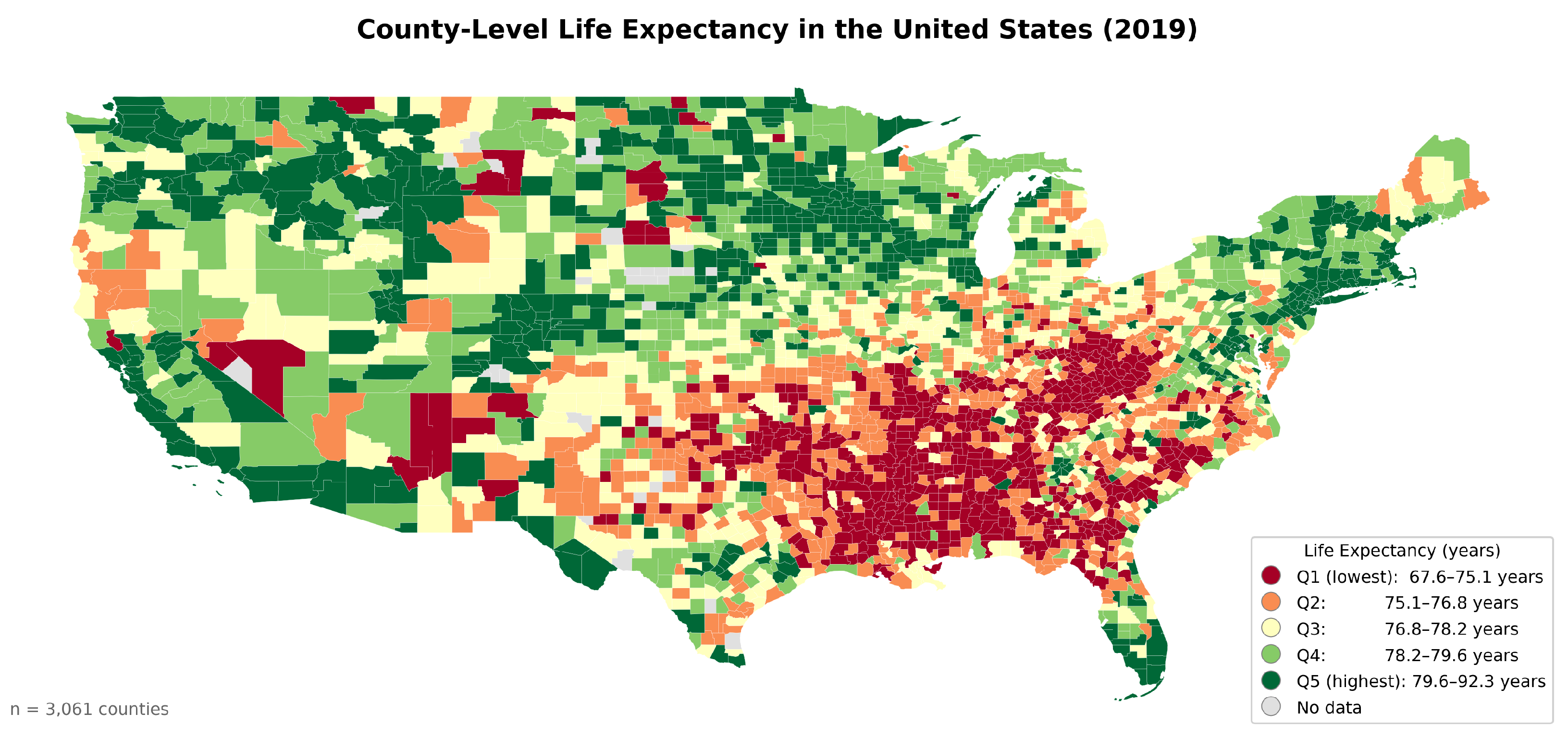
County-level life expectancy in the United States (2019). Values range from 67.6 to 92.3 years, with lower life expectancy concentrated in the South and Appalachia.
Figure 1.
County-level life expectancy in the United States (2019). Values range from 67.6 to 92.3 years, with lower life expectancy concentrated in the South and Appalachia.
Beyond socioeconomic factors, atmospheric and environmental exposures have also been demonstrated to influence life expectancy in a population. Air quality, in particular, has emerged as a significant determinant, with numerous studies linking elevated levels of environmental pollutants to increased morbidity and premature mortality [9,10]. Studies have linked fine particulate matter (PM2.5), nitrogen dioxide (NO2), and ground-level ozone (O3) exposure to an increased risk of mortality through respiratory and cardiovascular pathways [11,12,13]. Long-term exposure to PM2.5 has been associated with a shorter life expectancy, with studies estimating that a 10 g/m3 decrease in PM2.5 concentration corresponds to approximately 0.61 years of increased longevity [11]. Ozone exposure has similarly been linked to elevated mortality from respiratory causes, with risk increasing by up to 4% for each 10 ppb increment in average concentration [14]. In addition, formaldehyde exposure has been shown to increase the risks of leukemia and Hodgkin’s disease [15]. Livestock density has been proposed as a proxy for localized air quality degradation through greenhouse gas (GHG) emissions and spread of infectious zoonotic diseases such as avian influenza, Q-fever, and MERS [16]. Pig and cattle houses, in particular, have been shown to emit harmful pollutants like ammonia (), methane (), and nitrous oxide () [17,18]. Despite growing evidence of these environmental influences, to our knowledge, no prior study has integrated atmospheric, livestock, and socioeconomic data within a unified predictive framework at the county level.
Drawing on the external exposome framework, the totality of environmental exposures encountered throughout a lifetime [19], we develop an interpretable machine learning framework to model county-level life expectancy across the United States using an integrated dataset spanning socioeconomic, atmospheric, and livestock variables. We use data from the Institute for Health Metrics and Evaluation (IHME), the American Community Survey (ACS), the Copernicus Atmosphere Monitoring Service (CAMS), and livestock distribution datasets for the period 2012–2019 [1,16]. Our modeling approach employs XGBoost, a gradient boosting algorithm known for its ability to capture complex non-linear relationships and interactions among high-dimensional features [20], and utilizes SHAP values and permutation importance to identify the most influential determinants. Our analysis reveals that while traditional socioeconomic variables remain strong predictors, atmospheric variables such as formaldehyde exposure and wet-bulb temperature emerge as novel and significant determinants of life expectancy, providing new insights for targeted public health interventions.
Figure 2.
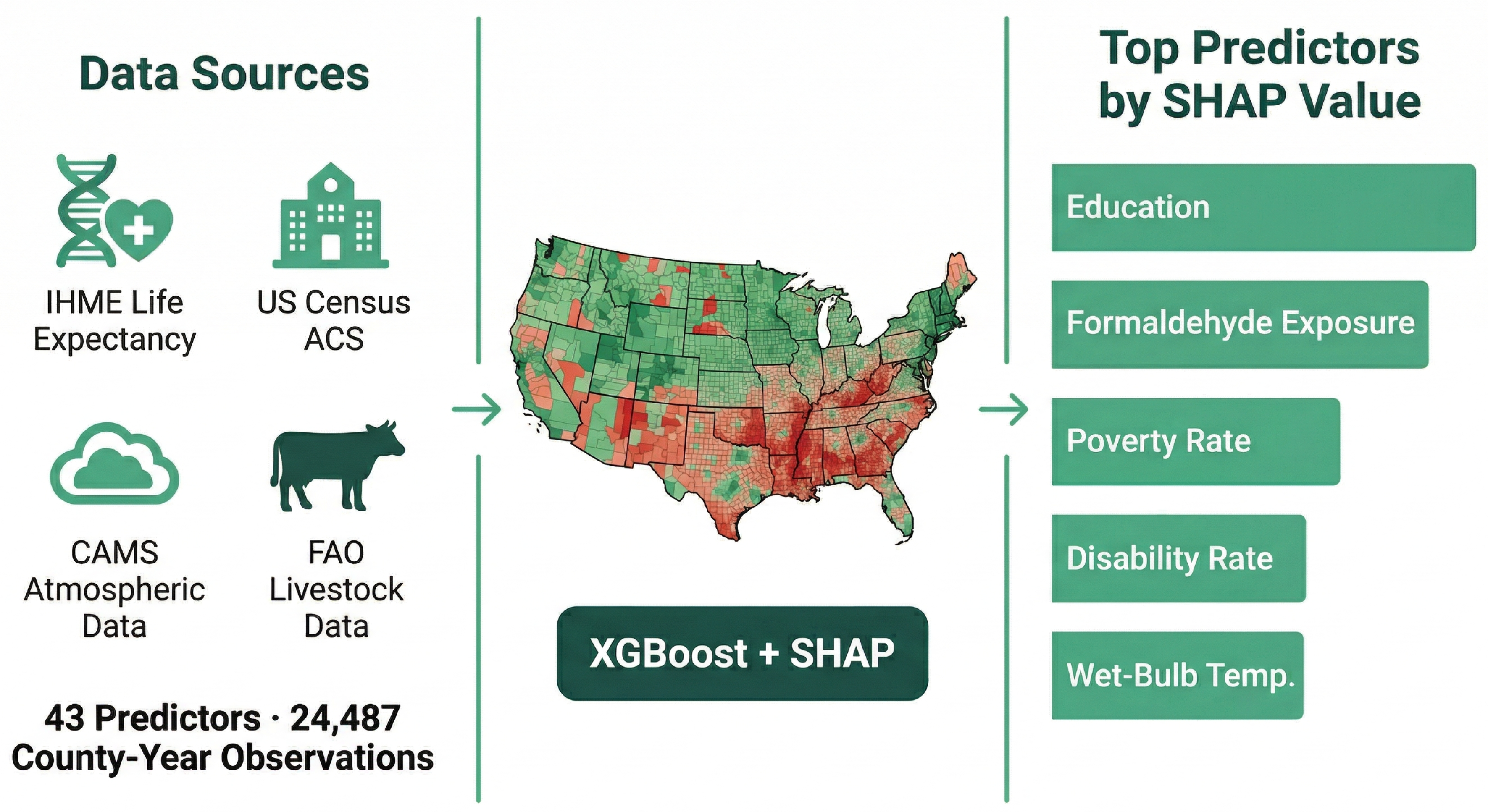
Study workflow. Four data sources are integrated into an XGBoost model with SHAP interpretability to identify the leading predictors of county-level life expectancy across the contiguous United States. Formaldehyde exposure ranked second among all 43 predictors, surpassed only by educational attainment.
Figure 2.
Study workflow. Four data sources are integrated into an XGBoost model with SHAP interpretability to identify the leading predictors of county-level life expectancy across the contiguous United States. Formaldehyde exposure ranked second among all 43 predictors, surpassed only by educational attainment.
2. Methodology
This study integrates county-level data from four primary sources to model life expectancy across the contiguous United States from 2012 to 2019. Life expectancy estimates were obtained from the Institute for Health Metrics and Evaluation (IHME) [21], while socioeconomic variables were drawn from the American Community Survey (ACS) 5-year estimates [22]. Atmospheric data, including pollutant concentrations and meteorological variables, were sourced from the Copernicus Atmosphere Monitoring Service (CAMS) and the European Centre for Medium-Range Weather Forecasts ERA5 reanalysis [23]. Livestock density data were obtained from Gilbert et al. [16]. Each of these datasets was preprocessed and combined, and the final integrated dataset was used to train an XGBoost model [20]. Model performance was evaluated using root mean square error (RMSE) and adjusted R², while feature importance was assessed through SHAP values and permutation importance. A brief description of the datasets that were used in this analysis is included below:
2.1. IHME Dataset
Life expectancy estimates were obtained from the Institute for Health Metrics and Evaluation (IHME), which provides annual county-level estimates of mean life expectancy at birth across the United States from 2000 to 2019 [21]. These estimates are derived from population and mortality data provided by the National Center for Health Statistics and represent stratified estimates by age group, race, and ethnicity [1]. For this study, we used life expectancy estimates for the total population, which includes all racial and ethnic groups, for individuals under 1 year of age, as this metric provides a standardized measure of overall population health at the county level. The IHME dataset covers all counties in the contiguous United States, enabling a comprehensive analysis of life expectancy disparities. Data from 2012 to 2019 were selected to align with the temporal coverage of the atmospheric and socioeconomic datasets.
2.2. ACS Dataset
Socioeconomic and demographic variables were obtained from the American Community Survey (ACS) 5-year estimates for 2012 to 2019 [22]. The 5-year estimates were selected over the 1-year estimates due to their greater statistical reliability for small geographic units such as counties, which is essential for county-level spatial modeling [24]. The 1-year estimates, while temporally more precise, only cover counties with populations of 65,000 or more and would have limited our analysis to non-rural areas [25].
We initially retrieved approximately 20 variables from the ACS using the U.S. Census Bureau API, including poverty rate, median household income, unemployment rate, educational attainment (percentage with a bachelor’s degree or higher), and racial composition. Racial composition was calculated as the proportion of each racial/ethnic group relative to the total county population. After removing highly correlated and redundant features during preprocessing, 10 variables were retained for the final model. These socioeconomic indicators were selected based on prior research linking income, education, and demographic structure to mortality and health outcomes [4,5]. The final retained variables are listed in the Appendix.
2.3. CAMS Dataset
Atmospheric and meteorological variables were obtained from the Copernicus Atmosphere Monitoring Service (CAMS) global reanalysis (EAC4) and the European Centre for Medium-Range Weather Forecasts (ECMWF) ERA5 reanalysis [23]. CAMS assimilates satellite observations including OMI for tropospheric composition, MODIS for aerosol optical depth, and GOME-2 for trace gases, combining remote sensing data with atmospheric modeling to provide spatially continuous estimates [23]. The CAMS EAC4 dataset provides gridded atmospheric composition data at 0.75° × 0.75° spatial resolution with 3-hourly temporal resolution, including air pollutants (PM2.5, O3, NO2, formaldehyde) at both surface level and total column, along with meteorological variables. ERA5 provided relative humidity data at 0.25° × 0.25° resolution. To match the county-level spatial resolution of the life expectancy data, the gridded raster data were spatially interpolated to county boundary points using multilinear interpolation, then averaged across boundary points for each county. Temporal aggregation was performed by calculating annual averages from the 3-hourly observations (approximately 2,960 time points per year). At the end, we had approximately 60 atmospheric features for 2012–2019, including pollutant concentrations, temperature, humidity, and wind velocity. Several atmospheric variables were derived as fraction-of-time (FoT) metrics, representing the fraction of time during which concentrations exceeded specific percentile thresholds. For example, formaldehyde exposure frequency (FoT Formaldehyde Above 75th Percentile) quantifies the proportion of time annually when formaldehyde concentrations exceeded the 75th percentile across all observations. A complete list of atmospheric variables is provided in Appendix.
2.4. Livestock Data
Livestock density data were obtained from the Food and Agriculture Organization (FAO) Gridded Livestock of the World (GLW) dataset, which provides species-specific density estimates (heads/km²) at approximately 10 km resolution for seven species: cattle, chicken, duck, goat, horse, pig, and sheep [16,26]. The gridded raster data were aggregated to county-level boundaries using area-weighted zonal statistics, with densities calculated only for agricultural land identified from the 2019 National Land Cover Database. Because GLW data were available only for discrete years (2010, 2015, 2020), annual values for 2012–2019 were generated through linear interpolation between these time points. This yielded seven livestock density features for each county–year observation, serving as proxies for agricultural intensity and associated environmental pollutants such as ammonia (), methane (), and nitrous oxide () [17].

Table 1.
Summary of data sources used in this study.
| Source | Description | Period | Resolution | N |
|---|---|---|---|---|
| IHME | Life expectancy at birth | 2012–2019 | County-level | 1 |
| ACS 5-year | Socioeconomic and demographic indicators | 2012–2019 | County-level | 10 |
| CAMS/ERA5 | Atmospheric pollutants and meteorological variables | 2012–2019 | County-level (from 0.75°/0.25° grids) | 26 |
| FAO GLW | Livestock density by species | 2012–2019 (interpolated) | County-level (from ∼10 km grids) | 7 |
| Total: 43 features | ||||
2.5. Data Processing
The four datasets were merged by county FIPS codes and year to create a unified panel dataset. Missing values, denoted either as NaN or as the sentinel value -666666666, were handled through listwise deletion to avoid introducing imputation bias and maintain internal consistency across features. To reduce multicollinearity among atmospheric variables, features with pairwise correlations exceeding 0.85 were identified through hierarchical clustering analysis, and the most interpretable feature from each correlated cluster was retained for modeling. Metadata columns such as County, State, and FIPS codes were retained for identification purposes but excluded from the feature matrix used for modeling. After preprocessing and cleaning, the final integrated dataset comprised 24,487 county-year observations spanning 2012–2019, with 43 predictor variables and 1 target variable (life expectancy). Because the datasets for 2012-2019 were stacked vertically and the same counties are repeated across multiple years, standard random splitting would have allowed observations from the same county to appear in both training and test sets, leading to data leakage and inflated performance metrics. To prevent this, we employed GroupShuffleSplit with county FIPS codes as the grouping variable, ensuring that all observations from a given county were assigned exclusively to either the training set (80%) or the test set (20%). This forces the model to predict the life expectancy of only those counties that it did not see during training.
2.6. Modeling Approach
The preprocessed dataset was used to train an XGBoost gradient boosting regressor, selected for its ability to capture complex non-linear relationships and feature interactions while incorporating L1 and L2 regularization to prevent overfitting [20]. Hyperparameter optimization was performed using Bayesian optimization via BayesSearchCV, which efficiently explores the hyperparameter space through probabilistic modeling rather than exhaustive grid search [27]. The search space included n_estimators (200–1500), max_depth (4–8), learning_rate (0.01–0.15), subsample (0.6–0.95), colsample_bytree (0.5–0.9), L1 regularization (reg_alpha, 0.01–5.0), L2 regularization (reg_lambda, 0.1–5.0), and min_child_weight (3–15). Bayesian optimization was configured with 30 iterations and 5-fold GroupKFold cross-validation, using R² as the optimization metric. GroupKFold ensures that during each cross-validation fold, all observations from a given county remain together, preventing the same county from appearing in both the training and validation portions of any fold. The best-performing hyperparameter configuration was selected and used to train the final model on the entire training set. The same optimization procedure was applied to reduced feature sets in the ablation analysis.
Model performance was evaluated using two complementary metrics: root mean squared error (RMSE) and adjusted R². RMSE was selected because it is expressed in the same units as the target variable (years), providing an intuitive measure of prediction error that directly quantifies the average deviation between predicted and actual life expectancy values. Adjusted R² was used to assess the proportion of variance explained by the model while penalizing model complexity, making it particularly suitable for high-dimensional datasets where standard R² can be inflated by the inclusion of numerous predictors. Both metrics were computed separately on training and test sets to evaluate model generalization and detect potential overfitting.
Table 2.
Optimal hyperparameters obtained through Bayesian optimization for the full 43-feature model.
Table 2.
Optimal hyperparameters obtained through Bayesian optimization for the full 43-feature model.
| Parameter | Optimal Value |
|---|---|
| n_estimators | 1457 |
| max_depth | 7 |
| learning_rate | 0.024 |
| subsample | 0.95 |
| colsample_bytree | 0.50 |
| reg_alpha | 0.08 |
| reg_lambda | 5.00 |
| min_child_weight | 15 |
2.7. Modeling Interpretability
To interpret the trained XGBoost model and identify the most influential predictors of life expectancy, we employed two complementary feature importance methods. Permutation importance was calculated by randomly shuffling each feature’s values in the test set and measuring the resulting degradation in model performance (RMSE), with greater performance drops indicating higher feature importance. SHAP (SHapley Additive exPlanations) values were computed using the TreeExplainer algorithm to quantify each feature’s contribution to individual predictions, providing both global importance rankings and directional effects [28]. Unlike permutation importance, SHAP values are grounded in cooperative game theory and account for feature interactions, offering more robust interpretability for correlated predictors [28]. To assess feature redundancy, we conducted an ablation study by systematically retraining the model with progressively reduced feature sets based on SHAP rankings (top 20, top 10, and top 5 features), evaluating the tradeoff between model complexity and predictive performance. Model calibration and prediction errors were assessed through residual analysis, examining the distribution and patterns of residuals (observed minus predicted values) across the range of predicted life expectancy values.
3. Results
3.1. Model Performance
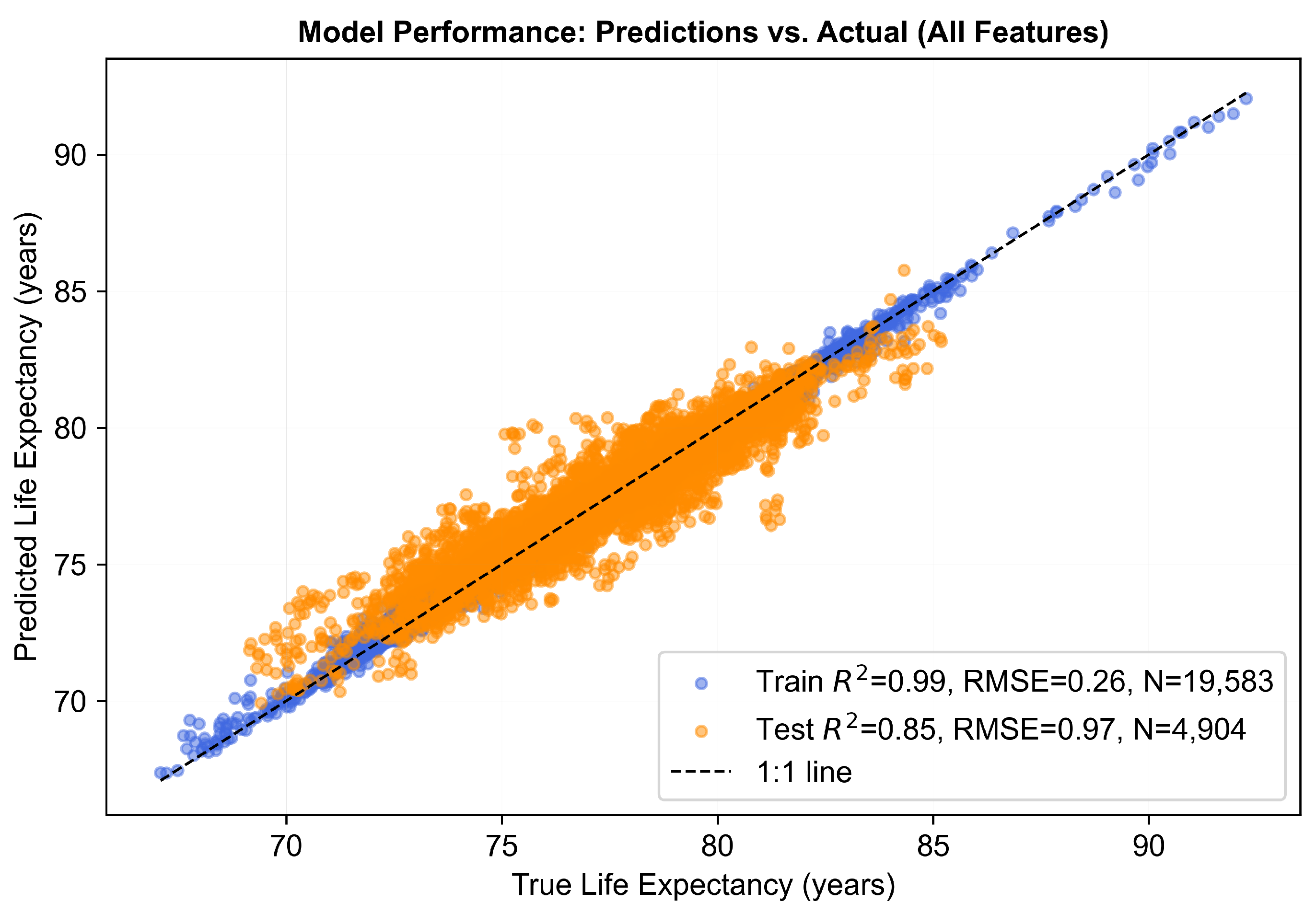
The XGBoost model trained on all 43 features achieved a test R² of 0.854 and test RMSE of 0.97 years, indicating strong predictive performance with an average prediction error of less than one year per county. Training performance showed R² = 0.989 and RMSE = 0.26 years. While the high training score indicates that the model has sufficient capacity to capture fine-grained variations within the training counties, the strong test performance (R² > 0.85) confirms that this does not represent simple memorization. The gap between training and test metrics is expected given the rigorous county-level cross-validation strategy (GroupShuffleSplit), which requires the model to generalize to entirely unseen geographic regions rather than merely interpolating between years for counties already observed during training. This test score effectively represents the model’s performance in a "future unseen county" scenario.
Figure 3.
Scatter plot of predicted versus actual life expectancy for training (blue) and test (orange) sets using the full 43-feature model. The diagonal dashed line represents perfect prediction.
Figure 3.
Scatter plot of predicted versus actual life expectancy for training (blue) and test (orange) sets using the full 43-feature model. The diagonal dashed line represents perfect prediction.
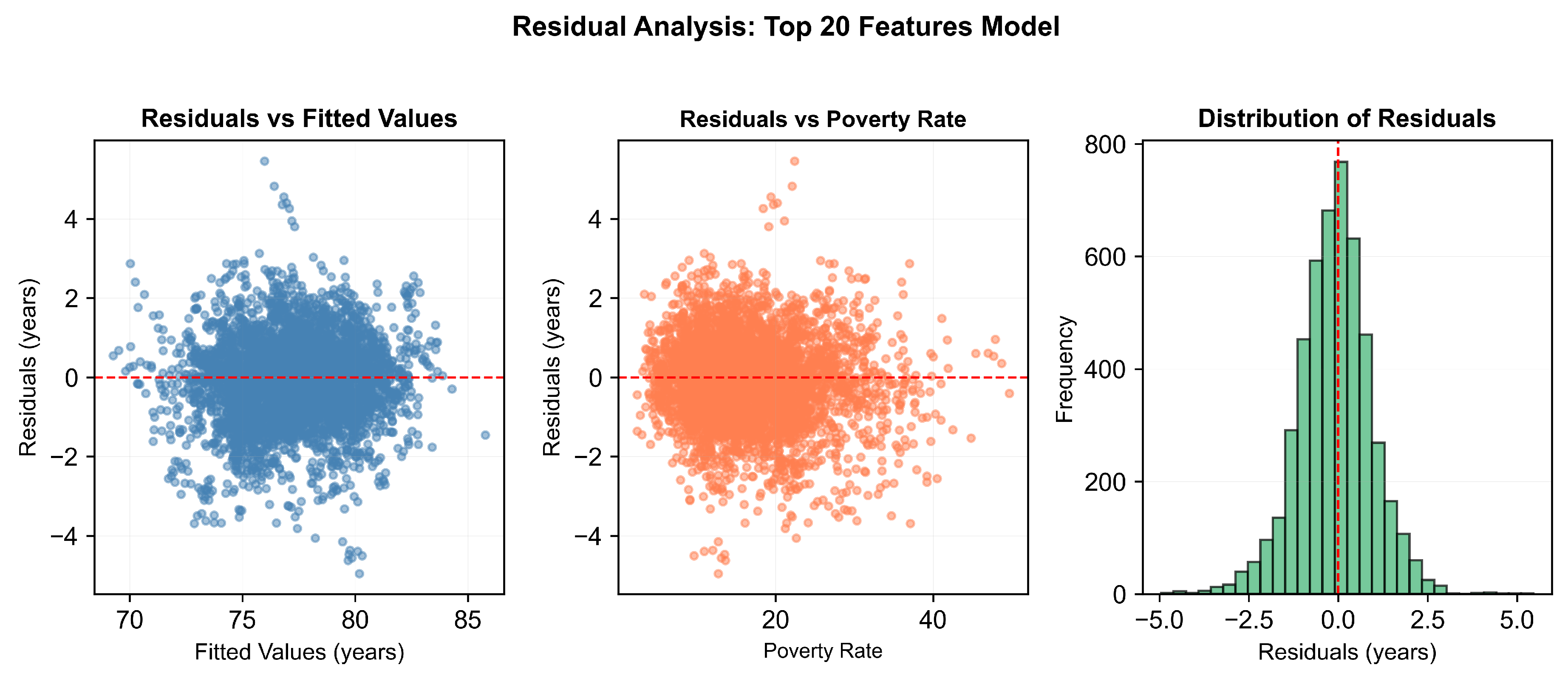
We validated the model’s reliability using residual plots (Figure 4). The errors appear random and show no obvious patterns across the range of predictions. Additionally, the distribution of errors forms a bell curve centered at zero, showing that the model is unbiased and its predictions are consistent.
Figure 4.
Residual diagnostics for the top 20 model. Left: residuals versus fitted values showing no systematic patterns. Center: residuals versus poverty rate confirming no predictor-related bias. Right: histogram of residuals demonstrating approximate normality.
Figure 4.
Residual diagnostics for the top 20 model. Left: residuals versus fitted values showing no systematic patterns. Center: residuals versus poverty rate confirming no predictor-related bias. Right: histogram of residuals demonstrating approximate normality.
3.2. Feature Importance Analysis
SHAP analysis of the 43-feature model identified educational attainment (Bachelor’s Degree or Higher) as the most important predictor, followed by the fraction of time in the year for which formaldehyde levels in the region exceeded the 75th percentile (FoT Formaldehyde Above 75th Percentile), poverty rate, disability rate, and wet-bulb temperature as the top five features (Figure 5). The complete ranking of the top 20 features included eight socioeconomic and demographic variables (education, poverty rate, disability rate, percentage of households with single mother families, Hispanic population percentage, White population percentage, total population, and percentage of households with no vehicle), eight atmospheric variables (formaldehyde, wet-bulb temperature, leaf area indices for high and low vegetation, hydrophilic black carbon aerosol mixing ratio, dust aerosol mixing ratio, propane, and nitric acid), and four livestock density measures (horse, pig, chicken, and cattle). Notably, formaldehyde exposure ranked second overall, placing it ahead of many social determinants of health and representing the highest-ranked atmospheric pollutant. Wet-bulb temperature ranked fifth, making it the second atmospheric variable in the top five predictors.
Figure 5.
SHAP summary plot (beeswarm) showing feature importance and directional effects for the top 20 predictors in the 43-feature model. Each point represents a single county-year observation, with color indicating feature value (red = high, blue = low). Higher educational attainment and lower poverty rates are associated with increased life expectancy, while higher formaldehyde exposure is associated with decreased life expectancy.
Figure 5.
SHAP summary plot (beeswarm) showing feature importance and directional effects for the top 20 predictors in the 43-feature model. Each point represents a single county-year observation, with color indicating feature value (red = high, blue = low). Higher educational attainment and lower poverty rates are associated with increased life expectancy, while higher formaldehyde exposure is associated with decreased life expectancy.
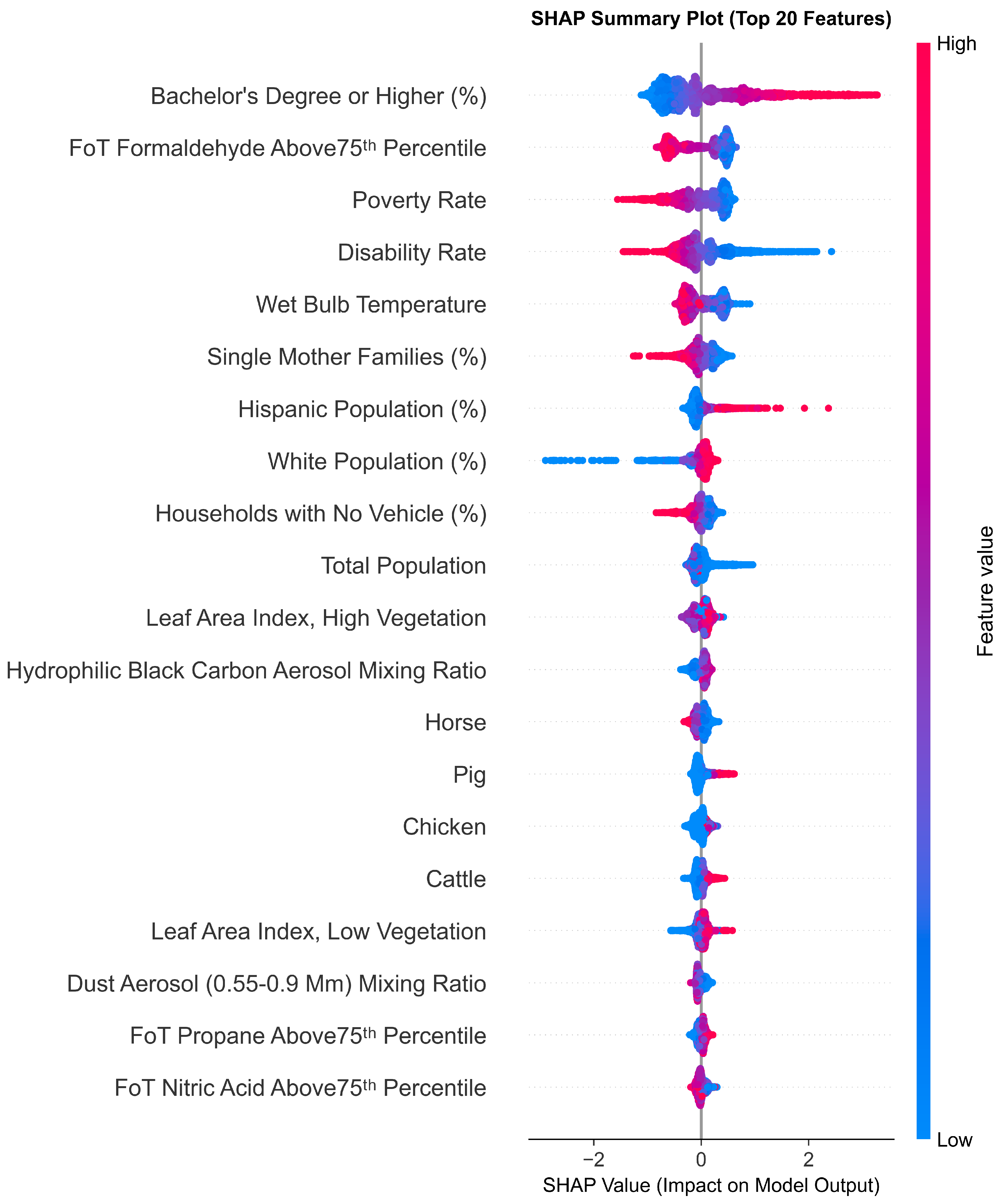
Socioeconomic predictors were found to be the most prominent in the importance rankings, with educational attainment showing the highest SHAP importance. The beeswarm plot (Figure 5) revealed clear directional effects: higher percentages of bachelor’s degree holders (red points) consistently pushed predictions toward higher life expectancy (positive SHAP values on the right), while lower educational attainment (blue points) was associated with lower predicted life expectancy (negative SHAP values on the left). Poverty rate showed an inverse relationship, with higher poverty rates (red points) driving predictions toward lower life expectancy (negative SHAP values). Disability rate similarly demonstrated negative associations, with higher disability rates corresponding to lower life expectancy predictions. These patterns aligned with established literature linking socioeconomic disadvantage to adverse health outcomes [4,5].
Atmospheric and environmental variables appeared prominently among top predictors, with two features in the top five. Formaldehyde exposure ranked second overall, showing predominantly negative SHAP values for high exposure (red points on the left side of the beeswarm plot), indicating that counties with frequent formaldehyde levels exceeding the 75th percentile experienced lower predicted life expectancy. Wet-bulb temperature ranked fifth, showing predominantly negative SHAP values for higher temperatures (red points on the left), suggesting that heat stress conditions negatively impact life expectancy predictions. Additional atmospheric variables in the top 20 included leaf area indices (both high and low vegetation), hydrophilic black carbon aerosol mixing ratio, dust aerosol mixing ratio, propane exposure frequency, and nitric acid exposure frequency, suggesting that environmental factors contribute meaningfully to life expectancy variation beyond traditional socioeconomic determinants. Livestock density variables (horse, pig, chicken, and cattle) appeared among secondary predictors, ranking 13th through 16th.
3.3. Feature Ablation Study
To identify which features were redundant, we retrained the XGBoost model using progressively reduced feature sets based on SHAP importance rankings from the full 43-feature model. Three reduced models were trained using the top 20, top 10, and top 5 features, with hyperparameters recalculated through Bayesian optimization for each configuration. Performance metrics across all models are shown in Table 3 and Figure 6.
Figure 6.
Ablation study showing model performance (Test R² and RMSE) as a function of the number of features. Performance declines gradually from 43 to 20 features, indicating some redundancy among lower-ranked predictors. Performance declines more progressively below 20 features, with notable degradation at 5 features.
Figure 6.
Ablation study showing model performance (Test R² and RMSE) as a function of the number of features. Performance declines gradually from 43 to 20 features, indicating some redundancy among lower-ranked predictors. Performance declines more progressively below 20 features, with notable degradation at 5 features.
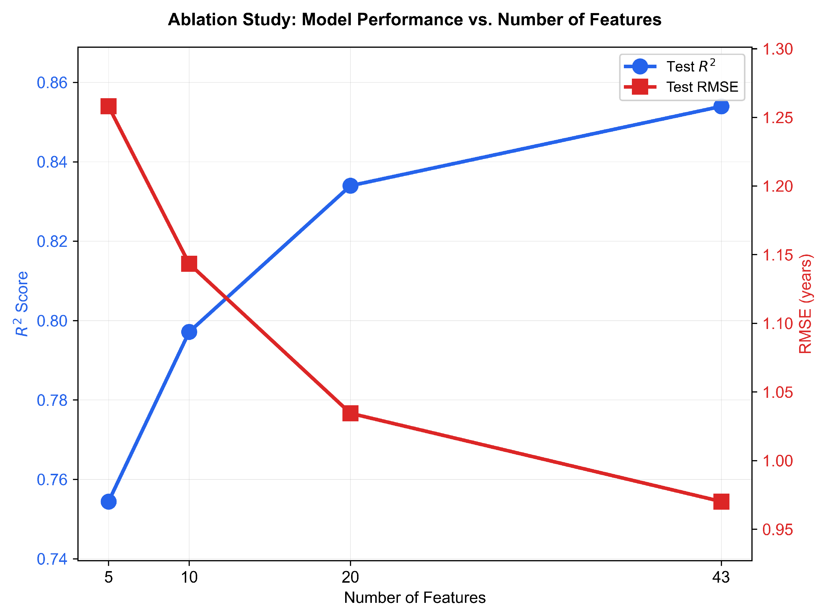
The top 20 model achieved strong performance (R² = 0.834, RMSE = 1.03 years), only slightly below the full 43-feature model (R² = 0.854, RMSE = 0.97 years), demonstrating that the 23 lowest-ranked features contributed minimal predictive information. The top 10 model maintained reasonably strong performance (R² = 0.797, RMSE = 1.14 years), representing a modest degradation of 0.037 in R² compared to the top 20 model. Performance declined more substantially when reducing to 5 features (R² = 0.754, RMSE = 1.26 years), indicating that the information threshold lies between 5 and 10 features. The ablation curve (Figure 6) illustrates this pattern clearly, with R² declining gradually from 43 to 20 features and more progressively below 20 features.
Feature importance rankings remained consistent across reduced models. In the full 43-feature model, educational attainment ranked first, formaldehyde exposure second, and poverty rate third. In the top 20 model, permutation importance analysis revealed disability rate in second position, with formaldehyde exposure third (Figure 7). In the top 10 and top 5 models, formaldehyde exposure remained consistently among the top five features. The consistent presence of formaldehyde exposure among top predictors across all configurations suggests it captures unique health-relevant information that remains important even in highly reduced feature sets. This trend was corroborated by both SHAP rankings and permutation importance, with both methods independently identifying formaldehyde exposure as a leading predictor.
Figure 7.
Permutation importance for the top 20 model. The ranking shows educational attainment first, disability rate second, and formaldehyde exposure third, with poverty rate fourth. This partially differs from SHAP rankings, where formaldehyde ranked second, highlighting that different interpretability methods capture complementary aspects of feature importance.
Figure 7.
Permutation importance for the top 20 model. The ranking shows educational attainment first, disability rate second, and formaldehyde exposure third, with poverty rate fourth. This partially differs from SHAP rankings, where formaldehyde ranked second, highlighting that different interpretability methods capture complementary aspects of feature importance.
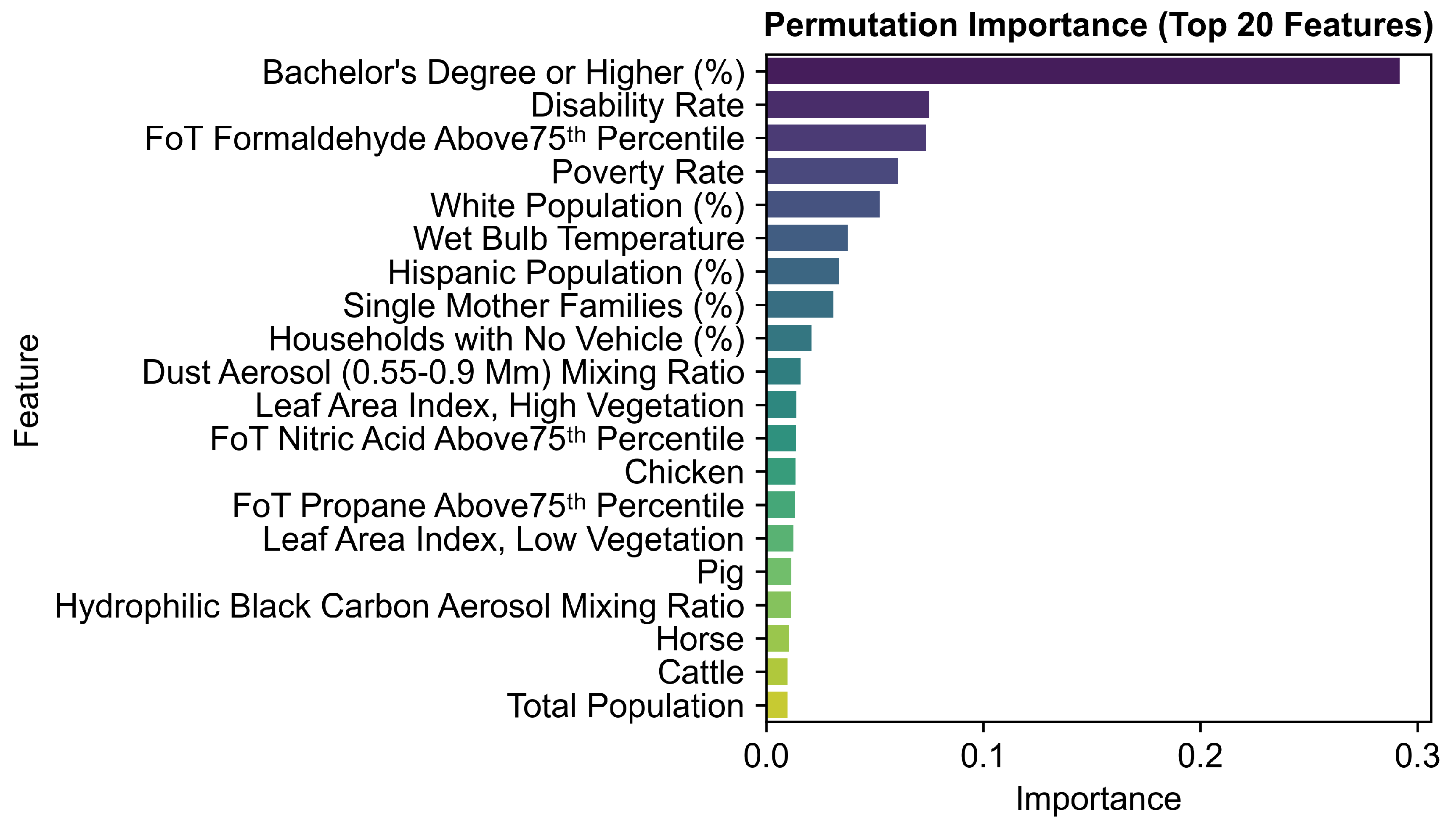
The strong performance of the top 20 model compared to the full model demonstrates substantial redundancy among lower-ranked features. A model using 20 carefully selected features achieves nearly the same predictive accuracy as one using all 43 features (R² of 0.834 vs 0.854), while improving interpretability and reducing computational requirements. The consistency of formaldehyde’s prominence across all model configurations, ranking second in SHAP importance and third in permutation importance, strengthens confidence in its role as a meaningful predictor of county-level life expectancy beyond conventional socioeconomic determinants.
Table 3.
Model performance metrics across feature ablation study. The top 20 model achieves nearly equivalent performance to the full model with less than half as many features.
Table 3.
Model performance metrics across feature ablation study. The top 20 model achieves nearly equivalent performance to the full model with less than half as many features.
| Feature Set | N Features | Train R² | Test R² | Train RMSE | Test RMSE | Test MAE |
|---|---|---|---|---|---|---|
| All Features | 43 | 0.989 | 0.854 | 0.26 | 0.97 | 0.73 |
| Top 20 | 20 | 0.940 | 0.834 | 0.62 | 1.03 | 0.79 |
| Top 10 | 10 | 0.949 | 0.797 | 0.57 | 1.14 | 0.86 |
| Top 5 | 5 | 0.806 | 0.754 | 1.12 | 1.26 | 0.96 |
4. Discussion
4.1. Formaldehyde: An Underappreciated Environmental Determinant
The emergence of formaldehyde exposure as an important predictor of life expectancy represents a novel finding with important implications for environmental health. Formaldehyde is a ubiquitous volatile organic compound (VOC) with indoor sources (building materials, pressed wood products, household furniture, combustion appliances) and outdoor sources (vehicle emissions, industrial processes, photochemical reactions in the atmosphere) [29,30]. Despite widespread population exposure, formaldehyde has received considerably less attention in life expectancy modeling compared to more extensively studied air pollutants such as fine particulate matter (PM2.5) and ozone.
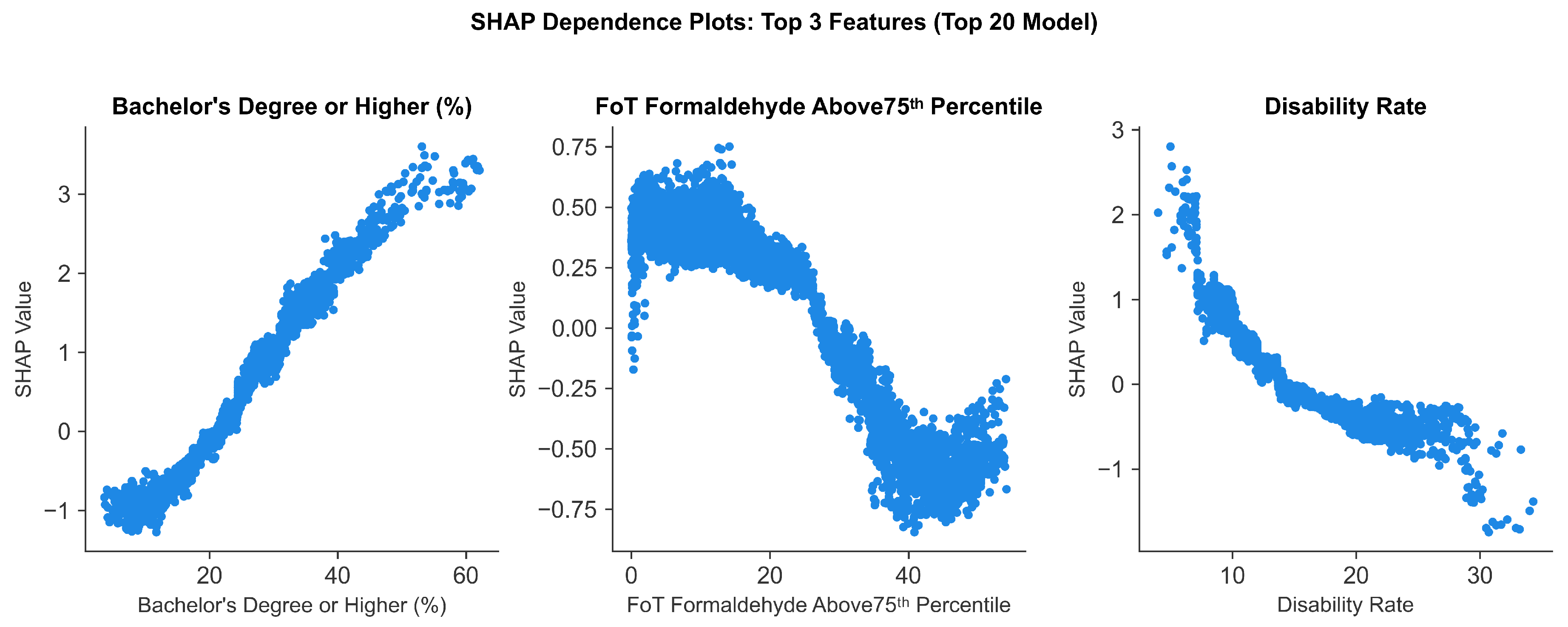
Formaldehyde is classified by the International Agency for Research on Cancer (IARC) as a Group 1 human carcinogen, with sufficient evidence linking exposure to nasopharyngeal cancer and leukemia [31]. It is also classified as a carcinogen (Category 1B) and mutagen (Category 2) by the European Commission [29]. Beyond carcinogenic effects, studies have shown that short-term exposure to low formaldehyde concentrations significantly increases mortality risks from non-accidental, circulatory, and respiratory diseases [32]. Formaldehyde exposure can also induce cardiovascular diseases including arrhythmia, myocardial infarction, heart failure, and atherosclerosis [33]. The biological mechanisms underlying these health effects include oxidative stress, systemic inflammation, DNA damage, and immunological dysregulation [34,35]. Given these well-documented health hazards, formaldehyde’s prominence as a predictor of county-level life expectancy is both biologically plausible and epidemiologically significant. The SHAP dependence plot (Figure 8) further reveals a non-linear threshold effect: SHAP values remain positive when formaldehyde exceeds the 75th percentile less than approximately 30% of the time but decline sharply beyond this point. This pattern is consistent with dose-response relationships in which biological detoxification mechanisms can manage intermittent exposure but become overwhelmed under sustained or chronic conditions [34].
Current air quality monitoring prioritizes criteria pollutants (ozone, particulate matter, carbon monoxide, sulfur dioxide, nitrogen dioxide, and lead), leaving formaldehyde largely unmonitored [36] despite classification as a Hazardous Air Pollutant (HAP) under Clean Air Act Section 112 [37]. Ground-level formaldehyde observations remain particularly sparse [38], limiting the ability to assess population exposure and health risks comprehensively. Satellite remote sensing provides a solution to this monitoring gap, with instruments such as OMI and TROPOMI enabling spatially continuous formaldehyde column observations at resolutions as fine as 3.5×5.5 km, complementing sparse ground-based networks [39]. While our observational study cannot establish causality, the prominence and consistency of formaldehyde in our models combined with established biological mechanisms linking formaldehyde exposure to adverse health outcomes, provide strong motivation for future epidemiological research employing enhanced exposure assessment and causal inference designs.
4.2. Socioeconomic Factors and Climate-Related Predictors
Percentage of population with a bachelor’s degree or higher (educational attainment) emerged as the strongest predictor across all model configurations, confirming extensive literature documenting the role of socioeconomic determinants in predicting health outcomes [4,40]. Notably, formaldehyde exposure ranked second in the full 43-feature model, surpassing poverty rate and other traditional socioeconomic indicators. Counties with higher educational attainment and lower poverty rates consistently showed higher predicted life expectancy across all models. The prominence of formaldehyde exposure, which ranked higher than poverty rate in the optimal model, indicates that environmental air quality operates as a distinct measure that influences population health, rather than simply serving as a proxy for socioeconomic disadvantage. This finding suggests that addressing health disparities requires integrated strategies that targets both socioeconomic determinants and environmental exposures.
Figure 8.
SHAP dependence plots for the top three predictors. The y-axis shows the feature’s specific impact on life expectancy (in years). (Left) Education shows a positive trend that flattens at higher percentages. (Center) Formaldehyde exposure shows a sharp drop in life expectancy once it exceeds the 75th percentile more than approximately 30% of the time. (Right) Poverty rate shows a consistent negative trend.
Figure 8.
SHAP dependence plots for the top three predictors. The y-axis shows the feature’s specific impact on life expectancy (in years). (Left) Education shows a positive trend that flattens at higher percentages. (Center) Formaldehyde exposure shows a sharp drop in life expectancy once it exceeds the 75th percentile more than approximately 30% of the time. (Right) Poverty rate shows a consistent negative trend.
Wet-bulb temperature, which consistently ranked among the top five features in our models, was another key variable that could offer valuable insights into how climate can affect life expectancy. Unlike dry bulb temperature, wet-bulb temperature accounts for both heat and humidity, providing a more physiologically relevant indicator of heat stress and the human body’s ability to thermoregulate through evaporation [41]. Lately, regions around the world are experiencing critical wet bulb temperatures that frequently exceed thresholds beyond which human thermoregulation becomes impaired [41,42]. In particular, a wet-bulb temperature of approximately 35°C represents a theoretical upper limit for sustained human survival, beyond which the body can no longer dissipate metabolic heat through perspiration [42,43]. Studies have documented associations between extreme wet-bulb temperatures and increased mortality rates [44,45], suggesting that combined heat and humidity metrics capture physiologically relevant exposure patterns better than temperature measurements alone. The prominence of wet-bulb temperature in our predictive models aligns with this physiological evidence and indicates that heat stress, when measured through this combined metric, correlates with population-level life expectancy variation across US counties.
4.3. Limitations and Future Directions
This study has several limitations. The observational design documents associations between formaldehyde exposure and life expectancy but cannot establish causality. County-level aggregation introduces ecological fallacy risk, as population-level associations may not reflect individual-level relationships. Atmospheric formaldehyde concentrations were derived from CAMS/ERA5 reanalysis models rather than ground-based monitors, introducing measurement uncertainty. Furthermore, the spatial resolution of the CAMS data ( 80 km) is coarser than many US counties, particularly in the eastern states, meaning that multiple counties may share identical atmospheric values; this spatial smoothing likely attenuates localized exposure gradients and may underestimate the true strength of atmospheric associations. Additionally, this study does not include county-level behavioral risk factors such as smoking prevalence, obesity rates, and physical inactivity, which are established determinants of life expectancy. However, these behavioral factors are strongly socially patterned, and educational attainment and poverty, both of which are included in our model, are well-established predictors of population health behaviors at the county level [46], suggesting that our socioeconomic variables partially capture behavioral variation. Future work could investigate whether atmospheric predictors retain their significance after directly adjusting for behavioral covariates. The analysis covers US counties during 2012–2019; generalization to other countries or time periods remains untested. Future research employing causal inference designs, individual-level exposure assessments, and mechanistic investigations is therefore needed to determine whether formaldehyde exposure causally impacts mortality. Expansion of ground-based formaldehyde monitoring networks, particularly in regions with high predicted exposure, would improve exposure assessment and enable validation of satellite-derived estimates.
5. Conclusions
This study demonstrates that an external exposome approach integrating atmospheric, socioeconomic, and environmental data with machine learning can identify novel determinants of population health. Formaldehyde exposure emerged as a robust predictor of county-level life expectancy, ranking among the top three features across multiple model configurations and surpassing several traditional socioeconomic indicators. Combined with wet-bulb temperature as an indicator of heat-humidity stress, our findings suggest that atmospheric exposures warrant greater attention in public health surveillance and intervention strategies. As these findings represent population-level associations at the county scale, future research should incorporate individual-level exposure and outcome data to establish causal pathways.
Author Contributions
Conceptualization, S.S. and D.J.L.; methodology, S.S.; software, S.S.; validation, S.S.; formal analysis, S.S.; investigation, S.S.; resources, D.J.L.; data curation, S.S., S.R. and F.A.; writing—original draft preparation, S.S.; writing—review and editing, D.J.L.; visualization, S.S.; supervision, D.J.L.; project administration, D.J.L. All authors have read and agreed to the published version of the manuscript.
Funding
This research received no external funding.
Data Availability Statement
Code and processed data are available at https://github.com/samyakshrestha/predicting-life-expectancy. Raw data sources are publicly available from the Institute for Health Metrics and Evaluation (IHME), U.S. Census Bureau American Community Survey, Copernicus Atmosphere Monitoring Service (CAMS), European Centre for Medium-Range Weather Forecasts (ECMWF) ERA5, and Food and Agriculture Organization (FAO) Gridded Livestock of the World as cited in this manuscript.
Acknowledgments
The authors used Claude (Anthropic) and Gemini (Google) to assist with manuscript writing, coding, and graphical abstract generation. All outputs were reviewed, validated, and edited by the authors, who take full responsibility for the content.
Conflicts of Interest
The authors declare no conflict of interest.
Appendix A. Variable Descriptions
Table A1 presents the complete list of 43 predictor variables used in the final models. From an initial set of approximately 100 atmospheric features extracted from CAMS and ERA5, we retained 26 after removing redundant physical measurements (e.g., duplicate aerosol optical depth wavelengths, total column gases) and highly correlated variables (r > 0.85) through hierarchical clustering analysis, as described in Section 2.5. The final feature set comprises 10 socioeconomic and demographic variables from the American Community Survey, 26 atmospheric and meteorological variables from CAMS/ERA5, and 7 livestock density variables from the FAO Gridded Livestock of the World dataset.
Note on Fraction-of-Time (FoT) Metrics: FoT variables represent the percentage of time during a year when pollutant concentrations exceeded the 75th percentile threshold calculated across all county-year observations in the dataset. For example, “FoT Formaldehyde Above 75th Percentile” quantifies the proportion of 3-hourly observations in a given year when formaldehyde concentrations in a county exceeded the 75th percentile value computed from the entire 2012–2019 dataset.
Table A1.
Complete list of 43 predictor variables used in the XGBoost models, organized by data source.
Table A1.
Complete list of 43 predictor variables used in the XGBoost models, organized by data source.
| Variable Name | Description | Unit |
|---|---|---|
| Socioeconomic and Demographic (N=10) | ||
| Poverty Rate | Population below poverty line | % |
| Bachelor’s Degree or Higher (%) | Percentage with bachelor’s degree or higher | % |
| Disability Rate | Population with disability | % |
| Total Population | County population | count |
| Unemployment Rate | Labor force unemployed | % |
| White Population (%) | White population percentage | % |
| Hispanic Population (%) | Hispanic/Latino population percentage | % |
| Black Population (%) | Black/African American population percentage | % |
| Households with No Vehicle (%) | Households without vehicle | % |
| Single Mother Families (%) | Families headed by single mothers | % |
| Atmospheric and Meteorological (N=26) | ||
| Land-sea Mask | Land-sea boundary indicator | - |
| Mean Sea Level Pressure | Mean sea level pressure | Pa |
| Dust Aerosol (0.55–0.9 m) Mixing Ratio | Fine dust aerosol mixing ratio | kg/kg |
| Dust Aerosol (0.9–20 m) Mixing Ratio | Coarse dust aerosol mixing ratio | kg/kg |
| Hydrophilic Black Carbon Aerosol Mixing Ratio | Hydrophilic black carbon mixing ratio | kg/kg |
| Hydrophobic Black Carbon Aerosol Mixing Ratio | Hydrophobic black carbon mixing ratio | kg/kg |
| Hydrophobic Organic Matter Aerosol Mixing Ratio | Hydrophobic organic matter mixing ratio | kg/kg |
| Sea Salt Aerosol (0.5–5 m) Mixing Ratio | Fine sea salt mixing ratio | kg/kg |
| Sea Salt Aerosol (5–20 m) Mixing Ratio | Coarse sea salt mixing ratio | kg/kg |
| Sulphate Aerosol Mixing Ratio | Sulphate aerosol mixing ratio | kg/kg |
| Leaf Area Index, High Vegetation | High vegetation leaf area index | m2/m2 |
| Leaf Area Index, Low Vegetation | Low vegetation leaf area index | m2/m2 |
| Snow Depth | Mean snow depth | m |
| 10m Wind Speed | Wind speed at 10m height | m/s |
| Wet Bulb Temperature | Mean wet bulb temperature | K |
| FoT Carbonmonoxide Above75th Percentile | Time CO > 75th percentile | % |
| FoT Ethane Above75th Percentile | Time ethane > 75th percentile | % |
| FoT Formaldehyde Above75th Percentile | Time formaldehyde > 75th percentile | % |
| FoT Hydroxyl Radical Above75th Percentile | Time OH > 75th percentile | % |
| FoT Nitric Acid Above75th Percentile | Time HNO3 > 75th percentile | % |
| FoT Nitrogen Dioxide Above75th Percentile | Time NO2 > 75th percentile | % |
| FoT Nitrogen Monoxide Above75th Percentile | Time NO > 75th percentile | % |
| FoT Ozone Above75th Percentile | Time O3 > 75th percentile | % |
| FoT PM2.5 Above75th Percentile | Time PM2.5 > 75th percentile | % |
| FoT Propane Above75th Percentile | Time propane > 75th percentile | % |
| FoT Sulphur Dioxide Above75th Percentile | Time SO2 > 75th percentile | % |
| Livestock Density (N=7) | ||
| Cattle | Cattle density | heads/km2 |
| Chicken | Chicken density | heads/km2 |
| Duck | Duck density | heads/km2 |
| Goat | Goat density | heads/km2 |
| Horse | Horse density | heads/km2 |
| Pig | Pig density | heads/km2 |
| Sheep | Sheep density | heads/km2 |
References
- Dwyer-Lindgren, L.; Bertozzi-Villa, A.; Stubbs, R.W.; et al. Inequalities in life expectancy among US counties, 1980 to 2014: temporal trends and key drivers. JAMA Internal Medicine 2017, 177, 1003–1011. [Google Scholar] [CrossRef]
- Murray, C.J.; et al. The state of US health, 1990–2010: burden of diseases, injuries, and risk factors. JAMA 2013, 310, 591–608. [Google Scholar] [CrossRef]
- Ho, J.Y. Causes of America’s Lagging Life Expectancy: An International Comparative Perspective. The Journals of Gerontology: Series B, Psychological Sciences and Social Sciences 2022, 77, S117–S126. [Google Scholar] [CrossRef]
- Chetty, R.; Stepner, M.; Abraham, S.; Lin, S.; Scuderi, B.; Turner, N.; Bergeron, A.; Cutler, D.M. The Association Between Income and Life Expectancy in the United States, 2001–2014. JAMA 2016, 315, 1750–1766. [Google Scholar] [CrossRef] [PubMed] [PubMed Central]
- Singh, G.K.; Lee, H. Marked Disparities in Life Expectancy by Education, Poverty Level, Occupation, and Housing Tenure in the United States, 1997–2014. Int. J. MCH AIDS 2021, 10, 7–18. [Google Scholar] [CrossRef]
- Liu, L.; Wen, W.; Shrubsole, M.J.; Lipworth, L.E.; Mumma, M.T.; Ackerly, B.A.; Shu, X.O.; Blot, W.J.; Zheng, W. Impacts of Poverty and Lifestyles on Mortality: A Cohort Study in Predominantly Low-Income Americans. American Journal of Preventive Medicine 2024, 67, 15–23. [Google Scholar] [CrossRef]
- Raghupathi, V.; Raghupathi, W. The influence of education on health: an empirical assessment of OECD countries for the period 1995–2015. Archives of Public Health 2020, 78, 20. [Google Scholar] [CrossRef] [PubMed]
- Zajacova, A.; Lawrence, E.M. The relationship between education and health: reducing disparities through a contextual approach. Annual Review of Public Health Final edited form published January 12. 2018, 39, 273–289. [Google Scholar] [CrossRef] [PubMed]
- Kelly, F.J.; Fussell, J.C. Air pollution and public health: emerging hazards and improved understanding of risk. Environmental Geochemistry and Health 2015, 37, 631–649. [Google Scholar] [CrossRef]
- Manisalidis, I.; Stavropoulou, E.; Stavropoulos, A.; Bezirtzoglou, E. Environmental and Health Impacts of Air Pollution: A Review. Frontiers in Public Health 2020, 8, 14. [Google Scholar] [CrossRef] [PubMed]
- Pope, C.A., III; Ezzati, M.; Dockery, D.W. Fine-Particulate Air Pollution and Life Expectancy in the United States. New England Journal of Medicine 2009, 360, 376–386. [Google Scholar] [CrossRef]
- Di, Q.; Wang, Y.; Zanobetti, A.; Wang, Y.; Koutrakis, P.; Choirat, C.; Dominici, F.; Schwartz, J.D. Air Pollution and Mortality in the Medicare Population. New England Journal of Medicine 2017, 376, 2513–2522. [Google Scholar] [CrossRef]
- Crouse, D.L.; Peters, P.A.; Hystad, P.; Brook, J.R.; van Donkelaar, A.; Martin, R.V.; Villeneuve, P.J.; Jerrett, M.; Goldberg, M.S.; III, C.A.P.; et al. Ambient PM2.5, O3, and NO2 exposures and associations with mortality over 16 years of follow-up in the Canadian Census Health and Environment Cohort (CanCHEC). Environmental Health Perspectives 2015, 123, 1180–1186. [Google Scholar] [CrossRef]
- Jerrett, M.; Burnett, R.T.; III, C.A.P.; Ito, K.; Thurston, G.; Krewski, D.; Shi, Y.; Calle, E.; Thun, M. Long-term ozone exposure and mortality. The New England Journal of Medicine 2009, 360, 1085–1095. [Google Scholar] [CrossRef] [PubMed]
- Beane Freeman, L.E.; Blair, A.; Lubin, J.; Stewart, P.A.; Hein, M.J.; Rothman, N.; Alavanja, M.C.R.; et al. Mortality From Lymphohematopoietic Malignancies Among Workers in Formaldehyde Industries: The National Cancer Institute Cohort. Journal of the National Cancer Institute 2009, 101, 751–761. [Google Scholar] [CrossRef] [PubMed]
- Gilbert, M.; Nicolas, G.; Cinardi, G.; Van Boeckel, T.P.; Vanwambeke, S.O.; Wint, G.W.; Robinson, T.P. Global distribution data for cattle, buffaloes, horses, sheep, goats, pigs, chickens and ducks in 2010. Scientific Data 2018, 5, 1–12. [Google Scholar] [CrossRef]
- Anestis, V.; Umar, W.; Dragoni, F.; van der Weerden, T.J.; Hassouna, M.; Noble, A.; Bartzanas, T.; Amon, B. Mitigation of greenhouse gas and ammonia emissions due to livestock housing management practices: Analysis of the DATAMAN database. Biosystems Engineering 2025, 258, 104260. [Google Scholar] [CrossRef]
- Rigolot, C.; Espagnol, S.; Robin, P.; Hassouna, M.; Béline, F.; Paillat, J.M.; Dourmad, J.Y. Modelling of manure production by pigs and NH3, N2O and CH4 emissions. Part II: effect of animal housing, manure storage and treatment practices. Animal 2010, 4, 1413–1424. [Google Scholar] [CrossRef] [PubMed]
- Wild, C.P. The exposome: from concept to utility. International Journal of Epidemiology 2012, 41, 24–32. [Google Scholar] [CrossRef]
- Chen, T.; Guestrin, C. XGBoost: A scalable tree boosting system. In Proceedings of the Proceedings of the 22nd ACM SIGKDD international conference on knowledge discovery and data mining. ACM, 2016; pp. 785–794. [Google Scholar]
- for Health Metrics, I.; (IHME), E. United States Mortality Rates and Life Expectancy by County, Race, and Ethnicity 2000–2019. Global Health Data Exchange (GHDx);GHDx record “United States Life Expectancy by County, Race & Ethnicity 2000-2019”.
- U.S. Census Bureau. American Community Survey 5-Year Data (2009–2023). 2024. Available online: https://www.census.gov/data/developers/data-sets/acs-5year.html.
- Inness, A.; Ades, M.; Agustí-Panareda, A.; Barré, J.; Benedictow, A.; Blechschmidt, A.M.; Dominguez, J.J.; Engelen, R.; Eskes, H.; Flemming, J.; et al. The CAMS reanalysis of atmospheric composition. Atmospheric Chemistry and Physics 2019, 19, 3515–3556. [Google Scholar] [CrossRef]
- Bureau, U.S.C. American Community Survey (ACS) 5-Year Estimates. 2023. Available online: https://www.census.gov/programs-surveys/acs/technical-documentation.html https://www.census.gov/data/developers/data-sets/acs-5year.html.
- U.S. Census Bureau. American Community Survey 1-Year Data (2005–2024). 2025. Page last revised August 28, 2025. Available online: https://www.census.gov/data/developers/data-sets/acs-1year.html.
- Wint, G.R.W.; Robinson, T.P. Gridded Livestock of the World, 2007; Accessed; Food and Agriculture Organization of the United Nations: Rome, Italy, 2007. [Google Scholar]
- Wild Tree Tech.; Google Brain.; University of Liège.; Saarland University. scikit-optimize: Sequential model-based optimization in Python. 2020. Available online: https://scikit-optimize.github.io/stable/modules/generated/skopt.BayesSearchCV.html. [CrossRef]
- Lundberg, S.M.; Lee, S.I. A Unified Approach to Interpreting Model Predictions. arXiv. Submitted. 22 May 2017. [CrossRef]
- Salthammer, T. Formaldehyde sources, formaldehyde concentrations and air exchange rates in European housings. Building and Environment 2019, 150, 219–232. [Google Scholar] [CrossRef]
- Salthammer, T.; Mentese, S.; Marutzky, R. Formaldehyde in the Indoor Environment. Chemical Reviews 2010, 110, 2536–2572. [Google Scholar] [CrossRef]
- Cogliano, V.J.; Grosse, Y.; Baan, R.A.; Straif, K.; Secretan, M.B.; El Ghissassi, F. the Working Group for Volume 88. Meeting Report: Summary of IARC Monographs on Formaldehyde, 2-Butoxyethanol, and 1-tert-Butoxy-2-Propanol. Environmental Health Perspectives 2005, 113, 1205–1208. [Google Scholar] [CrossRef]
- Ban, J.; Su, W.; Zhong, Y.; Liu, C.; Li, T. Ambient formaldehyde and mortality: A time series analysis in China. Science Advances 2022, 8, eabm4097. [Google Scholar] [CrossRef]
- Zhang, Y.; Yang, Y.; He, X.; Yang, P.; Zong, T.; Sun, P.; Sun, R.C.; Yu, T.; Jiang, Z. The cellular function and molecular mechanism of formaldehyde in cardiovascular disease and heart development. Journal of Cellular and Molecular Medicine 2021, 25, 5358–5371. [Google Scholar] [CrossRef]
- Ghelli, F.; Bellisario, V.; Squillacioti, G.; Panizzolo, M.; Santovito, A.; Bono, R. Formaldehyde in Hospitals Induces Oxidative Stress: The Role of GSTT1 and GSTM1 Polymorphisms. Toxics 2021, 9, 178. [Google Scholar] [CrossRef] [PubMed]
- Costa, S.; Carvalho, S.; Costa, C.; Coelho, P.; Silva, S.; Santos, L.S.; Gaspar, J.F.; Porto, B.; Laffon, B.; Teixeira, J.P. Increased levels of chromosomal aberrations and DNA damage in a group of workers exposed to formaldehyde. Mutagenesis 2015, 30, 463–473. [Google Scholar] [CrossRef]
- Zhu, L.; Jacob, D.J.; Keutsch, F.N.; Mickley, L.J.; Scheffe, R.D.; Strum, M.; González Abad, G.; Chance, K.; Yang, K.; Rappenglück, B.; et al. Formaldehyde (HCHO) as a Hazardous Air Pollutant: Mapping Surface Air Concentrations from Satellite and Inferring Cancer Risks in the United States. Environmental Science & Technology 2017, 51, 5650–5657. [Google Scholar] [CrossRef] [PubMed]
- U.S. Environmental Protection Agency. Executive Summary of the Risk Evaluation for Formaldehyde (CASRN 50-00-0). Technical Report EPA-740-S-24-007, U.S. Environmental Protection Agency, Office of Chemical Safety and Pollution Prevention, 2024. Final risk evaluation under the Toxic Substances Control Act (TSCA) determining that formaldehyde presents an unreasonable risk to human health under certain conditions of use.
- Wang, P.; Holloway, T.; Bindl, M.; Harkey, M.; De Smedt, I. Ambient Formaldehyde over the United States from Ground-Based (AQS) and Satellite (OMI) Observations. Remote Sensing 2022, 14, 2191. [Google Scholar] [CrossRef]
- De Smedt, I.; Pinardi, G.; Vigouroux, C.; Compernolle, S.; Bais, A.; Benavent, N.; Boersma, F.; Chan, K.L.; Donner, S.; Eichmann, K.U.; et al. Comparative assessment of TROPOMI and OMI formaldehyde observations and validation against MAX-DOAS network column measurements. Atmospheric Chemistry and Physics 2021, 21, 12561–12593. [Google Scholar] [CrossRef]
- Marmot, M. Social determinants of health inequalities. The Lancet 2005, 365, 1099–1104. [Google Scholar] [CrossRef]
- Raymond, C.; Matthews, T.; Horton, R.M. The emergence of heat and humidity too severe for human tolerance. Science Advances 2020, 6, eaaw1838. [Google Scholar] [CrossRef]
- Sherwood, S.C.; Huber, M. An adaptability limit to climate change due to heat stress. Proceedings of the National Academy of Sciences 2010, 107, 9552–9555. [Google Scholar] [CrossRef]
- Mora, C.; Dousset, B.; Caldwell, I.R.; Powell, F.E.; Geronimo, R.C.; Bielecki, C.R.; Counsell, C.W.W.; Dietrich, B.S.; Johnston, E.T.; Louis, L.V.; et al. Global risk of deadly heat. Nature Climate Change 2017, 7, 501–506. [Google Scholar] [CrossRef]
- Gallo, E.; Quijal-Zamorano, M.; Méndez Turrubiates, R.F.; Tonne, C.; Basagaña, X.; Achebak, H.; Ballester, J. Heat-related mortality in Europe during 2023 and the role of adaptation in protecting health. Nature Medicine 2024, 30, 3101–3105. [Google Scholar] [CrossRef]
- Zhao, Q.; Guo, Y.; Ye, T.; Gasparrini, A.; Tong, S.; Overcenco, A.; Urban, A.; Schneider, A.; Entezari, A.; Vicedo-Cabrera, A.M.; et al. Global, regional, and national burden of mortality associated with non-optimal ambient temperatures from 2000 to 2019: a three-stage modelling study. The Lancet Planetary Health 2021, 5, e415–e425. [Google Scholar] [CrossRef]
- Pampel, F.C.; Krueger, P.M.; Denney, J.T. Socioeconomic Disparities in Health Behaviors. Annual Review of Sociology 2010, 36, 349–370. [Google Scholar] [CrossRef]
Disclaimer/Publisher’s Note: The statements, opinions and data contained in all publications are solely those of the individual author(s) and contributor(s) and not of MDPI and/or the editor(s). MDPI and/or the editor(s) disclaim responsibility for any injury to people or property resulting from any ideas, methods, instructions or products referred to in the content. |
© 2026 by the authors. Licensee MDPI, Basel, Switzerland. This article is an open access article distributed under the terms and conditions of the Creative Commons Attribution (CC BY) license (http://creativecommons.org/licenses/by/4.0/).
Copyright: This open access article is published under a Creative Commons CC BY 4.0 license, which permit the free download, distribution, and reuse, provided that the author and preprint are cited in any reuse.


