

Submitted:
27 March 2026
Posted:
28 March 2026
You are already at the latest version
Abstract
In the geographic world, phenomena such as mesoscale ocean eddies exhibit continuous and gradual changes. Due to limitations in remote sensing observation technology, a contradiction exists between discrete observational data and these evolving phenomena. While spatiotemporal interpolation is crucial for bridging this gap, existing single-model methods fail to account for continuous process characteristics, making it difficult to obtain consistent datasets. To address this, this paper proposes an evolutionary process-embedded marine spatiotemporal interpolation model (EPMSIM) by integrating deep learning and geostatistics. EPMSIM first decomposes marine time-series fields into trend, seasonal, and evolutionary components using seasonal and trend decomposition using loess (STL). A convolutional bidirectional long short-term memory (ConvBiLSTM) model is designed to reconstruct the trend and seasonal components, while a process-based spatiotemporal dynamic tracking interpolation method (PSDTIM) reconstructs the evolutionary component. Finally, these components are additively coupled for interpolation. A case study on sea surface temperature (SST)-based mesoscale eddies shows that EPMSIM outperforms traditional geostatistical and deep learning-based baseline models in terms of root mean square error (RMSE), mean absolute error (MAE), mean absolute percentage error (MAPE), and structural similarity index measure (SSIM). These results confirm the model’s effectiveness and feasibility in capturing the continuous evolution of marine phenomena and generating high-quality spatiotemporal datasets.
Keywords:
spatiotemporal interpolation
; evolutionary process
; deep learning
; mesoscale eddies
1. Introduction
In the geographic world, there exists one kind of spatiotemporal phenomena that exhibit continuous and gradual changes, such as mesoscale ocean eddies, ocean fronts, wildfires, and the spread of epidemics. The highly spatiotemporally continuous and gradual characteristics of the marine dynamic environments make the study of ocean dynamics processes an essential part of digital twin ocean construction. It also plays a crucial role in promoting the development of smart ocean and addressing global climate change research [1,2,3,4]. Simulations, control, and optimization of ocean dynamic processes heavily rely on fine and accurate marine environmental fields. Marine environmental fields with a high temporal resolution play a key role in monitoring and forecasting ocean dynamics at regional weather scales [5,6,7,8]. However, due to the limitations of the temporal resolution, it is currently difficult to obtain the required grid data that supports a true representation of the ocean dynamics at the timescale of evolutionary, let alone meet the interpolation accuracy demands [6]. The discreteness of ocean spatiotemporal data severely restricts the development and application of modeling, continuous expression, and analysis in ocean dynamics processes [9]. Therefore, achieving high spatiotemporal continuity for marine environmental elements and ocean phenomenon data has become a critical issue [8,9,10]. The essence of transformation of marine environmental fields from discrete to continuous lies in the spatiotemporal reconstruction for missing data. Constructing appropriate geographic spatiotemporal interpolation methods is a vital tool for bridging the gap between the scale of observational data and the scale of geographical evolution, and it also provides the data foundation for storage, expression, simulation, and analysis in the digital twin of the oceans. Thus, there is an urgent need for effective spatiotemporal reconstruction methods to handle the creation of continuous spatiotemporal datasets for ocean environments.
Spatiotemporal interpolation refers to the process of constructing a mathematical model for the studied random variables to predict or estimate the unknown attribute values within a dataset [11]. Current spatiotemporal interpolation or reconstruction methods used in the field of marine information science can be broadly divided into three categories: physical model-based methods, geostatistics-based methods, and data-driven methods. Numerical physical model-based methods use a series of complex physical equations to describe the variation patterns of marine environmental factor fields. These equations are often intricate, resulting in high computational costs, and require substantial prior knowledge and assumptions, which makes them less adaptable to different ocean regions and time periods [12,13].
Statistical methods analyze the spatiotemporal characteristics of data and establish corresponding spatiotemporal dependencies for time, space, and spatiotemporal interpolation. Common methods include exponential smoothing, spline interpolation, inverse distance weighted interpolation, and kriging interpolation [14,15,16,17]. These methods are more flexible than physical models, but they require assumptions of spatiotemporal relationships and struggle to capture complex nonlinear relationships.
Data-driven methods use machine learning (ML) and deep learning (DL) techniques to capture nonlinear relationships in data through learning, establishing mappings that do not directly depend on physical models or explicit rules. This allows for the imputation, reconstruction, and prediction of missing data by discovering patterns and relationships from observational data and approximating target results. ML methods, such as random forests (RF) [18,19] and support vector machines (SVM) [20], directly discover patterns from historical data, though they are often less accurate because they cannot fully utilize large volumes of historical data to learn deep features of marine environmental factor data. DL methods, including convolutional neural networks (CNN) [21], long short-term memory networks (LSTM) [22,23,24,25], spatiotemporal graph neural networks (STGNN) [26,27,28,29], convolutional autoencoders (DINCAE) [30,31], and convolutional long short-term memory (ConvLSTM) networks [32,33,34,35,36], have been widely used for forecasting or interpolating marine environmental factor fields. These methods, which do not rely on theoretical or prior rules, have achieved state-of-the-art performance [37]. However, they still face challenges and limitations in effectively capturing both the temporal and spatial dependencies of marine environmental factor fields, as well as the variations in different patterns.
Despite notable advancements in marine data reconstruction, current models still exhibit two key limitations. First,few interpolation methods take into account the overall data trends, sample choices, and spatiotemporal dependencies [38]. Existing methods primarily focus on modeling from a single dimension (spatial or temporal), perspective, or model, failing to effectively integrate spatiotemporal dependencies. Whether using physical models, geostatistical methods, or AI techniques, each single model has its advantages and drawbacks in capturing spatiotemporal dependencies [39,40]. Particularly when marine environmental factors exhibit long-term trends and periodic variations, single models often mix multiple characteristic patterns, limiting their ability to precisely capture the spatiotemporal dependencies and dynamic evolutionary processes. As a result, it becomes difficult to fully extract spatial correlations and temporal dependencies, leading to inaccurate reflections of the complex evolution of marine environmental factors, which in turn reduces interpolation accuracy and limits the representation of true oceanic dynamical processes. Second, phenomena such as mesoscale eddies often display anomalies in marine environmental fluctuations, along with continuous gradual changes and moving wave characteristics in the spatiotemporal process. Existing marine spatiotemporal interpolation methods overlook the non-stationary, fluctuating, and moving spatiotemporal characteristics in the dynamic evolution of ocean phenomena. To overcome these two challenges, this paper introduces an Evolutionary Process-embedded Marine Spatiotemporal Interpolation Model (EPMSIM), based on the integration of multiple spatiotemporal modeling operators. It comprehensively considers the trend, periodic, and local spatiotemporal dynamic features of long time-series marine data, coupling geostatistical models with data-driven models.The main contributions of EPMSIM are threefold.
(1) This paper designs a spatiotemporal reconstruction model based on a convolutional bidirectional long short-term memory (ConvBiLSTM) network. By leveraging the bidirectional spatiotemporal feature extraction advantage of ConvBiLSTM, the model captures the high precision and stability of trend and seasonal features in long time series of marine environmental factors, addressing the interpolation issues related to periodic and trend characteristics in ocean spatiotemporal data.
(2) This paper proposes a process-based dynamic tracking interpolation method (PSDTIM). PSDTIM combines the maximum cross-correlation (MCC) from fluid motion estimation with spatiotemporal mixed inverse distance weighting (IDW) interpolation to capture the dynamic gradual-moving fluctuation characteristics in the evolutionary process at the local spatiotemporal scale, solving the interpolation problem for the evolutionary process component of ocean spatiotemporal data.
(3) A comparative evaluation of geostatistical and deep learning-based interpolation approaches is carried out to substantiate the enhanced performance of EPMSIM. Ablation experiments confirm the necessity and effectiveness of integrated coupling modeling and further validate the efficacy of PSDTIM when incorporating evolutionary process features for interpolation.
The rest of the paper is organized as follows: Section 2 reviews related works on marine spatiotemporal interpolation methods; Section 3 describes the model methodology in detail; Section 4 presents the experimental setup and the data; Section 5 presents the results analysis;Section 6 discusses the issue; Section 7 concludes the paper.
2. Related Work
In this section, we will describe three types of spatiotemporal interpolation methods in the field of marine information science: numerical physical models, statistical models, and data-driven models.
2.1. Numerical Physical Models
Methods based on numerical physical models rely on solving mathematical equations that describe physical processes. These models perform interpolation and reconstruction of spatiotemporal data using numerical simulation techniques or mathematical physical formulas. Relevant research methods include General Circulation Models (GCM) [12,13], Coupled Model Intercomparison Project (CMIP) models [41,42], and Regional Ocean Modeling Systems (ROMS) [43], among others. These physical models typically have high complexity and explainability of dynamic mechanisms. However, they face challenges such as high model complexity due to the interaction of multiple variables in physical processes, high computational resource consumption, regional and temporal applicability differences, uncertainty in parameter settings, and the need for substantial domain knowledge and prior assumptions [27,28,29].
2.2. Statistical Models
Statistical methods typically utilize spatiotemporal features of data to build appropriate statistical models that express spatiotemporal dependencies, enabling data imputation, reconstruction, and prediction. Typical methods include exponential smoothing, spline interpolation [14], inverse distance weighting interpolation [16], kriging interpolation [17], optimal interpolation [44], empirical orthogonal function data interpolation [45], and spatiotemporal non-integrated methods based on spatiotemporal mixing [11,38,39]. These methods are based on geostatistical principles or parameter models that require the establishment of complex spatiotemporal relationships or dependencies in advance. When interpolation is performed under conditions that do not meet these assumptions, the precision of the results is limited, and it is challenging to capture the nonlinear spatiotemporal relationships in complex marine environmental factor fields [38].
2.3. Data-Driven Models
Data-driven methods are models that make decisions and predictions by leveraging large datasets and recognizing underlying patterns. In contrast to traditional rule-based or theoretical models, data-driven models prioritize data itself over predefined assumptions or theoretical frameworks. The detailed related work of data-driven methods includes both basic machine learning (ML) and deep learning (DL) methods.
Traditional machine learning models mainly include Support Vector Machines (SVM) [20], Random Forests (RF) [18,19], and XGBoost models [46], which are regression models that primarily focus on extracting time features from marine environmental data. However, these methods are limited in capturing spatial features and fail to fully capture the deep nonlinear relationships of marine environmental factor sequence data.Deep learning-based methods mainly include the following three types of models.
Spatial deep learning models estimate values by utilizing the spatial dependencies of marine environmental factor fields in different regions. They primarily use CNN models to transform historical sea surface environmental factor data into image format for estimation [47,48], or use graph convolutional network (GCN) models to construct nodes and edges for estimating unknown locations [29].
Temporal deep learning models primarily rely on recurrent neural networks (RNN) and their variants to estimate values by capturing the temporal dependencies of marine environmental factor data. This category mainly includes RNN-based models [49], gated recurrent unit (GRU)-based models [50], and LSTM-based models [23,25]. Although these methods perform well in terms of estimation, they often focus only on temporal factors, neglecting the spatial relationships of marine environmental factor fields.
Spatiotemporal deep learning models introduce deep spatiotemporal data analysis methods, which can simultaneously extract both spatial and temporal features of marine environmental factor data. ConvLSTM was introduced specifically to address the limitation of fully connected LSTM (FC-LSTM) in preserving spatial correlations while processing spatiotemporal data [51], and it has been widely applied in ocean environment spatiotemporal data estimation [32,33,34,35,36]. Additionally, Hou et al. [52] developed the D2CL model, using dilated convolution networks and LSTM networks to learn spatial and temporal features. Li et al. [53]combined CNN with LSTM to propose a 3D CNN and LSTM-based SST prediction model. Zhao et al. [28] combined graph convolution with GRU to propose a spatiotemporal graph recurrent network to improve the performance of marine environmental factor data estimation. Zhou et al. [54] designed time and space transformer modules based on the Transformer model to extract both temporal and spatial correlations of input spatiotemporal sequences, improving the estimation performance of chlorophyll-a (Chla).
Although the deep learning models mentioned above have demonstrated strong performance in the estimation of marine environmental factor data, existing models still fail to fully address the problem of spatiotemporal data interpolation. First, most of these models are limited to a single model framework, making it difficult to simultaneously handle complex long-term spatiotemporal dependencies and fine-grained spatiotemporal pattern changes. Second, existing methods still have limitations in the application of data interpolation for ocean phenomena and other spatiotemporal ocean processes, failing to fully capture the dynamic changes in the complex evolutionary processes of ocean spatiotemporal data, especially in ocean phenomena. To address these shortcomings, this paper proposes a new spatiotemporal interpolation method, EPMSIM, which couples deep learning models with geostatistical models to fully integrate the advantages of multiple models. This approach captures complex long-term spatiotemporal dependencies, fine-grained pattern changes, and dynamic fluctuations in the evolutionary process, thereby improving the accuracy and stability of spatiotemporal process data interpolation in the ocean.
3. Methodology
The input data for EPMSIM is ocean time-series grid field data. The method includes four core steps: STL time-series decomposition, trend and seasonal feature interpolation based on ConvBiLSTM, process-based spatiotemporal dynamic tracking interpolation method (PSDTIM), and additive spatiotemporal coupling. The technical framework of EPMSIM is illustrated in Figure 1. The method mainly consists of the following components: First, time-series data is extracted from each spatial location of the ocean environment grid, and time-series decomposition is performed to obtain the seasonal component, trend component, and evolutionary process component (residual). The second part introduces the ConvBiLSTM model designed and built in this paper, which is used to integrate both spatial and temporal dimensions to capture long-term trends and seasonal patterns. The third part introduces the PSDTIM module, which considers the dynamic evolutionary process fluctuations at the local spatiotemporal scale. The fourth part involves the additive spatiotemporal coupling of the seasonal, trend, and evolutionary process components (residual) to obtain the final results. The detailed content is described in sections 3.1 to 3.5 below. Finally, using an experimental case of mesoscale ocean eddies based on sea surface temperature, the method's performance is validated by comparing it with multiple interpolation methods at daily and weekly scales.
3.1. Problem Statement
Spatiotemporal interpolation (reconstruction) of marine environmental factor fields typically divides the region of interest into a 2-D grid of rows (row) and columns (col) along latitude and longitude. Considering the influence of spatiotemporal sequence evolution on the variation of marine environmental factor fields, the modeling problem of marine environmental factor fields is described using the spatial expression (1):
In this context, denotes the marine environmental factor field, while describes the continuous variation function of the marine environmental factor at the (i, j) location within the grid. Additionally, I and J indicate the total number of rows and columns in the marine environmental factor grid, respectively.
At each specific time , the recorded marine environmental factor values of all grid regions form a matrix . The grid interpolation estimate for time t requires the data from previous time periods and subsequent time periods .. Therefore, the interpolation estimate for is as shown in (2):
where represents a spatiotemporal interpolation model.
3.2. STL Time-Series Decomposition
The variation in marine environmental factor data is influenced by temporal factors, resulting in a strong correlation between the data. Time-series decomposition algorithms are effective at revealing these inherent correlations and identifying the regularities of marine environmental factor changes across different time scales.This can, in turn, assist in marine environmental factor modeling to achieve high accuracy [34,55].
The seasonal-trend decomposition using loess (STL) method, based on locally weighted regression (Loess) [56], is centered on using the loess technique for two iterative stages: an inner loop and an outer loop. First, it removes the trend component to extract the seasonal component. Then, it applies trend smoothing to the deseasonalized series. Finally, the time series is decomposed into three independent components: long-term trend, seasonal component, and evolutionary process component (residual). Ultimately, the time series is broken down into three distinct components: the long-term trend, the seasonal component, and evolutionary process component (residual). STL decomposition is an additive time-series decomposition method. Using STL decomposition, the extracted grid point time-series data can be broken down into three components, as described earlier, resulting in discrete subsequences. The decomposition expression is shown in (3):
where represents the time-series data extracted from the grid point, is the seasonal component, is the trend component, and is the residual component; is the length of the extracted time-series data.
Current STL decomposition techniques are currently focused primarily on time series forecasting of station-based data [57,58,59], with no applications in spatiotemporal interpolation of two-dimensional marine environmental fields. To effectively capture the changing characteristics of the marine environmental field, EPMSIM first extracts time-series data from each grid point within the ocean environmental field. It then applies the STL time series decomposition method to separate the data, extracting the long-term trend and periodic variation characteristics, as well as the evolving fluctuation (residual) changes, at each spatial location in the field.
3.3. ConvBiLSTM
3.3.1. Module Theory
The spatiotemporal interpolation problem of marine environmental factor time-series grids involves both temporal and spatial dimensions. Therefore, this paper integrates both dimensions and adopts ConvLSTM as the foundational building block for the model. Unlike fully connected LSTM, ConvLSTM determines the future state of a unit in the grid based on the input of that unit and the past state of its local neighbors. In this process, both spatial and temporal correlations are captured and utilized. The key difference between ConvLSTM and LSTM models is that, in the state-to-state and input-to-state transitions, convolution operations replace the matrix multiplication used in FC-LSTM. The working mechanism of ConvLSTM includes gates (input gate, forget gate, and output gate) and information flow. The following (4)-(8) represent the information state transmission equations in a single ConvLSTM unit.
In this context, where represents the input gate, represents the forget gate, represents the output gate, represents the current state, represents the previous state, and represents the final output, represents the weight coefficients of the given gates, represents the corresponding bias coefficients, represents the convolution operator,and represents the Hadamard product.denotes the sigmoid activation function. Through convolution operations, spatial features of the data can be extracted, while LSTM captures the temporal variation features of the data.
3.3.2. Model Structure
The spatial and attribute changes between consecutive time points in the marine environmental field are intrinsically linked. The interpolation of unknown spatiotemporal points relies on the neighboring points in both the spatial domain and the temporal dimension. Therefore, in addition to the past spatiotemporal information, future spatiotemporal information is also significant for estimating the current interpolation point. However, a unidirectional ConvLSTM model can only consider the influence of past time points on future time points and does not account for the relationships with future time points. Therefore, this paper adopts a bidirectional ConvLSTM model structure. Unlike the unidirectional model, the ConvBiLSTM layer has two sets of ConvLSTM units, enabling bidirectional learning and optimization of the sequence grid data.
To better capture the spatiotemporal correlations between marine environmental factor fields, this paper constructs a spatiotemporal deep learning model by stacking ConvBiLSTM layers. The model consists of four layers: a feature extraction layer, two ConvBiLSTM layers, and a convolutional layer as the output layer. The input to the entire model is in the form of a five-dimensional tensor (batch size, time steps, width, height, features). The feature extraction layer takes the normalized time-series grid samples as input, which are passed through two convolutional layers to extract the spatial features of the grid samples. The ConvBiLSTM layer uses bidirectional ConvLSTM to compute the time-series feature vector and combines the forward and backward output hidden states by concatenating the channel dimensions to propagate the output. The output layer uses convolutional mapping to output the model's normalized predictions, and the final results are obtained by reversing the normalization process, converting the output back to the original scale.
In this paper, the ReLU activation function is applied after the convolution operations in both the feature extraction and output layers to help the network learn more complex nonlinear features and further enhance the model's expressive power. Batch normalization is also applied to improve the model's generalization ability and to avoid problems such as gradient vanishing or explosion. After each ConvBiLSTM layer's output, a dropout regularization operation is applied to prevent overfitting. Finally, a convolutional layer is used for nonlinear mapping to output the results. Based on experimental experience, this paper sets the number of convolutional kernels in the two ConvBiLSTM layers to 8 and refers to the optimal performance parameters in [36], setting the size of all convolutional kernels to 3*3. The specific model composition is shown in Table 1, and the structural diagram of ConvBiLSTM is shown in Figure 2.
3.4. PSDTIM Module
Marine spatiotemporal processes refer to the continuous, gradual evolution of marine phenomena or entities throughout their entire life cycle. In the spatiotemporal evolution process, there are spatial and attribute differences, as well as intrinsic relationships, between consecutive time points. Therefore, interpolation methods must account for the temporal and spatial proximity correlations. Additionally, the dynamic process characteristics of marine phenomena—across their lifecycle (from emergence, expansion, stabilization, weakening, to extinction)—are continuous and gradual. This requires considering the motion and changes of targets within sequence images. Based on this, this paper proposes the PSDTIM module, which integrates spatiotemporal mixed IDW (Inverse Distance Weighting) to extract local spatiotemporal process features. The module continuously tracks sample points across consecutive time steps using fluid motion estimation methods. It then collects relevant sample points and computes sample values within surrounding spatial neighborhoods. Finally, a time series model with temporal inverse distance weighting is applied to assign weights to the tracked sample values, capturing the dynamic process characteristics of marine phenomena. The schematic diagram of the PSDTIM principle is shown in Figure 3.
The PSDTIM module is an algorithm developed based on fluid motion estimation and the spatiotemporal mixed IDW method. The fluid motion estimation method is an important approach for tracking the movement of targets in sequence images. Existing related research primarily focuses on cross-correlation methods and optical flow methods. Cross-correlation technology, also known as particle image velocimetry (PIV), is based on the principle of using maximum cross-correlation (MCC) to compare the correlation between two images, thereby determining the speed and relative displacement of fluid flow in the image. Additionally, the MCC method has been widely applied in the study of marine environmental factor field motion changes in the marine domain [60,61,62,63]. The core of the method is to extract the query window from the image pair and calculate the cross-correlation. By finding the direction of the matching window with the highest cross-correlation coefficient, the displacement vector within that window is obtained. The cross-correlation function operation is shown in (9). By solving for the highest correlation matching window in each neighboring image, an average displacement vector is obtained, forming a displacement vector field.
The displacement vectors generated can be used for motion estimation and tracking. In this study, the impact of spatiotemporal proximity is also considered, leading to the development of the PSDTIM algorithm. To improve computational speed, the study uses a Fast Fourier Transform (FFT)-based cross-correlation method to calculate the displacement field, which is then used in subsequent experimental calculations.
where represents the pixel coordinates within the image window, and represents the displacement between the two image windows. and are the grayscale values of the corresponding pixel windows in the adjacent images A and B, respectively.
The specific process of the PSDTIM algorithm is as follows: ➀ Displacement Field Calculation: First, starting from the adjacent images before and after the target interpolation time, cross-correlation methods are applied between adjacent grids within the temporal neighborhood to estimate fluid motion and obtain the continuous displacement motion field. ➁ Sample Point Tracking: Starting from the target interpolation grid point, the displacement vector generated in step ➀ is used for continuous tracking within the temporal neighborhood time-series grid, thus obtaining sample points for both the forward and backward time points. ➂ Sample Value Calculation: Considering spatial correlation, for each tracked sample point at a given time, the spatial IDW formula is used to account for the influence of neighboring samples of the tracked sample point. The calculation of the sample value for a given time point is shown in (10)-(12). ➃ Sample Weighting: Generally speaking, entities that are closer to each other are more similar than those that are farther apart. Considering that the closer the temporal distance to the target interpolation time, the greater the influence, temporal IDW is used in the time series model to assign weights to the sample values obtained from the forward and backward time points in the temporal neighborhood, reflecting the temporal correlation. The formulas are shown in (13)-(14). ➄ Traversal of All Interpolation Grid Points: Repeat steps ➁, ➂, and ➃ for all grid points in the target interpolation grid until all interpolation points are completed.
where represents the value at position , represents the value of the center point, is the set of points within the neighborhood window, and the value of each neighboring point is , with the distance from the center point being .
where represents the time interval between the time point and the target time point; is the sample weight at the time point; is the tracked sample value at the time point; is the sample start time; and e is the sample end time.See Error! Reference source not found. for details of PSDTIM.
| Algorithm 1 PSDTIM (Inputs:Images,tTarget,SpatialRadius, TemporalRadius). |
| Result=InitializeGrid(Images.size(), Images[0].rows, Images[0].cols); tBefore = {t | t < tTarget, t ∈ Images.timePoints, tTarget - t ≤ TemporalRadius}; tAfter = {t | t > tTarget, t ∈ Images.timePoints, t - tTarget ≤ TemporalRadius}; // Displacement field calculation FOR i = 1 to tBefore.size() DO FOR j = 1 to tAfter.size() DO DisplacementField[i][j]=CrossCorrelation(Images[tBefore[i]], Images[tAfter[j]]); END FOR END FOR FOR each GridPoint(x, y) in Result DO Samples = {}; // Sample point tracking FOR each time t in tBefore DO TrackPoint = (x, y); FOR timestep = tTarget-1 TO t STEP -1 DO Displacement = DisplacementField[timestep][timestep+1]; TrackPoint=TrackPoint - displacement[TrackPoint.x][TrackPoint.y]; END FOR // sample value calculation Neighbors=GetNeighbors(TrackPoint,Images[t], SpatialRadius); SampleValue =SpatialIDW(Neighbors, TrackPoint); Samples.Add(t, SampleValue); END FOR FOR each time t in tAfter DO TrackPoint = (x, y); FOR timestep = tTarget+1 TO t STEP 1 DO displacement=DisplacementField[timestep-1][timestep]; TrackPoint=TrackPoint+displacement[TrackPoint.x][TrackPoint.y]; END FOR // sample value calculation Neighbors = GetNeighbors(TrackPoint, Images[t], SpatialRadius); SampleValue = SpatialIDW(Neighbors,TrackPoint); Samples.Add(t, SampleValue); END FOR // Sample weighting FinalValue = TemporalIDW(Samples, tTarget); Result[x][y] = FinalValue; END FOR Return Result; End Algorithm |
Where SpatialRadius is the spatial domain range, TemporalRadius is the temporal neighborhood range; CrossCorrelation is the cross-correlation calculation function, SpatialIDW is the spatial IDW function, and TemporalIDW is the temporal IDW function.
3.5. Additive Spatiotemporal Coupling
For each spatial location in the marine environmental field, the time series data can be decomposed into discrete subsequences. These subsequences can then be fitted into continuous functions. The continuous functions are coupled into one overall continuous function using additive operations. This is referred to as the time evolution function (15). Using this continuous function, interpolation can estimate missing or unknown time steps, transitioning from discrete to continuous. Based on this, the final EPMSIM interpolation result is obtained. This result is derived by comparing the interpolation outcomes from the additive spatiotemporal coupling trend ConvBiLSTM model, the periodic ConvBiLSTM model, and the PSDTIM interpolation model.
where represents the time evolution function at the grid point corresponding to the row i and column j, is the seasonal function, is the trend function, is the residual function, t is the continuous time, and is the length of the extracted time-series data.
4. Experiments
This study conducts experiments using ocean mesoscale eddies based on sea surface temperature (SST) as a case study. The experiments focus on eddy and non-eddy regions at both daily and weekly time scales. Nine interpolation methods are selected for comparative analysis, including five traditional geostatistical spatiotemporal interpolation methods (linear interpolation, spline functions, exponential smoothing, spatiotemporal inverse distance weighting, and spatiotemporal kriging interpolation [64]), as well as four deep learning methods (BiLSTM [65], Conv3D [66], CNN-LSTM [67], and ConvLSTM [32]).
4.1. Dataset and Experimental Region Overview
The SST data used in this study comes from the Optimum Interpolation Sea Surface Temperature (OI-SST) MW_IR dataset product, which is a multisource sensor fusion product from the National Environmental Satellite, Data, and Information Service (NESDIS) of the U.S. National Oceanic and Atmospheric Administration (NOAA) [68]. This dataset covers the global range, with a spatial resolution of 0.09°, a temporal resolution of 1 day, and a time span from 2006 to 2020. The original time-series grid dataset is processed and merged to obtain daily-scale data, and weekly-scale data is derived by averaging the daily data. The daily dataset contains 5477 images, and the weekly dataset contains 784 images. The corresponding target interpolation time grids in both datasets are used as the ground truth for interpolation accuracy validation.
This study selects a typical mesoscale eddy case from 2006 for interpolation experimental validation. The eddy is a typical warm eddy that lasted from January 2 to February 21, 2006, with a lifecycle of about 50 days. During this period, the dynamic process of the eddy showed significant changes, with notable evolutionary process characteristics, making it suitable for an interpolation case study. The center of this eddy is located at 172-174.5°E and 28.5-31.5°N, and it reached its maximum area on January 29, making it a typical mesoscale eddy phenomenon. The interpolation case study region is selected to be between 172-175°E, 28-32°N. The study area is shown in Figure 4. The statistical table for the data at different scales for the entire year of 2006 in the study area is shown in Table 2. The time-series decomposition example for the daily-scale experimental data is shown in Figure 5.
4.2. Data Processing
In this study, the IDW interpolation method is used in the data preprocessing stage to fill in missing values in the time-series SST data, resulting in complete spatiotemporal image data. The input data is normalized using Z-score standardization, and the test data is normalized using the mean and standard deviation from the training data.
The dataset is divided using a sliding window method. Based on the backcasting window length proposed in [22], which is set to be at least four times the prediction length, this paper sets the window length to 4 and the step size to 1, with images from a certain time step used to predict the target time step's image. To ensure the independence of the training and testing sets, the test set is selected from the full year of 2006 and is not included in the training process. The remaining data is divided into an 80% training set and a 20% validation set. To prevent data leakage during time-series decomposition, the training and testing sets are processed independently during the time-series decomposition, ensuring they remain separate for subsequent interpolation experiments.
In terms of feature input, when performing interpolation for the trend component of the marine environmental factor field, the trend information obtained from the decomposition (trend) is used as the feature input for the trend model, with the feature count set to 1. For the seasonal component interpolation, considering the periodic position information, sine and cosine functions are used to handle the periodicity of time. The input features for the seasonal component model are (seasonal, sin_feature, cos_feature), so the feature count is set to 3. The formula for calculating the periodic position information is as follows.
where idx is the index of the current time step, and T is the length of the period, representing the number of time steps in a full cycle.
4.3. Experimental Parameter Settings
During the model training process, this paper uses Root Mean Squared Error (RMSE) as the loss function, with the number of epochs set to 200 and early stopping with a patience of 10. The AdamW optimizer is used for model training, with an initial learning rate of 0.001 and weight decay set to 0.01. The batch size is set to 32, and a dropout rate of 0.3 is used to prevent overfitting. Additionally, a cosine annealing learning rate scheduler is employed during training to dynamically adjust the learning rate. Specifically, the learning rate is adjusted every 10 epochs, with a minimum learning rate set to 1e-6. The entire model is trained in an end-to-end manner. Finally, the experiments are conducted on a PC with an Intel 12th i7 CPU, 32GB of memory, and an NVIDIA GeForce RTX 4060 GPU to train the deep learning networks involved in this study. To ensure fairness, all deep learning models used in the experiments are trained with the same training and validation datasets, as well as the same training-related hyperparameters (including loss function, training iterations, and batch size). In addition, for the PSDTIM model, the temporal neighborhood range is set to 4, and the spatial neighborhood range is set to 3*3.
4.4. Evaluation Metrics
To quantitatively evaluate the interpolation accuracy and morphological performance of the spatiotemporal interpolation models, this paper selects three evaluation metrics for accuracy assessment: root mean square error (RMSE), mean absolute error (MAE), and mean absolute percentage error (MAPE). The structural similarity index measure (SSIM) is chosen as the evaluation metric to assess the image morphological structural quality. The formulas are shown in (19)-(22).
where n is the total number of grid point samples, is the actual attribute value at the i-th time point, and is the estimated value at the i-th target grid point. and are the means of the two images, and are the standard deviations of the two images, is the covariance between the two images, L is the dynamic range of pixel values, and are two scalar constants, typically set as =0.01 and =0.03.
4. Performance Analysis
This section may be divided by subheadings. It should provide a concise and precise description of the experimental results, their interpretation, as well as the experimental conclusions that can be drawn.
To compare and analyze the interpolation accuracy of different methods and validate the effectiveness of the proposed interpolation model, this experiment compares the proposed method (EPMSIM) with traditional geospatial spatiotemporal interpolation methods (linear interpolation, cubic spline, exponential smoothing, spatiotemporal inverse distance weighting interpolation, and spatiotemporal kriging interpolation), bidirectional long short-term memory(BiLSTM), 3D convolutional neural network (Conv3D), CNN-LSTM, and ConvLSTM interpolation methods. The interpolation experiments are conducted on mesoscale eddy and non-mesoscale eddy cases at both daily and weekly scales. The interpolation accuracy is evaluated using leave-one-out cross-validation.
For the daily-scale eddy case, the interpolation experiments select January 1, 2006, as the starting point and use the 20th, 30th, and 40th days as the target interpolation time points. For the daily-scale non-eddy case, the interpolation experiments select the 65th, 75th, and 85th days as the target interpolation time points. For the weekly-scale eddy case, the target interpolation time points are set at the 6th, 7th, and 8th weeks. For the weekly-scale non-eddy case, the target interpolation time points are set at the 12th, 13th, and 14th weeks. The error metric tables for the experimental results are shown in Table 3, Table 4, Table 5 and Table 6 , where bold numbers represent the best results.
From the data, it is clear that our EPMSIM model outperforms other models in the interpolation performance of ocean phenomenon data at both daily and weekly scales. The stable marine environmental factor field also shows good performance. Specifically, for the daily-scale eddy case, compared to the second-best model, EPMSIM shows an average reduction of 20.26% in RMSE, 20.23% in MSE, and 19.68% in MAPE; for the daily-scale non-eddy case, compared to the second-best model, EPMSIM shows an average reduction of 6.09% in RMSE, 4.06% in MSE, and 5.11% in MAPE; for the weekly-scale eddy case, compared to the second-best model, EPMSIM shows an average reduction of 19.17% in RMSE, 18.14% in MSE, and 18.90% in MAPE; for the weekly-scale non-eddy case, compared to the second-best model, EPMSIM shows an average reduction of 8.03% in RMSE, 8.57% in MSE, and 7.98% in MAPE.
In the comparison of performance across different methods, EPMSIM shows optimal results compared to the four traditional geostatistical interpolation methods based on the temporal dimension. This is because EPMSIM not only considers the temporal correlation between consecutive time points but also accounts for spatial correlation, resulting in higher accuracy. Compared to traditional geostatistical spatiotemporal interpolation methods like spatiotemporal kriging and spatiotemporal inverse distance weighting (IDW), the experimental results show that spatiotemporal inverse distance weighting is biased and affected by the interpolation time neighborhood, leading to generally lower accuracy compared to other spatiotemporal interpolation methods. Spatiotemporal kriging requires strong assumptions regarding stationarity, whereas EPMSIM, by coupling data-driven advantages, leverages powerful nonlinear capabilities to learn complex spatiotemporal relationships. As a result, the overall accuracy, measured by RMSE, MAE, and MAPE, is better than that of spatiotemporal inverse distance weighting and spatiotemporal kriging interpolation.
In comparison with deep learning models, EPMSIM leverages the spatial information modeling capability of convolution operations in the ConvBiLSTM module. As a result, EPMSIM can learn complex nonlinear relationships and has strong capability in capturing spatiotemporal correlations. Compared to ConvLSTM and CNN-LSTM models, EPMSIM not only utilizes the bidirectional structure of ConvBiLSTM to capture both historical and future spatiotemporal information but also uses PSDTIM to reconstruct the evolutionary process component, thereby improving interpolation accuracy.
When comparing the performance of various methods at different scales, the error metrics of each interpolation method at both the daily and weekly scales show relatively small values, with the error accuracy metrics showing minimal fluctuation. This is because the changes in the data at the daily scale are relatively small, and the performance differences among the methods are less pronounced. EPMSIM shows the lowest RMSE, MAE, and MAPE at both the daily and weekly scales, demonstrating the robustness of the interpolation method and its strong potential for reconstructing satellite sea surface temperature data across different scales.
When comparing the interpolation cases with and without mesoscale eddies, EPMSIM shows the lowest RMSE, MAE, and MAPE during the interpolation periods for both eddy and non-eddy cases, except for the 85th day interpolation performance, which is inferior to the spline function. This study finds that linear interpolation and spline interpolation perform better than other models in stable marine environmental factor fields, likely because the continuous and smooth changes in the field present a linear relationship, preventing deep learning models from fully utilizing their advantages and causing overfitting. In conclusion, the experimental results demonstrate that EPMSIM is effective in the interpolation of both stable marine environmental factor fields and ocean phenomena with dynamic evolutionary processes.
To compare the interpolation effects of different methods, this paper visualizes the model's interpolation results and the actual SST field. Figure 6. and Figure 7. show the interpolation effect maps and scatter plots for the eddy case at the daily scale for the nine comparison methods and the proposed method. Qualitatively, it can be concluded that the interpolation results of the proposed method are closer to the actual eddy situation compared to other comparison methods. The scatter plot of the predicted and observed values shows a high level of consistency, with data points concentrated around the ideal prediction line (1:1 line), reflecting a significant consistency between the model predictions and actual observations, proving the effectiveness of the proposed interpolation method.
To understand the spatial error distribution of different methods, this paper visualizes the spatial error distribution of the interpolation results and ground truth at the daily scale eddy interpolation times (Day 20, Day 30, and Day 40) for different interpolation methods, as shown in Figure 8. According to the visualization, the Conv3D model exhibits significant errors. Although the linear interpolation, spline function, and ConvLSTM models show a relatively close match to the ground truth in most areas, some underestimation and overestimation occur in the eddy-covered areas. Compared to other baseline models, it can be observed that the EPMSIM model produces interpolation results that are closer to the actual marine environmental factor field. Although there is some error in the local areas of the eddy, the colors in the majority of the eddy-covered region are relatively lighter.
In addition, to compare the quality and structural similarity of the interpolation results from different methods, Figure 9. presents the SSIM values for the nine comparison methods and the proposed method in four interpolation experiments. The results show that, both in the daily and weekly scale eddy and non-eddy cases, EPMSIM outperforms other methods in recovering the details and structure of the images.
5. Discussion
5.1. Ablation Experiment on Integrated Coupling
To verify the advantages of time-series decomposition and integrated coupling, this study trained the ConvBiLSTM model using a dataset without time-series decomposition. The model parameters were set the same as those of the trend ConvBiLSTM model mentioned earlier. The model was applied to the daily-scale dataset, with the same interpolation times as in the previous daily-scale experiment, and compared with the EPMSIM method. The experimental results are shown in Figure 10 and Figure 11. The results indicate that, compared to the ConvBiLSTM model without time-series decomposition, EPMSIM achieved an average reduction of 9.57% in RMSE, 8.15% in MAE, and 8.24% in MAPE. This improvement is due to EPMSIM's integration of the advantages of different models, leveraging both data-driven and geostatistical models. By combining trend, seasonal, and evolutionary process features, EPMSIM achieves lower RMSE, MAE, and MAPE values, confirming the feasibility and effectiveness of coupling spatiotemporal deep learning models with geostatistical models through time-series decomposition.
5.2. Ablation Experiment on Evolutionary Process Component Reconstruction
To verify the advantages of PSDTIM in reconstructing the dynamic evolutionary process component, this study compares the following four scenarios at the same interpolation time points: using trend and seasonal ConvBiLSTM models to reconstruct the trend and seasonal components, while keeping these unchanged and using different combinations of Linear, SES, ConvLSTM, and PSDTIM to reconstruct the evolutionary process component. The purpose of these comparisons is to evaluate the performance of PSDTIM and its differences from other methods. As shown in Figure 12 and Figure 13, the experimental results indicate that, compared to the second-best combination, the PSDTIM combination achieves an average reduction of 23.96% in RMSE, 24.56% in MAE, and 24.42% in MAPE. Compared to the linear and SES methods, which reconstruct the evolutionary process component in the temporal dimension, PSDTIM integrates spatial information and dynamically moving evolutionary process information related to spatial correlations. In contrast to using ConvLSTM for reconstructing the evolutionary process component, PSDTIM takes into account the temporal relationships between past and future time points. Therefore, the interpolation results show lower RMSE, MAE, and MAPE values, confirming the feasibility and effectiveness of PSDTIM.
6. Conclusions
Facing the complex spatiotemporal dependencies and the spatiotemporal characteristics of dynamic fluctuations in the marine environmental fields, this paper addresses the limitations of single model-based spatiotemporal interpolation methods and proposes a spatiotemporal interpolation method by integrating the long-term trend and seasonal characteristics with the local spatiotemporal scale fluctuations, as well as the characteristics of the evolutionary process. As parallely coupling the deep learning model ConvBiLSTM with the geostatistical model PSDTIM, this method, named EPMSIM, outperforms the traditional geostatistical interpolation methods and deep learning-based baseline interpolation models. The main conclusions are as follows:
- (1)
- This paper proposes a spatiotemporal interpolation method that incorporates evolutionary process features. The core of the method is to use time-series decomposition to integrate and couple different interpolation models, constructing the trend and seasonal component reconstruction model (ConvBiLSTM) and the evolutionary process component reconstruction model (PSDTIM). These are then combined additively to reconstruct the spatiotemporal data. The method takes into account different modes in the spatiotemporal dimension, avoiding the limitations of using a single spatiotemporal interpolation model, thus improving interpolation accuracy.
- (2)
- A process-based spatiotemporal dynamic tracking interpolation method (PSDTIM) is designed. PSDTIM uses the spatiotemporal cross-correlation of residual fluctuations from the ocean spatiotemporal process decomposition to track sample points and perform weighted interpolation. This captures the dynamic, continuous, gradual changes and fluctuations of ocean phenomena, addressing the interpolation problem of the evolutionary process component in ocean phenomena. In the ablation experiment for evolutionary process component reconstruction, the PSDTIM combination outperforms the second-best combination, with average reductions of 23.96% in RMSE, 24.56% in MAE, and 24.42% in MAPE. This proves the effectiveness and feasibility of the algorithm.
- (3)
- In this study, four evaluation metrics were selected to evaluate and analyze the performance of five traditional geostatistical interpolation methods and four deep learning model methods at both the daily and weekly scales. The experimental results show that EPMSIM outperforms other interpolation methods in terms of RMSE, MAE, MAPE, and SSIM. Compared to the second-best model, RMSE, MSE, and MAPE were reduced by an average of 20.26%, 20.23%, and 19.68% in the daily-scale eddy experiment, 6.09%, 4.06%, and 5.11% in the daily-scale non-eddy experiment, 19.18%, 18.14%, and 18.90% in the weekly-scale eddy experiment, and 8.03%, 8.57%, and 7.98% in the weekly-scale non-eddy experiment. These results validate the effectiveness and feasibility of EPMSIM.
Our proposed method provides a reference for the reconstruction of geographic phenomena with continuous gradual process characteristics and has scalability for application to other geospatial datasets with continuous gradual features. This method could offer potential technical support and solutions for the reconstruction of other ocean-related satellite products, contributing to the study of marine ecological environments and ocean dynamic processes. Although the EPMSIM model demonstrates the best interpolation performance, the model still has some limitations. The EPMSIM model in this study has not yet implemented adaptive parameter adjustment and optimization. Future research will focus on improving the algorithm and optimizing the model. PSDTIM heavily relies on the accuracy of fluid motion estimation methods. Future work will consider using physical motion models for fluid motion estimation to improve the method. During the model construction, only single-element time-series environmental data was used, without considering the impact of external environmental factors on geographic phenomenon data interpolation. Future work will integrate environmental factors and covariates to enhance the spatiotemporal interpolation model.
Author Contributions
Conceptualization: Z.M. and C.X.; methodology: Z.M.; software: Z.M.; validation: Z.M.; formal analysis: Z.M., C.X., and C.W.; investigation: Z.M., C.X., C.N., and Z.X.; resources: Z.M. and C.X.; data creation: Z.M.; writing—original draft preparation: Z.M.; writing—review and editing: C.X., C.W., C.N., and Z.X.; visualization: Z.M., C.N., and Z.X.; supervision: C.X. and C.W.; project administration: C.X.; funding acquisition: C.X. All authors have read and agreed to the published version of the manuscript.
Funding
This work was supported in part by the National Natural Science Foundation of China under Grant No. 42376193 and the National Key R&D Program of China under Grant No. 2022YFC3103102.
Data Availability Statement
The datasets analyzed in this study are publicly available at [GHRSST-MW_IR_OI-REMSS-L4-GLOB, https://www.ncei.noaa.gov/access/metadata/landing-page/bin/iso?id=gov.noaa.nodc:GHRSST-MW_IR_OI-REMSS-L4-GLOB], accessed on 13 December 2024.
Acknowledgments
Special thanks for the support from the SST data provided by the National Environmental Satellite, Data, and Information Service (NESDIS), NOAA, USA.
Conflicts of Interest
The authors declare no conflicts of interest.
Abbreviations
The following abbreviations are used in this manuscript:
| BiLSTM | Bidirectional Long Short-Term Memory |
| CNN | Convolutional Neural Network |
| Conv3D | 3D Convolutional Neural Network |
| ConvBiLSTM | Convolutional Bidirectional Long Short-Term Memory |
| ConvLSTM | Convolutional Long Short-Term Memory |
| EPMSIM | Evolutionary Process-embedded Marine Spatiotemporal Interpolation Model |
| GHRSST | Group for High Resolution Sea Surface Temperature |
| IDW | Inverse Distance Weighting |
| MAE | Mean Absolute Error |
| MAPE | Mean Absolute Percentage Error |
| MCC | Maximum Cross-Correlation |
| OI-SST | Optimum Interpolation Sea Surface Temperature |
| PSDTIM | Process-based Spatiotemporal Dynamic Tracking Interpolation Method |
| RMSE | Root Mean Square Error |
| ROMS | Regional Ocean Modeling Systems |
| SSIM | Structural Similarity Index Measure |
| SST | Sea Surface Temperature |
| STIDW | Spatiotemporal Inverse Distance Weighting |
| STKriging | Spatiotemporal Kriging |
| STL | Seasonal and Trend decomposition using Loess |
References
- Kawai, Y.; Wada, A. Diurnal Sea Surface Temperature Variation and Its Impact on the Atmosphere and Ocean: A Review. J Oceanogr 2007, 63, 721–744. [Google Scholar] [CrossRef]
- Jangid, B.P.; Prakash, S.; Bushair, M.T.; Kumar, R. Adding Value to INSAT-3D Sea Surface Temperature Fields Using MODIS Data over the Tropical Indian Ocean. Remote Sensing Letters 2017, 8, 458–467. [Google Scholar] [CrossRef]
- Clark, C.O.; Cole, J.E.; Webster, P.J. Indian Ocean SST and Indian Summer Rainfall: Predictive Relationships and Their Decadal Variability. J. Climate 2000, 13, 2503–2519. [Google Scholar] [CrossRef]
- Chowdary, J.S.; Parekh, A.; Ojha, S.; Gnanaseelan, C. Role of Upper Ocean Processes in the Seasonal SST Evolution over Tropical Indian Ocean in Climate Forecasting System. Clim Dyn 2015, 45, 2387–2405. [Google Scholar] [CrossRef]
- Wanninkhof, R.; Asher, W.E.; Ho, D.T.; Sweeney, C.; McGillis, W.R. Advances in Quantifying Air-Sea Gas Exchange and Environmental Forcing. Annu. Rev. Mar. Sci. 2009, 1, 213–244. [Google Scholar] [CrossRef]
- Tandeo, P.; Chapron, B.; Ba, S.; Autret, E.; Fablet, R. Segmentation of Mesoscale Ocean Surface Dynamics Using Satellite SST and SSH Observations. IEEE Trans. Geosci. Remote Sensing 2014, 52, 4227–4235. [Google Scholar] [CrossRef]
- Yang, C.; Guan, L.; Sun, X. Comparison of FY-4A/AGRI SST with Himawari-8/AHI and In Situ SST. Remote Sensing 2023, 15, 4139. [Google Scholar] [CrossRef]
- Ma, X.; He, J.; He, S.; Gu, Y.; Cao, A.; Li, P.; Zhou, F. Comparison of Two Spatiotemporal Reconstruction Methods for Spaceborne Sea Surface Temperature Data at Multiple Temporal Resolutions. IEEE J. Sel. Top. Appl. Earth Observations Remote Sensing 2024, 17, 16289–16305. [Google Scholar] [CrossRef]
- Feng, L.; Hu, C. Cloud Adjacency Effects on Top-of-Atmosphere Radiance and Ocean Color Data Products: A Statistical Assessment. Remote Sensing of Environment 2016, 174, 301–313. [Google Scholar] [CrossRef]
- Zhou, G.; Liu, M.; Xu, L.; Li, L. A Gap-Filling Method for Satellite-Derived Chlorophyll-a Time Series Based on Neighborhood Spatiotemporal Information. International Journal of Applied Earth Observation and Geoinformation 2024, 128, 103724. [Google Scholar] [CrossRef]
- Deng, M.; Fan, Z.; Liu, Q.; Gong, J. A Hybrid Method for Interpolating Missing Data in Heterogeneous Spatio-Temporal Datasets. IJGI 2016, 5, 13. [Google Scholar] [CrossRef]
- Stockdale, T.N.; Balmaseda, M.A.; Vidard, A. Tropical Atlantic SST Prediction with Coupled Ocean–Atmosphere GCMs. Journal of Climate 2006, 19, 6047–6061. [Google Scholar] [CrossRef]
- Krishnamurti, T.N.; Chakraborty, A.; Krishnamurti, R.; Dewar, W.K.; Clayson, C.A. Seasonal Prediction of Sea Surface Temperature Anomalies Using a Suite of 13 Coupled Atmosphere–Ocean Models. Journal of Climate 2006, 19, 6069–6088. [Google Scholar] [CrossRef]
- Zong, X.; Pan, H.; Liu, Y.; Lv, X. Improved Estimation of Pollutant Emission Rate in an Ocean Pollutant Diffusion Model by the Application of Spline Interpolation with the Adjoint Method. Journal of Atmospheric and Oceanic Technology 2018, 35, 1961–1975. [Google Scholar] [CrossRef]
- Stock, A.; Subramaniam, A.; Van Dijken, G.L.; Wedding, L.M.; Arrigo, K.R.; Mills, M.M.; Cameron, M.A.; Micheli, F. Comparison of Cloud-Filling Algorithms for Marine Satellite Data. Remote Sensing 2020, 12, 3313. [Google Scholar] [CrossRef]
- Xavier, A.C.; King, C.W.; Scanlon, B.R. Daily Gridded Meteorological Variables in Brazil (1980–2013). Intl Journal of Climatology 2016, 36, 2644–2659. [Google Scholar] [CrossRef]
- Christakos, G. On Certain Classes of Spatiotemporal Random Fields with Applications to Space-Time Data Processing. IEEE Trans. Syst., Man, Cybern. 1991, 21, 861–875. [Google Scholar] [CrossRef]
- Chen, S.; Hu, C.; Barnes, B.B.; Xie, Y.; Lin, G.; Qiu, Z. Improving Ocean Color Data Coverage through Machine Learning. Remote Sensing of Environment 2019, 222, 286–302. [Google Scholar] [CrossRef]
- Xing, M.; Yao, F.; Zhang, J.; Meng, X.; Jiang, L.; Bao, Y. Data Reconstruction of Daily MODIS Chlorophyll-a Concentration and Spatio-Temporal Variations in the Northwestern Pacific. Science of The Total Environment 2022, 843, 156981. [Google Scholar] [CrossRef]
- Hu, C.; Feng, L.; Guan, Q. A Machine Learning Approach to Estimate Surface Chlorophyll a Concentrations in Global Oceans From Satellite Measurements. IEEE Trans. Geosci. Remote Sensing 2021, 59, 4590–4607. [Google Scholar] [CrossRef]
- Ye, H.; Tang, S.; Yang, C.; Chen, C. Reconstruction of Daily MODIS/Aqua Chlorophyll-a Concentration in Turbid Estuarine Waters Based on Attention U-NET. Remote Sensing 2023, 15, 546. [Google Scholar] [CrossRef]
- Zhang, Q.; Wang, H.; Dong, J.; Zhong, G.; Sun, X. Prediction of Sea Surface Temperature Using Long Short-Term Memory. IEEE Geosci. Remote Sensing Lett. 2017, 14, 1745–1749. [Google Scholar] [CrossRef]
- Jia, X.; Ji, Q.; Han, L.; Liu, Y.; Han, G.; Lin, X. Prediction of Sea Surface Temperature in the East China Sea Based on LSTM Neural Network. Remote Sensing 2022, 14, 3300. [Google Scholar] [CrossRef]
- Xu, L.; Li, Q.; Yu, J.; Wang, L.; Xie, J.; Shi, S. Spatio-Temporal Predictions of SST Time Series in China’s Offshore Waters Using a Regional Convolution Long Short-Term Memory (RC-LSTM) Network. International Journal of Remote Sensing 2020, 41, 3368–3389. [Google Scholar] [CrossRef]
- Xiao, C.; Chen, N.; Hu, C.; Wang, K.; Gong, J.; Chen, Z. Short and Mid-Term Sea Surface Temperature Prediction Using Time-Series Satellite Data and LSTM-AdaBoost Combination Approach. Remote Sensing of Environment 2019, 233, 111358. [Google Scholar] [CrossRef]
- Peng, H.; Jin, C.; Li, W.; Guan, J. Enhanced Adaptive Graph Convolutional Network for Long-Term Fine-Grained SST Prediction. IEEE J. Sel. Top. Appl. Earth Observations Remote Sensing 2023, 16, 7968–7978. [Google Scholar] [CrossRef]
- Xiao, L.; Yang, P.; Wang, Y.; Li, S.; Chen, B. Attention Adaptive Temporal Graph Convolutional Network for Long-Term Seasonal Sea Surface Temperature Forecasting. IEEE J. Sel. Top. Appl. Earth Observations Remote Sensing 2024, 17, 19003–19015. [Google Scholar] [CrossRef]
- Zhao, X.; Wang, Z.; Zhang, Z.; Lu, F.; Yu, Y.; Dong, J. Adaptive Spatiotemporal Graph Recurrent Network for Sea Surface Temperature Forecasting. IEEE Trans. Geosci. Remote Sensing 2024, 62, 1–13. [Google Scholar] [CrossRef]
- Ye, M.; Li, B.; Nie, J.; Wen, Q.; Wei, Z.; Yang, L.-L. Graph Convolutional Network-Assisted SST and Chl-a Prediction With Multicharacteristics Modeling of Spatio-Temporal Evolution. IEEE Trans. Geosci. Remote Sensing 2023, 61, 1–14. [Google Scholar] [CrossRef]
- Barth, A.; Alvera-Azcárate, A.; Troupin, C.; Beckers, J.-M. DINCAE 2.0: Multivariate Convolutional Neural Network with Error Estimates to Reconstruct Sea Surface Temperature Satellite and Altimetry Observations. Geosci. Model Dev. 2022, 15, 2183–2196. [Google Scholar] [CrossRef]
- Luo, X.; Song, J.; Guo, J.; Fu, Y.; Wang, L.; Cai, Y. Reconstruction of Chlorophyll-a Satellite Data in Bohai and Yellow Sea Based on DINCAE Method. International Journal of Remote Sensing 2022, 43, 3336–3358. [Google Scholar] [CrossRef]
- Dong, C. ConvLSTM-Based Wave Forecasts in the South and East China Seas. Frontiers in Marine Science 2021, 8. [Google Scholar]
- Shi, B.; Ge, C.; Lin, H.; Xu, Y.; Tan, Q.; Peng, Y.; He, H. Sea Surface Temperature Prediction Using ConvLSTM-Based Model with Deformable Attention. Remote Sensing 2024, 16, 4126. [Google Scholar] [CrossRef]
- Wanigasekara, R.W.W.M.U.P.; Zhang, Z.; Wang, W.; Luo, Y.; Pan, G. Application of Fast MEEMD–ConvLSTM in Sea Surface Temperature Predictions. Remote Sensing 2024, 16, 2468. [Google Scholar] [CrossRef]
- Hao, P.; Li, S.; Song, J.; Gao, Y. Prediction of Sea Surface Temperature in the South China Sea Based on Deep Learning. Remote Sensing 2023, 15, 1656. [Google Scholar] [CrossRef]
- Xiao, C.; Chen, N.; Hu, C.; Wang, K.; Xu, Z.; Cai, Y.; Xu, L.; Chen, Z.; Gong, J. A Spatiotemporal Deep Learning Model for Sea Surface Temperature Field Prediction Using Time-Series Satellite Data. Environmental Modelling & Software 2019, 120, 104502. [Google Scholar] [CrossRef]
- Ćatipović, L.; Matić, F.; Kalinić, H. Reconstruction Methods in Oceanographic Satellite Data Observation—A Survey. JMSE 2023, 11, 340. [Google Scholar] [CrossRef]
- Cheng, S.; Lu, F. A Two-Step Method for Missing Spatio-Temporal Data Reconstruction. IJGI 2017, 6, 187. [Google Scholar] [CrossRef]
- Cheng, S.; Peng, P.; Lu, F. A Lightweight Ensemble Spatiotemporal Interpolation Model for Geospatial Data. International Journal of Geographical Information Science 2020, 34, 1849–1872. [Google Scholar] [CrossRef]
- Wentz, E.A.; Peuquet, D.J.; Anderson, S. An Ensemble Approach to Space–Time Interpolation. International Journal of Geographical Information Science 2010, 24, 1309–1325. [Google Scholar] [CrossRef]
- Eyring, V.; Bony, S.; Meehl, G.A.; Senior, C.A.; Stevens, B.; Stouffer, R.J.; Taylor, K.E. Overview of the Coupled Model Intercomparison Project Phase 6 (CMIP6) Experimental Design and Organization. Geosci. Model Dev. 2016, 9, 1937–1958. [Google Scholar] [CrossRef]
- Peng, W.; Chen, Q.; Zhou, S.; Huang, P. CMIP6 Model-Based Analog Forecasting for the Seasonal Prediction of Sea Surface Temperature in the Offshore Area of China. Geosci. Lett. 2021, 8, 8. [Google Scholar] [CrossRef]
- Shchepetkin, A.F.; McWilliams, J.C. The Regional Oceanic Modeling System (ROMS): A Split-Explicit, Free-Surface, Topography-Following-Coordinate Oceanic Model. Ocean Modelling 2005, 9, 347–404. [Google Scholar] [CrossRef]
- Reynolds, R.W.; Rayner, N.A.; Smith, T.M.; Stokes, D.C.; Wang, W. An Improved In Situ and Satellite SST Analysis for Climate. J. Climate 2002, 15, 1609–1625. [Google Scholar] [CrossRef]
- Alvera-Azcárate, A.; Barth, A.; Rixen, M.; Beckers, J.M. Reconstruction of Incomplete Oceanographic Data Sets Using Empirical Orthogonal Functions: Application to the Adriatic Sea Surface Temperature. Ocean Modelling 2005, 9, 325–346. [Google Scholar] [CrossRef]
- García-Gómez, R.E.; Aceves-Medina, G.; Villalobos, H.; Jiménez Rosenberg, S.P.A.; Durazo, R. Predictive Performance from Abundance Distribution Models of Vinciguerria Lucetia Larvae in the Southern Portion of the California Current System Using XGBOOST. Deep Sea Research Part II: Topical Studies in Oceanography 2023, 212, 105336. [Google Scholar] [CrossRef]
- Ham, Y.-G.; Kim, J.-H.; Luo, J.-J. Deep Learning for Multi-Year ENSO Forecasts. Nature 2019, 573, 568–572. [Google Scholar] [CrossRef]
- Zheng, G.; Li, X.; Zhang, R.-H.; Liu, B. Purely Satellite Data–Driven Deep Learning Forecast of Complicated Tropical Instability Waves. Sci. Adv. 2020, 6, eaba1482. [Google Scholar] [CrossRef]
- Raj, S.; Tripathi, S.; Tripathi, K.C. ArDHO-Deep RNN: Autoregressive Deer Hunting Optimization Based Deep Recurrent Neural Network in Investigating Atmospheric and Oceanic Parameters. Multimed Tools Appl 2022, 81, 7561–7588. [Google Scholar] [CrossRef]
- Xie, J.; Zhang, J.; Yu, J.; Xu, L. An Adaptive Scale Sea Surface Temperature Predicting Method Based on Deep Learning With Attention Mechanism. IEEE Geosci. Remote Sensing Lett. 2020, 17, 740–744. [Google Scholar] [CrossRef]
- Shi, X.; Chen, Z.; Wang, H.; Yeung, D.-Y.; Wong, W.; Woo, W. Convolutional LSTM Network: A Machine Learning Approach for Precipitation Nowcasting 2015.
- Hou, S.; Li, W.; Liu, T.; Zhou, S.; Guan, J.; Qin, R.; Wang, Z. D2CL: A Dense Dilated Convolutional LSTM Model for Sea Surface Temperature Prediction. IEEE J. Sel. Top. Appl. Earth Observations Remote Sensing 2021, 14, 12514–12523. [Google Scholar] [CrossRef]
- Wei, L.; Guan, L. Seven-Day Sea Surface Temperature Prediction Using a 3DConv-LSTM Model. Front. Mar. Sci. 2022, 9, 905848. [Google Scholar] [CrossRef]
- Zhou, G.; Liu, M.; Li, L. A Spatiotemporal Fusion Transformer Model for Chlorophyll-a Concentrations Prediction Over Large Areas With Satellite Time Series Data. IEEE Trans. Geosci. Remote Sensing 2024, 62, 1–11. [Google Scholar] [CrossRef]
- Xu, S.; Dai, D.; Cui, X.; Yin, X.; Jiang, S.; Pan, H.; Wang, G. A Deep Learning Approach to Predict Sea Surface Temperature Based on Multiple Modes. Ocean Modelling 2023, 181, 102158. [Google Scholar] [CrossRef]
- Cleveland, R.B.; Cleveland, W.S.; McRae, J.E. STL: A Seasonal-Trend Decomposition. J. Off. Stat. 1990, 6, 3–73. [Google Scholar]
- Chen, N.; Su, C.; Wu, S.; Wang, Y. El Niño Index Prediction Based on Deep Learning with STL Decomposition. JMSE 2023, 11, 1529. [Google Scholar] [CrossRef]
- Abdellaoui, B.; Falcini, F.; Baibai, T.; Karim Hilmi, K.; Ettahiri, O.; Santoleri, R.; Houssa, R.; Nhhala, H.; Er-Raioui, H.; Oukhattar, L. Spatial Pattern of Sea Surface Temperature and Chlorophyll-a Trends in Relation to Hydrodynamic Processes in the Alborán Sea. Mediterr. Mar. Sci. 2024, 25, 136–150. [Google Scholar] [CrossRef]
- Dash, P.; Saha, K.; DiGiacomo, P.; Miller, S.D.; Zhang, H.-M.; Lazzaro, R.; Son, S. Trends in Satellite-Based Ocean Parameters through Integrated Time Series Decomposition and Spectral Analysis. Part I: Chlorophyll, Sea Surface Temperature, and Sea Level Anomaly. Journal of Atmospheric and Oceanic Technology 2025, 42, 91–123. [Google Scholar] [CrossRef]
- Ji, M.; Zhao, C.; Dou, X.; Wang, C.; Zhou, D.; Zhu, J. Identification and Assessment of the Drift Velocity of Green Tides Using the Maximum Cross-Correlation Method in the Yellow Sea. Marine Pollution Bulletin 2023, 194, 115420. [Google Scholar] [CrossRef]
- Liu, J.; Emery, W.; Wu, X.; Li, M.; Li, C.; Zhang, L. Computing Coastal Ocean Surface Currents from MODIS and VIIRS Satellite Imagery. Remote Sensing 2017, 9, 1083. [Google Scholar] [CrossRef]
- Yang, H.; Arnone, R.; Jolliff, J. Estimating Advective Near-Surface Currents from Ocean Color Satellite Images. Remote Sensing of Environment 2015, 158, 1–14. [Google Scholar] [CrossRef]
- Crocker, R.I.; Matthews, D.K.; Emery, W.J.; Baldwin, D.G. Computing Coastal Ocean Surface Currents From Infrared and Ocean Color Satellite Imagery. IEEE Trans. Geosci. Remote Sensing 2007, 45, 435–447. [Google Scholar] [CrossRef]
- Deogharia, R.; Sil, S. Reconstructing High-Frequency Radar Derived Ocean Surface-Current Fields Using Spatio-Temporal Kriging. IEEE J. Oceanic Eng. 2023, 48, 1289–1299. [Google Scholar] [CrossRef]
- Cen, H.; Han, G.; Lin, X.; Liu, Y.; Zhang, H. Deep Learning-Based Forecasting Model for Chlorophyll-a Response to Tropical Cyclones in the Western North Pacific. Ocean Modelling 2024, 189, 102345. [Google Scholar] [CrossRef]
- Yu, F.; Hao, H.; Li, Q. An Ensemble 3D Convolutional Neural Network for Spatiotemporal Soil Temperature Forecasting. Sustainability 2021, 13, 9174. [Google Scholar] [CrossRef]
- Barzegar, R.; Aalami, M.T.; Adamowski, J. Short-Term Water Quality Variable Prediction Using a Hybrid CNN–LSTM Deep Learning Model. Stoch Environ Res Risk Assess 2020, 34, 415–433. [Google Scholar] [CrossRef]
- Ionin, R. Data Stewardship Maturity Report for GHRSST Level 4 MW_OI Global Foundation Sea Surface Temperature Analysis (GDS Version 2) 2021.
Figure 1.
Technical framework of EPMSIM.
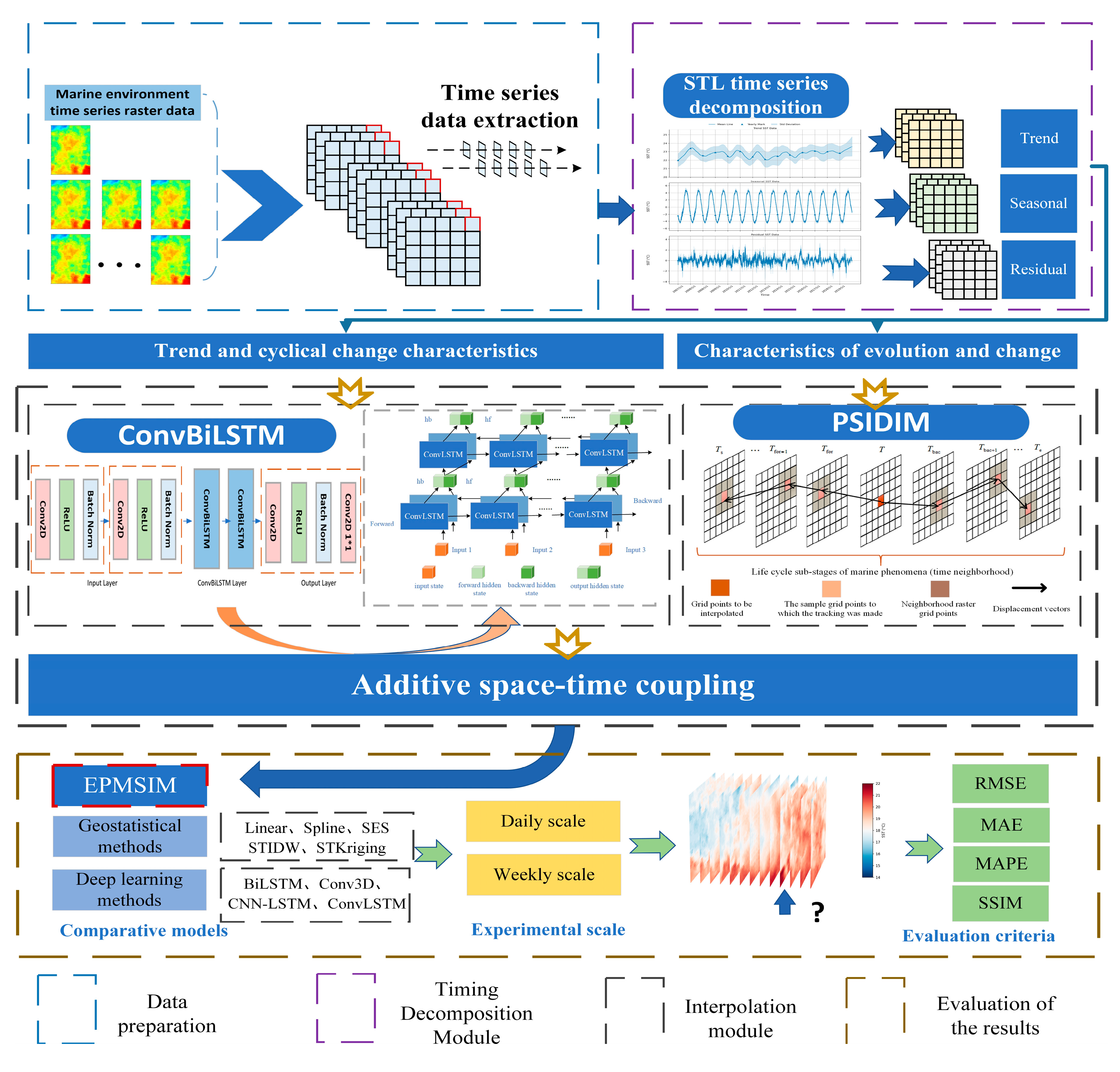
Figure 2.
Schematic diagram of ConvBiLSTM structure.
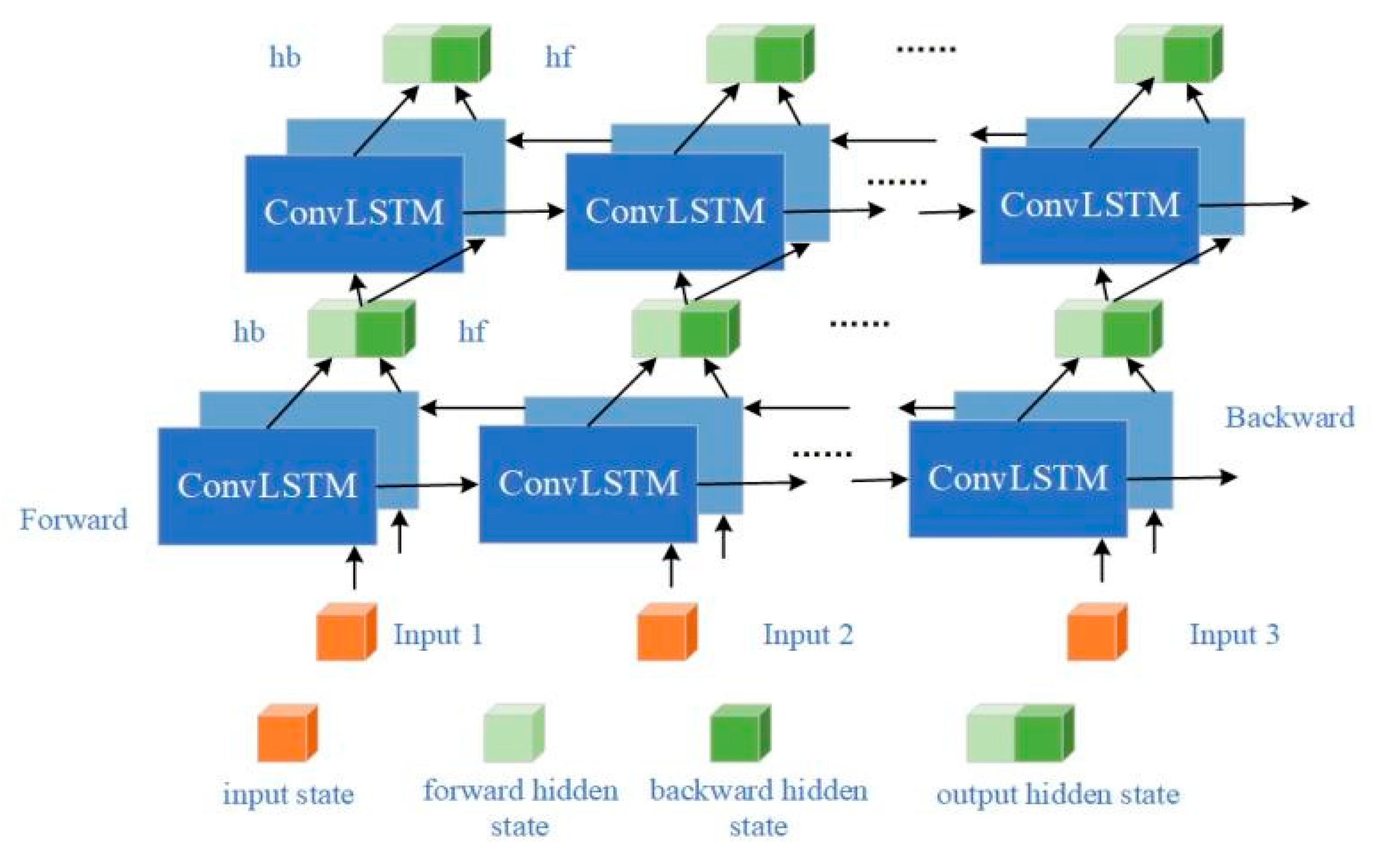
Figure 3.
Schematic diagram of PSDTIM principle.
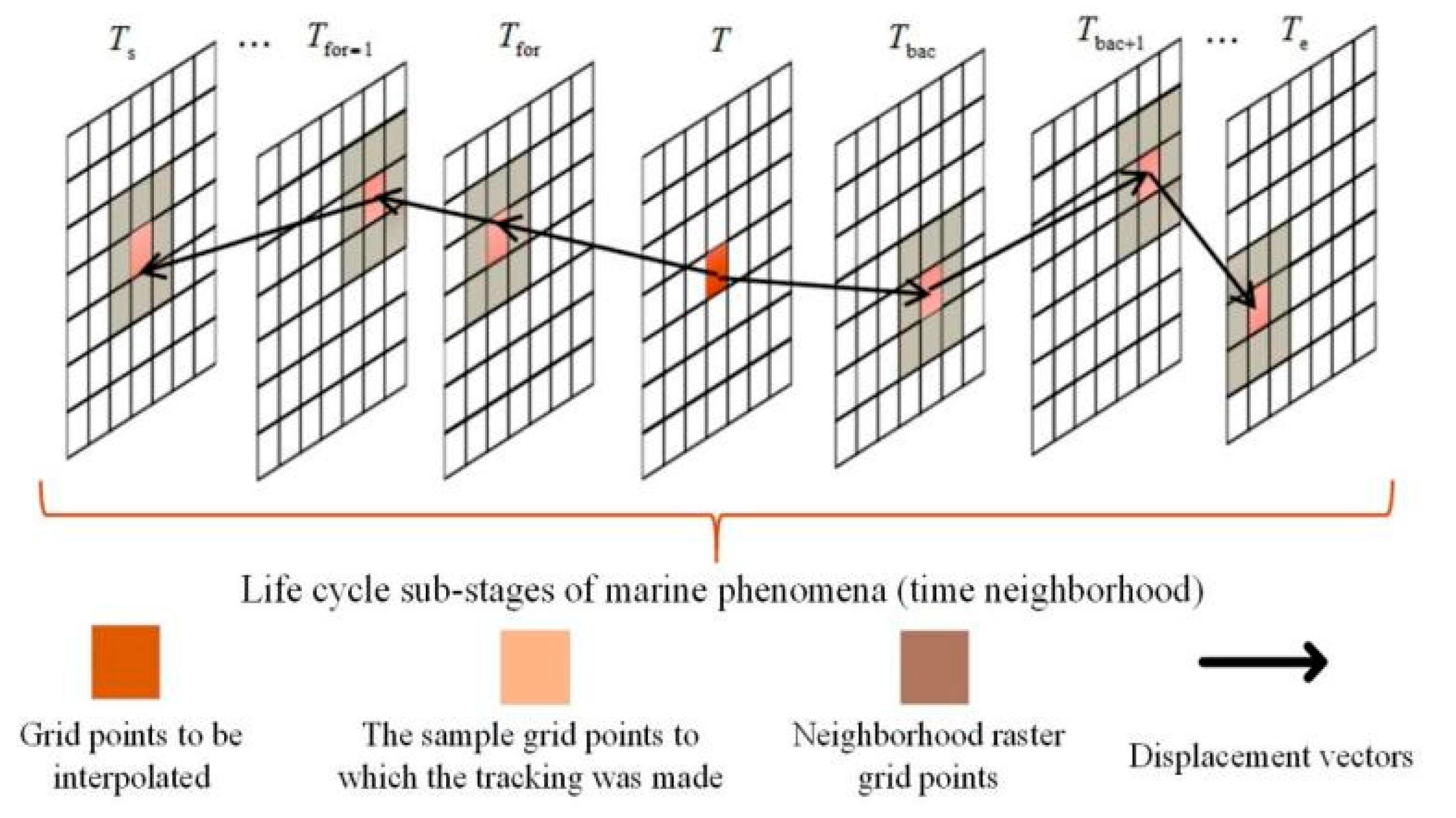
Figure 4.
The blue box indicates the location of the study area. The background shows the annual average sea temperature of 2006. On the right are the selected sequence images of the mesoscale eddy case at 3-day intervals.
Figure 4.
The blue box indicates the location of the study area. The background shows the annual average sea temperature of 2006. On the right are the selected sequence images of the mesoscale eddy case at 3-day intervals.
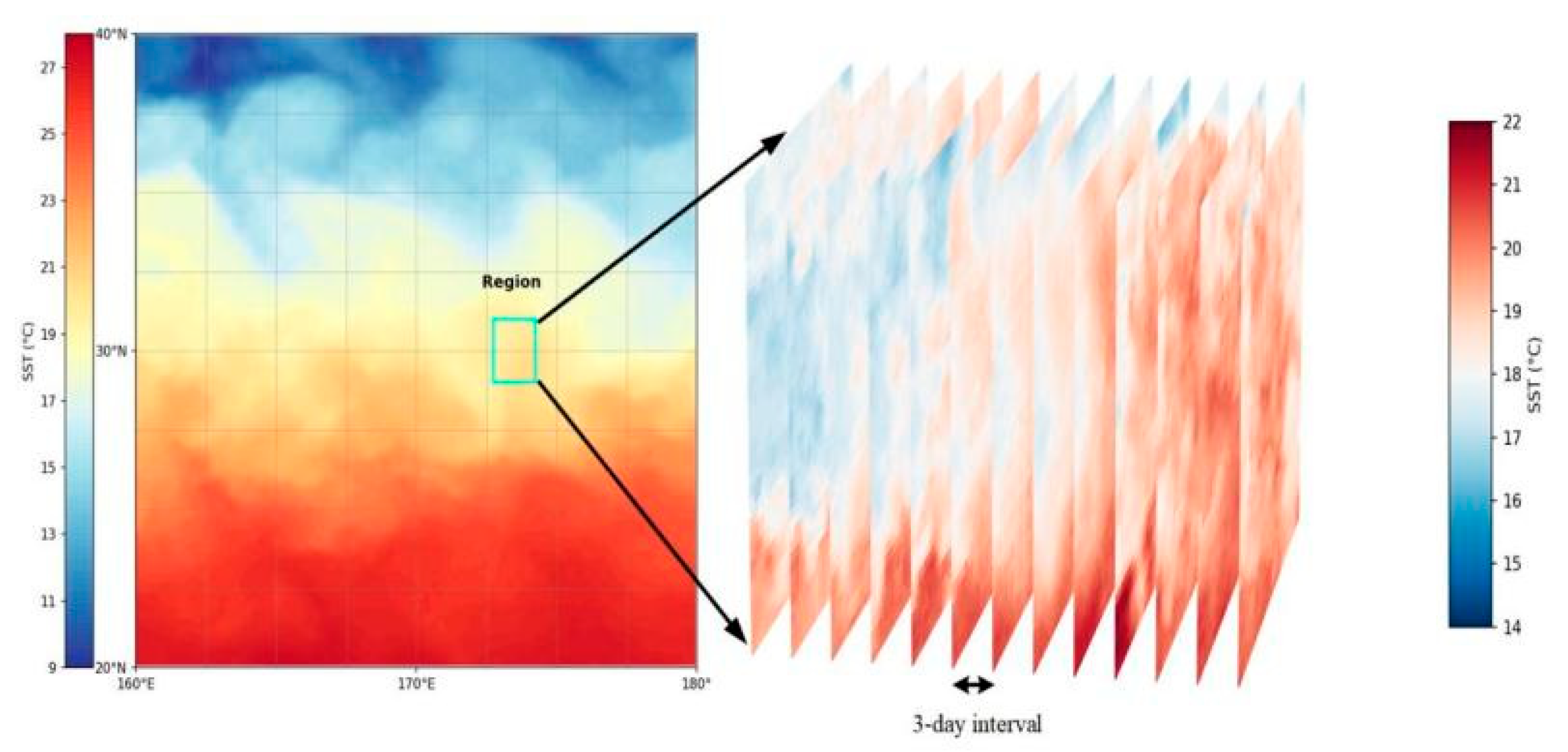
Figure 5.
Average schematic of the STL decomposition at the daily scale for all grid points in the study area using the original data. The solid line represents the average value curve, the shaded area indicates the spatial standard deviation, and the triangle symbols represent the markers at one-year intervals.
Figure 5.
Average schematic of the STL decomposition at the daily scale for all grid points in the study area using the original data. The solid line represents the average value curve, the shaded area indicates the spatial standard deviation, and the triangle symbols represent the markers at one-year intervals.
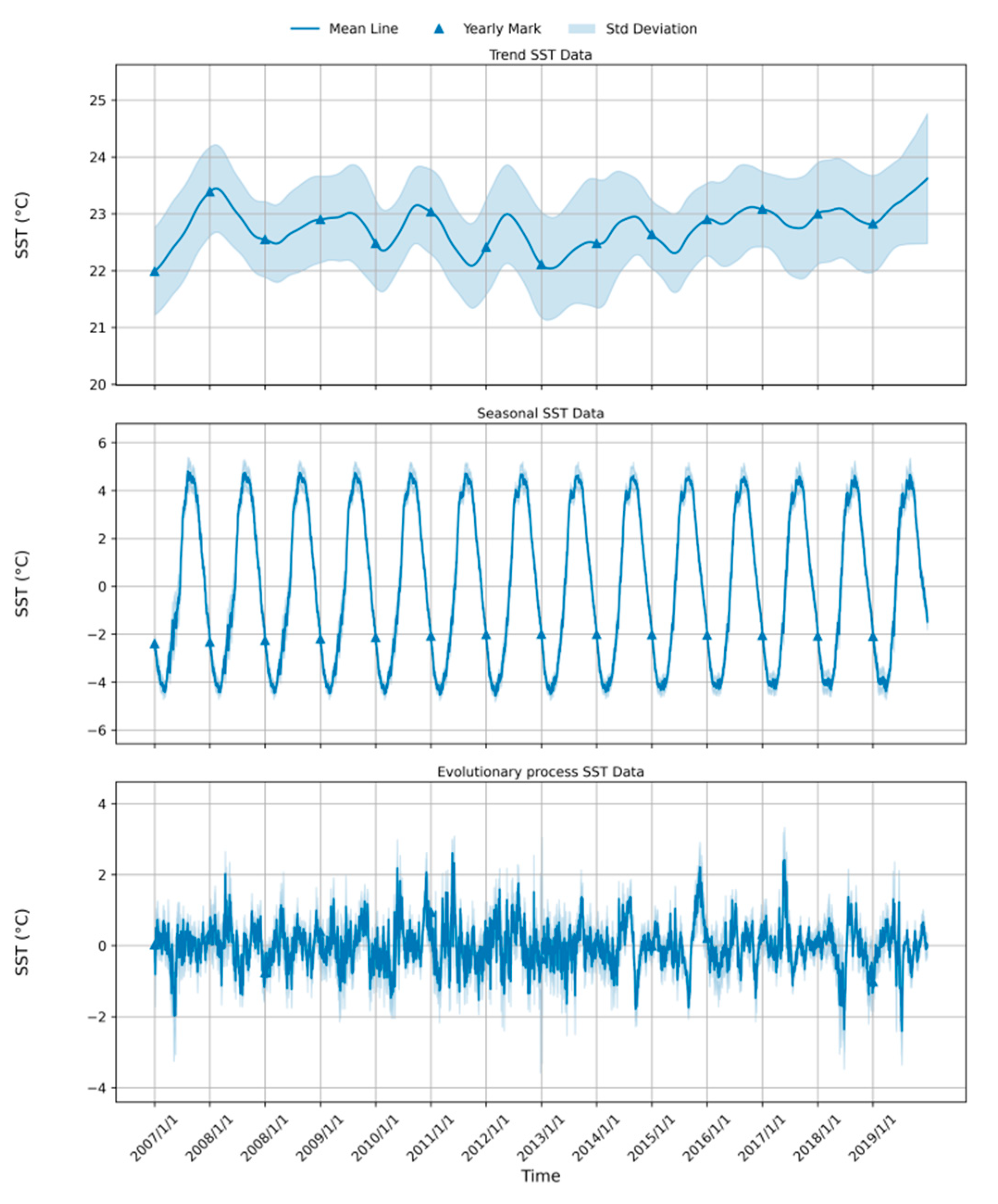
Figure 6.
Visualization of different interpolation results for the eddy case at the daily scale.
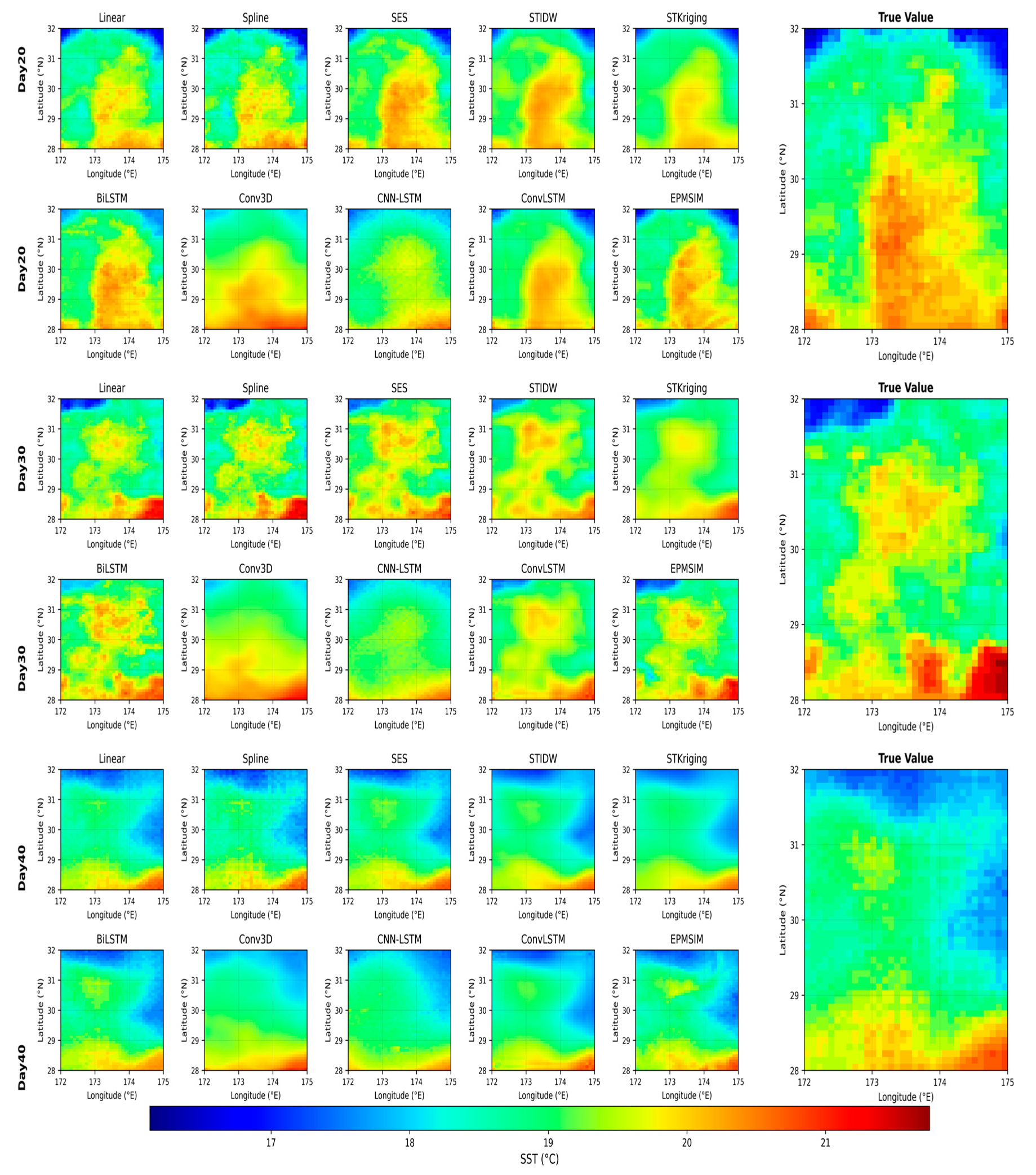
Figure 7.
Scatter plot of different interpolation results for the eddy case at the daily scale.
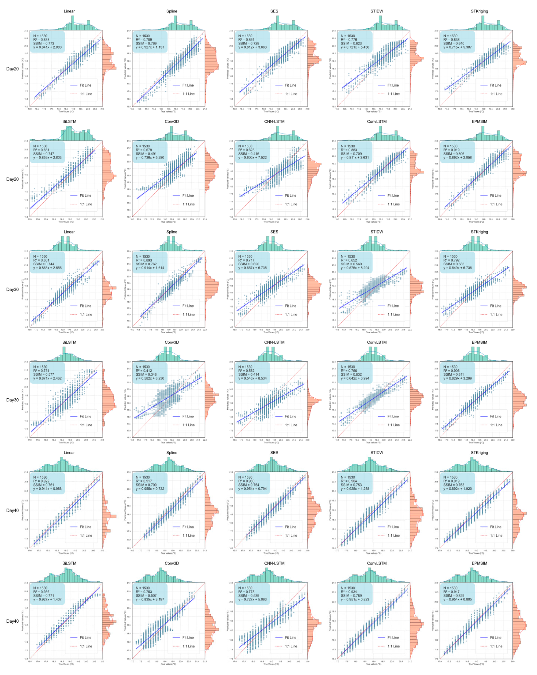
Figure 8.
Visualization of SST interpolation errors for the eddy case at the daily scale. The deeper the color (red or blue) in the figure, the greater the difference between the interpolation results and the ground truth in that area.
Figure 8.
Visualization of SST interpolation errors for the eddy case at the daily scale. The deeper the color (red or blue) in the figure, the greater the difference between the interpolation results and the ground truth in that area.
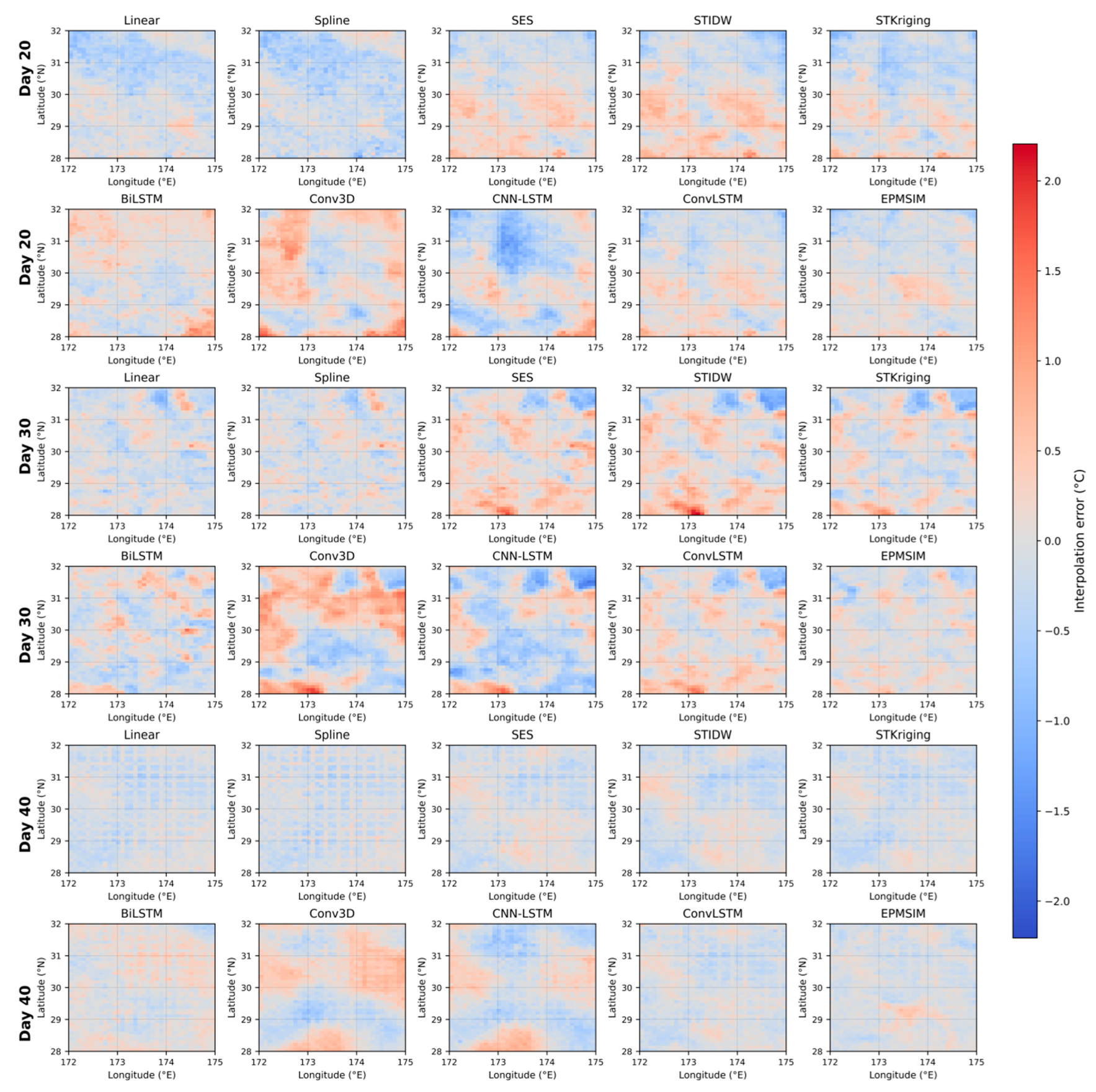
Figure 9.
The four radar charts correspond to the SSIM values at the interpolation time points for four different interpolation experiments: (a) daily-scale eddy case, (b) daily-scale non-eddy case, (c) weekly-scale eddy case, (d) weekly-scale non-eddy case.
Figure 9.
The four radar charts correspond to the SSIM values at the interpolation time points for four different interpolation experiments: (a) daily-scale eddy case, (b) daily-scale non-eddy case, (c) weekly-scale eddy case, (d) weekly-scale non-eddy case.

Figure 10.
Performance of the integrated coupling ablation experiment for the mesoscale eddy case at the daily scale: (a) RMSE; (b) MAE; (c) MAPE.
Figure 10.
Performance of the integrated coupling ablation experiment for the mesoscale eddy case at the daily scale: (a) RMSE; (b) MAE; (c) MAPE.
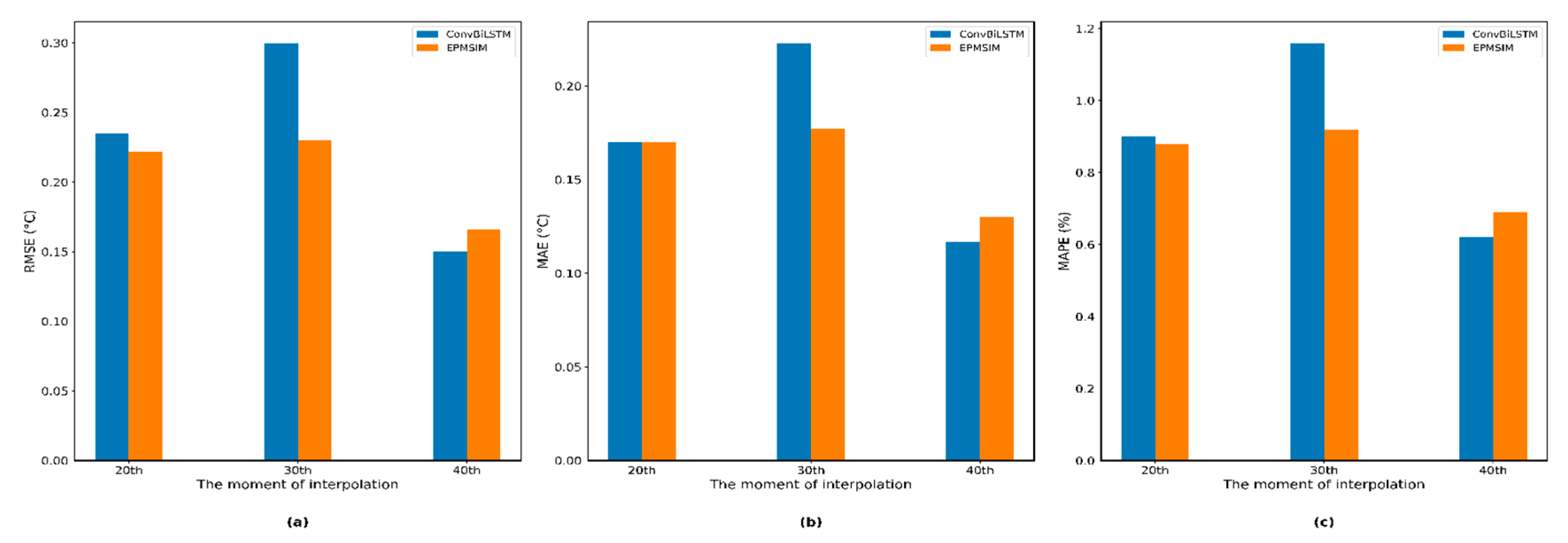
Figure 11.
Performance of the integrated coupling ablation experiment for the non-mesoscale eddy case at the daily scale: (a) RMSE; (b) MAE; (c) MAPE.
Figure 11.
Performance of the integrated coupling ablation experiment for the non-mesoscale eddy case at the daily scale: (a) RMSE; (b) MAE; (c) MAPE.
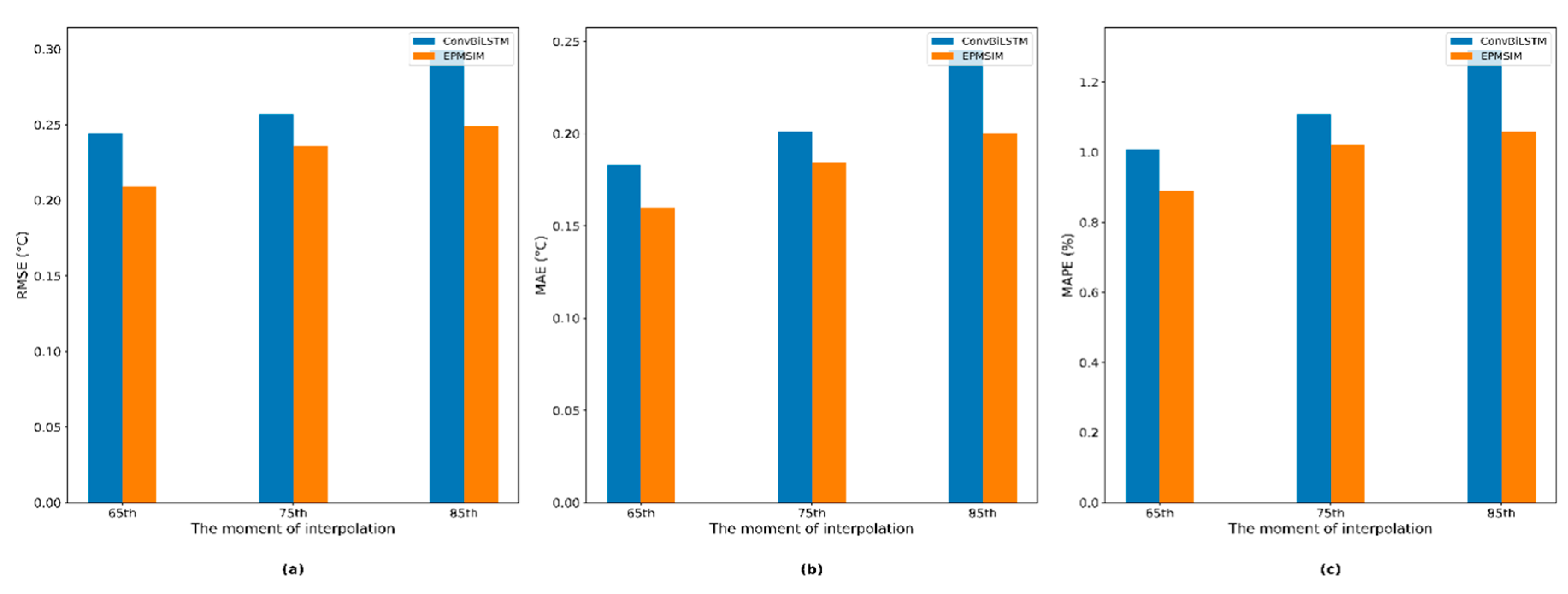
Figure 12.
Ablation experiment performance for the daily-scale mesoscale eddy case: (a) RMSE; (b) MAE; (c) MAPE.
Figure 12.
Ablation experiment performance for the daily-scale mesoscale eddy case: (a) RMSE; (b) MAE; (c) MAPE.
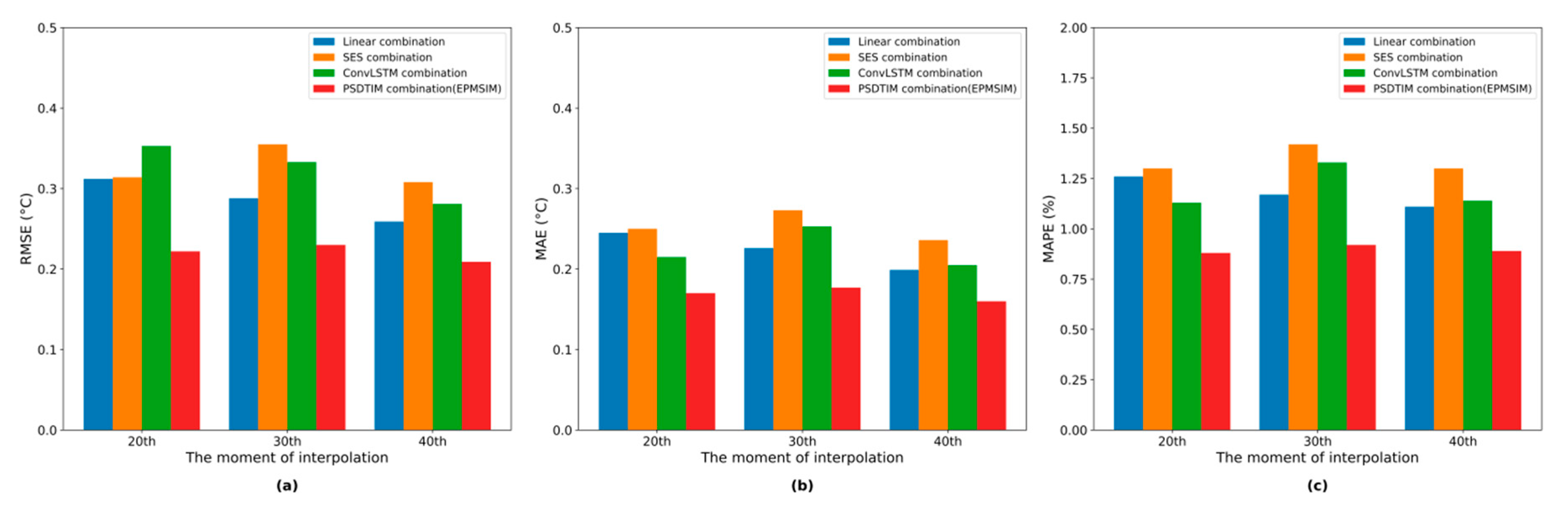
Figure 13.
Ablation experiment performance for the daily-scale non-mesoscale eddy case: (a) RMSE; (b) MAE; (c) MAPE.
Figure 13.
Ablation experiment performance for the daily-scale non-mesoscale eddy case: (a) RMSE; (b) MAE; (c) MAPE.
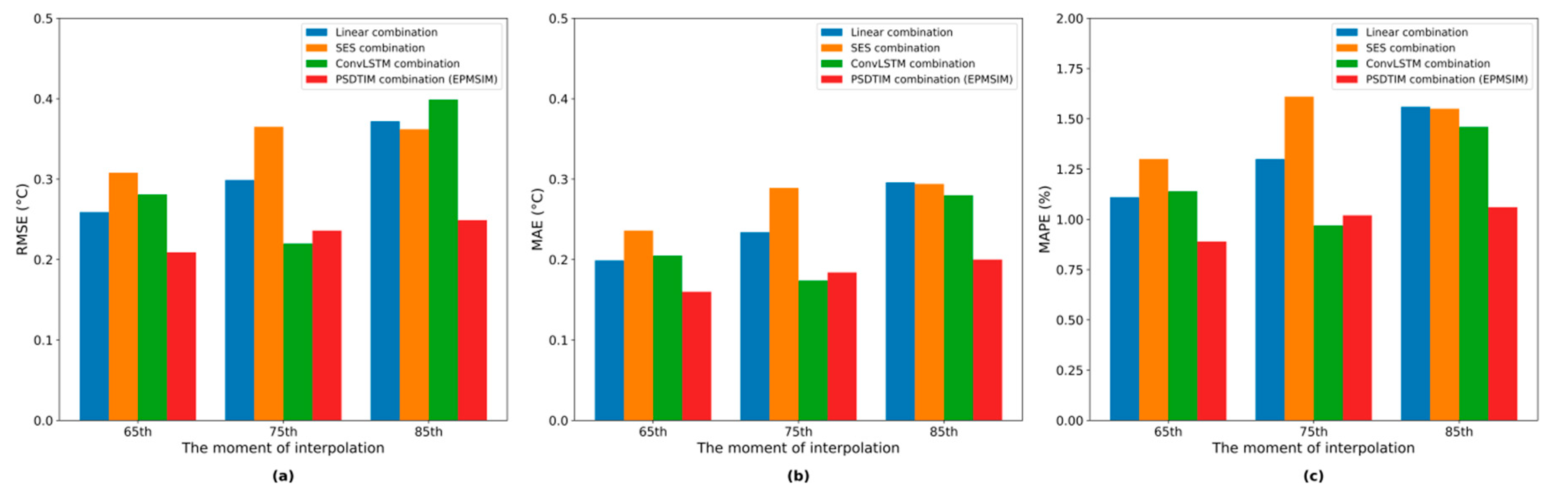

Table 1.
Model composition.
| Function | Pathway | Layer composition |
| Feature extraction Layer | Block 1 | 3×3 Convolution ReLU Batch normalization |
| Block 2 | 3×3 Convolution ReLU Batch normalization |
|
| ConvBiLSTM Layer | Block 3 | ConvBiLSTM Dropout |
| Block 4 | ConvBiLSTM Dropout |
|
| Output Layer | Block 5 | 3×3 Convolution ReLU Batch normalization 1×1 Convolution |
Table 2.
The data statistics for the study area at different scales in 2006.
| Data | Maximum | Minimum | Range | Mean | Standard Deviation |
| Daily- scale | 28.50 | 15.45 | 13.04 | 22.06 | 3.07 |
| Weekly- scale | 28.35 | 15.75 | 12.60 | 22.07 | 3.06 |
Table 3.
Comparisons among different methods for the eddy area at the daily scale .
| Methods | the 20th day | the 30th day | the 40th day | ||||||
| RMSE/ ℃ |
MAE/ ℃ |
MAPE/ % |
RMSE/ ℃ |
MAE/ ℃ |
MAPE/ % |
RMSE/ ℃ |
MAE/ ℃ |
MAPE/ % |
|
| Linear | 0.313 | 0.244 | 1.25 | 0.261 | 0.199 | 1.03 | 0.201 | 0.155 | 0.82 |
| Spline | 0.358 | 0.291 | 1.50 | 0.248 | 0.191 | 1.00 | 0.208 | 0.162 | 0.86 |
| SES | 0.287 | 0.229 | 1.20 | 0.402 | 0.313 | 1.64 | 0.190 | 0.152 | 0.81 |
| STIDW | 0.368 | 0.295 | 1.55 | 0.447 | 0.337 | 1.76 | 0.223 | 0.180 | 0.96 |
| STKriging | 0.312 | 0.250 | 1.30 | 0.345 | 0.264 | 1.37 | 0.205 | 0.166 | 0.88 |
| BiLSTM | 0.286 | 0.213 | 1.13 | 0.324 | 0.250 | 1.33 | 0.182 | 0.142 | 0.76 |
| Conv3D | 0.441 | 0.341 | 1.80 | 0.581 | 0.483 | 2.54 | 0.358 | 0.295 | 1.59 |
| CNN-LSTM | 0.487 | 0.379 | 1.96 | 0.516 | 0.417 | 2.16 | 0.346 | 0.287 | 1.53 |
| ConvLSTM | 0.266 | 0.211 | 1.10 | 0.366 | 0.283 | 1.48 | 0.185 | 0.149 | 0.79 |
| EPMSIM | 0.222 | 0.170 | 0.88 | 0.230 | 0.177 | 0.92 | 0.166 | 0.130 | 0.69 |
Table 4.
Comparisons among different methods for the non-eddy area at the daily scale.
| Methods | the 65th day | the 75th day | the 85th day | ||||||
| RMSE/ ℃ |
MAE/ ℃ |
MAPE/ % |
RMSE/ ℃ |
MAE/ ℃ |
MAPE/ % |
RMSE/ ℃ |
MAE/ ℃ |
MAPE/ % |
|
| Linear | 0.241 | 0.182 | 1.02 | 0.269 | 0.199 | 1.10 | 0.277 | 0.224 | 1.18 |
| Spline | 0.229 | 0.174 | 0.97 | 0.299 | 0.227 | 1.27 | 0.211 | 0.166 | 0.89 |
| SES | 0.318 | 0.237 | 1.31 | 0.365 | 0.292 | 1.64 | 0.462 | 0.390 | 2.07 |
| STIDW | 0.349 | 0.261 | 1.45 | 0.388 | 0.324 | 1.81 | 0.644 | 0.553 | 2.91 |
| STKriging | 0.310 | 0.240 | 1.34 | 0.308 | 0.247 | 1.37 | 0.427 | 0.356 | 1.87 |
| BiLSTM | 0.299 | 0.220 | 1.23 | 0.321 | 0.243 | 1.36 | 0.339 | 0.245 | 1.35 |
| Conv3D | 0.435 | 0.354 | 1.98 | 0.329 | 0.264 | 1.48 | 0.385 | 0.311 | 1.64 |
| CNN-LSTM | 0.418 | 0.332 | 1.85 | 0.348 | 0.278 | 1.54 | 0.328 | 0.269 | 1.44 |
| ConvLSTM | 0.311 | 0.239 | 1.32 | 0.338 | 0.272 | 1.52 | 0.323 | 0.252 | 1.34 |
| EPMSIM | 0.209 | 0.160 | 0.89 | 0.236 | 0.184 | 1.02 | 0.249 | 0.200 | 1.06 |
Table 5.
Comparisons among different methods for the eddy area at the weekly scale.
| Methods | the 6th week | the 7th week | the 8th week | ||||||
| RMSE/ ℃ |
MAE/ ℃ |
MAPE/ % |
RMSE/ ℃ |
MAE/ ℃ |
MAPE/ % |
RMSE/ ℃ |
MAE/ ℃ |
MAPE/ % |
|
| Linear | 0.291 | 0.229 | 1.21 | 0.230 | 0.182 | 0.97 | 0.376 | 0.300 | 1.63 |
| Spline | 0.359 | 0.284 | 1.50 | 0.315 | 0.243 | 1.30 | 0.376 | 0.295 | 1.60 |
| SES | 0.795 | 0.657 | 3.23 | 1.143 | 0.975 | 4.78 | 0.599 | 0.488 | 2.69 |
| STIDW | 0.571 | 0.459 | 2.44 | 0.702 | 0.623 | 3.37 | 0.683 | 0.556 | 3.05 |
| STKriging | 0.359 | 0.279 | 1.49 | 0.341 | 0.280 | 1.52 | 0.440 | 0.343 | 1.88 |
| BiLSTM | 0.499 | 0.428 | 2.20 | 0.438 | 0.360 | 1.88 | 0.371 | 0.297 | 1.60 |
| Conv3D | 0.470 | 0.372 | 1.99 | 0.411 | 0.311 | 1.69 | 0.438 | 0.350 | 1.91 |
| CNN-LSTM | 0.385 | 0.316 | 1.67 | 0.319 | 0.265 | 1.43 | 0.347 | 0.280 | 1.52 |
| ConvLSTM | 0.570 | 0.473 | 2.53 | 0.370 | 0.288 | 1.54 | 0.433 | 0.344 | 1.88 |
| EPMSIM | 0.250 | 0.193 | 1.01 | 0.191 | 0.160 | 0.86 | 0.284 | 0.229 | 1.22 |
Table 6.
Comparisons among different methods for the non-eddy area at the weekly scale . .
| Methods | the 12th week | the 13th week | the 14th week | ||||||
| RMSE/ ℃ |
MAE/ ℃ |
MAPE/ % |
RMSE/ ℃ |
MAE/ ℃ |
MAPE/ % |
RMSE/ ℃ |
MAE/ ℃ |
MAPE/ % |
|
| Linear | 0.561 | 0.494 | 2.82 | 0.366 | 0.313 | 1.70 | 0.356 | 0.270 | 1.46 |
| Spline | 0.632 | 0.556 | 3.17 | 0.611 | 0.547 | 2.98 | 0.624 | 0.546 | 2.97 |
| SES | 0.556 | 0.451 | 2.60 | 0.552 | 0.457 | 2.46 | 0.714 | 0.636 | 3.43 |
| STIDW | 0.554 | 0.450 | 2.59 | 0.600 | 0.509 | 2.74 | 0.417 | 0.345 | 1.86 |
| STKriging | 0.513 | 0.429 | 2.47 | 0.386 | 0.324 | 1.74 | 0.278 | 0.232 | 1.25 |
| BiLSTM | 0.480 | 0.398 | 2.20 | 0.772 | 0.690 | 3.95 | 0.300 | 0.246 | 1.34 |
| Methods | the 12th week | the 13th week | the 14th week | ||||||
| RMSE/ ℃ |
MAE/ ℃ |
MAPE/ % |
RMSE/ ℃ |
MAE/ ℃ |
MAPE/ % |
RMSE/ ℃ |
MAE/ ℃ |
MAPE/ % |
|
| Conv3D | 0.386 | 0.325 | 1.85 | 0.339 | 0.267 | 1.43 | 0.397 | 0.324 | 1.73 |
| CNN-LSTM | 0.295 | 0.241 | 1.34 | 0.344 | 0.282 | 1.53 | 0.258 | 0.212 | 1.14 |
| ConvLSTM | 0.420 | 0.336 | 1.92 | 0.578 | 0.497 | 2.68 | 0.285 | 0.228 | 1.24 |
| EPMSIM | 0.240 | 0.200 | 1.13 | 0.327 | 0.277 | 1.50 | 0.258 | 0.195 | 1.06 |
Disclaimer/Publisher’s Note: The statements, opinions and data contained in all publications are solely those of the individual author(s) and contributor(s) and not of MDPI and/or the editor(s). MDPI and/or the editor(s) disclaim responsibility for any injury to people or property resulting from any ideas, methods, instructions or products referred to in the content. |
© 2026 by the authors. Licensee MDPI, Basel, Switzerland. This article is an open access article distributed under the terms and conditions of the Creative Commons Attribution (CC BY) license (http://creativecommons.org/licenses/by/4.0/).
Copyright: This open access article is published under a Creative Commons CC BY 4.0 license, which permit the free download, distribution, and reuse, provided that the author and preprint are cited in any reuse.


