Bayesian Analysis of Tuberculosis Spread Scenarios in Regions of Russian Federation

1. Mathematical Modeling of the Tuberculosis Spread

Despite some success in the fight against Tuberculosis in the Russian Federation and in the world, the disease remains one of the main challenges to national healthcare systems, being the leading global cause of death from infectious diseases, one of the 10 main causes of death and the predominant cause of death in people infected with HIV. According to WHO, last year 10.6 million people fell ill with Tuberculosis for the first time, 1.3 million people died, the number of MDR cases increased by 3% [1,2]. For successful control over the spread of socially significant and epidemically dangerous infectious diseases such as Tuberculosis, predictive mathematical modeling of the epidemic process is necessary, capable of providing a reliable forecast of the probability of developing an unfavorable and favorable scenario of the epidemic situation in specific territories and early planning/implementation of the necessary interventions [3].

The difficulty of developing a model of slow infections dynamics (HIV/AIDS, Tuberculosis) is to consider the heterogeneity of the population with various climatic, environmental, epidemiological, medical and biological, socio-economic characteristics, including migration, demographic characteristics of regions, availability of medical services, the presence of high-risk groups (HIV-infected people, people with chronic diseases, addiction to psychoactive substances, etc.) and a high proportion of drug-resistant strains.

The models used for the dynamics of infectious diseases in populations have varying degrees of complexity, but three main approaches and their combinations can be distinguished [4]. The first approach is to divide the population into non-overlapping, homogeneously mixed groups with respect to infection and to introduce rules for transition from one group to another. [5]. Typically, models of this type are systems of integral, integro-differential and difference equations (SIR models), interconnected by the mass action law. In the review [5] examples of SIR models and their features in describing the dynamics of Tuberculosis in a population are given. Such models are characterized by their parameters (coefficients and initial conditions), and describe an outbreak of an infectious disease if coefficients are constant. Accounting for medical and socio-economic interventions is possible in a generalized manner, while detailing the features of related processes is difficult.

In work [6] It is shown that the parameter of Tuberculosis infectiousness is sensitive to morbidity, therefore demographic and socio-economic indicators were introduced as a step function into the change of infectiousness parameter. This approach is demonstrated in predicting morbidity in the regions of the Russian Federation and confirms that the change of socio-economic conditions in the regions is one of the reasons for the decrease of Tuberculosis spread. Furthermore this effect is combined with the results of the work of the anti-Tuberculosis services. In work [7] for the model of Tuberculosis and HIV co-infection, fundamental scenarios of the disease spread were constructed with regulating the parameter of the effectiveness of treatment in the regions of the Russian Federation. However, including socio-economic processes in an explicit form requires modification of the model (introduction of additional equations) and data. The second approach is agent based modeling (e.g. [8]). Within this framework, each individual of the population is described by a set of parameters (age, immune status, time elapsed since infection, etc.), the rules of interaction of individuals and the influence of the environment. This approach allows us to obtain a more detailed picture of the epidemic process: age stratification of morbidity, the influence of social status and the environment on the incidence and prevalence of infection, changes in immunity as a result of the spread of infection, etc. To specify models of this type, both differential equations and algorithmic descriptions are used. Such models are computationally expensive and require a detailed description specific to the region under consideration, however, the results of modeling and forecasting are not only advisory, but also practical for medical organizations (e.g. [9]).

The third approach to describing and forecasting of infectious diseases spread relies on statistical data and deep learning models. However, their implementation requires complete data of the process under study, which is difficult to obtain for slowly progressing infections (for example, when modeling and forecasting COVID-19, the effectiveness of such models is studied in the works [10,11]).

To build scenarios for the spread of Tuberculosis in the regions of the Russian Federation, it is necessary to take into account the heterogeneity of its distribution [12], as well as the large percentage of multidrug-resistant forms of Tuberculosis (MDR-TB) in the Siberian regions of the Russian Federation among newly diagnosed patients (see Figure 1). For example, more than 40% of newly diagnosed patients were MDR-TB infected in the Novosibirsk region in 2024. While the average figure for the Siberian Federal District fluctuates around 30%.

The inclusion of the incipient and subclinical TB (ISbTB) compartment is crucial for modeling TB elimination, as it represents a major obstacle to ending TB alongside latent TB [13]. This form is characterized by a low, oscillating bacterial load, qualifying as paucibacillary disease [14], yet remains sufficient for transmission, especially in prolonged close contact [15]. Such individuals are significant concealed community sources of infection [16], eluding diagnosis due to low bacterial burdens that cause false-negative results [17] and present a ”hard to determine” category [18].

ISbTB escalates the total epidemic contagiousness; its basic reproduction number, even if low, contributes to the continuity of the overall TB epidemic process. Furthermore, these forms can harbor drug resistance [19] and lead to relapse post-treatment [20]. Despite its proven epidemiological significance, many models omit this parameter. Our model aims to address this gap.

In the recent years the modeling of the epidemics is also developed with stochastic approach, also with stochastic control strategies [21,22].

The interest in mathematical modeling of TB was strongly elevated after the issue of WHO concept of ending TB by 2030 [23]. WHO tuberculosis researchers published a mathematical model to predict TB incidence decline with fulfillment of the Sustainable Development Goal (SDG) subtargets [24]. In the study [25] the susceptible-exposed-infectious-recovered (SEIR) model with different age groups was developed and the feature of heterogeneity considered in the model allowed to assess the effect of age as a factor on TB transmission and more accurately determine parameters for ending TB. Separate studies have considered the effects of drug-resistant cases [26], time lag [27] and age structure.

Questions of the hidden reservoirs of the TB infection and the burden of overall drug resistance inside them were not significantly involved in mathematical modeling of the TB infection in current literature.

It has recently become clear that traditional notions of dichotomizing tuberculosis infection into latent and active tuberculosis are a simplification that fails to reflect the biological process of transition from infection to disease. To more realistically characterize this process, the concept of two main intermediate groups of patients, existing between infection and active TB, has been introduced: incipient and subclinical TB disease. Therefore, it is now believed that the immediate precursors of the development of active TB are not so much the infection state itself (latent TB, LTBI), but rather those stages of infection progression that directly precede active TB, i.e., incipient and subclinical TB [28,29,30,31]. Recently, the first evidence has emerged of the important role of incipient and subclinical TB in the spread of infection [31,32], however, the actual contribution of these conditions to the TB epidemic remains unclear, as diagnosing them in patients is difficult. Molecular biological methods currently being developed for detecting incipient and subclinical TB will soon be introduced into healthcare practice. These methods will enable a more accurate understanding of the true contribution to the spread of TB and the prognosis of the epidemic. [33,34,35,36,37,38]. Since this contribution depends on numerous dynamic variables influencing the spread of the epidemic (human population characteristics, drug resistance of circulating strains, access to medical care, etc.), it is appropriate to describe scenarios for the impact of incipient and subclinical TB on the epidemic process using mathematical modeling. In our paper we construct the model, for the first time, examines not LTBI, but rather impact of incipient and subclinical TB in TB epidemiology.

This mathematical model based on the comprehensive SEIS-type compartmental model for TB dynamics in the Russian Federation, incorporating multi-drug resistant (MDR) forms, detection processes, and treatment pathways. In the methods we combine differential equation modeling based on M.I. Perelman and G.I. Marchuk ideas [39] as well as Y. Yi et al. model [40], Sobol sensitivity analysis, Bayesian optimization, and MCMC based forecasting, applying the framework to several high burden regions, that are of epidemiological interest in the Russian Federation as the obstacle of ending TB in Russia. The key points of the current publication, that allow to achieve additional results, as comparing with the other authors:

• Parameter identification and optimization with the use of the concept and paradigm of inverse and ill-posed problems allowed us to evaluate the intensity of epidemic process in the risk regions of Russia, that we need to identify with the aim to combat TB as the regional and national high stream.
• Sensitivity-based identifiability analysis allows us to find correlated TB parameters that implicate on the accuracy of parameter identifiability and forecast uncertainty.
• We construct the posterior distribution of sensitive epidemiological parameters of the TB compartmental mathematical model (such as contagiousness of TB contact with bacterioexcretion, the rate of TB activation, the rate of undetected TB contact with bacterioexcretion per year) that allows us to evaluate the expected TB infected people in Russian Federation regions for three years ahead.

If we get robust estimations of epidemic force parameters, we have enough scientific potential to plan counterforce actions including efficient treatment of drug resistance and drug sensitive forms of TB in the amounts enough to concur transmission. The results of the expected heterogeneity of regions and the assessment of key epidemiological parameters are consistent with the results of the works of A.A. Romanyukha [9] and O.A. Melnichenko [6], and also expand and clarify the uncertainty due to the inclusion of incipient and subclinical TB forms, i.e. the key ideas of this paper are

• Inclusion of detection stages based on papers [6,9] and add new compartments of MDR-TB based on [40];
• Inclusion of incipient/subclinical TB as a compartment based on [41];
• Usage of Sobol sensitivity analysis and Bayesian MCMC for uncertainty quantification;
• Region-specific posterior parameter estimation.

The paper is organized as follows: in the Section 2 we formulate the differential SIR-type model, give analysis of stability of stationary points of the model, formulate the problem of parameters identification and provide sensitivity analysis. In the Section 3 the statistical data used on Tuberculosis incidence, socio-economic characteristics of the regions of the Russian Federation and their processing for use in modeling are presented. In the Section 4 numerical estimates of the probability distribution of epidemiological parameters based on statistical data and SIR model data, as well as scenarios for the spread of Tuberculosis in the regions of the Russian Federation are presented.

2. SEIS Model of Tuberculosis Dynamics with Multiple Drug-Resistant Forms

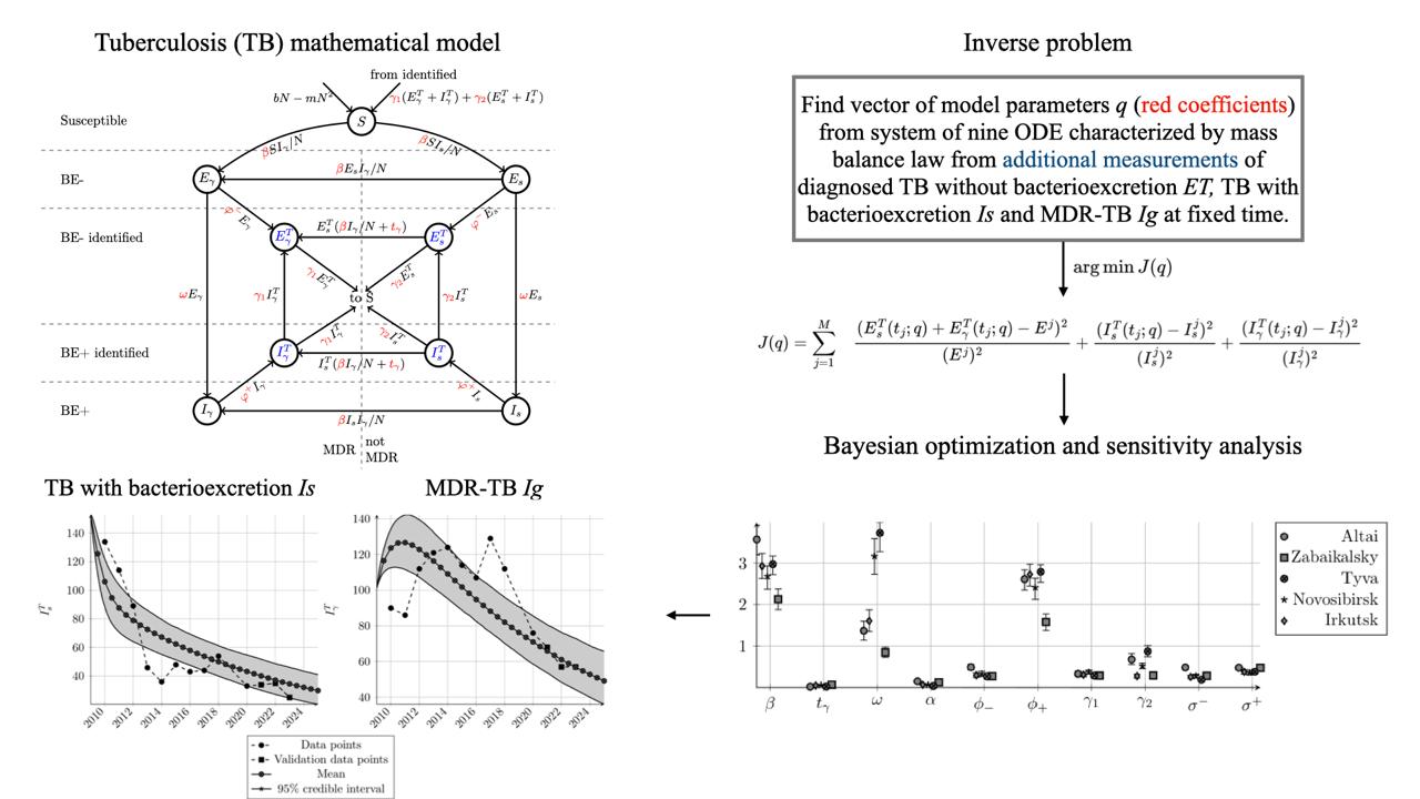
The mathematical model of Tuberculosis (TB) spread and control used in this paper is based on the approach proposed by G.I. Marchuk and A.A. Romanyukha in 2004 [39] and paper by A.A. Romanyukha [41] concerning the TB detection. Using the law of mass action, we formulate the SEIS model [40], characterized by a system of 9 ordinary differential equations (the model diagram is shown in Figure 2):

$$\left\{\begin{array}{cc}\hfill {\displaystyle \frac{dS}{dt}}& =-\beta S(I_s+I_{\gamma })/N+{\gamma }_1(E_{\gamma }^T+I_{\gamma }^T)+{\gamma }_2(E_s^T+I_s^T)+bN-m{N}^2-\mu S;\hfill \\ \hfill {\displaystyle \frac{d{E}_s}{dt}}& =\beta S{I}_s/N-\omega E_s-{\phi }^{-}{E}_s-\beta E_s{I}_{\gamma }/N-\mu E_s;\hfill \\ \hfill {\displaystyle \frac{d{E}_s^T}{dt}}& =-{\gamma }_2{E}_s^T+{\gamma }_2{I}_s^T+{\phi }^{-}{E}_s-E_s^T(\beta I_{\gamma }/N+t_{\gamma })-\mu E_s^T;\hfill \\ \hfill {\displaystyle \frac{d{E}_{\gamma }}{dt}}& =\beta S{I}_{\gamma }/N-\omega E_{\gamma }-{\phi }^{-}{E}_{\gamma }+\beta E_s{I}_{\gamma }/N-\mu E_{\gamma };\hfill \\ \hfill {\displaystyle \frac{d{E}_{\gamma }^T}{dt}}& ={\gamma }_1{I}_{\gamma }^T-{\gamma }_1{E}_{\gamma }^T+{\phi }^{-}{E}_{\gamma }+E_s^T(\beta I_{\gamma }/N+t_{\gamma })-\mu E_{\gamma }^T;\hfill \\ \hfill {\displaystyle \frac{d{I}_s}{dt}}& =\omega E_s-{\phi }^{+}{I}_s-\beta I_s{I}_{\gamma }/N-(\alpha +\mu )I_s;\hfill \\ \hfill {\displaystyle \frac{d{I}_s^T}{dt}}& =-2{\gamma }_2{I}_s^T+{\phi }^{+}{I}_s-I_s^T(\beta I_{\gamma }/N+t_{\gamma })-(\alpha +\mu )I_s^T;\hfill \\ \hfill {\displaystyle \frac{d{I}_{\gamma }}{dt}}& =\omega E_{\gamma }-{\phi }^{+}{I}_{\gamma }+\beta I_s{I}_{\gamma }/N-(\alpha +\mu )I_{\gamma };\hfill \\ \hfill {\displaystyle \frac{d{I}_{\gamma }^T}{dt}}& =-2{\gamma }_1{I}_{\gamma }^T+{\phi }^{+}{I}_{\gamma }+I_s^T(\beta I_{\gamma }/N+t_{\gamma })-(\alpha +\mu )I_{\gamma }^T\hfill \end{array}\right.$$

(1)

with initial conditions

$$\begin{array}{c}\hfill \begin{array}{c}S\left(0\right)=S_0,E_s\left(0\right)=E_0^s,E_s^T\left(0\right)=E_{0T}^s,\hfill \\ E_{\gamma }\left(0\right)=E_0^{\gamma },E_{\gamma }^T\left(0\right)=E_{0T}^{\gamma },I_s\left(0\right)=I_0^s,\hfill \\ I_s^T\left(0\right)=I_{0T}^s,I_{\gamma }\left(0\right)=I_0^{\gamma },I_{\gamma }^T\left(0\right)=I_{0T}^{\gamma }.\hfill \end{array}\end{array}$$

(2)

Here $N=S\left(t\right)+E_s\left(t\right)+E_s^T\left(t\right)+E_{\gamma }\left(t\right)+E_{\gamma }^T\left(t\right)+I_s\left(t\right)+I_s^T\left(t\right)+I_{\gamma }\left(t\right)+I_{\gamma }^T\left(t\right)$ is a volume of the studied population that satisfies the logistic equation:

$${\displaystyle \frac{dN}{dt}}=(b-\mu )\left(1-{\displaystyle \frac{N}{k}}\right)N-\alpha (I_s+I_{\gamma }+I_s^T+I_{\gamma }^T).$$

Here $b-\mu >0$, $bN-m{N}^2$ refers to the influx of susceptible individuals into the population due to the birth rate or immigration, $m=(b-\mu )/k$, k is a population potential.

The population is divided into nine non-overlapping groups according to Figure 2 (the subscript ^T denotes the group of detected infected individuals). The description of the variables and parameters of the model is given in Table 1.

This model is based on the following principles for Russian Federation:

• TB BE- and TB BE+ forms are distinguished, and TB BE- is considered an early stage of the disease preceding the development of severe TB BE+ stages;
• We assume treated individuals return to full susceptibility S, consistent with evidence of high reinfection rates in high-incidence settings [43,44];
• patients are divided into detected and undetected;
• the proportion of those cured from TB with bacterial excretion can transit to a form without bacterial excretion;
• the probability of transition from forms without MDR to TB-MDR is nonlinear;
• during treatment of TB BE+ infected people can transit to both latent forms S and TB BE- with equal probability.

A part of TB patients who successfully complete treatment, when the symptoms have disappeared and bacterial excretion has stably stopped, undergo recurrence. In the Siberian Federal District in 2024 the recurrence rate among those cured averages 33% (in different regions – from 20 to 43% [45]). This means that cured patients remain susceptible to developing TB infection. TB recurrence results from immunological deficiency (dependent on risk factors such as unfavorable social, medical and stress factors, etc.) and is caused by either relapse of an original infection or exogenous reinfection with a new or the same strain of M. tuberculosis. The source of relapse is bacteria that remain in a persistent, viable state in cured (BE-) persons for many months and years within post-TB residual lung foci, lymph nodes, or even within hematopoietic or mesenchymal stem cells [46,47,48,49]. The source of reinfection is bacteria acquired through continued contacts of cured patients with people with subclinical or active TB [32,44]. In addition, indirect evidence that cured patients remain in a TB-sensitive risk group is that IGRA tests after cure remain positive in the absolute majority of cases for decades and even until the end of life [50].

Within the framework of the model, all populations, regardless of status, are subject to average mortality rate with the parameter $\mu$. A susceptible or latent infected individual from group S moves to the infected non-bacterial stage $E_s$ (or closed form of TB) after contact with an TB infected without MDR $I_s$ governing the contagiousness parameter $\beta$ or to the TB infected non-bacterial stage with MDR $E_{\gamma }$. Infected closed-form TB $E_s$, $E_{\gamma }$ migrate to the bacterial form with $\omega$ probability. Infected patients without MDR can migrate to infected MDR-TB with $t_{\gamma }$ probability, and also with rate $\beta$ when in contact with infected TB without bacterioexcretion. In the model, each group of TB infected people is divided into detected (with index T) and undetected with expression coefficients ${\phi }^{-}$ for TB BE-, MDR-TB BE- and ${\phi }^{+}$ for TB BE+, MDR-TB BE+, respectively. In the model, additional mortality of infected people with bacterioexcretion $\alpha$ is observed and they move to the state S with probabilities ${\gamma }_1$ (for form with MDR) and ${\gamma }_2$.

The model principle construction was based on real infection reserwars. This is TB with bacterioexcretion and TB without bacterioexcretion - the incipient and subclinical TB, the latter always bearing a real hazard of converting to bacterioexcretion clinical form. That does not mean, that we exclude significance of latent TB, especially in HIV-infected individuals, but consider this of lower value and as perspective of further studies with the focci of the ending TB.

The limits of the change in the parameters of the models, that are used in linear parts of equations, were determined from statistics (TB-infected registration form No. 33). For example, the proportion of identified non-MDR TB cured in 1 year, ${\gamma }_2$ in a linear approximation is inversely proportional to the time spent in therapy. That is, the limits ${\gamma }_2\in [0.3,2]$ correspond to $[0.5,3.33]$ years undergoing therapy for TB+ non-MDR patients.

Restrictions on initial conditions in the regions of the Russian Federation are also assumed, namely the percentage of undetected infected people is less than 50% due to the absence of a sharp outbreak of TB:

$$\begin{array}{c}\hfill E_0^s={\sigma }^{-}{E}_{0T}^s,E_0^{\gamma }={\sigma }^{-}{E}_{0T}^{\gamma },\\ \hfill I_0^s={\sigma }^{+}{I}_{0T}^s,I_0^{\gamma }={\sigma }^{+}{I}_{0T}^{\gamma }.\end{array}$$

2.1. ODE System Analysis

The behavior of the ODE systems is broadly studied from the perspective of asymptotic properties, and this paper is also the case. We note that for such systems it is often possible to find analytical solution using Lie algebra [51], however it is effectively applicable only for smaller systems, or systems with symmetries. Thus, the model considered is too complicated for this approach, so we present only the results of stationary points stability.

For the derivation of stationary points of the system (1), only in this section we assume that ${\gamma }_1={\gamma }_2=\gamma$. Let us consider the system obtained from the system (1) by adding the equations and replacing:

$$\begin{array}{c}\hfill I=I_s+I_{\gamma },I^T=I_s^T+I_{\gamma }^T,\\ \hfill E=E_s+E_{\gamma },E^T=E_s^T+E_{\gamma }^T.\end{array}$$

Then we obtain the following system:

$$\begin{array}{c}\hfill \left\{\begin{array}{cc}{\displaystyle \frac{dS}{dt}}\hfill & =bN-m{N}^2-\beta SI/N+\gamma I^T-\mu S;\hfill \\ {\displaystyle \frac{dE}{dt}}\hfill & =\beta SI/N-(\mu +\omega +{\phi }^{-})E;\hfill \\ {\displaystyle \frac{d{E}^T}{dt}}\hfill & ={\phi }^{-}E+\gamma I^T-\mu E^T;\hfill \\ {\displaystyle \frac{dI}{dt}}\hfill & =\omega E-(\alpha +\mu +{\phi }^{+})I;\hfill \\ {\displaystyle \frac{d{I}^T}{dt}}\hfill & ={\phi }^{+}I-(2\gamma +\alpha +\mu )I^T.\hfill \end{array}\right.\end{array}$$

(3)

Lemma 1. 

The system (3) has the only stationary state that is trivial.

Proof. 

By equating the right-hand sides to 0, we obtain a system for finding stationary solutions:

$$\begin{array}{c}\hfill \left\{\begin{array}{cc}\beta SI/N+\mu S\hfill & =bN-m{N}^2+\gamma I^T;\hfill \\ (\mu +\omega +{\phi }^{-})E\hfill & =\beta SI/N;\hfill \\ \mu E^T+\gamma I^T\hfill & ={\phi }^{-}E;\hfill \\ (\alpha +\mu +{\phi }^{+})I\hfill & =\omega E;\hfill \\ (2\gamma +\alpha +\mu )I^T\hfill & ={\phi }^{+}I.\hfill \end{array}\right.\end{array}$$

(4)

From 2 and 4 equations of system 4, we obtain:

$$S={\displaystyle \frac{(\mu +\omega +{\phi }^{-})(\alpha +\mu +{\phi }^{+})}{\beta \omega }}N.$$

Therefore, we are left with equations 1, 3 and 5 of system (4) with a single nonlinear term $N^2$.

Note that $N\left(0\right)<k$, then $\forall t:N\left(t\right)<k$.

In the edge cases, when $N\ll k$ or $N\approx k$ we obtain linear system for stationary point, thus, it is unique (except for the trivial point). As soon as the solution is confined, it may tend towards one of these solutions.

We rewrite the system (4) the following way:

$$\begin{array}{c}\hfill \left\{\begin{array}{cc}(\mu +\omega +{\phi }^{-})E+\mu S=bN-m{N}^2\hfill & +\gamma I^T;\hfill \\ E^T=I({\phi }^{-}(\alpha +\mu +{\phi }^{+})/\omega \hfill \\ -\gamma {\phi }^{+}/(2\gamma +\alpha +\mu ))/\mu \hfill & =I{c}_{Et};\hfill \\ E=I(\alpha +\mu +{\phi }^{+})/\omega \hfill & =I{c}_E;\hfill \\ I^T=I{\phi }^{+}/(2\gamma +\alpha +\mu )\hfill & =I{c}_{It}.\hfill \end{array}\right.\end{array}$$

As soon as $dN/dt$: $bN-m{N}^2=\alpha (I+I^T)$, and for the first equation, we get:

$$\begin{array}{cc}\hfill (\mu +\omega +{\phi }^{-})I{c}_E+\mu S& =\alpha I(1+c_{It})+\gamma I{c}_{It}.\end{array}$$

Thus,

$$\begin{array}{cc}\hfill I& =-{\displaystyle \frac{\mu S}{(\mu +\omega +{\phi }^{-})c_E-\alpha (1+c_{It})-\gamma c_{It}}}=c_{I}S.\end{array}$$

Then, as soon as $dN/dt=0$, we get:

$$\begin{array}{c}\hfill (b-\mu )\left(1-{\displaystyle \frac{N}{k}}\right)N-\alpha (I+I^T)=0\end{array}$$

Thus,

$$\begin{array}{c}\hfill N=k\left(1-{\displaystyle \frac{\alpha c_S{c}_I(1+c_{It})}{b-\mu }}\right).\end{array}$$

(5)

That means that there is unique stationary point, except for the trivial and disease-free. However, by substitution of coefficients $c_S,c_I,c_E,c_{It}$ into (5), we obtain $N=0$ and this point coincides with the trivial point (checked with Wolfram Mathematica, the code is available in GiHub repository). □

Our model operates in absolutes and reflects the logistic curve of the population growth. Most human populations in the regions of the Russian Federation show slow population dynamics and in these dynamics the nontrivial stationary state of TB prevalence can exist. However, we can apply the model to the risk groups where fast growth and diminution can occur.

2.1.1. Stationary Points Stability

The matrix of linearized system (4):

$$\left(\begin{array}{ccccc}b-2mN-{\displaystyle \frac{\beta I(N-S)}{N^2}}-\mu & b-2mN& b-2mN& b-2mN-{\displaystyle \frac{\beta S(N-I)}{N^2}}& b-2mN+\gamma \\ {\displaystyle \frac{\beta I(N-S)}{N^2}}& -\mu -\omega -{\phi }^{-}& 0& {\displaystyle \frac{\beta S(N-I)}{N^2}}& 0\\ 0& {\phi }^{-}& -\mu & 0& \gamma \\ 0& \omega & 0& -\alpha -\mu -{\phi }^{+}& 0\\ 0& 0& 0& {\phi }^{+}& -2\gamma -\alpha -\mu \end{array}\right)$$

(6)

There are two stationary points $N=0$ and $S=N=k$.

Then from the form of (6) with $I=0$, point $S=N=k$ is stable, when

$$\mu <band(\mu +\omega +{\phi }^{-})(\alpha +\mu +{\phi }^{+})<\beta \omega$$

(7)

and point $N=0$ is stable when $b-\mu <0$, or $\mu >b$.

In our examples we will consider cases $b<\mu$ and $b\approx \mu$, what depicts the situation in Russian Federation [52]. That means that the point $N=0$ is globally stable and the stability analysis of stationary points is not informative, since the difference $\mu -b$ is quite small and thus the convergence to the point $N=0$ is slow, so we are interested in short-term dynamics (compared to the convergence to stationary point).

The 10-year window may seem too large for short-term forecasting; however, that is not the case for Tuberculosis and the current difference between birth and mortality rates. The Tuberculosis has the infectivity rate around 2-4 and recovery rate around 0.1 (for annual time scale). It indicates that the Tuberculosis infection characteristic duration time is around 10 years. The difference between birth and mortality rate is too small (0.003), that implies that the solution will reach the point with $N=0$ in more than 4000 years if the rates stay constant.

2.1.2. Basic Reproduction Number ${\mathcal{R}}_0$

To derive the basic reproduction number ${\mathcal{R}}_0$, we consider two states of people in the system (1): infected without MDR $x_1={(E_s,E_s^T,I_s,I_s^T)}^{\mathrm{T}}$ and with MDR-TB $x_2={(E_{\gamma },E_{\gamma }^T,I_{\gamma },I_{\gamma }^T)}^{\mathrm{T}}$ at the disease free equilibrium (DFE) point ${\mathcal{E}}_0=(k,0,0,0,0,0,0,0,0)$, i.e. $S_0=N=k$. Following the approach from the article [53], we derive the basic reproduction number for non-MDR TB ${\mathcal{R}}_1$ and MDR-TB ${\mathcal{R}}_2$.

We rewrite the system (1) as follows:

$$\dot{x_i}=(f_i-v_i)x_i,i=1,2,$$

where $f_i$ characterize infection in the group due to external flows, $v_i$ – recovery, mortality in the group. Then we have:

$$\begin{array}{cc}\hfill f_1& =\left(\begin{array}{c}\beta S{I}_s/N\\ 0\\ 0\\ 0\end{array}\right),v_1=\left(\begin{array}{c}{\displaystyle \frac{\beta E_s{I}_{\gamma }}{N}}+\omega E_s+{\phi }^{-}{E}_s+\mu E_s\\ {\displaystyle \frac{\beta E_s^T{I}_{\gamma }}{N}}+{\gamma }_2{E}_s^T-{\gamma }_2{I}_s^T-{\phi }^{-}{E}_s+t_{\gamma }{E}_s^T+\mu E_s^T\\ {\displaystyle \frac{\beta I_s{I}_{\gamma }}{N}}-\omega E_s+{\phi }^{+}{I}_s+(\alpha +\mu )I_s\\ {\displaystyle \frac{\beta I_s^T{I}_{\gamma }}{N}}+2{\gamma }_2{I}_s^T-{\phi }^{+}{I}_s+t_{\gamma }{I}_s^T+(\alpha +\mu )I_s^T\end{array}\right).\hfill \\ \hfill f_2& =\left(\begin{array}{c}{\displaystyle \frac{\beta S{I}_{\gamma }}{N}}+{\displaystyle \frac{\beta E_s{I}_{\gamma }}{N}}\\ {\displaystyle \frac{\beta E_s^T{I}_{\gamma }}{N}}\\ {\displaystyle \frac{\beta I_s{I}_{\gamma }}{N}}\\ {\displaystyle \frac{\beta I_s^T{I}_{\gamma }}{N}}\end{array}\right),v_2=\left(\begin{array}{c}\omega E_{\gamma }+{\phi }^{-}{E}_{\gamma }+\mu E_{\gamma }\\ {\gamma }_1{E}_{\gamma }^T-{\gamma }_1{I}_{\gamma }^T-{\phi }^{-}{E}_{\gamma }-t_{\gamma }{E}_s^T+\mu E_{\gamma }^T\\ -\omega E_{\gamma }+{\phi }^{+}{I}_{\gamma }+(\alpha +\mu )I_{\gamma }\\ 2{\gamma }_1{I}_{\gamma }^T-{\phi }^{+}{I}_{\gamma }-t_{\gamma }{I}_s^T+(\alpha +\mu )I_{\gamma }^T\end{array}\right).\hfill \end{array}$$

For the linearized system $\dot{x_i}=(F_i-V_i)x_i$, $i=1,2$, we calculate the Jacobian matrices

$$F_i={\displaystyle \frac{\partial f_k}{\partial x_i^j}}\left({\mathcal{E}}_0\right),V_i={\displaystyle \frac{\partial v_k}{\partial x_i^j}}\left({\mathcal{E}}_0\right),j,k=1,\dots ,4,$$

after which we find the eigenvalues of the matrices product: $\lambda \left(F_i{V}_i^{-1}\right)$, $i=1,2$. The matrices $F_i$ and $V_i$ are presented in Appendix A.1.

Thus, we get

$${\mathcal{R}}_1={\mathcal{R}}_2={\displaystyle \frac{\beta \omega }{(\omega +{\phi }^{-}+\mu )({\phi }^{+}+\alpha +\mu )}}.$$

As soon as ${\mathcal{R}}_0=max\{{\mathcal{R}}_1,{\mathcal{R}}_2\}$, the basic reproduction number in the model (1) has the form

$$\begin{array}{c}\hfill {\mathcal{R}}_0={\displaystyle \frac{\beta \omega }{(\omega +{\phi }^{-}+\mu )({\phi }^{+}+\alpha +\mu )}}.\end{array}$$

(8)

The basic reproduction number ${\mathcal{R}}_0$ is based on infectious rates (contagiousness of TB, rate of undetected TB, rate of TB BE- turning into BE+). The difference between the MDR and non-MDR strains in the model (1) is the rate of treatment, which is not reflected in the basic reproduction number (since it describes the rate of infection in a non-immune population). The identical ${\mathcal{R}}_0$ suggests that, in the absence of treatment, MDR and non-MDR spread similarly. This highlights the role of treatment in controlling MDR.

Lemma.The stationary point without infection ${\mathcal{E}}_0$ is stable when basic reproduction number (8) ${\mathcal{R}}_0<1$.

The ${\mathcal{R}}_0<1$ in Lemma means, that $\beta \omega <(\omega +{\phi }^{-}+\mu )({\phi }^{+}+\alpha +\mu )$. It coincides with part of (7), that represents stability with respect to infection outbreak.

The exclusion of latent forms of TB increases the basic reproduction number ${\mathcal{R}}_0$, namely, due to undetected infectiousness and the transition to an active form (it is possible that such a transition may not occur during the simulation), the ${\mathcal{R}}_0$ will decrease (see details in Appendix A.1).

2.2. Inverse Problem

We assume that additional information about solution in fixed points in time is given:

$$\begin{array}{c}\hfill \begin{array}{c}{E}_s^T\left(t_j\right)+E_{\gamma }^T\left(t_j\right)+{\epsilon }_j=E^j,\hfill \\ I_s^T\left(t_j\right)+{\epsilon }_j=I_s^j,I_{\gamma }^T\left(t_j\right)+{\epsilon }_j=I_{\gamma }^j,\hfill \\ j=1,\dots ,M.\hfill \end{array}\end{array}$$

(9)

Then the inverse problem (1), (2), (9) is to identify the parameters of the SEIS model $q=(\beta ,{\gamma }_1,{\gamma }_2,\omega ,t_{\gamma },\alpha ,{\phi }^{-},{\phi }^{+},{\sigma }^{-},{\sigma }^{+})\in {\mathbb{R}}_{+}^{10}$ with the help of additional information (9).

We assume that observations $y_t=(E_s^T+E_{\gamma }^T,I_s^T,I_{\gamma }^T)$ are subject to independent additive Gaussian errors:

$$y_t=f_t\left(q\right)+{\epsilon }_t,{\epsilon }_t\sim \mathcal{N}(0,\Sigma ).$$

Here $f_t\left(q\right)=(E_s^T(t;q)+E_{\gamma }^T(t;q),I_s^T(t;q),I_{\gamma }^T(t;q))$, $\Sigma =\mathrm{diag}({\sigma }_1^2,{\sigma }_2^2,{\sigma }_3^2)$ and ${\sigma }_i$ are estimated jointly with q.

The model (1) is theoretically identifiable based on algebra analysis [54].

Due to the instability and non-uniqueness of the solution to the inverse problem, the following section presents a sensitivity analysis of the model, which will allow us to estimate the degree of sensitivity of the parameters q to the measured states of the system (9) [55].

2.3. Sensitivity-Based Identifiability Analysis for SEIS Model

The sensitivity analysis of the model (1) was carried out using the Sobol method [56], with a uniform distribution of parameters, the variation limits of which are given in Table 1. This method quantifies how the variance in model outputs (predictions of TB diagnoses) can be apportioned to individual parameters and their interactions across the entire apriori feasible parameter space. The initial conditions (2) approximate the epidemiological situation of the Novosibirsk region in 2009:

$$\begin{array}{cc}& N=2263383,E_s=300,E_{\gamma }=500,\\ & E_s^T=1100,E_{\gamma }^T=1549,\\ & I_s=100,I_{\gamma }=400,I_s^T=438,I_{\gamma }^T=1330.\end{array}$$

Thus, $S=N-E_s-E_{\gamma }-E_s^T-E_{\gamma }^T-I_s-I_{\gamma }-I_s^T-I_{\gamma }^T=2257666$ people. The modeling time is 10 years.

For a model outputs as we consider in inverse problems $y_1=E_s^T(t;q)+E_{\gamma }^T(t;q)$, $y_2=I_s^T(t;q)$, $y_3=I_{\gamma }^T(t;q)$ (see measurement 9) the Sobol decomposition expresses the total variance $V\left(y_n\right)$, $n=1,2,3$:

$$\begin{array}{c}\hfill V^{\left(n\right)}=V\left(y_n\right)=\sum _i{V}_i^{\left(n\right)}+\sum _{i<j}{V}_{ij}^{\left(n\right)}+\dots +V_{1\dots m}^{\left(n\right)},n=1,2,3.\end{array}$$

Here $V_i^{\left(n\right)}=V\left[\mathrm{E}\left(y_n\right|q_i)\right]$, $i=1,\dots ,10$, is the first-order (main) effect variance, measuring the contribution of parameter $q_i$ alone, $V_{ij}^{\left(n\right)}$ is the second-order interaction variance between $q_i$ and $q_j$, and so on for higher-order interactions.

We compute the total-order Sobol index

$$S_{T_i}^{\left(n\right)}={\displaystyle \frac{V^{\left(n\right)}-V\left[\mathrm{E}\left(y_n\right|{\mathbf{q}}_{\sim i})\right]}{V^{\left(n\right)}}},n=1,2,3,$$

and the first-order and second order Sobol indexes

$$S_{1_i}^{\left(n\right)}={\displaystyle \frac{V_i^{\left(n\right)}}{V^{\left(n\right)}}},S_{ij}^{\left(n\right)}={\displaystyle \frac{V_{ij}^{\left(n\right)}}{V^{\left(n\right)}}},n=1,2,3,$$

where ${\mathbf{q}}_{\sim i}$ denotes all parameters except $q_i$, $1=1,\dots ,10$. $S_{T_i}^{\left(n\right)}$ measures the total contribution of $q_i$, including all its interactions with other parameters. A parameter with very low total-order indices $S_{T_i}^{\left(n\right)}$ (e.g., $<0.01$) has a negligible influence on the measurements $y_n$, $n=1,2,3$. Its value cannot be inferred from the data. If $S_{T_i}^{\left(n\right)}>0.5$ for some $q_i$ to data $y_n$ than total contribution of $q_i$, including all its interactions with other parameters is significant. However, if $S_{T_i}^{\left(n\right)}>0.5$ and $S_{1_i}^{\left(n\right)}<0.5$ than parameter $q_i$ may still be identifiable, but its estimate will be strongly correlated with others.

We use Sensitivity Analysis Library in Python (SALib package) and set $N=1024·(2·8+2)=18432$ Sobol samples. In Figure 3 (right) the total-order Sobol coefficients are given for the model coefficients $\tilde{q}=(\beta ,{\gamma }_1,{\gamma }_2,\omega ,t_{\gamma },\alpha ,{\phi }^{-},{\phi }^{+})\in {\mathbb{R}}_{+}^8$ (without initial conditions), including the first indices, the second (correlation), etc. with 95% confidence intervals. The most sensitive to measurements of detected infected is the TB contagiousness parameter $\beta$. The TB detection parameter BE+ ${\phi }^{+}$ is sensitive to infected TB BE+ without MDR $I_s^T\left(t_j\right)$. The proportion of infected TB converting to the BE+ form $\omega$ is sensitive to infected TB-MDR BE+ with and without MDR. The additional mortality rate $\alpha$ due to TB is sensitive to MDR-TB BE+ measurements.

Note, that the first Sobol index for $\beta$ coefficient $S_1^{\left(1\right)}$ for TB BE- measurement is more than 0.5 (this parameter is sensitive to the $y_1$), other ones are less than 0.5 that means the parameter’s influence is primarily through interactions (see Figure 3 left). Its may still be identifiable, but its estimate will be strongly correlated with others. The second Sobol indexes $S_{\beta \omega }^{\left(2\right)}$, $S_{\beta \omega }^{\left(3\right)}$, $S_{\beta {\phi }^{+}}^{\left(2\right)}$ more than 0.2 and $S_{\beta j}^{\left(2\right)}$ close to 0.1-0.2 for all parameters j (see correlation matrices in the Appendix A.2).

As we note that Sobol indices show strong parameter correlations, the formal practical identifiability analysis is performed, i.e. we construct the correlation matrix (see Table 2 for Novosibirsk region) based on the Fisher information matrix

$${\rho }_{ij}={\displaystyle \frac{FI{M}_{ij}^{-1}}{\sqrt{FI{M}_{ii}^{-1}FI{M}_{jj}^{-1}}}},$$

where

$$FIM={\left({\displaystyle \frac{\partial f_t}{\partial q}}\right)}^T{\Sigma }^{-1}{\displaystyle \frac{\partial f_t}{\partial q}}$$

and ${\displaystyle \frac{\partial f_t}{\partial q}}$ is a sensitivity matrix.

Table 2 shows that the parameters with $|{\rho }_{ij}|>0.95$ are difficult to distinguish. For example, ${\rho }_{\beta {\phi }^{+}}>0.98$ indicates that the data cannot independently inform the parameters $\beta$ and ${\phi }^{+}$, only their product is well-identified. That are shown during the sensitivity Sobol analysis as well.

3. Data Analysis

The birth b and mortality $\mu$ rates are presented in Table 3 and Table 4 for five regions of Russian Federation.

To restore parameters of the model for regions of Russian Federation, we used the following data:

• Let $p_{\gamma }=I_{\gamma }^T/(I_{\gamma }^T+I_s^T)$ then from [43], we have data of fraction and absolute number of patients with MDR among the patients with bacillary forms of TB, that represent $p_{\gamma }$ and $I_{\gamma }^T$ respectively.
• From data of form 33 (Information about patients with Tuberculosis from the Order of Rosstat dated 31.12.2010 №483), we have cohorts that represent $I_s^T+I_{\gamma }^T+E_s^T+E_{\gamma }^T=C_{EI}$. Then we may obtain the following:
  • $I_{\gamma }^T$ is given in data;
  • $I_s^T=I_{\gamma }^T(1/p_{\gamma }-1)$;
  • $E_{\gamma }^T+E_s^T=C_{ET}-I_{\gamma }^T-I_s^T$.

For demonstration of the numerical results we choose two regions of Russian Federation with an unfavorable situation in terms of the prevalence of TB: Novosibirsk region and Tyva Republic.

4. Model Scenarios of Tuberculosis Spread

As a result of solving the inverse problem (1), (2), (9), the vector of SEIS model parameters q was determined for each region, the substitution of which into the model (1)-(2) leads to a comparison of the model and real data on identified infected people (Figure 5).

4.1. Bayesian Approach

To obtain the distribution of the model parameters and to construct a forecast considering the uncertainty, we use the Bayesian MCMC (Markov Chain Monte Carlo) approach, in which the posterior distribution for the parameters $q\in {\mathbb{R}}_{+}^{10}$ has the form:

$$p(q\mid y)\propto p(y\mid q)·\prod _{i=1}^{10}p\left(q_i\right).$$

Here $p\left(q_i\right)$ is the prior distributions of the SEIS model parameters, $p(y\mid q)$ is the likelihood of the data.

The likelihood functional is defined by the logarithmic density function of the normal distribution with the mean being the difference of the real data and solution of the direct problem for the given current parameters. The variance of likelihood functional is determined during the MCMC algorithm (see Appendix A.3).

$\beta$$t_{\gamma }$$\omega$$\alpha$${\phi }^{-}$${\phi }^{+}$${\gamma }_1$${\gamma }_2$${\phi }^{-}$${\phi }^{+}$

The results of the inverse problem solution are in Table 5. Parameters with total Sobol index less than 0.01 for all outputs were considered practically non-identifiable and assigned informative Normal priors centered at Optuna values with width 10% of the prior range (see results for mean values in Appendix A.4). The prior distribution $p\left(q_i\right)$ for sensitive parameters $\beta ,{\phi }^{+},\omega$ is proposed as uniform (see Table 1).

We apply the Bayesian approach to find the posteriority distribution of the parameters q with 20000 draws of 4 Markov chains (i.e. 80000 samples for each parameter), mean (column ”Mean”) and 95% credible interval (CI). Differences in the parameters of pathogen contagiousness $\beta$, the proportion of infected TB converting to the BE+ form $\omega$ and the rate of detection ${\phi }^{+}$ of TB infected individuals with bacterial excretion indicate heterogeneity in the prevalence of TB in the Russian Federation regions.

The Pareto front (see Figure A3, Appendix A.5) for three measured statistics (9) shows the uniqueness of the given solution of the inverse problem (TB parameter identification), then the CIs values depend on numerical accuracy the of the correlated parameters.

Figure 4 demonstrates the mean and CI of model parameters as noted in Table 5. Note, that all parameters $\beta ,\omega$ and ${\phi }^{+}$ with wide CI are sensitive to the measurement with its interaction to each other (see Section 2.3), i.e. the total-order Sobol indexes are greater than 0.5, but the first-order indexes are sufficiently small. Scenarios of number of TB BE+ infectious may be unreliable because of $I_s^T$ and $I_{\gamma }^T$ depend on the combination of all these parameters. Small errors in identifying any one of them lead to unrealistic forecasts. Therefore, when analyzing forecast scenarios for TB BE+ groups, it is appropriate to use interval estimates rather than point estimates, as was done in this study. While the model is structurally identifiable, strong parameter correlations (seen in Sobol indices) affect practical identifiability.

In Figure 5, Figure 6 and Figure 7 the probability distribution of TB infected based on Bayesian approach is demonstrated for Novosibirsk region and Tyva Republic of Russian Federation (Figure 5), Altai and Irkutsk regions (Figure 6) as well as Zabaikalskiy region (Figure 7). The approximation for Novosibirsk region is more accurate because of small 95% credible intervals that contain the real data (dashed dot line). The average for all five regions Mean Absolute Percentage Error (MAPE) and Root Mean Square Error (RMSE) are in Table 6. For example, for data $I_s^T$ RMSE=$5·{10}^{-5}$ means that the error is 5 per 100000 people. The single situation when mean prediction is worse is the modeling results for $I_s^T$, what is compensated with adjustments in other groups. The $I_s^T$ forecasts are less accurate only for the Zabaikalsky region, and the data is poorly fit for the Tyva Republic. The Zabaikalsky region data has two ”falls” in data, that cannot be described with the chosen model, as it is able to describe only one peak of infection with descent without additional ”fall”. The Tyva region data has unusual feature of $I_s^T$ being significantly lower than $I_{\gamma }^T$. This may be due to a simplification of the model by ignoring latent tuberculosis infections, which may actually account for some of the detected cases. The basic reproduction number ${\mathcal{R}}_0$, calculated using the formula (8), for all considered regions are close to the 0.9.

We also point out that the data points of 2019 year are not used in inverse problem, because of change in rules of statistical records of TB in Russia [57], which made figures of 2019 year unrepresentative. However, that does not affect the epidemiological process, thus the following years are not affected significantly (see Appendix A.6).

In 2018-early 2019, a surge in TB detection have occurred in the Russian Federation due to the emergence of regulatory official orders that significantly expand the coverage of prophylactic medical examination/observation service and the introduction of modern diagnostic and preventive treatment methods [58,59,60]. We suggest that from 2020 onwards, the impact of these official acts was significantly reduced due to the emergence of the COVID-19 pandemic and, as a result, a decrease in TB detection [61].

A short-term forecast for 3 years ahead was constructed for TB infected with bacterioexcretion BE+. The credible interval and forecast accuracy are higher for TB BE+ without MDR. To improve the accuracy of the MDR-TB BE+ forecast, it is necessary to use a priori information on treatment, immunology, etc. The model cannot capture sudden spikes; forecasts assume stable epidemiological conditions.

5. Discussion

The literature on mathematical modeling of the early stages of untreated pulmonary tuberculosis—its incipient and subclinical forms—is extremely scarce. We found modeling of the early stages of TB in the works of Avilov et al. [41,62], where two models were used, one of which assumes the infectiousness of the initial stages of the disease, and the second considers all cases to be initially non-infectious, but some of them subsequently become infectious. The authors do not give preference to either model, although they consider the first model more plausible. Our model is based on the latest ideas about the very high contagiousness of the early stages of the TB process [32,63], and combines both models, assuming the infectiousness of tuberculosis cases in the early stages and the possible gradual development of some cases to an infectious state. At the same time, like Avilov et al. [5] we defined the development of infectiousness as the transition of patients from the BE- to the BE+ state, which allows us to predict the hidden incidence and prevalence of TB within the framework of the model and to better understand the real epidemic situation in different regions.

Coming through recent ideas in TB forecasting based on statistical methods and statistically based machine learning [3], in our work we also relied on long-term statistical data of departmental reporting for the territories of the Siberian and Far Eastern Federal Districts, being the most unfavorable districts in the Russian Federation. However we used the SEIS type generalized compartment model with the law of mass action and machine learning was added not only to the statistical analysis but precisely to the mathematical model.

We consider the closest work to our research is the study [64]. This prototype model comprises 5 differential equations, as our model has 9 differential equations. The authors used common methodology to derive the formula of $R_0$ and calculate the sensitivity of $R_0$. However, the methodology of comparing the real and the model data is completely different in our works.

The very recent interesting work is presented in [65]. The sensitivity analysis has shown that major positive influence on $R_0$ has the per-capita TB transmission rate, rate of bacteria spread to environment by infectious individuals and the droplet-human propagation coefficient. The negative influence on $R_0$ has the mycobacterium environmental death rate and the transition rate from the low-risk latent TB to high-risk latent TB. Thou in terms of clinical epidemiology the terminology and methodology in our works are quite different, globally we achieved very similar results.

An analysis of the model sensitivity in our model it was shown that the TB contagiousness parameter $\beta$ , the proportion of infected TB converting to the BE+ form $\omega$ and the TB detection parameter BE+ ${\phi }^{+}$ are global sensitive to measurements of the TB BE+ $I_s^T$ , and the first two parameters $\beta$ and $\omega$ are sensitive to the MDR-TB BE+ and TB BE-. The sensitivity is also based on correlations.

Here we fully correspond to the work [66], were the simulation results proved that the key to better prevent and control the spread and develop of TB is to improve the detection rate, and the conversion rate from TB to MDR-TB.

On the Bayesian approach we calculated the credible intervals (CIs) of the posterior distribution of 10 model parameters based for additional information on the number of identified patients with TB BE-, TB BE+ without MDR and MDR-TB BE+ from 2009 to 2021. The less sensitive parameters give small CIs for five considered regions that described the TB propagation and detection in RF regions in common. More sensitive and correlated parameters have huge CIs that proved the heterogeneity of TB propagation in RF regions as well as opens ways for its control. The Pareto front (see Figure A3) for three measured statistics shows the uniqueness of the given solution of the inverse problem (TB parameter identification), then the CIs values depend on numerical accuracy the of the correlated parameters.

Based on identified parameters and its CIs we construct the forecasting scenarios of detected patients with TB BE-, TB BE+ without MDR and MDR-TB BE+ from 2022 to 2026 years for five regions of the Russian Federation, the approach being close to the results [67,68].

6. Conclusion

The aim of our study was to learn the new patterns and laws of TB spreading worldwide on the example of the Russian Federation and to evaluate the combat strategies. In compartment model with revealed and unrevealed cases, incipient and subclinical TB (BE-) and clinical TB (BE+), drug sensitive and drug resistant TB we obtained the formula for the basic reproduction number ${\mathcal{R}}_0$. The formula comprises TB contagiousness parameter $\beta$, rate of TB BE- converting into BE+ $\omega$ and the rate of undetected TB BE+ ${\phi }^{+}$. Using the sensitivity analysis we discovered the leading pattern, determining prevalence of TB clinical forms with bacterial excretion, which are most dangerous for humans in the aspect of lethality and disease transmission. The pattern is based on the same parameters as ${\mathcal{R}}_0$ determinacy, that are TB contagiousness parameter $\beta$, rate of TB BE- converting into BE+ $\omega$ and the rate of undetected TB BE+ clinical forms ${\phi }^{+}$. By solving the inverse problem we proved the variability of these crucial parameters in high incidence regions of the Russian Federation. This heterogeneity is due to differences of medical and social systems. The TB contagiousness parameter $\beta$ depends on intensity of contact tracing. The rate of TB BE- converting into BE+ $\omega$ is influenced by the healthcare activity – coverage of the population with X-ray film examination. The detection (reveal) indicator of BE+ clinical forms is based on the same parameter (coverage of the population with X-ray films) and also application of sensitive methods of TB diagnostics, including molecular methods. Intensification of these activities will help us to fulfill the strategy of ending TB. By addressing the prior art gaps: absence of incipient and subclinical disease compartment, case detection rate, consideration of transitions between compartments, use of Bayesian approach for the detection of scenarios – we came closer to understanding the TB epidemic the measures for counteraction.

In the future, to plan detailed parameters of possible interventions and their application in specific regions, additional processes should be included, for example, by introducing quantitative trajectories of socio-economic, medical-social, molecular-epidemiological and other indicators connected to the territories. The most complex and convenient model for use in practical healthcare will have to include an assessment of the financial and economic efficiency of possible interventions. We plan consider a fractional-order extension of the mathematical model to capture memory effects in TB progression and solve the uncertainly of forecasting [69,70].

Appendix A.1. Basic Reproduction Number

The Jacobian matrices ($i=1,2$)

$$F_i={\displaystyle \frac{\partial f_k}{\partial x_i^j}}\left({\mathcal{E}}_0\right),V_i={\displaystyle \frac{\partial v_k}{\partial x_i^j}}\left({\mathcal{E}}_0\right),j,k=1,\dots ,4,$$

for computing basic reproduction number ${\mathcal{R}}_0$ are as follows

$$F_1=F_2=\left(\begin{array}{cccc}0& 0& \beta & 0\\ 0& 0& 0& 0\\ 0& 0& 0& 0\\ 0& 0& 0& 0\end{array}\right),$$

$$V_1=\left(\begin{array}{cccc}\omega +{\phi }^{-}+\mu & 0& 0& 0\\ -{\phi }^{-}& {\gamma }_2+t_{\gamma }+\mu & 0& 0\\ -\omega & 0& {\phi }^{+}+\alpha +\mu & 0\\ 0& 0& -{\phi }^{+}& 2{\gamma }_2+t_{\gamma }+\alpha +\mu \end{array}\right).$$

Latent TB influence of the basic reproduction number. The basic reproduction numbers ${\mathcal{R}}_0$ for models with inclusion of TB latent compartment [5,39,65] contain the rate of transmission from TB latent to subclinical form E (for linear transmission rate $\sigma$) as follows:

$${\mathcal{R}}_0\approx {\displaystyle \frac{\beta \omega \sigma }{(\omega +\mu +\mathrm{Treatment})(\sigma +\mu +...)}}.$$

Mathematically it closes to ${\mathcal{R}}_0$ without TB latent form (8) with the factor ${\displaystyle \frac{\sigma }{\sigma +\mu +...}}<1$ connected to transmission rate $\sigma$ from TB latent form to subclinical one. The ${\mathcal{R}}_0$ becomes less because the latent infectiousness can remain in the incubation period for decades, which exceeds the modeling period.

Appendix A.2. Second-Order Sobol Indices

Based on the sensitivity analysis of TB model (1) we get valuable second-order Sobol indices for sensitive parameters (see Section 2.3 for details). Table A1 and Table A2 demonstrate the second-order Sobol indices $S_{jk}^{\left(i\right)}$, $i=2,3$, for measured data $y_i$ ($y_2=I_s^T$, $y_3=I_{\gamma }^T$) and all pairs $(j,k)$ of parameters $q=(\beta ,{\gamma }_1,{\gamma }_2,\omega ,t_{\gamma },\alpha ,{\phi }^{-},{\phi }^{+})$ for some measured time.

Table A1. Second-order Sobol indices $S^{\left(2\right)}$ of TB model to TB diagnosed with BE+ $I_s^T$ for 2019 year.

	$\mathit{\beta }$	${\mathit{\gamma }}_1$	${\mathit{\gamma }}_2$	$\mathit{\omega }$	${\mathit{\phi }}^{-}$	${\mathit{\phi }}^{+}$	${\mathit{t}}_{\mathit{\gamma }}$	$\mathit{\alpha }$
$\beta$	1	0.15	0.25	0.18	0.20	0.21	0.16	0.18
${\gamma }_1$		1	0	0	0	0	0	0
${\gamma }_2$			1	0	0	0.02	0.02	0
$\omega$				1	0.02	0	0.01	0
${\phi }^{-}$					1	0.01	0.01	0.02
${\phi }^{+}$						1	0.03	0.04
$t_{\gamma }$							1	0
$\alpha$								1

Table A1. Second-order Sobol indices $S^{\left(2\right)}$ of TB model to TB diagnosed with BE+ $I_s^T$ for 2019 year.

	$\mathit{\beta }$	${\mathit{\gamma }}_1$	${\mathit{\gamma }}_2$	$\mathit{\omega }$	${\mathit{\phi }}^{-}$	${\mathit{\phi }}^{+}$	${\mathit{t}}_{\mathit{\gamma }}$	$\mathit{\alpha }$
$\beta$	1	0.15	0.25	0.18	0.20	0.21	0.16	0.18
${\gamma }_1$		1	0	0	0	0	0	0
${\gamma }_2$			1	0	0	0.02	0.02	0
$\omega$				1	0.02	0	0.01	0
${\phi }^{-}$					1	0.01	0.01	0.02
${\phi }^{+}$						1	0.03	0.04
$t_{\gamma }$							1	0
$\alpha$								1

Table A2. Second-order Sobol indices $S^{\left(3\right)}$ of TB model to MDR-TB diagnosed with BE+ $I_{\gamma }^T$ for 2009 year.

	$\mathit{\beta }$	${\mathit{\gamma }}_1$	${\mathit{\gamma }}_2$	$\mathit{\omega }$	${\mathit{\phi }}^{-}$	${\mathit{\phi }}^{+}$	${\mathit{t}}_{\mathit{\gamma }}$	$\mathit{\alpha }$
$\beta$	1	0	0	0.20	0	0.01	0	0
${\gamma }_1$		1	0	0	0	0	0	0
${\gamma }_2$			1	0	0	0	0	0
$\omega$				1	0	0.02	0	0
${\phi }^{-}$					1	0	0	0
${\phi }^{+}$						1	0.04	0.04
$t_{\gamma }$							1	0
$\alpha$								1

Table A2. Second-order Sobol indices $S^{\left(3\right)}$ of TB model to MDR-TB diagnosed with BE+ $I_{\gamma }^T$ for 2009 year.

	$\mathit{\beta }$	${\mathit{\gamma }}_1$	${\mathit{\gamma }}_2$	$\mathit{\omega }$	${\mathit{\phi }}^{-}$	${\mathit{\phi }}^{+}$	${\mathit{t}}_{\mathit{\gamma }}$	$\mathit{\alpha }$
$\beta$	1	0	0	0.20	0	0.01	0	0
${\gamma }_1$		1	0	0	0	0	0	0
${\gamma }_2$			1	0	0	0	0	0
$\omega$				1	0	0.02	0	0
${\phi }^{-}$					1	0	0	0
${\phi }^{+}$						1	0.04	0.04
$t_{\gamma }$							1	0
$\alpha$								1

High interaction second-order Sobol coefficients ($S>0.2$) affect the identifiability of parameters and the uncertainty of the forecast (see Figure 4, Figure 5, Figure 6 and Figure 7), especially at the stage of activation of the form with bacterial excretion ($\omega$ coefficient) and MDR-TB forms ($\beta$ coefficient).

Firstly, we found the correlation between intensity of the TB reveal (${\phi }^{-},{\phi }^{+}$) and contagiousness $\beta$, for MDR TB reveal the correlation being slightly more strong. That means that the less hidden TB causes are revealed; the more is the intensity of transmission and visa versa. Secondary, we found the correlation between TB contagiousness parameter $\beta$ and the proportion of infected TB converting to the BE+ form $\omega$ and to MDR forms $t_{\gamma }$, the first parameter being of slightly more importance. Together conversion to BE+ and MDR are the main challenges of the contemporary epidemic.

Appendix A.3. MCMC Convergence

A necessary condition for the convergence of Markov chains in the Bayesian method is the analysis of the R-hat statistic. It has been empirically established that if $\widehat{R}>1.1$, then either the Markov chains are insufficiently long (strongly dependent on the a priori assumption) or the chains are "stuck" in certain regions of the parameter space and cannot effectively explore it in the case of complex models and high parameter correlations. The achieved R-hat values for Altai region are displayed in Table A3. All R-hat are less than 1.1 that indicating convergence of MCMC method.

Table A3. R-hat values for parameters of SEIS model of Tuberculosis spread.

Parameter	Irkutsk	Novosibirsk	Tyva	Zabaikal	Altay
$\beta$	1.054	1.026	1.027	1.011	1.030
$t_{\gamma }$	1.004	1.017	1.010	1.013	1.005
$\omega$	1.014	1.021	1.010	1.004	1.016
$\alpha$	1.006	1.009	1.007	1.009	1.006
${\phi }^{-}$	1.016	1.010	1.001	1.004	1.013
${\phi }^{+}$	1.100	1.036	1.035	1.016	1.055
${\gamma }_1$	1.015	1.021	1.007	1.003	1.006
${\gamma }_2$	1.005	1.010	1.004	1.009	1.012
${\sigma }^{-}$	1.014	1.009	1.005	1.013	1.070
${\sigma }^{+}$	1.008	1.019	1.018	1.027	1.045

Table A3. R-hat values for parameters of SEIS model of Tuberculosis spread.

Parameter	Irkutsk	Novosibirsk	Tyva	Zabaikal	Altay
$\beta$	1.054	1.026	1.027	1.011	1.030
$t_{\gamma }$	1.004	1.017	1.010	1.013	1.005
$\omega$	1.014	1.021	1.010	1.004	1.016
$\alpha$	1.006	1.009	1.007	1.009	1.006
${\phi }^{-}$	1.016	1.010	1.001	1.004	1.013
${\phi }^{+}$	1.100	1.036	1.035	1.016	1.055
${\gamma }_1$	1.015	1.021	1.007	1.003	1.006
${\gamma }_2$	1.005	1.010	1.004	1.009	1.012
${\sigma }^{-}$	1.014	1.009	1.005	1.013	1.070
${\sigma }^{+}$	1.008	1.019	1.018	1.027	1.045

The convergence process for Monte Carlo trajectories for Altai region is shown in Figure A1.

Figure A1. Monte Carlo trajectories for posterior parameters distribution.

Figure A1. Monte Carlo trajectories for posterior parameters distribution.

Appendix A.4. Inverse Problem: Numerical Approach

The inverse problem (1), (2), (9) may be reduced to minimization problem for the following cost functional:

$$\begin{array}{c}\hfill \begin{array}{cc}J\left(q\right)=\sum _{j=1}^M\hfill & {\displaystyle \frac{{(E_s^T(t_j;q)+E_{\gamma }^T(t_j;q)-E^j)}^2}{{\left(E^j\right)}^2}}+\hfill \\ & +{\displaystyle \frac{{(I_s^T(t_j;q)-I_s^j)}^2}{{\left(I_s^j\right)}^2}}+\hfill \\ & +{\displaystyle \frac{{(I_{\gamma }^T(t_j;q)-I_{\gamma }^j)}^2}{{\left(I_{\gamma }^j\right)}^2}}.\hfill \end{array}\end{array}$$

(A1)

We note that this form of cost functional makes us implicitly assume that noise in data is distributed normally.

As a method for solving the problem of minimizing the functional (A1), we use the tree-based Parzen optimization approach included in the Optuna software package implemented in Python (the numerical solution algorithm for related problem is given in the paper [71], the general results for the algorithm is described in [72]).

The main advantages of the chosen method are effectiveness for high dimensions, parallelization or even distributed evaluation, availability for categorical variables and discontinuous functions, ease of implementation. The limitations are the weak convergence guarantees, being surrogate modeling, disregard of properties of objective function, and lack of uncertainty estimations.

The convergence results for Novosibirsk region are presented in the Figure A2.

Figure A2. Tree-based Parzen estimator convergence results for Novosibirsk region.

Figure A2. Tree-based Parzen estimator convergence results for Novosibirsk region.

Appendix A.5. The Pareto Front of the Inverse Problem Solution

The Pareto front for TPE optimization is shown in Figure A3.

Figure A3. Pareto front for Altai republic optimization with TPE algorithm.

Figure A3. Pareto front for Altai republic optimization with TPE algorithm.

Appendix A.6. 2019 Year Data Spike

The effect of 2019 spike in data is shown in Figure A4. In comparison to the resulits in Figure 5, the difference in results is not big, however, the 2019 data anomaly is not describable with differential model, thus it is removed from the dataset.

Figure A4. Restored forecast of infected individuals in the Novosibirks region, compared with actual data (dash-dot lines) with 2019 year data.

Figure A4. Restored forecast of infected individuals in the Novosibirks region, compared with actual data (dash-dot lines) with 2019 year data.

References

- Global Tuberculosis Report, 2024. accessed. (accessed on 2024-11-25).
- Goletti, D.; Meintjes, G.; Andrade, B.; Zumla, A.; Lee, S.s. Insights from the 2024 WHO Global Tuberculosis Report – More Comprehensive Action, Innovation, and Investments required for achieving WHO End TB goals. International Journal of Infectious Diseases 2024, 150, 107325. [Google Scholar] [CrossRef]
- Hamna Mariyam, K.; Sayooj Aby, J.; Anuwat, J.; Karuna, M. A comprehensive study on tuberculosis prediction models: Integrating machine learning into epidemiological analysis. Journal of Theoretical Biology 2025, 597, 111988. [Google Scholar] [CrossRef]
- Krivorotko, O.; Kabanikhin, S. Artificial intelligence for COVID-19 spread modeling. Journal of Inverse and Ill-posed Problems 2024, 32, 297–332. [Google Scholar] [CrossRef]
- Avilov, K.; Romanukha, A. Mathematical models of spread and control of tuberculosis (review). Matematical biology and bioinformatics (in Russian). 2007, 2, 188–318. [Google Scholar] [CrossRef]
- Melnichenko, O.; Romanukha, A. Model of the tuberculosis epidemiology. Data analysis and parameters estimation. Mathematical modelling (in Russian). 2008, 20, 107–128. [Google Scholar] [CrossRef]
- Kabanikhin, S.; Krivorotko, O.; Neverov, A.; Kaminskiy, G.; Semenova, O. Identification of the Mathematical Model of Tuberculosis and HIV Co-Infection Dynamics. Mathematics 2024, 12. [Google Scholar] [CrossRef]
- Vlad, A.I.; Romanyukha, A.A.; Sannikova, T.E. Parameter Tuning of Agent-Based Models: Metaheuristic Algorithms. Mathematics 2024, 12. [Google Scholar] [CrossRef]
- Romanyukha, A.A.; Karkach, A.S.; Borisov, S.; Belilovsky, E.M.; Sannikova, T.E.; Krivorotko, O. Small-scale stable clusters of elevated tuberculosis incidence in Moscow. International journal of infectious diseases: IJID: official publication of the International Society for Infectious Diseases 2019. [Google Scholar] [CrossRef]
- Krivorotko, O.I.; Zyatkov, N.Y.; Kabanikhin, S.I. Epidemics modelling: neural net based on data and SIR-model. Computational Mathematics and Mathematical Physics (in Russian). 2023, 63, 1733–1746. [Google Scholar] [CrossRef]
- Krivorotko, O.; Zyatkov, N. The Forecasting of the Spread of Infectious Diseases Based on Conditional Generative Adversarial Networks. Mathematics 2024, 12. [Google Scholar] [CrossRef]
- Meshkov, I.A.; Petrenko, T.; Keiser, O.; Estill, J.; Revyakina, O.V.; Felker, I.; Raviglione, M.C.; Krasnov, V.A.; Schwartz, Y. Variations in tuberculosis prevalence, Russian Federation: a multivariate approach. Bulletin of the World Health Organization 2019, 97, 737–745A. [Google Scholar] [CrossRef]
- Drain, P.K.; Bajema, K.L.; Dowdy, D.W.; Dheda, K.; Naidoo, K.; Schumacher, S.G.; Ma, S.; Meermeier, E.W.; Lewinsohn, D.M.; Sherman, D.R. Incipient and Subclinical Tuberculosis: a Clinical Review of Early Stages and Progression of Infection. Clinical Microbiology Reviews 2018, 31. [Google Scholar] [CrossRef]
- Janssen, S.; Murphy, M.; Upton, C.; Allwood, B.; Diacon, A.H. Tuberculosis: An Update for the Clinician. Respirology 2025, 30, 196–205. Available online: https://onlinelibrary.wiley.com/doi/pdf/10.1111/resp.14887. [CrossRef]
- Dowdy, D.W.; Basu, S.J.A. Is passive diagnosis enough? The impact of subclinical disease on diagnostic strategies for tuberculosis. Am. J. Respir. Crit. Care Med 2013, 187, 543–551. [Google Scholar] [CrossRef]
- Calligaro, G.L.; Zijenah, L.S.; Peter, J.; Theron, G.; Buser, V.; McNerney, R.; Bara, W.; Bandason, T.; Govender, U.; Tomasicchio, M.; et al. Effect of new tuberculosis diagnostic technologies on community-based intensified case finding: a multicentre randomised controlled trial. The Lancet. Infectious diseases 2017, 17 4, 441–450. [Google Scholar] [CrossRef]
- Sabiiti, W.; Mtafya, B.; de Lima, D.A.; Dombay, E.; Baron, V.O.; Azam, K.; Oravcová, K.; Sloan, D.J.; Gillespie, S.H. A Tuberculosis Molecular Bacterial Load Assay (TB-MBLA). Journal of visualized experiments: JoVE 2020, 158. [Google Scholar] [CrossRef]
- Gillespie, S.H.; Sabiiti, W. Tuberculosis molecular bacterial load assay in the management of tuberculosis. Current Opinion in Infectious Diseases 2024, 38, 176–181. [Google Scholar] [CrossRef]
- Wang, J.; xia Zhang, X.; Huo, F.; Qin, L.; Liu, R.; Shang, Y.; Yao, C.; Ma, L.; Pang, Y. Analysis of Xpert MTB/RIF results in retested patients with very low initial bacterial loads: A retrospective study in China. Journal of infection and public health 2023, 16 6, 911–916. [Google Scholar] [CrossRef] [PubMed]
- Mbelele, P.M.; Sabiiti, W.; Heysell, S.K.; Sauli, E.; Mpolya, E.A.; Mfinanga, S.; Gillespie, S.H.; Addo, K.K.; Kibiki, G.S.; Sloan, D.J.; et al. Use of a molecular bacterial load assay to distinguish between active TB and post-TB lung disease. The International Journal of Tuberculosis and Lung Disease 2022, 26, 276–278. [Google Scholar] [CrossRef] [PubMed]
- Din, A. Bifurcation analysis of a delayed stochastic HBV epidemic model: Cell-to-cell transmission. Chaos, Solitons and Fractals 2024, 181, 114714. [Google Scholar] [CrossRef]
- DIN, A.; Li, Y. Optimizing HIV/AIDS dynamics: stochastic control strategies with education and treatment. European Physical Journal Plus 2024, 139, 812. [Google Scholar] [CrossRef]
- Kim, P.S.; Swaminathan, S. Ending TB: the world’s oldest pandemic. Journal of the International AIDS Society 2021, 24, e25698. [Google Scholar] [CrossRef]
- Wallace, D.; Wallace, R. Problems with the WHO TB model. Mathematical Biosciences 2019, 313, 71–80. [Google Scholar] [CrossRef]
- Xu, C.; Cheng, K.; Wang, Y.; Liu, M.; Wang, X.; Yang, Z.; Guo, S. Analysis of the current status of TB transmission in China based on an age heterogeneity model. Mathematical Biosciences and Engineering 2023, 20, 19232–19253. [Google Scholar] [CrossRef]
- Lin, Y.J.; Liao, C.M. Seasonal dynamics of tuberculosis epidemics and implications for multidrug-resistant infection risk assessment. Epidemiology and Infection 2014, 142, 358–370. [Google Scholar] [CrossRef]
- Wang, H.X.; Jiang, L.Q.; Wang, G.H. Stability of a tuberculosis model with a time delay in transmission. Journal of North University of China 2014, 35, 238–242. [Google Scholar] [CrossRef]
- Achkar, J.M.; Jenny-Avital, E.R. Incipient and Subclinical Tuberculosis: Defining Early Disease States in the Context of Host Immune Response. Journal of Infectious Diseases 2011, 204, S1179–S1186. [Google Scholar] [CrossRef] [PubMed]
- Migliori, G.B.; Ong, C.W.; Petrone, L.; D’Ambrosio, L.; Centis, R.; Goletti, D. The definition of tuberculosis infection based on the spectrum of tuberculosis disease. Breathe 2021, 17, 210079. [Google Scholar] [CrossRef]
- Zaidi, S.M.; Coussens, A.K.; Seddon, J.A.; Kredo, T.; Warner, D.; Houben, R.M.; Esmail, H. Beyond latent and active tuberculosis: a scoping review of conceptual frameworks. eClinicalMedicine 2023, 66, 102332. [Google Scholar] [CrossRef] [PubMed]
- Herrera, M.; Taguiam, E.; Laupland, K.B.; Rueda, Z.V.; Keynan, Y. Public health implications of the evolving understanding of tuberculosis natural history. Journal of the Association of Medical Microbiology and Infectious Disease Canada 2023, 8, 241–244. [Google Scholar] [CrossRef] [PubMed]
- Emery, J.C.; Dodd, P.J.; Banu, S.; Frascella, B.; Garden, F.L.; Horton, K.C.; Hossain, S.; Law, I.; Van Leth, F.; Marks, G.B.; et al. Estimating the contribution of subclinical tuberculosis disease to transmission: An individual patient data analysis from prevalence surveys. eLife 2023, 12, e82469. [Google Scholar] [CrossRef] [PubMed]
- Escalante, P.; Vadiyala, M.R.; Pathakumari, B.; Marty, P.K.; Van Keulen, V.P.; Hilgart, H.R.; Meserve, K.; Theel, E.S.; Peikert, T.; Bailey, R.C.; et al. New diagnostics for the spectrum of asymptomatic TB: from infection to subclinical disease. The International Journal of Tuberculosis and Lung Disease 2023, 27, 499–505. [Google Scholar] [CrossRef] [PubMed]
- Mahmoudi, S.; García, M.J.; Drain, P.K. Current approaches for diagnosis of subclinical pulmonary tuberculosis, clinical implications and future perspectives: a scoping review. Expert Review of Clinical Immunology 2024, 20, 715–726. [Google Scholar] [CrossRef]
- Cho, S.; Shin, S.; Kim, Y.; Song, W.; Hong, S.; Jeong, S.; Kang, M.; Lee, K. A novel approach for tuberculosis diagnosis using exosomal DNA and droplet digital PCR. Clinical Microbiology and Infection 2020, 26, 942.e1–942.e5. [Google Scholar] [CrossRef]
- Gupta, R.K.; Turner, C.T.; Venturini, C.; Esmail, H.; Rangaka, M.X.; Copas, A.; Lipman, M.; Abubakar, I.; Noursadeghi, M. Concise whole blood transcriptional signatures for incipient tuberculosis: a systematic review and patient-level pooled meta-analysis. The Lancet Respiratory Medicine 2020, 8, 395–406. [Google Scholar] [CrossRef]
- Rotundo, S.; Tassone, M.T.; Serapide, F.; Russo, A.; Trecarichi, E.M. Incipient tuberculosis: a comprehensive overview. Infection 2024, 52, 1215–1222. [Google Scholar] [CrossRef]
- Sivakumaran, D.; Jenum, S.; Srivastava, A.; Steen, V.M.; Vaz, M.; Doherty, T.M.; Ritz, C.; Grewal, H.M.S. Host blood-based biosignatures for subclinical TB and incipient TB: A prospective study of adult TB household contacts in Southern India. Frontiers in Immunology 2023, 13, 1051963. [Google Scholar] [CrossRef]
- Perelman, M.; Marchuk, G.; Borisov, S.; Kazennykh, B.; Avilov, K.; Karkach, A.; Romanyukha, A. Tuberculosis epidemiology in Russia: the mathematical model and data analysis. Russian Journal of Numerical Analysis and Mathematical Modelling - RUSS J NUMER ANAL MATH MODEL 2004, 19, 305–314. [Google Scholar] [CrossRef]
- Yu, Y.; Shi, Y.; Yao, W. Dynamic model of tuberculosis considering multi-drug resistance and their applications. Infectious Disease Modelling 2018, 3, 362–372. [Google Scholar] [CrossRef]
- Avilov, K.; Romanukha, A.; Belilovsky, E.; Borisov, S. Mathematical modelling of the progression of active tuberculosis: Insights from fluorography data. Infectious Disease Modelling 2022, 7, 374–386. [Google Scholar] [CrossRef] [PubMed]
- Unified Interdepartmental Information and Statistical System. 13 19 2026. Available online: https://www.fedstat.ru/.
- Stavitskaya, N.; Nemkova, E.; Tashkova, G. Key indicators of anti-tuberculosis activities in the Siberian and Far Eastern Federal Districts (statistical materials) (in russian); Novosibirsk TB Research Institute: Novosibirsk, Russia, 2025. [Google Scholar] [CrossRef]
- Nguyen, H.V.; Tiemersma, E.; Nguyen, N.V.; Nguyen, H.B.; Cobelens, F. Disease Transmission by Patients With Subclinical Tuberculosis. Clinical Infectious Diseases 2023, 76, 2000–2006. [Google Scholar] [CrossRef]
- Stavitskaya, N.V; Nemkova, E.K.T.G. Key indicators of anti-tuberculosis activities in the Siberian and Far Eastern Federal Districts (statistical materials) (in russian). 2025. [Google Scholar]
- Tyulkova, T.Y.; Mezentseva, A.V. Latent Tuberculosis Infection and Residual Post-Tuberculous Changes in Children. Current pediatrics 2017, 16, 452–456. [Google Scholar] [CrossRef]
- Tornack, J.; Reece, S.T.; Bauer, W.M.; Vogelzang, A.; Bandermann, S.; Zedler, U.; Stingl, G.; Kaufmann, S.H.E.; Melchers, F. Human and Mouse Hematopoietic Stem Cells Are a Depot for Dormant Mycobacterium tuberculosis. PLOS ONE 2017, 12, e0169119. [Google Scholar] [CrossRef]
- Belogorodtsev, S.N.; Lykov, A.P.; Nemkova, E.K.; Schwartz, Y.S. Interaction between mesenchymal stromal cells and tuberculous mycobacteria in vitro. Tuberculosis and Lung Diseases 2023, 101, 57–63. [Google Scholar] [CrossRef]
- Khan, A.; Jagannath, C. Interactions of Mycobacterium tuberculosis with Human Mesenchymal Stem Cells. In Tuberculosis Host-Pathogen Interactions; Cirillo, J.D., Kong, Y., Eds.; Springer International Publishing: Cham, 2019; pp. 95–111. [Google Scholar] [CrossRef]
- Dale, K.D.; Schwalb, A.; Coussens, A.K.; Gibney, K.B.; Abboud, A.J.; Watts, K.; Denholm, J.T. Overlooked, dismissed, and downplayed: reversion of Mycobacterium tuberculosis immunoreactivity. European Respiratory Review 2024, 33, 240007. [Google Scholar] [CrossRef]
- Shang, Y. Lie algebraic discussion for affinity based information diffusion in social networks. Open Physics 2017, 15, 705–711. [Google Scholar] [CrossRef]
- Demography statistics of Russian Federation by Rosstat. 2025. Available online: https://rosstat.gov.ru/folder/12781 (accessed on 2025-12-01).
- van den Driessche, P.; Watmough, J. Further Notes on the Basic Reproduction Number. In Mathematical Epidemiology; Springer Berlin Heidelberg: Berlin, Heidelberg, 2008; pp. 159–178. [Google Scholar] [CrossRef]
- Kabanikhin, S.I.; Voronov, D.A.; Grodz, A.A.; Krivorotko, O.I. Identifiability of mathematical models in medical biology. Russian Journal of Genetics: Applied Research 2016, 6, 838–844. [Google Scholar] [CrossRef]
- Krivorotko, O.; Kabanikhin, S.; Petrakova, V. Identifiablility of mathematical models of epidemiology: tuberculosis, HIV, COVID-19. Mathematical biology and bioinformatics 2023, 177–214. [Google Scholar] [CrossRef]
- Sobol, I. Global sensitivity indices for nonlinear mathematical models and their Monte Carlo estimates. MATH COMPUT SIMULAT 2001, 55, 271–280. [Google Scholar] [CrossRef]
- Order On approval of methodological recommendations for improving the diagnosis and treatment of tuberculosis of the respiratory organs, 2014. 2014.
- Federal Law No. 314-FZ dated August 3, 2018; 2018.
- Order of the Ministry of Health of the Russian Federation dated 13.03.2019 N 127n "On Approval of the Procedure for Dispensary Monitoring of Tuberculosis Patients, Persons in or Who Have Been in Contact with a Source of Tuberculosis, as Well as Persons with Suspected Tuberculosis and Those Who Have Been Treated for Tuberculosis, and on the Repeal of Items 16 - 17 of the Procedure for Providing Medical Care to Tuberculosis Patients; Approved by Order of the Ministry of Health of the Russian Federation dated 15.11.2012 N 932n.
- Order of the Russian Ministry of Health dated 05.04.2019 N 199 "On Approval of the Departmental Target Program "Prevention and Control of Socially Significant Infectious Diseases.
- Trajman, A.; Felker, I.; Alves, L.C.; Coutinho, I.; Osman, M.; Meehan, S.A.; Singh, U.B.; Schwartz, Y. The COVID-19 and TB syndemic: the way forward. The International Journal of Tuberculosis and Lung Disease 2022, 26, 710–719. [Google Scholar] [CrossRef]
- Avilov, K.; Romanukha, A.; Belilovsky, E.; Borisov, S. Comparison of simulation schemes for the natural history of respiratory tuberculosis. Mathematical biology and bioinformatics 2019, 14, 570–587. [Google Scholar] [CrossRef]
- Nguyen, H.; Tiemersma, E.; Nguyen, N.; Nguyen, H.; Cobelens, F. Disease Transmission by Patients With Subclinical Tuberculosis. Clinical infectious diseases 2023, 76, 2000–2006. [Google Scholar] [CrossRef]
- Guo, Z.K.; Huo, H.F.; Xiang, H.; Ren, Q.Y. Global dynamics of a tuberculosis model with age-dependent latency and time delays in treatment. Journal of Mathematical Biology 2023, 87, 66. [Google Scholar] [CrossRef] [PubMed]
- Ochieng, F.O. SEIRS model for TB transmission dynamics incorporating the environment and optimal control. BMC Infectious Diseases 2025, 25, 490. [Google Scholar] [CrossRef] [PubMed]
- Villalva-Serra, K.; Barreto-Duarte, B.; Rodrigues, M.M.; Queiroz, A.T.; Martinez, L.; Croda, J.; Rolla, V.C.; Kritski, A.L.; Cordeiro-Santos, M.; Sterling, T.R.; et al. Impact of strategic public health interventions to reduce tuberculosis incidence in Brazil: a Bayesian structural time-series scenario analysis. The Lancet Regional Health - Americas 2025, 41, 100963. [Google Scholar] [CrossRef]
- Villalva-Serra, K.; Barreto-Duarte, B.; Rodrigues, M.M.; Queiroz, A.T.; Martinez, L.; Croda, J.; Rolla, V.C.; Kritski, A.L.; Cordeiro-Santos, M.; Sterling, T.R.; et al. Corrigendum to “Impact of strategic public health interventions to reduce tuberculosis incidence in Brazil: a Bayesian structural time-series scenario analysis” - The Lancet Regional Health – Americas 2025. The Lancet Regional Health - Americas 2026, 41 54, 100963 101381. [Google Scholar] [CrossRef]
- Saber, S.; Alahmari, A. Mathematical Insights into Zoonotic Disease Spread: Application of the Milstein Method. European Journal of Pure and Applied Mathematics 2025, 18, 5881. [Google Scholar] [CrossRef]
- Saber, S.; Solouma, E.; Althubyani, M.; Messaoudi, M. Statistical Insights into Zoonotic Disease Dynamics: Simulation and Control Strategy Evaluation. Symmetry 2025, 17, 733. [Google Scholar] [CrossRef]
- Kabanikhin, S.I.; Krivorotko, O.; Neverov, A.; Kaminskiy, G.; Semenova, O. Identification of the Mathematical Model of Tuberculosis and HIV Co-Infection Dynamics. Mathematics 2024. [Google Scholar] [CrossRef]
- Akiba, T.; Sano, S.; Yanase, T.; Ohta, T.; Koyama, M. Optuna: A Next-generation Hyperparameter Optimization Framework, 2019. arXiv arXiv:cs. [CrossRef]
Figure 1.
Proportion of MDR-TB cases among newly diagnosed patients in regions of the Russian Federation (%).
Figure 2.
Schematic diagram of the Tuberculosis dynamics model with MDR (1), based on the mass conservation law.
Figure 3.
The first Sobol indices (left) and the total Sobol indices (right) for parameters , , with 95% confidence intervals for 10 years of simulation for TB BE- (the first row), TB BE+ without MDR (the middle row) and MDR-TB BE+ (the last row).
Figure 4.
Restored parameters of SEIS model of Tuberculosis spread (1) in regions of Russian Federation with estimations by TPE Optuna optimizer.
Figure 5.
Probabilistic forecast of infected individuals in the Irkutsk region (left) and the Novosibirsk region (right), compared with actual data (dash-dot lines).
Figure 6.
Probabilistic forecast of infected individuals in the Altai republic (left) and the Tyva republic (right), compared with actual data (dash-dot lines).
Figure 7.
Probabilistic forecast of infected individuals in the Zabaikalsky krai, compared with actual data (dash-dot lines).