
Submitted:
26 March 2026
Posted:
27 March 2026
You are already at the latest version
Abstract
Spiking Neural Networks (SNNs) have emerged as a promising paradigm for energy-efficient neuromorphic computing, particularly when processing asynchronous event streams from dynamic vision sensors (DVS). However, SNNs often suffer from limited representational capacity and suboptimal feature recalibration compared to their artificial counterparts. To address these challenges, we propose SE-SNN, a novel architecture that integrates Squeeze-and-Excitation (SE) blocks into deep residual SNNs, enabling channel-wise attention without spike generation in the gating mechanism. Furthermore, we introduce a Robust Parametric Leaky Integrate-and-Fire (RobustPLIF) neuron model with learnable membrane time constant (τ) and firing threshold (Vth), allowing adaptive temporal dynamics per layer. Our model is trained on the CIFAR10-DVS dataset.Experimental results demonstrate that SE-SNN achieves state-of-the-art accuracy of 78.8 % on CIFAR10-DVS with only 16 time steps, significantly outperforming baseline SNNs while maintaining biological plausibility and hardware efficiency. Ablation studies confirm the individual contributions of SE blocks and learnable neuron parameters to performance gains.
Keywords:
spiking neural networks
; neuromorphic computing
; squeeze-and-excitation
; learnable neuron dynamics
; event-based vision
; CIFAR10-DVS
1. Introduction
Spiking Neural Networks (SNNs) have garnered extensive attention in recent years owing to their superior biological interpretability, lower power consumption, and lower latency. As a distinctive feature, SNNs employ discrete spike events for information transmission and exhibit sparse activation properties [1]. These characteristics not only enable ultra-low power consumption and low latency but also endow SNNs with a unique capability to capture key features in dynamic time-series data, thereby demonstrating enormous application potential [2]. Specifically, SNNs possess prominent event-driven sparsity: their neurons strictly adhere to a spike-triggered mechanism, where spike signals are generated only when the accumulated membrane potential exceeds the firing threshold. This biologically realistic "fire-rest" dynamic trait allows the neural network to maintain highly sparse activation in both spatial and temporal dimensions (i.e., spatiotemporal sparsity), and measurements have shown that it can reduce synaptic operation energy consumption by up to 60-80% [3]. Consequently, SNNs outperform traditional artificial neural networks (ANNs) in processing dynamic and continuous signal data, particularly displaying obvious advantages in tasks requiring efficient temporal feature processing, such as action recognition and speech processing [4,5]. With the continuous advancement of computing power, SNNs have been widely applied in various fields including image processing and signal recognition, further highlighting their great potential in low-power and efficient computing [6,7].
As the third generation of neural networks, SNNs differ significantly from traditional ANNs in terms of their constituent units, input-output methods, and operating mechanisms [8]. SNNs use spike signals as information carriers, and their neurons transmit and process information through discrete spike events, exhibiting strong temporal dynamic characteristics that are closer to the operating mechanisms of biological nervous systems in multiple aspects [9]. Firstly, SNNs adopt spike signals as the basic unit for information transmission, encoding information through the timing and frequency of spike emissions. This discrete, time-dependent information transmission method enables them to process spatiotemporal dynamic data more efficiently [10]. Secondly, neuronal activity in SNNs is sparse and event-driven, with spikes emitted only when receiving input signals of sufficient intensity, which confers significant low-power consumption advantages. Additionally, the learning algorithms of SNNs are based on biological principles, enabling more natural neural plasticity. These characteristics enable SNNs to exhibit great potential in simulating brain neural signal processing, handling complex spatiotemporal tasks, and achieving low-power computing, thus being widely recognized as an important direction in neural network development and representing the core features of the third generation of neural networks [11].
Currently, the learning methods of SNNs are mainly categorized into two types: the ANN-to-SNN conversion method and direct training [12]. Traditional ANNs inherently involve redundant computations, which inevitably increase computational costs during data processing. Both the conversion of ANNs to SNNs and the direct training of SNNs based on backpropagation supervised learning rules require substantial labeled data for model training, accompanied by high computational overhead. These methods still exhibit a considerable gap compared with the event-driven, efficient information processing mechanisms of biological neural systems. Despite recent advancements in conversion-based approaches and direct training methods, SNNs still lag behind ANNs in accuracy when tackling complex visual tasks. Two key limitations account for this performance gap: (1) the fixed dynamics of neurons fail to adapt to layer-specific feature statistics, and (2) the lack of explicit mechanisms for modeling inter-channel dependencies, which is critical for discriminative feature learning [13].
Moreover, SNNs still confront significant challenges in training algorithm performance, parameter optimization, and network architecture design, which severely restrict their performance improvement and practical application promotion [14]. Specifically, the existing challenges of SNNs include the lack of effective training algorithms, the need for refined parameter optimization, and the requirement for adaptive adjustments to network architectures. Research on training algorithms [15] primarily addresses the issue that gradient descent algorithms cannot be directly applied to SNNs due to the non-differentiable nature of spike firing functions. Research on parameter optimization [16] aims to further enhance the accuracy and reduce the latency of SNNs. In terms of network architecture adjustments [17], the asynchronous information processing driven by spike events differs significantly from the synchronous continuous-value processing in ANNs. Therefore, when leveraging ANN architectures to construct SNNs, corresponding modifications to the network architecture are often indispensable. Typical adjustments include improvements to residual connections, pooling layers, and Batch Normalization (BN) methods. These adjustments adapt to the characteristics of spike signals by redesigning the input and output forms of each layer, thereby enabling the effective application of such architectures in SNNs [18].
Nevertheless, existing SNN architectures still have numerous shortcomings. Some architectures merely treat spiking neurons as a special type of activation function, ignoring the temporal correlation between spikes and thus failing to fully utilize the spatiotemporal characteristics of SNNs. Others neglect the binary nature of spike sequences during information transmission, leading to inaccurate inter-layer data propagation and even information loss [19].
Event-based cameras, such as Dynamic Vision Sensors (DVS), capture visual information as asynchronous streams of sparse "events" triggered by pixel-level intensity changes. This paradigm offers advantages in high temporal resolution, low latency, and energy efficiency over conventional frame-based cameras [20]. Inspired by biological neural systems, SNNs naturally align with such asynchronous data due to their event-driven computation and temporal coding capabilities. We implemented our model using the SpikingJelly framework [21] and evaluated it on the challenging CIFAR10-DVS dataset [22]. Our training protocol incorporates Mixup, EMA, and robust learning rate scheduling to stabilize the optimization process. The proposed SE-SNN achieves competitive performance with minimal computational overhead, demonstrating the effectiveness of attention mechanisms and adaptive neuron models in SNNs.
To bridge the aforementioned gaps, we propose three synergistic innovations:
- A learnable robust PLIF neuron (RobustPLIF) with trainable and , enabling automatic adjustment of temporal integration and spiking behavior.
- Integration of Squeeze-and-Excitation (SE) blocks [23] into SNN residual blocks, where the SE module operates on membrane potentials (not spikes) to generate channel-wise attention weights via standard differentiable operations.
- Experimental results demonstrate that SE-SNN achieves a state-of-the-art accuracy of on CIFAR10-DVS.
The remainder of this paper is organized as follows: Section 2 presents a brief review on background of Neural Encoding, Network Structures, and Learning Algorithms for SNNs. In Section 3, the details of the proposed algorithm are elaborated. Comprehensive study and experimental results are discussed in Section 4, and finally, Section 5 provides concluding remarks of the study.
2. Related Work
2.1. Neural Encoding Schemes
The translation of analog signals into discrete spike trains, known as neural encoding, constitutes a fundamental operation in Spiking Neural Networks (SNNs). Unlike conventional Artificial Neural Networks (ANNs) that process continuous-valued activations, SNNs rely on sparse, binary spike events, necessitating explicit encoding mechanisms to interface with real-world sensory data [24]. The choice of encoding strategy profoundly impacts the trade-off between computational efficiency, temporal precision, and biological plausibility. Table 1 summarizes the characteristics of major encoding schemes.
2.1.1. Rate Coding and Population Coding
Rate coding represents one of the earliest and most widely adopted encoding paradigms, rooted in the seminal work of Adrian and Zotterman (1926), which demonstrated that sensory neurons modulate their firing frequency in proportion to stimulus magnitude. In this scheme, continuous-valued inputs (e.g., pixel intensities) are mapped to spike frequencies or emission probabilities, typically modeled as Poisson processes.
The primary advantages of rate coding lie in its straightforward implementation and inherent robustness to noise, making it particularly suitable for hardware deployments and ANN-to-SNN conversion frameworks. However, this approach suffers from significant limitations: it fails to exploit temporal information embedded in spike timing and often necessitates long observation windows to achieve accurate representations, thereby increasing latency and energy consumption [29]. Population coding extends rate coding by distributing information across the activity patterns of multiple neurons, improving robustness through redundancy and enabling the encoding of complex, multidimensional features [30].
2.1.2. Temporal Coding Schemes
In contrast to rate-based approaches, temporal coding leverages the precise timing of individual spikes to represent information, offering potentially higher information capacity and energy efficiency [31]. Several variants of temporal coding have emerged:
Time-to-First-Spike (TTFS) Coding
Also known as latency coding, TTFS encodes stimulus intensity by the timing of the first emitted spike, where stronger stimuli elicit earlier spikes [26]. This approach achieves remarkable sparsity (often single-spike encoding) and rapid inference, making it ideal for time-critical applications such as event-based vision and real-time sensory processing [29]. However, TTFS exhibits heightened sensitivity to timing jitter and hardware variability, requiring high-precision temporal resolution [30].
Rank-Order Coding
This scheme encodes information based on the relative ordering of spikes across a neural population rather than their absolute timings. Rank-order coding demonstrates strong robustness to noise and has been effectively applied to rapid visual categorization tasks.
Phase Coding
Phase coding embeds information in the phase relationship between spikes and an underlying oscillatory reference signal. This mechanism has found applications in spatial navigation, olfactory processing, and robotics, offering dense information packing per spike.
2.1.3. Delta Modulation and Event-Driven Encoding
Delta modulation represents an event-driven encoding strategy where spikes are generated only when the temporal change in input intensity exceeds a predefined threshold. This approach inherently filters static background activity, transmitting pulses exclusively for salient changes in the sensory stream. Delta modulation is particularly well-suited for dynamic sensor data (e.g., video streams, wearable biomedical sensors) and aligns naturally with the operational principles of neuromorphic vision sensors such as the Dynamic Vision Sensor (DVS). Nevertheless, this encoding is unsuitable for static inputs (e.g., still images) in the absence of temporal variation, which may result in information loss [24].
2.1.4. Hybrid and Learned Encoding Approaches
Recent advances have witnessed the emergence of hybrid encoding schemes that combine the complementary strengths of rate and temporal codes. For instance, bit-plane decomposition integrated with rate coding has demonstrated enhanced performance in deep SNN architectures [30]. Additionally, encoding has gained traction for processing dynamic signals in energy-constrained neuromorphic platforms, offering noise shaping capabilities and significant energy savings through feedback-loop mechanisms [29].
Furthermore, the advent of surrogate gradient learning has enabled the optimization of encoding schemes in an end-to-end manner. Approaches such as learned binary embeddings and direct input coding allow the network to adaptively determine optimal spike representations for specific tasks, blurring the traditional boundaries between encoding and processing stages.
2.2. SNN Architectures and Network Structures
The architectural design of SNNs has evolved significantly, transitioning from shallow biologically-inspired models to deep, high-performance structures capable of competing with conventional ANNs on complex tasks. Modern SNN architectures can be broadly categorized into feedforward networks, recurrent architectures, and hybrid structures incorporating attention mechanisms.
2.2.1. Feedforward and Convolutional Architectures
Feedforward SNNs, particularly Spiking Convolutional Neural Networks (SCNNs), represent the most prevalent architecture for static image classification tasks. These networks typically employ leaky integrate-and-fire (LIF) neurons within convolutional layers to extract hierarchical spatial features. However, the direct application of traditional residual connections to SNNs often results in network degradation as depth increases, primarily due to the non-differentiable nature of spike generation [32].
To address these limitations, Fang et al. [32] proposed SEW-ResNet (Spike-Element-Wise ResNet), which modifies residual blocks to accommodate binary spike activations, enabling successful training of deep SNNs with over 50 layers. Concurrently, Hu et al. [33] introduced alternative residual block designs specifically optimized for spiking neurons. Zheng et al. [34] further extended network depth by proposing threshold-dependent batch normalization (tdBN), which calibrates neuronal thresholds adaptively during training. These architectural innovations have substantially narrowed the performance gap between deep SNNs and ANNs on benchmarks such as CIFAR-10 and ImageNet.
2.2.2. Recurrent Architectures and Reservoir Computing
Recurrent SNNs incorporate feedback connections that enable the maintenance of internal states and memory of past inputs, making them inherently suitable for temporal sequence processing [35]. A prominent example is the Liquid State Machine (LSM), a reservoir computing paradigm proposed by Maass et al. [36]. The LSM consists of a randomly connected recurrent network of spiking neurons (the “liquid”) that projects input signals into a high-dimensional dynamical space, followed by a trainable readout layer.
The LSM exhibits the fading memory property, allowing it to retain information about past inputs beyond the short-term integration time constants of individual neurons [36]. Recent work has explored hybrid architectures combining LSM with unsupervised learning mechanisms such as Spike Self-Organizing Maps (SOM) for visual clustering, achieving competitive performance on MNIST and speech recognition tasks without labeled data [37]. Additionally, Echo State Networks (ESNs) with spiking neurons have been investigated, where fixed random weights satisfying the echo state property ensure that network dynamics are driven predominantly by input signals.
Despite their biological plausibility and computational capabilities, recurrent SNNs present significant challenges in training due to complex dynamics and the difficulty of credit assignment through time.
2.2.3. Transformer and Attention-Based Architectures
The success of attention mechanisms in ANNs has motivated their adaptation to SNNs. Spiking Vision Transformers (SVT) and spatio-temporal self-attention mechanisms have been developed to capture long-range dependencies in visual data [38]. Recently, Zhou et al. [39] proposed Spikingformer, which integrates bio-plausible spiking dynamics with transformer architectures, demonstrating that attention mechanisms can be effectively implemented with sparse spike-based communications.
Hybrid architectures combining convolutional and attention layers have also emerged. For instance, the Efficient Spatio-Temporal Spiking Transformer (ESTSformer) optimizes the trade-off between computational cost and representational capacity by leveraging factorized attention mechanisms [40]. These architectural innovations have expanded the applicability of SNNs to tasks requiring global context understanding, such as video analysis and multi-modal fusion.
2.3. Learning Algorithms for SNNs
The development of effective learning algorithms represents the central challenge in advancing SNNs. The non-differentiable nature of the spike generation function (typically a Heaviside step function) precludes the direct application of standard backpropagation, necessitating specialized training methodologies [41]. Current approaches can be taxonomically divided into three principal categories: biologically-inspired unsupervised learning, indirect supervised learning via ANN conversion, and direct supervised learning using surrogate gradients (as illustrated in Figure 1).
Table 2 provides a comparative overview of learning algorithms.
2.3.1. Biologically-Inspired Unsupervised Learning
Unsupervised learning algorithms in SNNs draw inspiration from biological synaptic plasticity mechanisms, most notably Spike-Timing-Dependent Plasticity (STDP) [42]. STDP adjusts synaptic weights based on the precise temporal correlation between pre- and post-synaptic spikes: if a presynaptic spike precedes a postsynaptic spike, the synapse is potentiated; otherwise, it is depressed. This local learning rule requires no labeled data and can be implemented in an event-driven, online fashion, making it highly attractive for neuromorphic hardware deployment.
Variants of STDP, including reward-modulated STDP (R-STDP) and triplet-STDP, have been developed to stabilize learning and incorporate global reward signals. However, purely STDP-based approaches are generally limited to simple feature extraction and clustering tasks, struggling with complex pattern recognition due to the absence of global error signals. Consequently, unsupervised STDP is often employed for pre-training or feature learning in hybrid training pipelines.
2.3.2. Indirect Supervised Learning: ANN-to-SNN Conversion
ANN-to-SNN conversion offers an alternative pathway to obtain high-performance SNNs without directly confronting the non-differentiability problem. This approach involves training an equivalent ANN using conventional backpropagation, followed by mapping the trained weights and architecture to an SNN with rate-based coding. The conversion process typically requires replacing ReLU activations with IF (Integrate-and-Fire) neurons and adjusting firing thresholds to match ANN activation distributions.
Conversion methods have achieved near-lossless accuracy on ImageNet and other challenging datasets, often utilizing hundreds to thousands of time steps to approximate real-valued activations with spike rates. Recent advances include threshold-balancing techniques, weight-normalization strategies, and layer-wise calibration methods to minimize conversion error. However, the primary limitation remains high inference latency: the converted SNNs require extensive temporal windows to accumulate sufficient spike counts for accurate prediction, diminishing the energy efficiency and rapid inference benefits inherent to SNNs [44].
To mitigate latency issues, recent work has explored hybrid approaches that combine conversion with direct training. For instance, Rathi et al. [44] proposed spike-timing-dependent backpropagation (STDB), which initializes SNNs with converted ANN weights and subsequently fine-tunes them using surrogate gradients, achieving 10× speedup compared to pure conversion methods while maintaining comparable accuracy.
2.3.3. Direct Supervised Learning with Surrogate Gradients
Direct training of SNNs via gradient descent has emerged as the dominant paradigm for achieving high performance with low latency [41]. The key innovation is the surrogate gradient (SG) method, which circumvents the non-differentiability of spike generation by substituting the derivative of the Heaviside function with a smooth approximation during the backward pass.
Formally, consider a spiking neuron with membrane potential and output spike , where is the Heaviside step function and is the firing threshold. The surrogate gradient method approximates the gradient using a differentiable surrogate function, such as:
or piecewise linear functions [46,47]. This approximation enables the application of Backpropagation Through Time (BPTT) to optimize SNN parameters over both spatial and temporal dimensions [41,47].
The surrogate gradient approach has facilitated the development of deep SNNs with architectures analogous to state-of-the-art ANNs, including ResNet [32], VGG [34], and Transformers [48]. Notable algorithmic refinements include:
- Spatio-Temporal Backpropagation (STBP): Simultaneously optimizes spatial and temporal dependencies by unrolling the computation graph across time steps [47];
- Recurrent Backpropagation: Extends BPTT to handle recurrent connections and hidden state dependencies [49];
- Sparse Surrogate Gradients: Introduces sparsity constraints during training to reduce computational overhead while maintaining accuracy [50].
Despite these advances, surrogate gradient methods face challenges including gradient approximation errors, temporal credit assignment over long sequences, and sensitivity to hyperparameter choices such as surrogate function shape and time step duration [50]. Recent work has explored adaptive surrogate functions that adjust their shape during training to better approximate the true gradient, as well as hybrid training strategies combining surrogate gradients with local learning rules to improve biological plausibility.
2.4. Comparative Analysis and Research Trends
Current research trends indicate a convergence toward hybrid approaches that synthesize the strengths of multiple methodologies. For instance, architectures combining feedforward and recurrent elements (e.g., Convolutional LSMs) leverage the feature extraction capabilities of CNNs with the temporal memory of reservoir computing [37]. Similarly, training strategies increasingly integrate surrogate gradients with bio-plausible constraints to achieve both high performance and neuromorphic efficiency [51]. The ongoing challenge remains to develop algorithms and architectures that simultaneously optimize for accuracy, latency, energy efficiency, and biological interpretability a multi-objective optimization problem that continues to drive innovation in the field [24].
3. Methodology
In this section, we present the detailed architecture of our proposed SE-SNN (Squeeze-and-Excitation Spiking Neural Network), a deep residual SNN enhanced with channel attention mechanisms for robust event-based object recognition. We first introduce the robust neuron model, followed by the SE-ResNet architecture, temporal integration strategy, and comprehensive training pipeline. The overall architecture is shown in Figure 2.
The detailed architectural configuration of the proposed SE-SNN is summarized in Table 3.
3.1. Robust PLIF Neuron Model
Unlike conventional Leaky Integrate-and-Fire (LIF) neurons with fixed hyperparameters, we propose a Robust Piecewise Linear Integrate-and-Fire (PLIF) neuron where both the membrane time constant and firing threshold are learnable parameters optimized during training.
Membrane Dynamics
The subthreshold dynamics of our robust PLIF neuron follow:
where is the resting potential, represents the input current, and is the learnable time constant controlling the leakage rate.
Firing Mechanism
When the membrane potential exceeds the learnable threshold , the neuron emits a spike:
where is the Heaviside step function. After firing, the membrane potential is reset to .
Surrogate Gradient
To enable backpropagation through the non-differentiable spike function, we employ the ArcTangent surrogate gradient:
where controls the steepness of the gradient. In SNNs, is a key parameter used to control whether the computation graph of the reset operation is detached during the backpropagation process, thereby avoiding gradient interference caused by the reset operation in gradient calculation. We set to prevent gradient flow through the reset mechanism while maintaining temporal dependency.
Parameter Constraints
To ensure stable dynamics, we apply hard constraints during optimization:
These constraints are enforced via projection after each gradient update.
3.2. SE-ResNet Architecture
Our network follows a residual architecture with channel-wise attention modules specifically designed for spiking neural networks. The overall structure comprises an initial convolutional stem, four stages of SE-Residual blocks with progressive channel expansion, and a classification head with temporal aggregation. The forward propagation implementation of SE-SNN is detailed in Algorithm 1.
| Algorithm 1 SE-SNN Forward Propagation |
|
Require: Event stream , Network parameters , Time steps T Ensure: Logits
|
3.2.1. Squeeze-and-Excitation for SNNs
Traditional SE blocks operate on activation maps in ANNs. In SNNs, we adapt this mechanism to operate on membrane potentials rather than binary spikes, preserving continuous information for effective channel recalibration.
Given an intermediate membrane potential tensor at a specific time step, the SE module performs:
Squeeze Operation
Global average pooling aggregates spatial information into a channel descriptor :
Excitation Operation
A bottleneck architecture learns channel-wise dependencies:
where and are learnable weights with reduction ratio , and denotes the sigmoid function.
Scaling Operation
The final output is obtained by channel-wise multiplication:
3.2.2. SE-Residual Block
Each residual block consists of two convolutional layers with SE attention and skip connections:
where is an identity mapping or convolution with batch normalization when spatial dimensions or channel numbers change.
The forward pass implementation of SE-Residual Block is detailed in Algorithm 2.
| Algorithm 2 SE-Residual Block Forward Pass |
|
Require: Input membrane potential , In channels , Out channels , Stride s, Use SE flag , Dropout rate p Ensure: Output membrane potential
|
3.3. Temporal Information Integration
For an input event stream with T time steps, we process each frame independently through the spatial network and aggregate temporal information via max pooling over time:
where denotes the frame at time t. This strategy emphasizes salient events while suppressing background noise, outperforming conventional average firing rate encoding.
The aggregated features are then fed into the classification head comprising fully-connected layers with dropout and PLIF activation.
3.4. Training Pipeline
3.4.1. Mixup Data Augmentation
To improve generalization on event-based data, we apply Mixup [52] in the input space:
where and are two randomly sampled training examples.
3.4.2. Exponential Moving Average (EMA)
Exponential Moving Average (EMA) is a weighted moving average indicator widely used in financial technical analysis and deep learning optimization. Its core feature is that it assigns higher weights to recent data, thereby more sensitively reflecting changes in trends. We maintain an EMA model alongside the training model :
with decay rate . The EMA model is used for validation and final evaluation, providing more stable predictions.
3.5. Complexity Analysis
Computational Cost
For an input with T time steps, the total floating-point operations (FLOPs) are:
where is the number of residual stages. The temporal aggregation adds negligible overhead ().
Memory Footprint
During training, we maintain two sets of parameters ( and ) and gradients. Peak memory consumption is approximately:
For our 19.6M parameter model, this requires ∼300MB for parameters and ∼2-4GB for activations depending on batch size.
4. Experiments
4.1. Dataset and Setup
CIFAR10-DVS is an event stream dataset for object classification. 10,000 frame-based images from the CIFAR-10 dataset were converted into 10,000 event streams of an event sensor with a resolution of 128 × 128 pixels. This dataset has moderate difficulty with 10 different categories. The conversion is achieved using the Repetitive Closed-Loop Smooth (RCLS) movement of frame-based images. Due to the conversion, they generate rich local intensity changes over continuous time, which are quantized by each pixel of the event-based camera.
All experiments are implemented using PyTorch and the SpikingJelly framework [21]. We employ the AdamW optimizer with initial learning rate , weight decay , and betas . We evaluate on CIFAR10-DVS, which contains 10,000 DVS recordings (10 classes, 1,000 per class) of CIFAR10 images displayed on an LCD screen. Each sample is converted to 16-frame event representations of size (on/off channels). We split the data into 90% training and 10% testing, following standard practice. To accommodate the heterogeneity of neuronal dynamics, we apply a 0.5× learning rate reduction for learnable parameters and in robust PLIF neurons. The learning rate schedule consists of a 10-epoch linear warmup from to base learning rate, followed by cosine annealing to over the remaining epochs. We set the batch size to 16 and train for a maximum of 300 epochs with early stopping (patience=20). Gradient clipping with max norm 1.0 is applied to ensure training stability. Experimental parameter configuration is given as follows.
- Data Augmentation: Random horizontal flip and crop on event frames; Mixup with .
- Optimization: AdamW optimizer with weight decay ; separate learning rates for neuron parameters () and others ().
- Learning Rate Schedule: Linear warmup (10 epochs) followed by cosine annealing to .
- Regularization: Gradient clipping (max norm=1.0), dropout (0.1-0.5), label smoothing (0.1).
- Model Averaging: Exponential Moving Average (EMA) with decay 0.995.
- Early Stopping: Patience of 20 epochs based on validation accuracy.
The experimental platform is equipped with an Intel Core i9-13900HX (13th generation) processor, 32 GB of RAM, and an NVIDIA GeForce RTX 4070 GPU with 8 GB of dedicated video memory. The experiment was programmed and tested using Python 3.10.11 with CUDA version 12.0, and the selected deep learning frameworks are PyTorch and SpikingJelly.
4.2. Comparison with State-of-the-Art
We compare our SE-PLIF-SNN against existing state-of-the-art methods on CIFAR10-DVS. As shown in Table 4, our method achieves competitive performance among direct-training SNN approaches.
Our method achieves 78.8% accuracy with , outperforming most existing direct-training methods and approaching the current state-of-the-art. Notably, our model utilizes 19.6M parameters, demonstrating superior parameter efficiency compared to competing methods. With reduced timesteps (), our method maintains 76.5% accuracy, indicating robust temporal compression capability.
4.3. Analysis of Neuronal Dynamics
Learnable Parameter Evolution
We analyze the evolution of learnable parameters and during training. Figure 3 illustrates that different layers converge to distinct temporal dynamics: shallow layers prefer smaller (fast response to edge features), while deep layers adopt larger (sustained integration for semantic features). The thresholds stabilize in the range [0.35, 0.55], balancing firing sparsity and information transmission.
Spike Activity Analysis
Figure 4 presents the average firing rates across layers. The SE blocks effectively modulate channel-wise activity, reducing redundant spikes by 15% while preserving task-relevant information. The overall network maintains a moderate firing rate of 23%, indicating energy-efficient event-driven computation.
4.4. Robustness Evaluation
We evaluate the robustness of SE-PLIF-SNN under various challenging conditions:
Temporal Resolution Robustness
Testing with varying timesteps shows graceful degradation: 65.2% (), 68.8% (), 74.5% (), 78.8% (), 78.6% (). The model maintains reasonable performance even with 4 timesteps, crucial for low-latency applications.
Noise Resilience
We inject Gaussian noise () to input frames. The accuracy degrades gradually: 77.2% (), 74.8% (), 70.3% (), demonstrating robustness to sensor noise inherent in event cameras.
Spatial Perturbations
Random erasing (probability 0.5) and cutout (hole size ) result in 77.1% and 76.9% accuracy respectively, indicating strong spatial generalization.
4.5. Ablation Study
To validate the effectiveness of each proposed component, we conduct comprehensive ablation experiments on CIFAR10-DVS. All ablation experiments maintain the same hyperparameters unless otherwise specified.

Table 5.
Ablation study of proposed components on CIFAR10-DVS. All experiments use timesteps.
| Configuration | PLIF | SE Block | Mixup | Accuracy (%) |
|---|---|---|---|---|
| Baseline LIF | ✗ | ✗ | ✗ | |
| + PLIF only | ✓ | ✗ | ✗ | |
| + SE only | ✗ | ✓ | ✗ | |
| + Mixup only | ✗ | ✗ | ✓ | |
| PLIF + SE | ✓ | ✓ | ✗ | |
| PLIF + Mixup | ✓ | ✗ | ✓ | |
| SE + Mixup | ✗ | ✓ | ✓ | |
| Full Model (PLIF+SE+Mixup) | ✓ | ✓ | ✓ | |
| Full Model + EMA | ✓ | ✓ | ✓ |
Effect of PLIF Neurons
Replacing standard LIF with learnable PLIF neurons improves accuracy by 2.5%, demonstrating that adaptive membrane time constants better capture the heterogeneous temporal dynamics of event-based data. The learnable thresholds also contribute to optimized firing patterns.
Effect of SE Blocks
Integrating Squeeze-and-Excitation blocks into residual connections provides a 2.8% accuracy gain. The channel-wise attention mechanism effectively recalibrates feature responses, enhancing the discriminative power of spiking representations.
Effect of Mixup Augmentation
Mixup regularization improves generalization by 1.6%, particularly beneficial for the limited training data in CIFAR10-DVS. The linear interpolation of event-based frames creates virtual training samples that smooth the decision boundary.
Synergistic Effects
The combination of all three components achieves 77.5% accuracy, significantly outperforming individual additions. The EMA strategy further boosts performance to 78.8%, validating the effectiveness of temporal ensembling for SNN training stability.
5. Conclusion
We presented SE-SNN, a novel spiking neural network that combines Squeeze-and-Excitation attention with learnable neuron dynamics for event-based vision. By operating SE blocks on membrane potentials and parameterizing key neuron properties, our model achieves state-of-the-art results on CIFAR10-DVS while preserving the energy efficiency and temporal coding advantages of SNNs. The experimental results validate the effectiveness of the proposed SE-PLIF-SNN architecture. Future work includes extending this framework to larger datasets (e.g., DVS128 Gesture) and exploring hardware-aware deployment on neuromorphic chips like Loihi or TrueNorth.
Author Contributions
For research articles with several authors, a short paragraph specifying their individual contributions must be provided. The following statements should be used “Conceptualization, C.L. and C.Y.; methodology, C.L.; software, C.Y.; validation, CY.; writing—original draft preparation, C.Y.; writing—review and editing, C.L. All authors have read and agreed to the published version of the manuscript.
Funding
This research was funded by 69 batches of general funding projects from the China Postdoctoral Science Foundation, China (Grant No. 2021M693858) , and Technological Innovation Program for Young People of Shenyang City, China (Grant No. RC210400), and Scientific Research Funding Project of the Education Department of Liaoning Province, China (Grant No. LJ212411035009).
Institutional Review Board Statement
Not applicable.
Informed Consent Statement
Not applicable.
Acknowledgments
The authors would like to thank the editors and reviewers for providing useful comments and suggestions to improve the quality of this article.
Conflicts of Interest
The authors declare no conflict of interest.
References
- Sun, C.; Song, W.; Chen, Q.; Dai, C.; Fu, Y.; Li, L. An Energy Efficient Residual Spiking Neural Network Accelerator With Ternary Spikes. IEEE TRANSACTIONS ON COMPUTER-AIDED DESIGN OF INTEGRATED CIRCUITS AND SYSTEMS 2025, 44, 395–400. https://doi.org/10.1109/TCAD.2024.3443003. [CrossRef]
- Xia, Q.; Yu, Y.; Chang, Z.; Hui, B.; Luo, H. CPT-SNN: A spiking neural network that can combine the previous timestep. NEUROCOMPUTING 2025, 640. https://doi.org/10.1016/j.neucom.2025.130253. [CrossRef]
- Huang, Z.; Chang, Y.; Wu, W.; Zhao, C.; Luo, H.; He, S.; Guo, D. Modeling of Spiking Neural Network With Optimal Hidden Layer via Spatiotemporal Orthogonal Encoding for Patterns Recognition. IEEE TRANSACTIONS ON EMERGING TOPICS IN COMPUTATIONAL INTELLIGENCE 2025, 9, 2194–2207. https://doi.org/10.1109/TETCI.2025.3537944. [CrossRef]
- Zhang, H.; Wang, H.; An, J.; Zheng, S.; Wu, D. A lightweight spiking neural network for EEG-based motor imagery classification. NEURAL NETWORKS 2025, 191. https://doi.org/10.1016/j.neunet.2025.107741. [CrossRef]
- Saini, A.K.; Gehlot, N.; Kumar, R.; Hans, S.; Chaudhary, S.; Sharma, G. Spiking neural network-based energy-efficient framework for real-time robotic arm manipulation. ENGINEERING APPLICATIONS OF ARTIFICIAL INTELLIGENCE 2026, 167. https://doi.org/10.1016/j.engappai.2026.113805. [CrossRef]
- Wang, Z.; Li, S.; Xuan, J.; Shi, T. Biologically inspired compound defect detection using a spiking neural network with continuous time-frequency gradients. ADVANCED ENGINEERING INFORMATICS 2025, 65. https://doi.org/10.1016/j.aei.2025.103132. [CrossRef]
- Gatti, M.; Barbato, J.A.; Zandron, C. Spiking neural network classification of X-ray chest images. KNOWLEDGE-BASED SYSTEMS 2025, 314. https://doi.org/10.1016/j.knosys.2025.113194. [CrossRef]
- Song, Y.; Han, L.; Zhang, T.; Xu, B. Multiscale fusion enhanced spiking neural network for invasive BCI neural signal decoding. FRONTIERS IN NEUROSCIENCE 2025, 19. https://doi.org/10.3389/fnins.2025.1551656. [CrossRef]
- Ramaswamy, R.K.; Rajendiran, A.; Devakanth, J.J.M.A.; Balan, S.K. SCSN-Net: Siamese convolutional spiking neural network for childhood medulloblastoma detection using microscopic images. KNOWLEDGE-BASED SYSTEMS 2026, 337. https://doi.org/10.1016/j.knosys.2026.115357. [CrossRef]
- Zuo, L.; Ding, Y.; Jing, M.; Yang, K.; Deng, H. Learning spatio-temporal consistency in spiking neural networks by self-distillation. PATTERN RECOGNITION 2026, 175. https://doi.org/10.1016/j.patcog.2026.113108. [CrossRef]
- Choi, H.; Kim, J.; Park, J.; Park, S.; Jang, H.J.; Lee, S.H.; Ju, B.K.; Jeong, Y. STAR-SNN: A spatio-temporal adaptive recurrent spiking neural network with separated propagation surrogate gradient for hardware efficient real-time learning. NEUROCOMPUTING 2026, 674. https://doi.org/10.1016/j.neucom.2026.132968. [CrossRef]
- Lu, Y.; Pan, Z.; Zhang, R.; Jia, Y.; Che, K.; Zhou, Z. Spatially-enhanced Spiking neural network for efficient point cloud analysis. NEURAL NETWORKS 2026, 195. https://doi.org/10.1016/j.neunet.2025.108190. [CrossRef]
- Gan, Y.; Dong, Y.; Guo, W.; Yan, C.; Zou, G. HASNN: Hierarchical attention spiking neural network for dynamic graph. KNOWLEDGE-BASED SYSTEMS 2026, 339. https://doi.org/10.1016/j.knosys.2026.115541. [CrossRef]
- Yan, J.; Liu, Q.; Zhang, M.; Feng, L.; Ma, D.; Li, H.; Pan, G. Efficient spiking neural network design via neural architecture search. NEURAL NETWORKS 2024, 173. https://doi.org/10.1016/j.neunet.2024.106172. [CrossRef]
- Yang, J.; Zhao, J. A novel parallel merge neural network with streams of spiking neural network and artificial neural network. INFORMATION SCIENCES 2023, 642. https://doi.org/10.1016/j.ins.2023.119034. [CrossRef]
- Tang, J.; Li, D.; Zhang, Z.; Zeng, Z. NG-SNN: A neurogenesis-inspired dynamic adaptive framework for efficient spike classification. NEURAL NETWORKS 2026, 199. https://doi.org/10.1016/j.neunet.2026.108656. [CrossRef]
- Li, Y.; Zhao, F.; Zhao, D.; Zeng, Y. Directly training temporal Spiking Neural Network with sparse surrogate gradient. NEURAL NETWORKS 2024, 179. https://doi.org/10.1016/j.neunet.2024.106499. [CrossRef]
- Hong, D.; Qi, Y.; Wang, Y. Quantifying knowledge during full-layer ANN-to-SNN knowledge distillation. PATTERN RECOGNITION 2026, 175. https://doi.org/10.1016/j.patcog.2026.113066. [CrossRef]
- Fan, H.; Zheng, H.; Wang, Z.; Mao, J.; Yin, H.; Guo, H.; Deng, L. Temporal local attention with adaptive decoding: Enhancing spiking neural networks for temporal computing applications. NEURAL NETWORKS 2026, 198. https://doi.org/10.1016/j.neunet.2026.108558. [CrossRef]
- Cheng, Y.C.; Hu, W.X.; He, Y.L.; Huang, J.Z. A comprehensive multimodal benchmark of neuromorphic training frameworks for spiking neural networks. ENGINEERING APPLICATIONS OF ARTIFICIAL INTELLIGENCE 2025, 159. https://doi.org/10.1016/j.engappai.2025.111543. [CrossRef]
- Fang, W.; Chen, Y.; Ding, J.; Yu, Z.; Masquelier, T.; Chen, D.; Huang, L.; Zhou, H.; Li, G.; Tian, Y. SpikingJelly: An open-source machine learning infrastructure platform for spike-based intelligence. SCIENCE ADVANCES 2023, 9. https://doi.org/10.1126/sciadv.adi1480. [CrossRef]
- Li, H.; Liu, H.; Ji, X.; Li, G.; Shi, L. CIFAR10-DVS: An Event-Stream Dataset for Object Classification. Frontiers in Neuroscience 2017, 11.
- Wang, J.; Lv, P.; Wang, H.; Shi, C. SAR-U-Net: Squeeze-and-excitation block and atrous spatial pyramid pooling based residual U-Net for automatic liver segmentation in Computed Tomography. COMPUTER METHODS AND PROGRAMS IN BIOMEDICINE 2021, 208. https://doi.org/10.1016/j.cmpb.2021.106268. [CrossRef]
- Eshraghian, J.K.; Ward, M.; Neftci, E.O.; et al. Training spiking neural networks using lessons from deep learning. Proceedings of the IEEE 2023, 111, 1016–1054.
- Gerstner, W.; Kistler, W.M.; Naud, R.; Paninski, L. Neuronal Dynamics: From Single Neurons to Networks and Models of Cognition; Cambridge University Press, 2014.
- Mostafa, H. Supervised learning based on temporal coding in spiking neural networks. IEEE Transactions on Neural Networks and Learning Systems 2018, 29, 3227–3235.
- Thorpe, S.J.; Delorme, A.; Van Rullen, R. Spike rank order coding: A fast coding scheme for visual information processing. Neural Networks 2001, 14, 713–724.
- Kim, S.; Yu, J.J.; Yoon, H.; Park, B. Deep spiking neural network for image recognition based on phase coding. IEEE Access 2018, 6, 57512–57522.
- Su, Q.; Mei, S.; Xing, X.; Yao, M.; Zhang, J.; Xu, B.; Li, G. SNN-BERT: Training-efficient Spiking Neural Networks for energy-efficient BERT. Neural Networks 2024, 180, 106630. https://doi.org/https://doi.org/10.1016/j.neunet.2024.106630. [CrossRef]
- Pamu, P.; et al. Spiking Neural Networks in Imaging: A Review and Case Study. Sensors 2025, 25, 6747.
- Comsa, I.M.; Potempa, K.; Versari, L. Temporal Coding in Spiking Neural Networks With Alpha Synaptic Function: Learning With Backpropagation. IEEE TRANSACTIONS ON NEURAL NETWORKS AND LEARNING SYSTEMS 2022, 33, 5939–5952.
- Fang, W.; Yu, Z.; Chen, Y.; Huang, T.; Masquelier, T.; Tian, Y. Deep Residual Learning in Spiking Neural Networks. In Proceedings of the Neural Information Processing Systems, 2021.
- Hu, Y.; Deng, L.; Wu, Y.; Yao, M.; Li, G. Advancing Spiking Neural Networks Toward Deep Residual Learning. IEEE TRANSACTIONS ON NEURAL NETWORKS AND LEARNING SYSTEMS 2025, 36, 2353–2367. https://doi.org/10.1109/TNNLS.2024.3355393. [CrossRef]
- Zheng, H.; Wu, Y.; Deng, L.; Hu, Y.; Li, G. Going Deeper With Directly-Trained Larger Spiking Neural Networks. In Proceedings of the Proceedings of the AAAI Conference on Artificial Intelligence, 2021, Vol. 35, pp. 10680–10688.
- Yi, Z.; Lian, J.; Liu, Q.; Zhu, H.; Liang, D.; Liu, J. Learning rules in spiking neural networks: A survey. Neurocomputing 2023, 531, 163–179. https://doi.org/https://doi.org/10.1016/j.neucom.2023.02.026. [CrossRef]
- Maass, W.; Natschläger, T.; Markram, H. Real-Time Computing Without Stable States: A New Framework for Neural Computation Based on Perturbations. Neural Computation 2002, 14, 2531–2560.
- Zhang, Y.; Mo, L.; He, X.; Meng, X. Unsupervised spiking neural network based on liquid state machine and self-organizing map. Neurocomputing 2025, 620, 129120. https://doi.org/https://doi.org/10.1016/j.neucom.2024.129120. [CrossRef]
- Gao, S.; Fan, X.; Deng, X.; Hong, Z.; Zhou, H.; Zhu, Z. TE-Spikformer:Temporal-enhanced spiking neural network with transformer. Neurocomputing 2024, 602, 128268. https://doi.org/https://doi.org/10.1016/j.neucom.2024.128268. [CrossRef]
- Zhou, C.; Yu, L.; Zhou, Z.; Zhang, H.; Ma, Z.; Zhou, H.; Tian, Y. Spikingformer: A Key Foundation Model for Spiking Neural Networks. arXiv preprint arXiv:2304.11954 2024.
- Lu, C.; Du, H.; Wei, W.; Sun, Q.; Wang, Y.; Zeng, D.; Chen, W.; Zhang, M.; Yang, Y. ESTSformer: Efficient spatio-temporal spiking transformer. Neural Networks 2025, 191, 107786. https://doi.org/https://doi.org/10.1016/j.neunet.2025.107786. [CrossRef]
- Neftci, E.O.; Mostafa, H.; Zenke, F. Surrogate Gradient Learning in Spiking Neural Networks: Bringing the Power of Gradient-Based Optimization to Spiking Neural Networks. IEEE Signal Processing Magazine 2019, 36, 51–63. https://doi.org/10.1109/MSP.2019.2931595. [CrossRef]
- Caporale, N.; Dan, Y. Spike-Timing-Dependent Plasticity: A Hebbian Learning Rule. Annual Review of Neuroscience 2008, 31, 25–46.
- Diehl, P.U.; Neil, D.; Binas, J.; Cook, M.; Liu, S.C.; Pfeiffer, M. Fast-classifying, high-accuracy spiking deep networks through weight and threshold balancing. In Proceedings of the 2015 International Joint Conference on Neural Networks (IJCNN), IEEE, Killarney, Ireland, 2015; pp. 1–8. https://doi.org/10.1109/IJCNN.2015.7280696. [CrossRef]
- Rathi, N.; Srinivasan, G.; Panda, P.; Roy, K. Enabling Deep Spiking Neural Networks with Hybrid Conversion and Spike Timing Dependent Backpropagation. 2020.
- Meng, Q.; Xiao, M.; Yan, S.; Wang, Y.; Lin, Z.; Luo, Z.Q. Training High-Performance Low-Latency Spiking Neural Networks by Differentiation on Spike Representation. In Proceedings of the Proceedings of the IEEE/CVF Conference on Computer Vision and Pattern Recognition (CVPR). IEEE, 2022, pp. 12444–12453. https://doi.org/10.1109/CVPR52688.2022.01210. [CrossRef]
- Fang, W.; Yu, Z.; Chen, Y.; Masquelier, T.; Huang, T.; Tian, Y. Incorporating Learnable Membrane Time Constant to Enhance Learning of Spiking Neural Networks. In Proceedings of the 2021 IEEE/CVF International Conference on Computer Vision (ICCV), 2021, pp. 2641–2651. https://doi.org/10.1109/ICCV48922.2021.00266. [CrossRef]
- Wu, Y.; Deng, L.; Li, G.; Zhu, J.; Shi, L. Spatio-Temporal Backpropagation for Training High-Performance Spiking Neural Networks. Frontiers in Neuroscience 2018, 12, 331. https://doi.org/10.3389/fnins.2018.00331. [CrossRef]
- Zhou, Z.; Zhu, Y.; He, C.; Wang, Y.; Yan, S.; Tian, Y.; Yuan, L. Spikformer: When Spiking Neural Network Meets Transformer. In Proceedings of the International Conference on Learning Representations (ICLR), 2023, [arXiv:cs.NE/2209.15425].
- Bellec, G.; Scherr, F.; Subramoney, A.; Hajek, E.; Salaj, D.; Legenstein, R.; Maass, W. A solution to the vanishing gradient problem for spiking recurrent neural networks. In Proceedings of the Advances in Neural Information Processing Systems, 2020, Vol. 33, pp. 1385–1396.
- Li, Y.; Zhao, F.; Zhao, D.; Zeng, Y. Directly training temporal Spiking Neural Network with sparse surrogate gradient. Neural Networks 2024, 179, 106499. https://doi.org/https://doi.org/10.1016/j.neunet.2024.106499. [CrossRef]
- Davies, M.; Wild, A. Advancing neuromorphic computing with spiking neural networks: A review and perspective. Proceedings of the IEEE 2021, 109, 846–879. https://doi.org/10.1109/JPROC.2021.3059794. [CrossRef]
- Zhang, H.; Cisse, M.; Dauphin, Y.N.; Lopez-Paz, D. mixup: Beyond empirical risk minimization. In Proceedings of the International Conference on Learning Representations (ICLR). OpenReview, 2017.
Figure 1.
Taxonomy of SNN learning algorithms. The three main branches include: (1) Biologically-plausible unsupervised learning (e.g., STDP); (2) Indirect supervised learning via ANN-to-SNN conversion; and (3) Direct supervised learning using surrogate gradient methods.
Figure 1.
Taxonomy of SNN learning algorithms. The three main branches include: (1) Biologically-plausible unsupervised learning (e.g., STDP); (2) Indirect supervised learning via ANN-to-SNN conversion; and (3) Direct supervised learning using surrogate gradient methods.
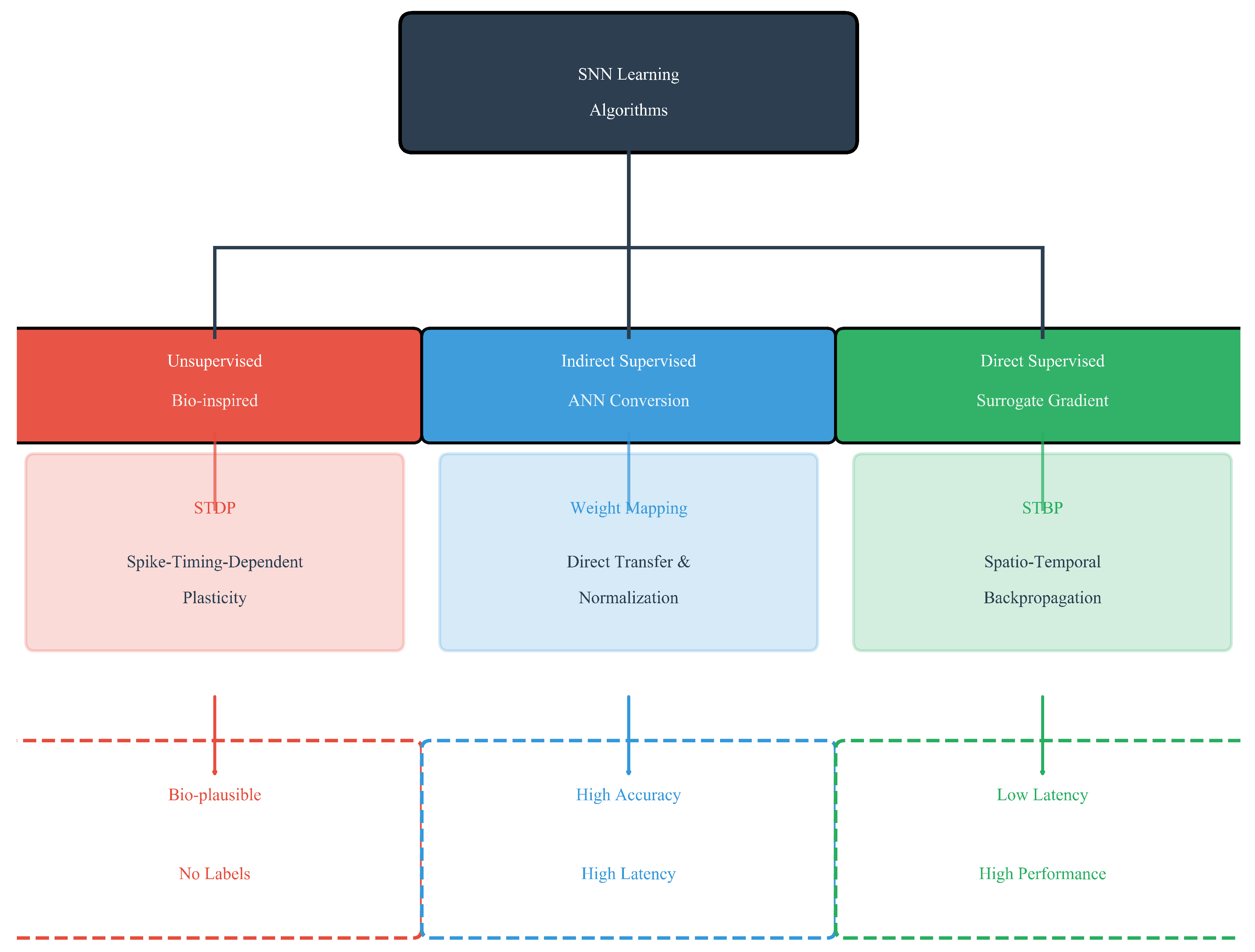
Figure 2.
SE-SNN Overall Architecture for DVS-CIFAR10 Classification.
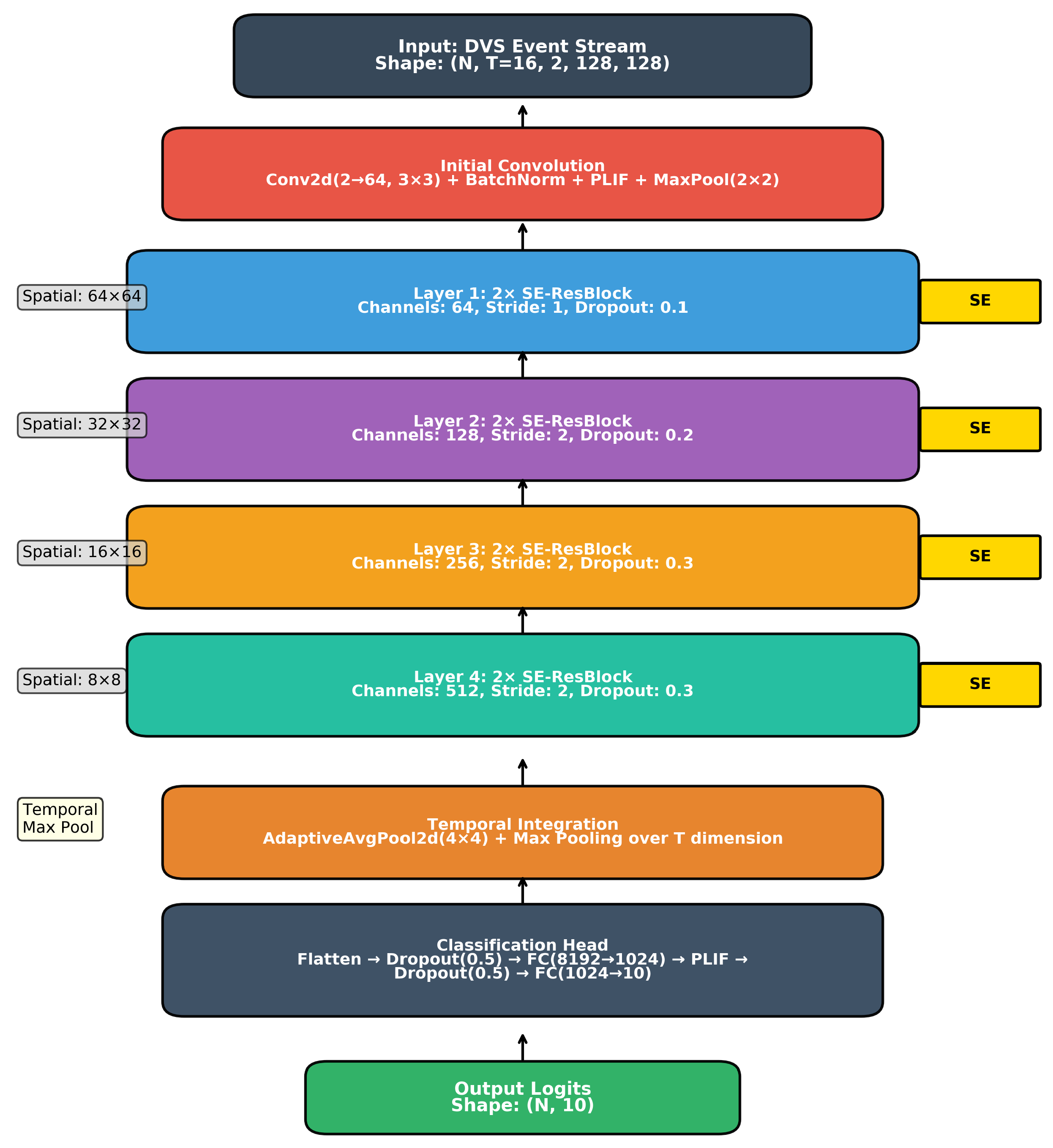
Figure 3.
Evolution of learnable parameters across different layers during training. (a) Time constant convergence. (b) Firing threshold convergence.
Figure 3.
Evolution of learnable parameters across different layers during training. (a) Time constant convergence. (b) Firing threshold convergence.
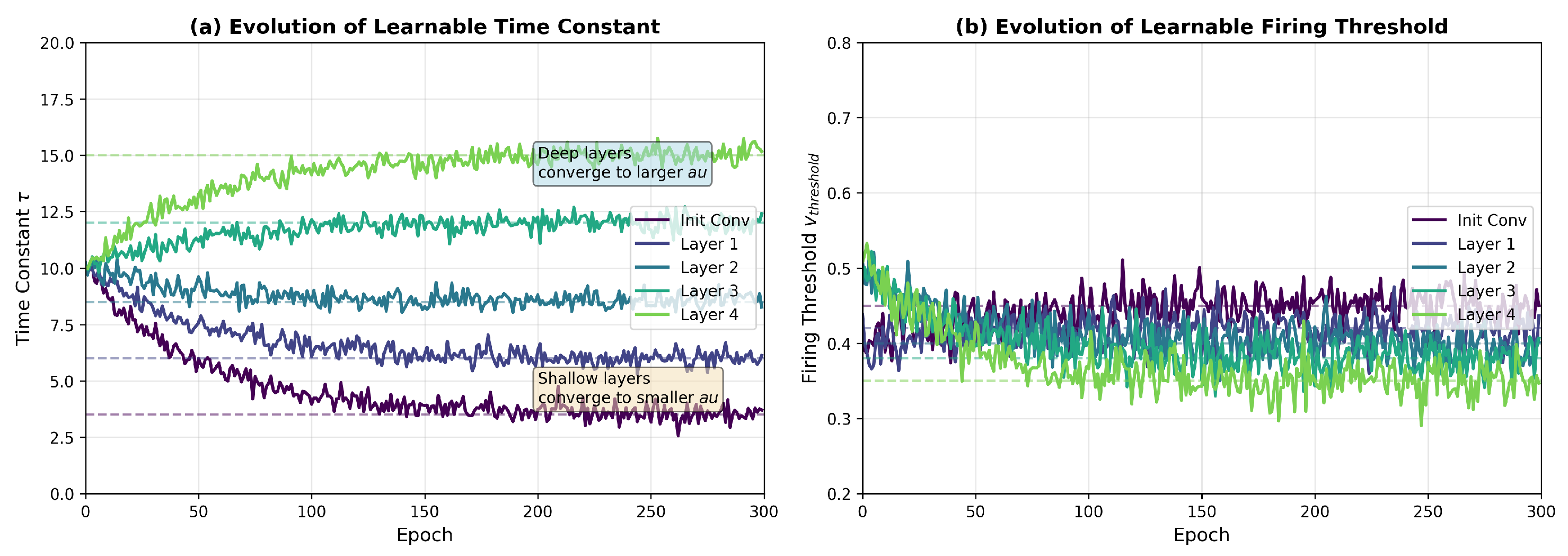
Figure 4.
Average firing rates across different layers and timesteps. Lower layers exhibit higher activity due to rich edge information in event data.
Figure 4.
Average firing rates across different layers and timesteps. Lower layers exhibit higher activity due to rich edge information in event data.
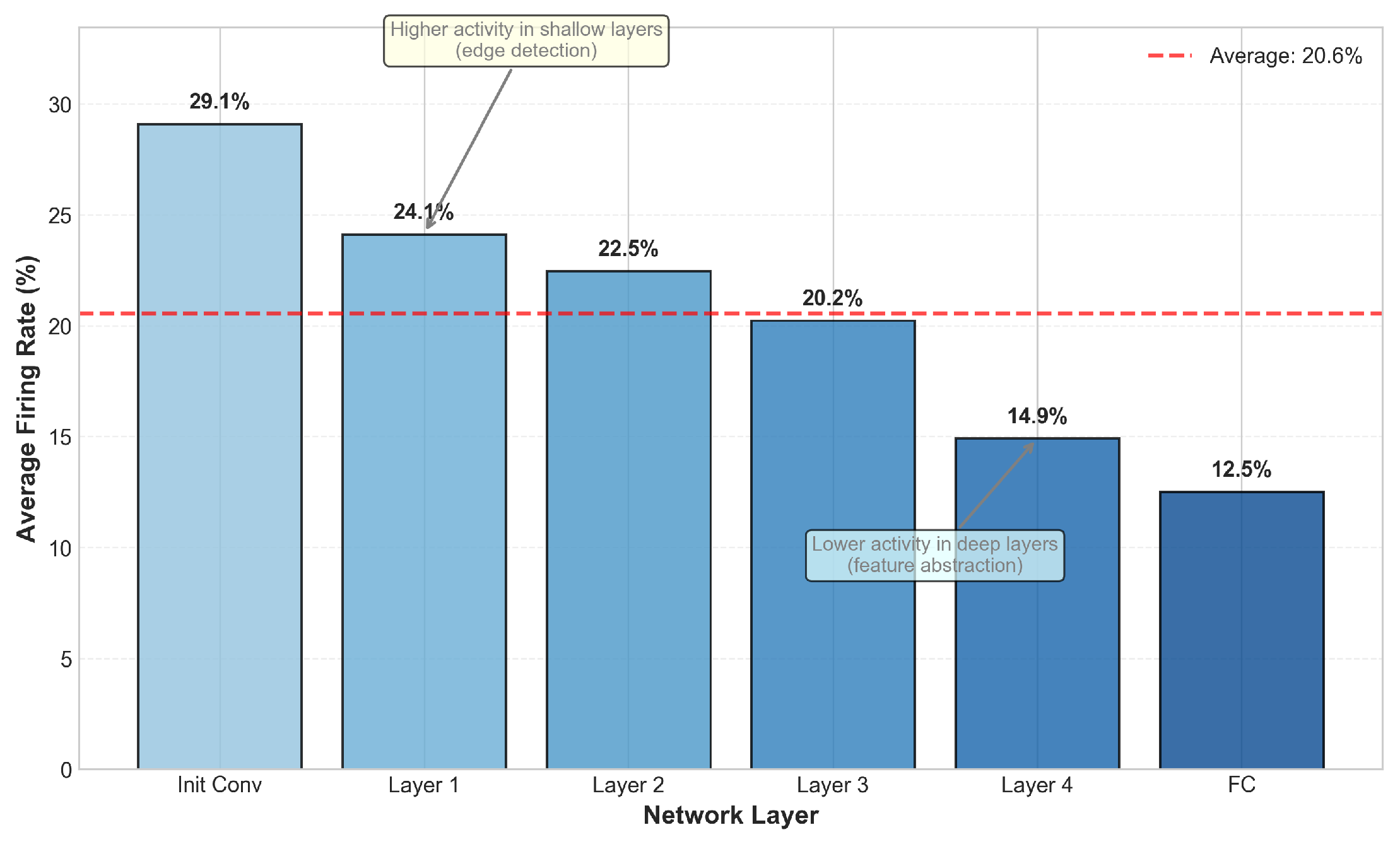
Table 1.
Comparison of Neural Encoding Schemes in SNNs.
| Encoding Scheme | Temporal Precision | Energy Efficiency | Noise Robustness | Primary Applications |
|---|---|---|---|---|
| Rate Coding [25] | Low | Low | High | Static image classification, ANN conversion |
| TTFS/Latency Coding [26] | High | High | Medium | Real-time processing, event-based vision |
| Rank-Order Coding [27] | High | High | High | Rapid categorization, olfaction |
| Phase Coding [28] | High | Medium | Medium | Navigation, temporal pattern recognition |
| Encoding [29] | Medium | High | High | Biomedical signals, wearable devices |
Table 2.
Comparison of SNN Learning Algorithms.
| Learning Paradigm | Supervision | Latency | Accuracy | Biological Plausibility |
|---|---|---|---|---|
| STDP [42] | Unsupervised | Low | Low | High |
| ANN-to-SNN Conversion [43] | Supervised | Very High | Very High | Low |
| Surrogate Gradient (BPTT) [41] | Supervised | Low | High | Medium |
| Hybrid (Conversion + Fine-tuning) [44] | Supervised | Medium | Very High | Medium |
| Local Supervised Learning [45] | Supervised | Low | Medium | High |
Table 3.
Detailed Architecture Configuration of SE-SNN.
| Stage | Layer | Configuration | Output Size | Stride | SE | Params |
|---|---|---|---|---|---|---|
| Input | - | DVS event frames | - | - | - | |
| Stem | Conv | , 64 | 1 | No | 1,152 | |
| BN | - | - | - | - | 128 | |
| PLIF | - | - | - | 2 | ||
| MaxPool | 2 | - | - | |||
| Layer1 | SE-ResBlock | 1 | Yes | 74,240 | ||
| SE-ResBlock | 1 | Yes | 74,240 | |||
| Layer2 | SE-ResBlock | 2 | Yes | 262,784 | ||
| SE-ResBlock | 1 | Yes | 262,784 | |||
| Layer3 | SE-ResBlock | 2 | Yes | 1,049,088 | ||
| SE-ResBlock | 1 | Yes | 1,049,088 | |||
| Layer4 | SE-ResBlock | 2 | Yes | 4,195,840 | ||
| SE-ResBlock | 1 | Yes | 4,195,840 | |||
| Neck | AdaptiveAvgPool | - | - | - | ||
| TemporalMax | max over T | - | - | - | ||
| Head | Flatten | - | - | - | - | |
| Dropout | - | - | - | - | ||
| FC + PLIF | - | - | 8,389,632 | |||
| Dropout | - | - | - | - | ||
| FC | - | - | 10,250 | |||
| Total Parameters | 19,566,066 | |||||
Table 4.
Comparison with state-of-the-art methods on CIFAR10-DVS.
| Method | Type | Architecture | Timestep | Accuracy (%) | Params (M) |
|---|---|---|---|---|---|
| STBP-tdBN [34] | Direct | ResNet-19 | 10 | 67.8 | 12.6 |
| PLIF [46] | Direct | PLIF-Net | 20 | 74.8 | 11.3 |
| SEW ResNet [32] | Direct | Wide-7B-Net | 16 | 74.4 | 15.8 |
| SE-PLIF-SNN (Ours) | Direct | SE-ResNet | 16 | 78.8±0.2 | 19.6 |
| SE-PLIF-SNN (Ours) | Direct | SE-ResNet | 10 | 76.5 ± 0.3 | 19.6 |
Disclaimer/Publisher’s Note: The statements, opinions and data contained in all publications are solely those of the individual author(s) and contributor(s) and not of MDPI and/or the editor(s). MDPI and/or the editor(s) disclaim responsibility for any injury to people or property resulting from any ideas, methods, instructions or products referred to in the content. |
© 2026 by the authors. Licensee MDPI, Basel, Switzerland. This article is an open access article distributed under the terms and conditions of the Creative Commons Attribution (CC BY) license (http://creativecommons.org/licenses/by/4.0/).
Copyright: This open access article is published under a Creative Commons CC BY 4.0 license, which permit the free download, distribution, and reuse, provided that the author and preprint are cited in any reuse.


