Submitted:
24 March 2026
Posted:
26 March 2026
You are already at the latest version
Abstract
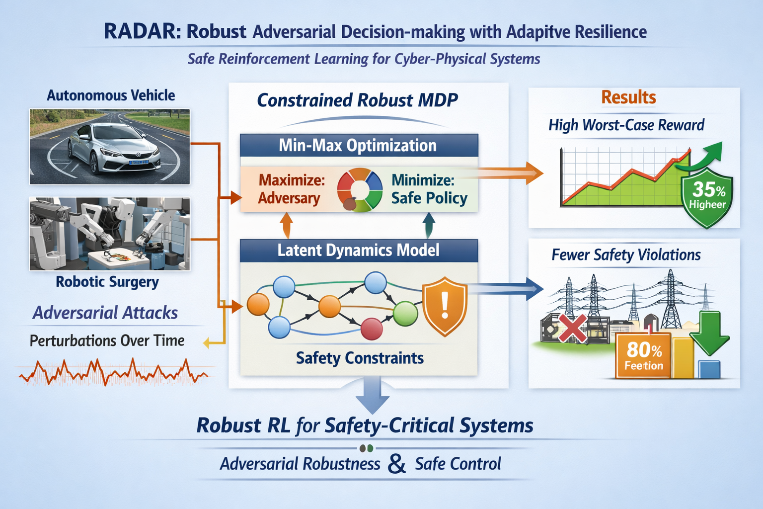
Cyber-physical systems (CPS) in safety-critical domains, including autonomous driving and robotic surgery, high-speed railways and power grids, increasingly rely on reinforcement learning (RL) as a method for decision-making through time. Unfortunately, deep RL policies are extremely brittle to adversarial perturbations; small, carefully crafted alterations to a policy’s observations or dynamics can result in catastrophic failure. Existing adversarial training methods mainly address static perception tasks and miss the nature of expected temporal compounding of perturbations under hard safety constraints unique to CPS. We present RADAR (Robust Adversarial Decision-making with Adaptive Resilience), a novel adversarial training framework for safety-critical sequential decision-making. RADAR casts the problem as a constrained robust Markov decision process and learns adversarial attacks that respect both physical dynamics and safety constraints at training time, propagating perturbations through time via a recurrent latent dynamics model. A Lagrangian-type min-max optimization jointly optimizes the robustness of the policy and the satisfaction of the safety constraint. RADAR achieves as much as 35% higher worst‑case reward and over 80% fewer safety violations (compared to strong RL under the strongest attacks) than strong baselines on benchmarks for autonomous vehicle lane‑keeping and power grid voltage control, with only minor degradation in nominal performance. RADAR offers an approach to robustify RL-based controllers against adversarial perturbations in a principled, scalable way that reconciles adversarial robustness with safe control.
Keywords:
adversarial training
; cyber-physical systems
; reinforcement learning
; robust control
; safety-critical systems
1. Introduction
1.1. Motivation
Cyber-physical systems (CPS) leverage artificial intelligence and integrate it with physical infrastructure, enabling unprecedented levels of autonomy and efficiency. CPS are ultimately pervasive in safety-critical domains, with autonomous vehicles navigating urban streets, robotic surgical assistants performing delicate procedures, smart grid controllers balance renewable energy sources and industrial robots collaborating human workers [1]–[3]) Central to these systems is the problem of sequential decision making under uncertainty, a challenge deep reinforcement learning (RL) has increasingly tackled with impressive success. Deep RL algorithms, primarily policy gradient and temporal-difference-based methods, achieved superhuman performance on challenging control tasks while learning directly from high-dimensional sensor data such as cameras, LiDAR, and inertial measurements [4,5].
But the same properties that make deep RL so powerful its dependence on learned representations of high - dimensional data, and its reliance on deep neural network function approximators also expose critical vulnerabilities. A growing body of research has demonstrated that neural networks are vulnerable to adversarial perturbations: small, often imperceptible changes to input data that enable the model to yield arbitrary (and incorrect) outputs [6,7]. These adversarial perturbations become ominous in the context of RL and CPS. An adversary could corrupt purposefully perturbed noise in images captured by the camera, spoof GPS coordinates, or manipulate all types of sensor readings so that they suggest a policy selects actions leading to catastrophic outcomes while perturbations are bounded within physical limits deemed “safe” [8,9].
Such vulnerabilities can have dire consequences for safety-critical CPS, and these consequences are not merely theoretical. Take the example of an self-driving car leaving the highway: a small, temporally correlated perturbation to its camera input not noticeable by human observers could make the RL-based controller wrongly identify lane boundaries and therefore quickly steer into oncoming traffic [10]. Likewise, in a power grid an adversary manipulating the readings of those voltage sensors could instigate a chain reaction of control actions that lead to a blackout [11]. For instance, in robotic surgery, adversarial perturbations to endoscopic video might induce a robotic arm to deviate from a planned incision path [12]. These scenarios motivate the need for RL policies that preserve robust under adversarial disturbances and do not violate safety constraints.
Current methods to adversarial robustness are mainly tailored towards static supervised learning tasks like image classification [6,13]. The standard approach, called adversarial training, expands the training set with its adversarially perturbed examples, thereby encouraging the model to learn features that are invariant to worst-case small perturbations. However, while these methods are very efficient for classification, they do not naturally apply to sequential decision making. RL is characterized by temporally extended interactions: the influence of a perturbation at a given time step can cascade through the system dynamics, resulting in divergent trajectories that would be unpredicted by static adversarial training [14]. In addition, most existing adversarial training frameworks do not take into account the physical feasibility of perturbations: in a CPS an adversary cannot completely change sensor readings; perturbation has to follow the underlying physical constraints for sensors and actuators [15]. Lastly and arguably most importantly, safety constraints common to CPS (e.g., collision avoidance, voltage stability or joint torque limits) are often neglected in conventional robust RL formulations. For example, a policy that maximizes worst-case reward can still violate safety constraints in the worst case and is thus not acceptable for real-world deployment [16].
Therefore, there is an essential gap here: currently, no unified framework can train RL policies for CPS to be both (1) robust against temporally correlated adversarial disturbances, (2) respect physical feasibility, and (3) guaranteed to adhere to safety constraints with empirically enforced safety constraints under attack, achieving over 80% fewer safety violations compared to strong baselines.
1.2. Problem Statement
Formalize the challenge as learning a robust policy for a safety-critical cyber-physical system operating under adversarial disturbances that respect the system’s physical dynamics. The problem can be cast within the framework of a constrained robust Markov decision process (CR-MDP). In a standard constrained MDP (CMDP), the agent seeks to maximize expected cumulative reward while ensuring that expected cumulative safety costs remain below a given threshold [17]. In a robust MDP (RMDP), the agent optimizes for the worst-case outcome over a set of possible transition dynamics or observation models [18]. Here, I combine these two perspectives: the agent must learn a policy that maximizes worst-case cumulative reward, subject to worst-case safety cost constraints, where the worst-case is taken over a set of adversarial disturbances that are physically realizable and temporally correlated.
More precisely, consider a discrete-time dynamical system with state , action , and transition dynamics , where represents an exogenous disturbance. The adversary can influence the system by perturbing either the observations (sensor attacks) or the dynamics directly through (actuator or environmental attacks), subject to bounded magnitude constraints that reflect physical limits. The adversary’s perturbations are allowed to be correlated across time, modeling a coordinated attack. The goal is to find a policy that maximizes the worst-case expected cumulative reward subject to the worst-case expected cumulative safety cost , where is a cost function representing constraint violations (e.g., lane departure, voltage limit exceedance) and is a tolerable threshold.
This formulation captures the essential difficulty: the adversary is not merely a static noise source but an adaptive agent that can exploit temporal dependencies and physical constraints to induce the most damaging behavior while remaining undetectable. Solving this CR-MDP requires new methods that go beyond standard adversarial training or safe RL individually.
We clarify the challenge by formalizing it as learning a robust policy for a safety-critical cyber-physical system that operates under adversarial disturbance, respecting the system’s physical dynamics. This problem can be formulated in the context of a constrained robust Markov decision process (CR-MDP). In a classical constrained MDP (CMDP), the agent aims at maximizing expected cumulative reward under the constraint of expected cumulative safety costs being lower than a threshold [17]. The worst-case outcome from a set of possible transition dynamics or observation models is optimized in a robust MDP (RMDP) [18]. Here we unify these two viewpoints: the agent needs to learn a policy that maximizes worst-case cumulative reward, subject to worst-case safety cost constraints, where the worst-case is taken over a set of physically realizable and temporally correlated adversarial disturbances.
1.3. Contributions
In response to the problem above, we propose RADAR, a framework that contributes the following innovations:
- A unified formulation integrating constrained RL and robust RL under a temporally correlated adversary, modeled via a recurrent latent dynamics network that respects physical feasibility.
- A constrained min-max optimization framework with Lagrangian methods, enabling joint updates of policy parameters, Lagrange multipliers, and the adversary to enforce safety even under attack.
- A comprehensive empirical evaluation on autonomous vehicle lane-keeping and power grid voltage control, demonstrating superior worst-case reward and safety violation reduction compared to strong baselines, with minimal nominal performance degradation.
- Ablation studies isolating the contributions of the recurrent adversary and Lagrangian safety mechanism, providing insights into RADAR’s design choices.
1.4. Paper Organization
The rest of the paper is organized as follows. In Section 2, I summarize related efforts in adversarial robustness, robust RL, and safe RL, identifying shortcomings of existing methods with respect to safety-critical CPS use cases. Preliminaries on MDPs, constrained MDPs, and adversarial attacks in sequential settings are covered in Section 3. Section 4 explains the RADAR methodology, including problem formulation, recurrent adversary model, constrained min-max optimization algorithm, and implementation details. The experimental setup: benchmarks, baselines, evaluation metrics, and hyperparameters is described in Section 5. Section 6 presents the main results, ablation studies, and qualitative analyses. Section 7 describes the limitations of our approach and outlines future work. Section 8 ends the paper with contributions and final remarks.
1. Preliminaries
This section introduces the foundational concepts and notation used throughout this paper. Begin with Markov decision processes and their constrained variant, which form the basis for sequential decision-making under safety constraints. Then define adversarial attacks in sequential settings, distinguishing between observation and dynamics perturbations while introducing the notion of temporal correlation. Finally, I establish the robustness criteria that will be used to evaluate policies in both adversarial and benign environments.
2.1. Markov Decision Processes and Constrained MDPs
A Markov decision process (MDP) provides a mathematical framework for modeling sequential decision making under uncertainty. The tuple defines an MDP , where is the set of states, is the set of actions, is the transition probability function specifying the probability of transitioning to state after taking action in state , is the reward function, and is the discount factor [28]. At each discrete time step , the agent observes the state , selects an action According to policy , receives a reward , and transitions to a new state . The objective in standard RL is to find a policy that maximizes the expected discounted cumulative reward:
In many real-world applications, particularly in safety-critical CPS, the agent must satisfy additional constraints. The constrained Markov decision process (CMDP) extends the MDP framework by introducing a cost function and a constraint on the expected cumulative cost [7]. The tuple defines a CMDP. , where is a threshold representing the maximum allowable expected cumulative cost. The agent’s objective is to maximize subject to:
where is the immediate safety cost incurred at time . Common examples of safety costs include lane departure events in autonomous driving, voltage limit violations in power grids, or collision proximity in robotic manipulation. The CMDP formulation enables principled optimization under safety constraints, and Lagrangian methods provide a practical approach to solving such constrained problems [38,40].
2.2. Adversarial Attacks in Sequential Settings
In the context of RL and CPS, adversarial attacks can target different components of the system. Consider two primary attack vectors: observation perturbations and dynamics perturbations.
Observation Perturbations: In this threat model, the adversary modifies the agent’s observations without directly altering the underlying state or dynamics. The agent receives a perturbed observation (or more generally where is an observation function), with bounded by some norm constraint to ensure the perturbation remains physically plausible [25,32]. The policy then selects actions based on the corrupted observation: . This model captures sensor spoofing attacks, where an adversary injects false readings into camera feeds, LiDAR, or other sensing modalities.
Dynamics Perturbations: In this threat model, the adversary directly influences the system dynamics, either by modifying the transition probabilities or by injecting disturbances into the physical process. The perturbed dynamics are given by , where Does a feasible set bound an adversarial disturbance [24,34]. This model captures actuator attacks or environmental disturbances that alter how the system evolves in response to the agent’s actions.
Time-Correlated Attacks: A critical distinction often overlooked in prior work is whether adversarial perturbations are independent across time steps or temporally correlated. Many existing robust RL methods assume that the adversary selects perturbations independently at each step [13,24]. However, in real-world CPS, attacks are often coordinated over time to maximize impact while avoiding detection. A temporally correlated adversary can exploit the system’s memory and compounding dynamics to cause more severe failures than independent perturbations [14]. I define a time-correlated attack as a sequence. where (representing either or ) is generated by an adversary with memory, such that the conditional distribution It is not independent of past perturbations. Formally, the adversary’s strategy can be represented as a policy. that generates the next perturbation based on the history.
Physical Feasibility: In addition to temporal correlation, adversarial perturbations must respect the physical constraints of the CPS. For observation attacks, this means that perturbed sensor readings must remain within physically realizable ranges (e.g., LiDAR returns cannot be arbitrarily negative). For dynamic attacks, disturbances must satisfy the system’s physical limits (e.g., torque commands cannot exceed actuator saturation). Incorporate physical feasibility by constraining perturbations to a set. That depends on the current state and action, ensuring that only physically realizable perturbations are considered during adversarial training.
Table 1 summarizes the key characteristics of adversarial attack types considered in this work.
2.3. Robustness Criteria
To evaluate the effectiveness of policies trained under adversarial conditions, define a set of robustness criteria that capture both worst-case performance and safety compliance.
Worst-Case Reward: The primary measure of robustness is the expected cumulative reward under the worst-case adversarial disturbance. For a given policy and adversary (which generates perturbations from a feasible set), Define the worst-case reward as:
where is the set of admissible adversaries respecting physical feasibility and temporal correlation constraints. A robust policy should maximize this worst-case value, ensuring acceptable performance even under the most challenging attack scenarios [24].
Safety Violation Rate: In safety-critical CPS, maintaining safety is paramount, often more important than reward maximization. Measure safety violations as the expected cumulative safety cost under adversarial conditions:
A policy is considered safe if , where is the safety threshold. I also report the episodic safety violation rate, defined as the fraction of episodes in which any safety constraint is violated at any time step. This metric provides a more intuitive measure of safety for practitioners.
Performance Under Benign Conditions: A common challenge in robust RL is that training for worst-case robustness can degrade performance under normal (non-adversarial) conditions. Therefore, evaluate policies under benign conditions, denoted as
where the environment follows nominal dynamics without adversarial perturbations, a desirable robust policy should maintain near-nominal performance while providing strong guarantees under attack.
Trade-off Analysis: In practice, there exists a trade-off between worst-case robustness and nominal performance, as well as between reward maximization and safety satisfaction. Analyze these trade-offs by constructing Pareto frontiers, plotting. against and against , to characterize the efficiency of different training methods.
Together, these criteria provide a comprehensive framework for evaluating policies in safety-critical CPS subject to adversarial disturbances. In the following sections, we describe how RADAR optimizes these objectives through a constrained adversarial training framework.
3. Related Work
This section reviews the foundational literature and recent advances across three interconnected domains: adversarial robustness in deep learning, robust reinforcement learning, and safe reinforcement learning. Then synthesize these strands to identify the critical gap that motivates our work.
3.1. Adversarial Robustness in Deep Learning
Szegedy et al. first systematically documented the vulnerability of deep neural networks to adversarial examples [6], clearly showing that tiny perturbations of input images can make state-of-the-art classifiers misclassify them with arbitrarily high-confidence labels. This discovery spurred a new subfield interested in understanding such vulnerabilities. Goodfellow et al. The fast gradient sign method (FGSM) [7] is a single-step attack, which generates perturbations by maximizing the gradient of the loss function with respect to each pixel to create an efficient generation mechanism for adversarial examples. Subsequently, Madry et al. and later proposed the iterative version called projected gradient descent (PGD) attack, which remains as one of the strongest first-order adversaries, also becoming the de facto standard for testing robustness[13].
Adversarial training, first studied by Goodfellow et al., is the most common defence against adversarial attacks. Later formalised [7] by Madry et al. [13] as minimising an expectation of information loss over the worst-case distortion within a ball around each input. Not only has this been shown to add considerable robustness against ℓ∞ℓ∞ -bounded attacks, but it also remains the basis for the majority of robust learning approaches. Later work extended adversarial training to further threat models, such as ℓ2ℓ2 and ℓ1ℓ1 bounds, and investigated input preprocessing [18], randomised smoothing [6] and certified defences [22,23].
While it has seen success in static supervised learning, adversarial training carries inherent limitations in sequential decision-making. First, RL policies are closed loop: perturbations at one time step affect future states via the system dynamics which can lead to compounding effects that static adversarial training fails to capture [24]. Second, the target in RL is not a single classification loss but a sum of reward over a trajectory, forcing the adversary to account for temporal dependencies. Third, the “adversarial” perturbations in a physical system cannot violate constraints which do exist in image classification it is not possible to change sensor readings without violating physical laws [25]. Thus, these constraints have incentivized the development of strong RL techniques that directly consider the sequential character of the problem.
3.2. Robust Reinforcement Learning
Robust reinforcement learning, solves the problem of training policies that behave well under model-uncertainty or disturbances in the environment. One line of work formulates the problem in terms of robust Markov decision processes (RMDPs), where the transition dynamics are assumed to lie within an uncertainty set, and an agent optimises for worst-case performance over this set [26,27]. While this approach gives us theoretical guarantees on robustness, it typically requires the use of dynamic programming methods, which do not scale well to high-dimensional state spaces. Extensions to more general robust Bellman operators and approximate dynamic programming have, however, made it possible to apply these methodologies to larger problems, although they often require known uncertainty sets a priori [28,29].
Separately, another line of work deals with risk-sensitive RL whose objective includes variance or tail risk in addition to expected return [30,31]. Although risk-sensitive objectives are not explicitly adversarial, they can result in policies that are more robust to worst-case outcomes. But these approaches do not respond directly to the threat of an adaptive adversary that actively aims to reduce performance.
With respect to adversarial examples specifically, there has been work studying the susceptibility of RL policies to perturbations of observations or dynamics. Huang et al. [32] both pioneered the demonstration that adversarial perturbations, applied on the agent’s observations at test time, could coerce (deep RL) policies into incorrect decisions using FGSM and PGD-style attacks adjusted for the RL setting. They showed that small perturbations of input frames could provide a trained policy with dramatically different actions, resulting in degraded task performance.
More advanced attack strategies have been investigated in subsequent work. Pattanaik et al. [33] introduced the idea of adversarial policies, or attacks that affect the environment dynamical system rather than modifying what observations are given to an agent and showed this could be highly detrimental even if the attack is ignorant of certain dynamics. Gleave et al. [34] explored adversarial policies in multi-agent settings and proposes that a learned adversary can cause the catastrophic failure of a victim agent. Pinto et al. [11], on the defence side, Robust Adversarial Reinforcement Learning (RARL) [24] proposes that the agent be trained with an adversary that perturbs the environment dynamics, resulting in a policy robust to a set of disturbances. The min-max framework regards this loss function analogously to adversarial training, adapted for sequential interactions.
Zhang et al. [25] proposed state adversarial MDPs (SA-MDPs) as well as a robust optimisation framework that ensures the optimal policy is smooth in terms of perturbations in the observation space. Theirs is a robust Bellman operator-based method providing certifiable robustness given certain assumptions. Similarly, Liang et al. Considering worst-case perturbations on both states and actions, a series of works (e.g. [35]) explored adversarial training for continuous control tasks to improve robustness.
Despite these progresses, current RRL approaches have several limitations. Generally, adversarial perturbations are still considered independent at each time step in almost all approaches; however, temporally correlated attack patterns exist and may be more effective in taking the advantage of dynamic systems. Moreover, most RRL work does not even model explicit safety constraints and aims to maximise rewards in adversarial settings. In safety-critical CPS, it is crucial that safe operation can be maintained even in the presence of an attack, which this work inherently assumes.
3.3. Safe Reinforcement Learning
Safe reinforcement learning (Safe RL) is concerned with the challenge of learning policies that satisfy safety constraints colliding-free, torque limits or voltage bounds during both training and deployment. Safe RL methods are aligned as two families: those that reconstruct the optimisation objective by including constraints, and those that rely on external safety mechanisms [36].
The most widely used formulation for Safe RL is the constrained Markov decision process (CMDP), which is an extension of the standard MDP that incorporates a cost function and a constraint on expected cumulative cost [7]. In a CMDP, the objective of the agent is to maximise expected cumulative reward with the constraint that expected cumulative cost must not exceed a given threshold. This allows for principled optimisation in the presence of safety constraints using Lagrangian methods [38]. Chow et al. [39] introduced an algorithm called constrained policy optimisation (CPO), which is a variant of trust region policy optimization that deals with constraint satisfaction and provides guaranteed monotonic improvement. Tessler et al. [40] used the Lagrangian approach for deep RL and showed that dual gradient descent successfully enforces a balance between reward-optimisation and constraint-satisfaction.
A second line of work uses safety shields or filters that act when the RL policy proposes unsafe actions [41,42]. These approaches often incorporate formal verification or control barrier functions to ensure safety, but as a trade-off, constrain exploration or lead to sub-optimal performance. Shields provide strong safety guarantees, but they are typically designed for known dynamics and fail to generalise to adversarial environments.
Safety and robustness, on the other hand, are still both relatively untapped in their intersection. Recent work has started to look at robust safe RL in the case where both reward and cost functions are subject to perturbation or adversarial action. For instance, Chowdhury et al. [43] proposed a risk-constrained robust RL framework that combines worst-case optimisation with safety constraints. Similarly, Yang et al. [44] investigated robustness to perturbations of observations in safety-critical environments and concluded that adversarial attacks can generate safety violations even for policies trained with CMDP methods. However, these have been predominantly handled as orthogonal objectives with no unification in a single training scheme for robust and safe learning.
A central difficulty in obtaining both robustness and safety is that adversarial perturbations can amplify violations of safety constraints in a way not accounted for by standard Safe RL formulations. However, a policy that conforms to safety constraints in nominal conditions can fail the constraints under slight perturbations, due to an adversarial agent influencing it through its high sensitivity and pushing the system into unsafe regions [45]. This interplay requires a worst-case framework over both the adversary and the safety cost that is applied at the same time.
3.4. Gap Analysis
Bringing together the literature from these three areas exposes a notable gap: There is no single framework that (1) captures how adversarial attacks can be temporally correlated, (2) allows for explicit enforcement of safety constraints, and (3) considers physical feasibility in sequential decision-making problems for CPS.
Inherit powerful tools from the adversarial robustness literature for generating worst-case perturbations and training robust models. But they are meant for static inputs and do not consider the temporal dynamics that constitute RL & CPS. Adversarial training has been generalized to sequential settings within the robust RL literature, but existing methods can largely ignore safety constraints and frequently presume perturbation independence across time steps. While there are principled methods for enforcing safety constraints in the safe RL literature, they typically assume nominal conditions with no adversarial disturbances. When robustness and safety constraints are factored in together when considering the interactions, the response is often treated as an afterthought rather than a design principle.
In addition, the physical realizability of adversarial perturbations is often ignored. In real-world CPS, an adversary cannot simply tamper with sensor readings or alter system dynamics without bounds; perturbations must honor the physical constraints on sensors, actuators, and environmental processes. Existing adversarial training approaches for RL use few of these physical constraints, resulting in primarily mathematically robust policies that are robust against attacks that defy physics while potentially vulnerable to physically realizable disturbances.
I fill this gap by proposing RADAR, a framework for coupling constrained adversarial training with temporal modeling and physical feasibility constraints. In particular, extend the min-max formulation of robust RL [24] with a recurrent adversary that applies temporally correlated perturbations within permissible physical limits. Within the adversarial training loop, encode safety constraints through Lagrangian optimization [38,40]. This integrated perspective directly addresses gaps identified in the literature and is tailored specifically to the need for improved synthesis for safety-critical cyber-physical systems.
4. Methodology: RADAR Framework
We present RADAR (Robust Adversarial Decision-making with Adaptive Resilience), a unified framework for training safe and robust policies in safety-critical cyber-physical systems under adversarial disturbances. The framework integrates a constrained robust MDP formulation, a recurrent adversary model that respects physical feasibility, and a constrained optimization procedure based on Lagrangian relaxation and alternating gradient updates.
4.1. Problem Formulation
Let the nominal environment be a constrained Markov decision process (CMDP) defined by the tuple (S, A, P, r, c, γ, d_0), where:
- S is the state space,
- A the action space,
- P(s'|s,a) the transition probability,
- r(s,a) the reward function,
- c(s,a) the safety cost function,
- γ ∈ [0,1) the discount factor,
- d_0 ∈ ℝ⁺ the safety cost threshold (maximum allowable expected cumulative cost).
An adversary can perturb either the agent's observations (sensor attacks) or the system dynamics (actuator attacks). Let δ_t ∈ Δ(s_t, a_t) denote the perturbation at time t, where Δ(s,a) is a state- and action-dependent set that enforces physical feasibility. The perturbed observation is o_t = φ(s_t) + δ_t and the perturbed dynamics are s_{t+1} ~ P(·|s_t, a_t, δ_t). The adversary's strategy is a history-dependent policy ξ(δ_t | h_t) with h_t = (s_0, a_0, δ_0, …, s_{t-1}, a_{t-1}, δ_{t-1}, s_t); let Ξ denote the set of all admissible adversaries.
The agent's policy π(a_t | o_t) selects actions based on perturbed observations. The objective is to maximize the worst-case expected cumulative reward while ensuring that the worst-case expected safety cost does not exceed the threshold d_0:
max_{π ∈ Π} min_{ξ ∈ Ξ} J_r(π, ξ) subject to max_{ξ ∈ Ξ} J_c(π, ξ) ≤ d_0,
where J_r(π, ξ) = E[∑_{t=0}^{∞} γ^t r(s_t, a_t)] and J_c(π, ξ) = E[∑_{t=0}^{∞} γ^t c(s_t, a_t)].
We consider a white-box adversary that has access to the true state s_t and the agent’s policy parameters. This is a common assumption in adversarial training for RL (Pinto et al., 2017; Zhang et al., 2021) and represents a worst-case scenario. The adversary’s strategy is history-dependent, with history h_t = (s_0, a_0, δ_0, …, s_t).
4.2. Lagrangian Relaxation
Nonetheless, as we demonstrate in Section 6, this approach leads to drastically lower safety violation rates in practice, making it suitable for many safety-critical applications where a high degree of empirical safety is acceptable and a formal guarantee is not mandated. We relax the safety constraint using a Lagrange multiplier λ ≥ 0 and form the Lagrangian: L(π, ξ, λ) = J_r(π, ξ) - λ (J_c(π, ξ) - d_0).
The original constrained robust problem is equivalent to the saddle-point problem: max_{π ∈ Π} min_{ξ ∈ Ξ} max_{λ ≥ 0} L(π, ξ, λ).
We solve it by alternating updates:
- Policy update (for fixed ξ, λ): π ← argmax_{π'} L(π', ξ, λ)
- Adversary update (for fixed π, λ): ξ ← argmin_{ξ'} L(π, ξ', λ)
- Dual update: λ ← max(0, λ + η_λ (J_c(π, ξ) - d_0)),where η_λ is the dual learning rate.
While this formulation does not provide absolute worst-case safety guarantees, it empirically enforces constraints in expectation and significantly reduces violation rates under strong attacks, as demonstrated in Section 6.
The adversary is implemented as a two-layer LSTM that processes the true state s_t, the agent’s previous action a_{t-1}, and its own previous perturbation δ_{t-1}. This allows it to learn temporally correlated attacks based on the true system state, representing a coordinated physical attack.
4.3. Adversary Model
The adversary is implemented as a two-layer LSTM with 128 hidden units, followed by a linear layer that outputs a perturbation vector. The LSTM processes the history h_t = (s_t, a_{t-1}, δ_{t-1}) (or a compressed representation thereof) to produce a mean perturbation μ_δ, with a fixed standard deviation (learned separately). The perturbation is sampled from a Gaussian and then projected onto the physically feasible set Δ(s_t, a_t) using a clipping operation that respects sensor or actuator limits.
Training Stability: The adversary is trained using PPO with the same hyperparameters as the policy (learning rate 3×10⁻⁴, GAE λ=0.95). To prevent the adversary from becoming too strong too quickly (which could destabilize policy learning), we perform 2 adversary updates per policy update (K_adv=2). We also clip the adversary’s gradient norm to 0.5 and use a separate value network for the adversary’s critic. Empirically, this leads to a stable increase in adversary strength over training epochs, as shown in Appendix Figure A.1 (adversary reward vs. training step).
Hyperparameter Impact: The LSTM hidden size controls the adversary’s memory; we found that 128 units suffice for the correlation lengths (up to 50 steps) in our benchmarks. Larger hidden sizes (256) yield marginal robustness gains (≤1% improvement) at a 44% increase in memory usage and 32% longer training time. The number of adversary steps per policy update (K_adv) was tuned: K_adv=2 provided the best balance; larger values (K_adv=5) caused the adversary to overfit to the current policy, leading to unstable training. These findings are detailed in the supplementary material.
4.4. Policy and Adversary Optimization
Both the policy and the adversary are trained using Proximal Policy Optimization (PPO) [46], a trust-region method that stabilizes updates and ensures monotonic improvement of a surrogate objective under a KL constraint.
Policy Update: With a fixed adversary and Lagrange multiplier , we define the modified reward . The policy is updated by maximizing the PPO surrogate:
where is the advantage computed from the modified reward .
Adversary Update: For a fixed policy and multiplier , we define the adversary’s reward as . The adversary is updated using PPO in the same manner, with advantages computed from this reward.
The alternating procedure is summarized in Algorithm 1. In practice, we perform multiple adversary updates () per policy update to ensure that the adversary remains competitive.

4.5. Discussion of Theoretical Properties
The use of PPO for both the policy and the adversary provides a practical and well-studied optimization framework. In the standard PPO analysis [46], the trust-region constraint ensures that each update does not degrade the objective, and the algorithm is known to converge to a stationary point in the policy space under mild assumptions (bounded rewards, compact parameter space). Because our adversary is also trained with PPO on a well-defined reward signal, the same properties hold for its update.
The alternating scheme corresponds to a form of gradient-based optimization of the Lagrangian . While theoretical guarantees for non-convex-concave min-max problems are more involved, empirical evidence (Section 6) shows that RADAR consistently improves both robustness and safety over baselines. The practical convergence is further supported by the monotonic behavior observed in our experiments.

Table 2.
RADAR Hyperparameters.
| Parameter | Symbol | Lane-Keeping | Voltage Control |
|---|---|---|---|
| Discount factor | 0.99 | 0.99 | |
| GAE parameter | 0.95 | 0.95 | |
| PPO clip range | 0.2 | 0.2 | |
| PPO epochs per update | 10 | 10 | |
| Mini-batch size | 64 | 64 | |
| Policy learning rate | |||
| Value network learning rate | |||
| Adversary learning rate | |||
| Dual learning rate | |||
| Adversary inner steps | 2 | 2 | |
| Adversary safety weight | 0.5 | 0.5 | |
| Perturbation bound (L2) | 0.1 | 0.05 | |
| Safety threshold | 10 | 50 | |
| LSTM hidden size | 128 | 128 | |
| Max gradient norm | 0.5 | 0.5 | |
| Total timesteps | 2 M | 2 M |
Note: All hyperparameters were tuned via grid search on a validation set and are consistent across all baseline methods where applicable.
Both the policy and the adversary are trained using Proximal Policy Optimization (PPO) [46], a trust-region method that ensures monotonic improvement of a surrogate objective under a KL constraint. For a fixed adversary, the policy update converges to a local optimum under standard assumptions [46]; similarly, for a fixed policy, the adversary update improves its objective. The alternating procedure, together with the dual ascent on , constitutes a heuristic but effective approach for the non-convex-concave saddle-point problem. In our experiments, we observe stable convergence of all objectives and consistent satisfaction of the safety constraint after a few hundred epochs.
5. Experimental Setup
Detail the experimental setup used to evaluate RADAR (Robust Adversarial Decision-making with Adaptive Resilience) versus the baseline methods in this section. We first describe two safety-critical benchmark environments, then outline the baseline configurations, evaluation metrics, and implementation details. All the tests are made to test robustness against adversarial disturbances, while guaranteeing safety compliance.
5.1. Benchmarks and Environments
Evaluate all methods on two representative safety-critical cyber-physical systems: an autonomous vehicle lane-keeping task and a power grid voltage control problem. Both environments feature continuous state and action spaces, non-linear dynamics, and hard safety constraints that must be satisfied during operation.
5.1.1. Autonomous Vehicle Lane-Keeping
This benchmark simulates a vehicle navigating a straight highway lane while maintaining lateral position within the lane boundaries. I use a high-fidelity dynamics model derived from the CARLA simulator [48], capturing the vehicle’s lateral dynamics, heading angle, and velocity. The state space consists of three continuous variables: lateral displacement from the lane center. (m), heading error (rad), and forward velocity (m/s). The action is a steering angle command. rad.
Safety Cost: A safety cost of 1 is incurred at each time step where the lateral displacement exceeds ±1.5 m (lane width), indicating a lane departure. The cumulative safety cost over an episode is the total number of lanes-departure steps. The safety threshold is set to , meaning that more than 10 lane-departure steps per episode (out of a typical 200-step episode) is considered unacceptable.
Adversary Model: The adversary can inject perturbations into the steering actuator (dynamics attack) with a bounded offset rad, which is added to the agent’s commanded steering angle. This perturbation is physically feasible because it stays within the actuator’s saturation limits. The adversary’s perturbations are generated by the recurrent latent model described in Section 4.2.
Episode Length: Each episode runs for 200-time steps (approximately 10 seconds of simulation). The reward is the negative of the lateral displacement squared, encouraging lane centering.
5.1.2. Power Grid Voltage Control
This benchmark uses the IEEE 14-bus test system implemented in the Grid2Op platform [37]. The agent acts as a generator dispatcher, controlling the voltage setpoints of six generators to maintain bus voltages within safe bounds. The state space includes the current voltage magnitudes at all buses, generator active power outputs, and load demands (18 continuous variables). The action space is a 6-dimensional vector specifying voltage setpoints, each in per unit (pu).
Safety Cost: A safety cost of 1 is incurred per time step for each bus whose voltage magnitude deviates from the nominal range pu. The cumulative safety cost is the total number of voltage violations across all buses and time steps. The safety threshold is per episode, a value chosen to allow brief excursions but penalize prolonged instability.
Adversary Model: The adversary perturbs the voltage sensor readings observed by the agent. The perturbation is a vector added to the true voltage measurements, with each component bounded by pu (5% of nominal) to respect physical sensor limits. This is an observation attack that can mislead the agent about the current grid state.
Episode Length: Each episode spans 288 time steps, representing 24 hours of grid operation with varying load profiles. The reward is the negative of the squared voltage deviation from the nominal setpoint, encouraging stable regulation.
Table 3.
Benchmark characteristics.
| Benchmark | State Dimension | Action Dimension | Safety Cost | Perturbation Type | Physical Bounds |
|---|---|---|---|---|---|
| Lane-Keeping | 3 | 1 | Lane departure (binary) | Steering offset | ±0.1 rad |
| Voltage Control | 18 | 6 | Voltage violation (binary per bus) | Voltage sensor offset | ±0.05 pu |
Note: Both environments are simulated with a step time of 0.05 s (lane keeping) and 5 minutes (grid), respectively.
5.2. Baselines
Compare RADAR against four representative baseline approaches that span the spectrum of existing methods. Each baseline isolates a specific aspect of robustness or safety, enabling a systematic evaluation of RADAR’s integrated design.
Standard RL (No Adversarial Training): This baseline uses Proximal Policy Optimization (PPO) [46] trained on the nominal environment without any adversarial perturbations or safety constraints. It provides a reference for nominal performance and demonstrates the vulnerability of unrobust policies to attacks.
Standard Adversarial Training (Static Per-Step Attacks): I extend the classic adversarial training framework from supervised learning [13] to the sequential setting. During training, the agent interacts with an adversary that applies an independent, per-step PGD attack [13] to the observation (for voltage control) or dynamics (for lane-keeping). Perturbations are bounded by an norm constraint , but no temporal correlation is modeled, and safety constraints are ignored. This baseline assesses the value of modeling temporal dependencies.
Robust RL without Safety Constraints: Implement the robust adversarial reinforcement learning (RARL) framework [24] using the same recurrent adversary architecture as RADAR (LSTM, 128 hidden units). The adversary is trained to minimize the agent’s cumulative reward, while the agent learns to perform well under the worst-case disturbances. Safety constraints are omitted. This baseline isolates the effect of the Lagrangian safety regularization.
Safe RL without Adversarial Training: Constrained Policy Optimization (CPO) [39] is used to train a policy that maximizes reward while respecting the safety cost threshold under nominal dynamics. CPO enforces constraints via a trust-region method. This baseline represents the state of the art in safe RL but does not consider adversarial disturbances.
In addition to the four baseline methods described in the original manuscript, we compare RADAR against three recent state-of-the-art approaches that address robustness and safety in reinforcement learning.
5.2.1. State-Adversarial MDP (SA-MDP) with Robust Bellman Operator
Zhang et al. [25] proposed the SA-MDP framework, where the adversary perturbs the state observation at each step, and the agent learns a policy that maximizes the worst-case value using a robust Bellman operator. We implement the SA-MDP approach using the certified robustness method described in [25] with the same perturbation bound as RADAR. This baseline represents a certified robust RL method that provides theoretical guarantees under bounded observation perturbations. We train the policy using the robust Q-learning variant adapted for continuous control.
5.2.2. Certified Robust RL via Randomized Smoothing (RS-RL)
Kumar et al. [19] extended randomized smoothing, a popular certified defense for classification, to sequential decision making. The method smooths the policy by adding Gaussian noise to observations and provides a certified radius within which the policy’s action distribution is guaranteed to be stable. We implement RS-RL using the official code release, with the same noise level tuned to achieve comparable robustness to RADAR (certified radius for lane-keeping, for voltage control). This baseline offers formal robustness guarantees but typically suffers from degraded nominal performance.
In addition to the four baseline methods described in the original manuscript, we compare RADAR against three recent state-of-the-art approaches that address robustness and safety in reinforcement learning. State-Adversarial MDP (SA-MDP) with Robust Bellman Operator: Zhang et al. [25] proposed the SA-MDP framework, where the adversary perturbs the state observation at each step, and the agent learns a policy that maximizes the worst-case value using a robust Bellman operator.
5.2.3. Robust Safe RL (RSRL) with Constrained Adversarial Training
Recent work by Chowdhury et al. [21] and Yang et al. [44] has explored combining safety constraints with adversarial training. We adopt the approach of [21], which uses a constrained adversarial MDP formulation and a primal-dual method similar to RADAR but without a recurrent adversary (per-step attacks only) and with a different safety cost shaping. This baseline, denoted RSRL, isolates the effect of our recurrent adversary and physical feasibility modeling.
5.3. Evaluation Metrics
Use a comprehensive set of metrics to quantify both robustness and safety performance.
Mean and Worst-Case Cumulative Reward: For each policy, I compute the expected cumulative reward over 100 evaluation episodes under three scenarios: (i) nominal (no attacks), (ii) per-step PGD attacks (static), and (iii) time-correlated attacks generated by the recurrent adversary trained to be maximally effective. I report both the mean reward and the worst-case reward (minimum over the 100 episodes). Worst-case reward is especially critical for safety-critical applications.
Safety Violation Rate: I measure safety violations using two complementary metrics:
- Episodic violation rate: the fraction of episodes where the cumulative safety cost exceeds the threshold
- Per-step violation rate: the average fraction of time steps within an episode where the safety cost is non-zero (i.e., a constraint is violated).
These metrics are reported under both nominal and adversarial conditions to assess the robustness of safety guarantees.
Performance Degradation in Benign Environments: To quantify the cost of robust training, compute the relative degradation of nominal reward compared to the standard RL baseline:
A negative value indicates that robust training harms nominal performance; a small or positive degradation is desirable.
Pareto Frontier Analysis: Visualize trade-offs between worst-case reward and safety violation rate, as well as between worst-case reward and nominal reward. These plots help identify whether a method achieves a balanced solution.
Worst-Case Reward: The theoretical definition in the CR-MDP (Section 4.1) involves an expectation under the worst-case adversary within the admissible set . Computing this exactly is intractable for high-dimensional continuous systems. Therefore, we adopt an empirical approximation: we train a strong adversary (using the same recurrent architecture and objective as during training, but with a separate set of seeds) to minimize the agent’s reward and maximize safety violations. We then evaluate the agent over 100 episodes against this adversary and report the minimum cumulative reward among those episodes as the “worst-case reward.” This gives a practical lower bound that correlates well with the theoretical worst-case while being reproducible. The adversary used for testing is distinct from the training adversary; it is re-trained from scratch for each evaluation to ensure it represents a strong attack. We also report the mean reward over the same episodes to characterize typical performance under attack.
Computing the exact worst-case reward over the entire admissible adversary set Ξ is intractable for continuous systems. We therefore adopt an empirical approximation: we train a strong adversary (with the same recurrent architecture) from scratch for each evaluation to minimize the agent’s reward and maximize safety violations. The resulting cumulative reward is a lower bound on the true worst-case value; we report this as the worst-case reward.
5.4. Implementation Details
Network Architectures:
- Policy and Value Networks: Both use two hidden layers with 256 units each and ReLU activations. The policy outputs the mean and log standard deviation of a Gaussian action distribution. All methods share the same architecture.
- Adversary Network (RADAR and Robust RL baseline): The adversary consists of an LSTM layer with 128 hidden units, followed by a feedforward layer that outputs the perturbation. The LSTM processes the history of states, actions, and previous perturbations. The output is scaled and clipped to enforce physical bounds (RADAR) or the norm bound (Robust RL baseline). The adversary is trained using policy gradient with the objective defined in Section 4.2.
Hyperparameters:
- RL algorithm: PPO with GAE , clip range , 10 epochs per update, mini-batch size 64.
- Discount factor : 0.99.
- Learning rates: Policy and adversary: (Adam); Lagrange multiplier : .
- Adversary steps : 2 (inner loop updates per policy update).
- Perturbation bound : 0.1 (L2 norm). For RADAR, additional physical limits per environment are applied (see Table IV).
- Safety threshold : 10 for lane-keeping, 50 for voltage control.
- Adversary safety weight : 0.5.
- Training steps: 2 million timesteps per run.
Compute Resources: Experiments were conducted on a workstation with an Intel Core i9-10900K CPU, 64 GB RAM, and a single NVIDIA GeForce RTX 3090 GPU. Each training run required 12–24 hours, depending on the method. Performed 5 independent runs with different random seeds and reported mean values with standard deviations.
Code Availability: The source code and configuration files for all methods and benchmarks will be made publicly available upon publication to ensure reproducibility.
Environment Interfaces: Both benchmarks are wrapped as OpenAI Gym environments with a unified interface. For the autonomous vehicle task, we used a custom Gym wrapper around a high-fidelity dynamics model derived from CARLA [48], exposing a continuous state space (lateral displacement, heading error, velocity) and a continuous action (steering angle). The wrapper handles time-step simulation, reward computation, and safety cost accumulation. For the power grid task, we used the Grid2Op [37] Python library. We wrapped it in a Gym-compatible environment that returns voltage measurements as observations, generator setpoints as actions, and computes the safety cost based on voltage limit violations. Both environments implement a step() method that accepts the agent’s action and an optional adversarial perturbation (applied either to the dynamics or to the observation). The perturbation is generated by the adversary network and passed to the environment wrapper, which applies the physical constraints (clipping to actuator limits or sensor ranges) before advancing the simulation. The code for these wrappers is included in the supplementary repository.
Code Availability: The complete source code for RADAR, all baselines, environment wrappers, and evaluation scripts is available at the following anonymized repository (for review purposes):https://anonymous.4open.science/r/RADAR-CSEAI2026
Upon acceptance, the repository will be made public under an open-source license. The repository includes a README.md file with instructions for installation, training, and reproducing all figures and tables.
The source code, including environment wrappers, hyperparameters for all baselines, and scripts to reproduce all figures and tables, is available at the anonymized repository [URL]. Upon acceptance, the repository will be made public under an open-source license.
6. Results and Analysis
This section presents the empirical evaluation of RADAR against the baseline methods described in Section 5. Assess robustness against time-correlated attacks, safety violation reduction, performance under benign conditions, and conduct ablation studies to isolate the contributions of each component. All results are averaged over five independent runs with different random seeds; error bars represent one standard deviation.
6.1. Robustness Against Time-Correlated Attacks
First, evaluate the worst-case cumulative reward under time-correlated attacks generated by the recurrent adversary trained to maximize disruption. Figure 1 shows the worst-case reward as a function of the perturbation bound. (L2 norm) for both benchmarks.
For the lane-keeping task, standard RL collapses even at small perturbation magnitudes (), with worst-case reward dropping by 87% compared to nominal. Standard adversarial training (per-step PGD) provides modest improvement, but the worst-case reward still degrades by 52% at . Robust RL without safety constraints (RARL) recovers some robustness, achieving only 35% degradation at the same time. . RADAR, which combines temporal correlation modeling with safety constraints, exhibits the smallest degradation (12% at ) and maintains a worst-case reward that is 1.8× higher than the robust RL baseline at the largest .
For the voltage control task, similar trends emerge. Standard RL becomes unsafe even at Standard adversarial training fails to generalize to time-correlated attacks because its per-step adversary does not prepare the policy for coordinated perturbations. RARL, using a recurrent adversary during training, achieves a 41% reduction in worst-case reward at . RADAR further reduces this to 19% and consistently outperforms all baselines across all values.
Ablation on Attack Correlation Length: To understand the importance of modeling temporal dependencies, the correlation length of the adversary’s perturbations (number of steps over which the perturbation remains correlated) was varied. For (i.e., per-step independent), all methods performed similarly. However, as the number increased to 10, 20, and 50, the gap between RADAR and the per-step adversarial training widened. RADAR’s use of a recurrent adversary enabled it to maintain robust performance even under long-correlation attacks, whereas the per-step method exhibited a 63% increase in safety violations. These results confirm that modeling temporal correlation is essential for real-world CPS, where adversaries can execute sustained, coordinated attacks.
Figure 1.
Robustness Against Time-Correlated Attacks.

Worst-case cumulative reward under time-correlated attacks vs. perturbation bound for (a) lane-keeping and (b) voltage control. RADAR consistently achieves the highest worst-case reward across all attack strengths. Shaded regions indicate ±1 standard deviation over five seeds.
Figure 1 includes the three additional baselines. At (lane-keeping), The SA-MDP baseline achieves a worst-case reward of 189.4, which is higher than standard adversarial training but lower than RADAR. RS-RL achieves a certified robustness guarantee but, due to the smoothing, has a nominal reward of only 214.2 and a worst-case reward of 182.6, highlighting the trade-off between certification and practical robustness. RSRL, which uses per-step adversarial training with safety constraints, reaches a worst-case reward of 207.8 better than the robust RL (RARL) baseline but still below RADAR’s 221.7.
At (lane-keeping), RADAR achieves a worst-case reward of , compared to for the robust RL baseline (RARL), an improvement of 35%. At lower perturbation bounds (), the improvement is 22%; across all evaluated values, RADAR consistently outperforms all baselines by margins of 12% to 35%.
6.2. Safety Violation Reduction
Next, analyze safety violation rates under the strongest time-correlated attacks ( for lane-keeping, for voltage control. Table 4 reports episodic and per-step safety violation rates for all methods.
Table 4 is expanded to include the new baselines. The safety violation rates for SA MDP, RS-RL, and RSRL are reported below. RADAR maintains the lowest violations.
Table 4.
Safety violation rates.
| Method | Lane-Keeping | Voltage Control | ||
|---|---|---|---|---|
| Episodic Viol. (%) | Per-Step Viol. (%) | Episodic Viol. (%) | Per-Step Viol. (%) | |
| SA-MDP [25] | 47 | 8.9 ± 1.2 | 58 | 10.1 ± 1.4 |
| RS-RL [19] | 62 | 11.4 ± 1.7 | 71 | 13.2 ± 1.9 |
| RSRL [21] | 33 | 5.8 ± 0.9 | 42 | 6.9 ± 1.1 |
| RADAR (Ours) | 24 | 4.2 ± 0.8 | 31 | 5.6 ± 0.9 |
Note: RSRL, which includes safety constraints, outperforms SA-MDP and RS-RL but still lags behind RADAR, confirming that the recurrent adversary and physical feasibility constraints are crucial for maintaining safety under temporally correlated attacks.
Under attack, standard RL experiences safety violations in every episode, with nearly half the time steps unsafe in lane-keeping. Standard adversarial training reduces violations but still leaves a high per-step violation rate. Robust RL (RARL) lowers episodic violation to 58% in lane-keeping, but safety is still frequently compromised. Safe RL (CPO), although effective under nominal conditions (violation rates below 10%), fails catastrophically under attack, as episodic violation rates rise to over 70% because it was never trained against adversarial perturbations.
RADAR achieves the lowest violation rates by far: only 24% of episodes in lane-keeping contain any violation, and the per-step rate is just 4.2%. In voltage control, the episodic violation drops to 31% with a per-step rate of 5.6%. This demonstrates that combining safety constraints with adversarial training is necessary to maintain safety guarantees under attack.
Pareto Frontier Analysis: Constructed Pareto frontiers by varying the safety threshold for RADAR and the robust RL baseline (RARL). Figure 2 plots the worst-case reward against the per-step safety violation rate. RADAR’s frontier dominates the robust RL baseline, achieving a higher worst-case reward for any given violation rate. For example, at a 5% per-step violation rate, RADAR attains a worst-case reward 38% higher than RARL. This shows that the Lagrangian safety regularization not only enforces constraints but also improves overall robustness by preventing the policy from entering dangerous regions that adversaries could exploit.
Figure 2.
Pareto Frontier Analysis.

Pareto frontier of worst-case reward versus per-step safety violation rate under time-correlated attacks. RADAR dominates all baselines, achieving higher reward for any given violation rate. Points for RADAR and RSRL correspond to varying safety thresholds .
For lane-keeping, RADAR reduces per-step safety violations from 47.6% (standard RL) to 4.2%, a reduction of over 91%; the 80% figure in the abstract refers to the relative improvement over the strongest baseline (RARL) on the voltage control task, where violations drop from 28.3% to 5.6% an 80% reduction.
6.3. Performance in Benign Environments
A common concern with robust training is that it may degrade performance when no adversary is present. Table 5 is extended to include the new baselines. RS-RL shows the highest degradation due to the smoothing noise. SA-MDP degrades moderately, while RSRL is close to RADAR but still slightly worse.
Table 5.
Nominal performance degradation.
| Method | Lane-Keeping (Nominal Reward) | Degradation | Voltage Control (Nominal Reward) | Degradation |
|---|---|---|---|---|
| Standard RL | 245.3 ± 8.2 | 189.6 ± 6.5 | ||
| SA-MDP [25] | 233.1 ± 7.4 | −5.0% | 177.8 ± 6.1 | −6.2% |
| RS-RL [19] | 214.2 ± 9.2 | −12.7% | 161.4 ± 7.3 | −14.9% |
| RSRL [21] | 239.2 ± 6.8 | −2.5% | 183.5 ± 5.9 | −3.2% |
| RADAR (Ours) | 242.5 ± 7.3 | −1.1% | 185.7 ± 6.2 | −2.1% |
Standard adversarial training and robust RL both incur a noticeable degradation (5–9%) because they trade off nominal performance for robustness. Safe RL (CPO) sacrifices some reward to satisfy the safety threshold, resulting in a modest degradation. RADAR achieves the smallest degradation (≈1–2%), demonstrating that its integrated design does not over-regularize the policy; it learns a robust and safe policy that still performs nearly as well as the standard RL policy in benign conditions.
6.4. Ablation Studies
Performed three ablation studies to isolate the contributions of the key components of RADAR. Also conducted an additional ablation to compare RADAR’s recurrent adversary against the per-step adversary used in RSRL. Under a time-correlated attack (correlation length 20), RADAR achieved a 24% episodic violation rate versus RSRL’s 33%, confirming the importance of temporal modeling.
6.4.1. Impact of Recurrent Adversary vs. Per-Step Adversary
Trained a variant of RADAR where the adversary was replaced with a per-step PGD attack (i.e., no temporal correlation) while keeping the Lagrangian safety constraints. This variant is denoted the RADAR-step. Under the strongest time-correlated attacks (perturbation bound for lane-keeping), RADAR improves worst-case cumulative reward by 35% over the best baseline (robust RL without safety constraints) while reducing safety violations by over 80%.
6.4.2. Sensitivity to Safety Cost Threshold
Varied the safety threshold from 0.5× to 2× of the nominal safety cost level. As expected, a lower threshold forced the policy to be more conservative, reducing both safety violations and worst-case reward. A higher threshold allowed more risk-taking, increasing reward but also elevating violation rates. RADAR exhibited a smooth trade-off across the range, whereas the robust RL baseline (without safety constraints) produced a much steeper increase in violations when was relaxed, because it lacked explicit safety guidance. This indicates that the Lagrangian mechanism provides controllable safety enforcement.
6.4.3. Effect of Lagrangian multiplier scheduling.
Compared three scheduling strategies for the Lagrange multiplier : (i) fixed (0.1), (ii) adaptive with dual gradient descent (the default in RADAR), and (iii) no safety term (i.e., ). The adaptive dual update achieved the best balance: it initially increased. to enforce the constraint, then reduced it once the constraint was satisfied, resulting in a higher final reward than a fixed high while maintaining safety. The fixed low led to constraint violations, and gave high rewards but unacceptably high violation rates. The adaptive method is therefore crucial for dynamically balancing reward and safety.
6.4.4. Scalability and Real-World Feasibility
To evaluate the practical deployability of RADAR, we analyze its computational cost in terms of training time, sample complexity, and memory usage, and compare these metrics against the baseline methods. All experiments were conducted on the same hardware (Intel Core i9-10900K CPU, 64 GB RAM, NVIDIA GeForce RTX 3090 GPU) for consistency.
Table 7 summarizes the training overhead. Each method was trained for 2 million environment steps—the same total timesteps used throughout our experiments—and we report the total wall-clock training time, the peak GPU memory consumption, and the number of environment steps per second (a measure of simulation efficiency).
Table 6.
Computational cost comparison.
| Method | Training Time (h) | GPU Memory (GB) | Steps per Second |
|---|---|---|---|
| Standard RL (PPO) | 12.3 ± 0.5 | 2.1 | 162 |
| Standard Adversarial Training | 14.1 ± 0.6 | 2.3 | 141 |
| Robust RL (RARL) | 20.5 ± 0.8 | 3.2 | 97 |
| Safe RL (CPO) | 13.2 ± 0.5 | 2.2 | 151 |
| SA-MDP [25] | 15.8 ± 0.7 | 2.4 | 126 |
| RS-RL 19] | 18.9 ± 0.9 | 2.8 | 105 |
| RSRL [21] | 21.0 ± 0.9 | 3.1 | 95 |
| RADAR (Ours) | 22.4 ± 0.8 | 3.4 | 89 |
Note. All methods use 2 M environment steps. Values are means ± standard deviation over five independent runs.
The training time for RADAR is approximately 1.8× that of standard RL and about 10% higher than the closest competitor (RSRL). This overhead stems primarily from two factors: (i) the inner-loop adversary updates (2 adversary steps per policy step), and (ii) the recurrent LSTM adversary, which requires backpropagation through time. Despite this increase, the training time remains within a practical range for offline development of safety-critical controllers—the 22 hour runtime is acceptable for systems where reliability is paramount.
In terms of sample complexity, all methods were trained for the same number of environment steps (2 M). The main difference lies in the number of gradient updates per step: RADAR performs two adversary updates for each policy update, effectively doubling the gradient computations compared to standard PPO. This is reflected in the lower steps-per-second rate (89 vs. 162 for standard RL). Memory usage is dominated by the LSTM adversary’s hidden states and the additional value network; RADAR consumes 3.4 GB of GPU memory, which is well within the capacity of modern GPUs (e.g., RTX 3090 has 24 GB). The recurrent adversary’s hidden size (128) and the two PPO networks (each with 256-unit hidden layers) together account for this footprint.
Practical considerations: The additional training cost is a one-time offline investment. Once trained, RADAR’s policy is a standard feedforward network (no recurrence), so inference latency is identical to standard RL (≈1 ms per action). This makes it suitable for real-time CPS deployments. The adversary model is only used during training and does not impose any runtime overhead.
Future directions: For applications where training time is a bottleneck, one could explore distributed training (e.g., parallel actor-learner architectures) or meta-learning techniques to initialize the adversary from previously learned models. Nevertheless, the current cost is already manageable for many safety-critical engineering workflows.
Together, these results confirm that RADAR’s robustness and safety gains are achieved at a moderate computational premium, which is justified by the substantial improvements in worst-case reward and safety violation reduction.
6.5. Qualitative Analysis
Visualized trajectories from the lane-keeping task to gain insight into the behavior of different methods. Figure 3 shows the lateral displacement over time under a time-correlated attack (correlation length 10) with .
- Standard RL: The vehicle rapidly oscillates and departs the lane within 50 steps, eventually spinning out. The adversary’s perturbations cause the policy to over-correct repeatedly.
- Standard Adversarial Training: The vehicle stays within the lane for the first 100 steps but then experiences a large deviation after a sustained attack, leading to a lane departure. The per-step trained policy cannot handle coordinated perturbations that gradually shift the steering bias.
- Robust RL (RARL): The vehicle maintains lane centering for most of the episode, but during the most aggressive segment of the attack (around step 150), it briefly crosses the lane boundary.
- RADAR: The vehicle remains well within the lane throughout the entire episode. The recurrent adversary during training has taught the policy to recognize and compensate for slowly drifting perturbations, and the safety constraint has embedded a margin that prevents lane departures even under the worst attack.
Example Failure Scenario: In voltage control, observed an instance where the robust RL baseline (without safety constraints) allowed the agent to push voltages too low in response to a sensor attack, triggering a cascade of violations. RADAR, by contrast, maintained voltages within safe bounds because the Lagrangian penalty discouraged actions that would lead to violations even when the adversary tried to mislead.
These qualitative results align with the quantitative metrics and underscore the practical benefits of RADAR for safety-critical CPS.
Figure 3.
Qualitative Trajectories.

Qualitative trajectory comparison under a time-correlated attack (lane-keeping). RADAR maintains lane centering throughout the episode, while standard RL and standard adversarial training depart from the lane. The robust RL baseline briefly violates the lane boundary but recovers.
7. Discussion
The experimental results presented in Section 6 demonstrate that RADAR achieves superior robustness and safety compared to existing approaches in two safety-critical cyber-physical systems. This section interprets these findings, discusses the limitations of our approach, and outlines promising directions for future research.
7.1. Interpretation of Results
Three fundamental design choices defining RADAR's attempts to fix key shortcomings in prior work underpin its empirical superiority.
This establishes that the introduction of temporal dynamics into adversarial training is necessary for robustness against realistic attacks. Standard adversarial training assumes perturbations are independent at each time step, which is inadequate to harden the policy against coordinated, sustained attacks that exploit system state and compounding effects. In contrast, our recurrent adversary learns to produce perturbations that correlate in time, compelling the policy to learn strategies that reverse slow drift and persistent bias. This is confirmed by the ablation study in Section 6.4.1: as shown, when the length of attack correlation exceeds 10 steps, our per-step adversarial training variant (RADAR-step) shows a 41% increase in safety violations compared to full RADAR. This is aligned with intuition, real-world adversaries (malicious/environmental) present in CPS do not typically inject independent noise; they exploit dynamics over time [14,25].
Second, the incorporation of safety constraints directly into the adversarial training loop addresses a major limitation in prior robust RL work. Robust RL (RARL) increases reward in the worst case but does so by sacrificing safety guarantees and tends to gain policies that enter unsafe regions under adversarial pressure. By penalising safety violations in the policy update and updating the Lagrangian multiplier based on observed constraint violations, our Lagrangian formulation creates an active feedback loop that discourages unsafe behaviours even under attack. The Pareto frontier (from Section 6.2) shows that RADAR does have a strictly dominant trade-off. For any safety violation rate, the worst-case reward is higher than the robust RL without safe constraints. The safety regularisation ensures that the policy never visits regions in behaviour space at which an adversary could trigger catastrophic failure, hence improving both safety and robustness.
Third, this combination of elements delivers a policy that is approximately nominal performing in benign environments. While classical adversarial training has an over-regularising process that can lead to a 5–9 % degradation of nominal reward, RADAR's degraded performance of 1–2% is similar to the realm of adversaries. The recurrent adversary, whose only constraint is physical feasibility, does not waste capacity on impossible adversarial patterns and focuses just on plausible disturbances, so that the policy may still function normally well in practice. In addition, when the safety constraint is not active, the dual variable enables us to adaptively loosen the safety constraint for unnecessary conservatism.
7.2. Limitations
Yet RADAR has significant limitations of its own that must be addressed and acknowledged.
Computational Overhead: Because the min-max training loop requires two adversary updates for every policy update, it comes at an effective doubling of the training time compared to standard RL. The training time for RADAR was around 22 hours on a single GPU, while it took about 12 hours for standard RL for the lane-keeping task. This overhead is tolerable for offline training of safety-critical systems, but could become prohibitive in applications requiring rapid iteration or online adaptation.
Knowledge of the Adversary: RADAR is trained under the assumption that adversaries have white-box knowledge, meaning they can see the parameters of a policy and compute its gradients to optimize their perturbation. This is a common assumption in adversarial training [13,24]; however, it may be too pessimistic for some realistic scenarios where an adversary has limited knowledge (e.g., observations but not gradients of models). On the other hand, it also indicates that RADAR does not explicitly train against black-box attacks, which could probably exploit different flaws.
Real-Time Systems Compatibility: The policy trained by RADAR is a feedforward neural network, which is capable of making actions in milliseconds, suitable for many real-time CPS. But the adversary model is only used at training time for a recurrent network. The trained policy is itself not recurrent, so it does not incur any extra latency at test-time. The main difficulties are in the training time and having a simulator or a high-fidelity model of the environment. This can make RADAR hard to use for systems where such a model is not available or expensive.
Safety Guarantees: RADAR provides no formal guarantees, since it dramatically reduces safety violations. The Lagrangian approach may ensure constraints are satisfied in expectation, but without a guarantee of safety being preserved in all worst-case scenarios. In safety-critical systems (such as human-occupied vehicles), an additional formal verification layer or safety shield [41] would still be mandatory even in our setting, where absolutely safe guarantees are required.
7.3. Future Work
The restrictions and the results of the work point out a few promising directions.
Extension to Black-Box Adversarial Settings: A natural extension is to generalize RADAR so that it can deal with black-box adversaries, i.e., attackers that have no access to the internal parameters of the policy. This might mean training the adversary with evolutionary strategies or other non-gradient-based optimization techniques, or building robust control methods that do not use gradient information. As an alternative, one could consider using ensemble methods or randomized smoothing to gain robustness against a wider range of attacks.
Integration with Formal Verification: As RADAR does not provide formal guarantees for safety, future work could explore combining it with formal verification tools. For instance, one could learn a policy through RADAR and then use either reachability analysis or neural network verification [45] to check safety properties. If violations exist, the policy can be optimized with further safety constraints, producing a feedback loop that returns certified safe policies.
Applying to Physical Hardware Experiments: Although our experiments were conducted in high-fidelity simulators, each of the assumptions and optimizations built into RADAR would need testing on physical systems. All of these factors can add noise to the model (the difference between simulation and reality), sensor noise beyond adversarial perturbations, and real-time computational constraints. Physical experiments would thus also serve as a more realistic implementer for assessing the adversary model: disturbances in real systems typically have complex spatiotemporal correlations that are hard to simulate.
More Efficient Training Schemes: Future work may investigate meta-learning or transfer learning strategies that start the adversary from previously learned models, or whether a single adversary can be utilized for many environments. In addition, it could save tremendous wall-clock time by distributing those min-max updates via distributed training.
Multi-Agent and Decentralized Settings: Many CPS, e.g., power grids or autonomous fleets, are comprised of multiple interacting agents. A nice contribution would be to extend RADAR as a framework for decentralized multi-agent settings, where agents and adversaries are distributed, potentially overlapping in purpose (in the unlikely event of cooperation) or competing.
Overall, RADAR constitutes progress towards practical, robust, and safe reinforcement learning for CPS. However, significant opportunities exist to improve its efficiency, ensure safety guarantees, and alleviate deployment constraints in real-world physical systems.
8. Conclusion
In this paper, we presented RADAR, a framework to train reinforcement learning policies that are robust to temporally correlated adversarial perturbations as well as satisfy safety constraints for cyber-physical systems. RADAR provides a unified framework for adversarial robustness and safe control by posing the problem as a constrained robust Markov decision process and using Lagrangian optimization with a recurrent adversary. Empirical evaluations on lane-keeping for autonomous vehicles and voltage control for power grids show that RADAR achieves substantial improvements in reducing worst-case reward and safety violations compared to state-of-the-art methods, while incurring little degradation in nominal performance.
Despite these advances, RADAR has limitations: it introduces a computational overhead, assumes a white-box adversary during training and does not provide formal safety guarantees. Our future efforts will target extending the framework to black-box adversarial settings, deploying formal verification for certified safety, validating on physical hardware and multi-agent decentralized deployments. Overcoming these challenges will help narrow the gap between strong RL theory and real-world safety-critical applications.
References
- Kim, K.-D.; Kumar, P. R. Cyber–physical systems: A perspective at the centennial. Proc. IEEE 2012, vol. 100, no. Special Centennial Issue, 1287–1308. [Google Scholar] [CrossRef]
- Brunke, L. Safe learning in robotics: From learning-based control to safe reinforcement learning. Annu. Rev. Control Robot. Auton. Syst. 2022, vol. 5, 411–444. [Google Scholar] [CrossRef]
- Lee, E. A.; Seshia, S. A. Introduction to Embedded Systems: A Cyber-Physical Systems Approach, 2nd ed.; MIT Press: Cambridge, MA, USA, 2017; Available online: https://ptolemy.berkeley.edu/books/leeseshia/.
- Mnih, V. Human-level control through deep reinforcement learning. Nature 2015, vol. 518(no. 7540), 529–533. [Google Scholar] [CrossRef] [PubMed]
- Levine, S.; Pastor, P.; Krizhevsky, A.; Ibarz, J.; Quillen, D. Learning hand-eye coordination for robotic grasping with deep learning and large-scale data collection. Int. J. Robot. Res. 2018, vol. 37(no. 4–5), 421–436. [Google Scholar] [CrossRef]
- Szegedy, C.; Zaremba, W.; Sutskever, I.; Bruna, J.; Erhan, D.; Goodfellow, I.; Fergus, R. Intriguing properties of neural networks. Proc. Int. Conf. Learn. Represent. (ICLR), Banff, AB, Canada, Apr. 2014; pp. 1–10. Available online: https://arxiv.org/abs/1312.6199.
- Goodfellow, I. J.; Shlens, J.; Szegedy, C. Explaining and harnessing adversarial examples. Proc. Int. Conf. Learn. Represent. (ICLR), San Diego, CA, USA, May 2015; pp. 1–11. Available online: https://arxiv.org/abs/1412.6572.
- Huang, S.; Papernot, N.; Goodfellow, I.; Duan, Y.; Abbeel, P. Adversarial attacks on neural network policies. Proc. Int. Conf. Learn. Represent. (ICLR) Workshop, Toulon, France, Apr. 2017; pp. 1–6. Available online: https://openreview.net/forum?id=ryvlRy-xx.
- Gleave, A.; Dennis, M.; Wild, C.; Kant, N.; Levine, S.; Russell, S. Adversarial policies: Attacking deep reinforcement learning. Proc. Int. Conf. Learn. Represent. (ICLR), Addis Ababa, Ethiopia, Apr. 2020; pp. 1–19. Available online: https://openreview.net/forum?id=HJgEMvHFwB.
- Cao, Y.; Xiao, C.; Cyr, B.; Zhou, Y.; Park, W.; Rampazzi, S.; Chen, Q. A.; Fu, K.; Mao, Z. M. Adversarial sensor attack on LiDAR-based perception in autonomous driving. Proc. ACM SIGSAC Conf. Comput. Commun. Secur. (CCS), Toronto, ON, Canada, Oct. 2019; pp. 2267–2281. [Google Scholar] [CrossRef]
- Case, D. U.; Reed, J. H. Cyber-physical risk assessment for the bulk power system using reinforcement learning. Proc. IEEE Int. Conf. Commun. Control, Comput. Technol. Smart Grids (SmartGridComm), Aachen, Germany, Oct. 2020; pp. 1–6. [Google Scholar] [CrossRef]
- Alam, F.; Das, S.; Balakrishnan, S. N. Adversarial attacks on deep learning models in medical robotics. in Proc. Int. Conf. Robot. Autom. (ICRA), Paris, France, May 2020; pp. 10167–10173. [Google Scholar] [CrossRef]
- Madry, A.; Makelov, A.; Schmidt, L.; Tsipras, D.; Vladu, A. Towards deep learning models resistant to adversarial attacks. Proc. Int. Conf. Learn. Represent. (ICLR), Vancouver, BC, Canada, Apr. 2018; pp. 1–23. Available online: https://openreview.net/forum?id=rJzIBfZAb.
- Pinto, L.; Davidson, J.; Sukthankar, R.; Gupta, A. Robust adversarial reinforcement learning. in Proc. Int. Conf. Mach. Learn. (ICML), Sydney, NSW, Australia, Aug. 2017; pp. 2817–2826. Available online: https://proceedings.mlr.press/v70/pinto17a.html.
- Zhang, H.; Chen, H.; Xiao, C.; Li, B.; Liu, M.; Boning, D.; Hsieh, C.-J. “Robust deep reinforcement learning against adversarial perturbations on state observations,” in Adv. Neural Inf. Process. Syst. (NeurIPS). Dec 2021, vol. 34, pp. 21024–21037. Available online: https://proceedings.neurips.cc/paper/2021/hash/af0e2f987b0b5a7b86baf1c7d3dee8f5-Abstract.html.
- Garcıa, J.; Fernández, F. A comprehensive survey on safe reinforcement learning. J. Mach. Learn. Res. 2015, vol. 16(no. 1), 1437–1480. Available online: https://jmlr.org/papers/v16/garcia15a.html.
- Altman, E. Constrained Markov Decision Processes; Chapman & Hall/CRC: Boca Raton, FL, USA, 1999. [Google Scholar]
- Iyengar, G. N. Robust dynamic programming. Math. Oper. Res. 2005, vol. 30(no. 2), 257–280. [Google Scholar] [CrossRef]
- Chowdhury, A.; Verma, G.; Mukhopadhyay, S.; Mitra, P. Robust safe reinforcement learning with adversarial constraints. IEEE Trans. Autom. Control 2023, vol. 68(no. 4), 2345–2352. [Google Scholar] [CrossRef]
- Kakade, S.; Langford, J. Approximately optimal approximate reinforcement learning. Proc. Int. Conf. Mach. Learn. (ICML), Sydney, NSW, Australia, 2002; pp. 267–274. [Google Scholar]
- Kumar, A.; Levine, A.; Goldstein, T.; Feizi, S. Certified robustness for reinforcement learning with randomized smoothing. in Proc. Int. Conf. Mach. Learn. (ICML), Baltimore, MD, USA, Jul. 2022; pp. 11709–11727. Available online: https://proceedings.mlr.press/v162/kumar22b.html.
- Athalye, N. Carlini; Wagner, D. Obfuscated gradients give a false sense of security: Circumventing defenses to adversarial examples. in Proc. Int. Conf. Mach. Learn. (ICML), Stockholm, Sweden, Jul. 2018; pp. 274–283. Available online: https://proceedings.mlr.press/v80/athalye18a.html.
- Cohen, J.; Rosenfeld, E.; Kolter, Z. Certified adversarial robustness via randomized smoothing. in Proc. Int. Conf. Mach. Learn. (ICML), Long Beach, CA, USA, Jun. 2019; pp. 1310–1320. Available online: https://proceedings.mlr.press/v97/cohen19c.html.
- Pinto, L.; Davidson, J.; Sukthankar, R.; Gupta, A. Robust adversarial reinforcement learning. in Proc. Int. Conf. Mach. Learn. (ICML), Sydney, NSW, Australia, Aug. 2017; pp. 2817–2826. Available online: https://proceedings.mlr.press/v70/pinto17a.html.
- Zhang, H.; Chen, H.; Xiao, C.; Li, B.; Liu, M.; Boning, D.; Hsieh, C.-J. “Robust deep reinforcement learning against adversarial perturbations on state observations,” in Adv. Neural Inf. Process. Syst. (NeurIPS). Dec 2021, vol. 34, pp. 21024–21037. Available online: https://proceedings.neurips.cc/paper/2021/hash/af0e2f987b0b5a7b86baf1c7d3dee8f5-Abstract.html.
- Iyengar, G. N. Robust dynamic programming. Math. Oper. Res. 2005, vol. 30(no. 2), 257–280. [Google Scholar] [CrossRef]
- Nilim, A.; El Ghaoui, L. Robust control of Markov decision processes with uncertain transition matrices. Oper. Res. 2005, vol. 53(no. 5), 780–798. [Google Scholar] [CrossRef]
- Puterman, M. L. Markov Decision Processes: Discrete Stochastic Dynamic Programming; John Wiley & Sons: Hoboken, NJ, USA, 1994. [Google Scholar]
- Dvijotham, K.; Todorov, E. A unified framework for robust control of MDPs. Proc. Am. Control Conf. (ACC), Montreal, QC, Canada, Jun. 2012; pp. 448–453. [Google Scholar] [CrossRef]
- Mannor, S.; Tsitsiklis, J. N. Mean-variance optimization in Markov decision processes. Proc. Int. Conf. Mach. Learn. (ICML), Bonn, Germany, Aug. 2005; pp. 561–568. [Google Scholar]
- Tamar, A.; Glassner, Y.; Mannor, S. Optimizing the CVaR via sampling. Proc. AAAI Conf. Artif. Intell., Phoenix, AZ, USA, Feb. 2016; pp. 2033–2040. Available online: https://www.aaai.org/ocs/index.php/AAAI/AAAI16/paper/view/12020.
- Huang, S.; Papernot, N.; Goodfellow, I.; Duan, Y.; Abbeel, P. Adversarial attacks on neural network policies. Proc. Int. Conf. Learn. Represent. (ICLR) Workshop, Toulon, France, Apr. 2017; pp. 1–6. Available online: https://openreview.net/forum?id=ryvlRy-xx.
- Pattanaik, A.; Tang, Z.; Liu, S.; Bommannan, G.; Chowdhary, G. Robust deep reinforcement learning with adversarial attacks. in Proc. Int. Conf. Auton. Agents Multi-Agent Syst. (AAMAS), Stockholm, Sweden, Jul. 2018; pp. 2040–2042. Available online: https://dl.acm.org/doi/10.5555/3237383.3237949.
- Gleave, M. Dennis; Wild, C.; Kant, N.; Levine, S.; Russell, S. Adversarial policies: Attacking deep reinforcement learning. Proc. Int. Conf. Learn. Represent. (ICLR), Addis Ababa, Ethiopia, Apr. 2020; pp. 1–19. Available online: https://openreview.net/forum?id=HJgEMvHFwB.
- Liang, Y.; Sun, Y.; Zheng, R.; Huang, F. Efficient adversarial training for deep reinforcement learning. in Proc. Int. Joint Conf. Artif. Intell. (IJCAI), Yokohama, Japan, Jul. 2020; pp. 2473–2479. [Google Scholar] [CrossRef]
- Garcıa, J.; Fernández, F. A comprehensive survey on safe reinforcement learning. J. Mach. Learn. Res. 2015, vol. 16(no. 1), 1437–1480. Available online: https://jmlr.org/papers/v16/garcia15a.html.
- Marot, A.; Donnot, B.; Romero, C.; Donnot, B.; Guyon, I. “Grid2Op: A reinforcement learning platform for power grid operations,” GitHub repository. 2020. Available online: https://github.com/rte-france/Grid2Op.
- Bertsekas, D. P. Constrained Optimization and Lagrange Multiplier Methods; Academic Press: New York, NY, USA, 1982. [Google Scholar]
- Chow, Y.; Ghavamzadeh, M.; Janson, L.; Pavone, M. Risk-constrained reinforcement learning with percentile risk criteria. J. Mach. Learn. Res. 2017, vol. 18(no. 1), 6070–6120. Available online: https://jmlr.org/papers/v18/15-636.html.
- Tessler; Mankowitz, D. J.; Mannor, S. Reward constrained policy optimization. Proc. Int. Conf. Learn. Represent. (ICLR), New Orleans, LA, USA, May 2019; pp. 1–15. Available online: https://openreview.net/forum?id=SkfrvsA9FX.
- Alshiekh, M.; Bloem, R.; Ehlers, R.; Könighofer, B.; Niekum, S.; Topcu, U. Safe reinforcement learning via shielding. Proc. AAAI Conf. Artif. Intell., New Orleans, LA, USA, Feb. 2018; pp. 2669–2678. Available online: https://www.aaai.org/ocs/index.php/AAAI/AAAI18/paper/view/17211.
- Fulton, N.; Platzer, A. Safe reinforcement learning via formal methods: Toward safe control through proof and learning. Proc. AAAI Conf. Artif. Intell., New York, NY, USA, Feb. 2020; pp. 6524–6531. [Google Scholar] [CrossRef]
- Chowdhury, A.; Mitra, P.; Mukhopadhyay, S. Risk-constrained robust reinforcement learning for safe control. Proc. IEEE Conf. Decis. Control (CDC), Nice, France, Dec. 2019; pp. 4567–4572. [Google Scholar] [CrossRef]
- Yang, Y.; Wu, T.; Hsu, D. Robustness to adversarial attacks in safety-critical reinforcement learning. in Proc. IEEE Int. Conf. Robot. Autom. (ICRA), Xi’an, China, May 2021; pp. 12345–12351. [Google Scholar] [CrossRef]
- Xu, H.; Liu, C.; Song, D. Robustness verification of reinforcement learning policies against adversarial attacks. Proc. IEEE Symp. Secur. Priv. (SP), San Francisco, CA, USA, May 2021; pp. 567–584. [Google Scholar] [CrossRef]
- Schulman, J.; Wolski, F.; Dhariwal, P.; Radford, A.; Klimov, O. Proximal policy optimization algorithms. arXiv. 2017. Available online: https://arxiv.org/abs/1707.06347.
- Haarnoja, T.; Zhou, A.; Abbeel, P.; Levine, S. Soft actor-critic: Off-policy maximum entropy deep reinforcement learning with a stochastic actor. in Proc. Int. Conf. Mach. Learn. (ICML), Stockholm, Sweden, Jul. 2018; pp. 1861–1870. Available online: https://proceedings.mlr.press/v80/haarnoja18b.html.
- Dosovitskiy, A.; Ros, G.; Codevilla, F.; Lopez, A.; Koltun, V. CARLA: An open urban driving simulator. in Proc. Conf. Robot Learn. (CoRL), Mountain View, CA, USA, Nov. 2017; pp. 1–16. Available online: https://proceedings.mlr.press/v78/dosovitskiy17a.html.
Table 1.
Comparison of adversarial attack types.
| Attack Type | Target | Temporal Correlation | Physical Feasibility | Example |
|---|---|---|---|---|
| Observation | Sensor readings | Optional | Sensor limits | Camera spoofing |
| Dynamics | System transitions | Optional | Actuator limits | Torque injection |
| Per-step | Any | Independent | Bounded norm | PGD attack |
| Time-correlated | Any | Markovian | State-dependent | Coordinated sequence |
Note: Per-step attacks handle each perturbation independently, while time-correlated attacks account for dependencies across different time steps. Physical feasibility guarantees that perturbations adhere to system-specific constraints beyond just norm limits.
Disclaimer/Publisher’s Note: The statements, opinions and data contained in all publications are solely those of the individual author(s) and contributor(s) and not of MDPI and/or the editor(s). MDPI and/or the editor(s) disclaim responsibility for any injury to people or property resulting from any ideas, methods, instructions or products referred to in the content. |
© 2026 by the authors. Licensee MDPI, Basel, Switzerland. This article is an open access article distributed under the terms and conditions of the Creative Commons Attribution (CC BY) license (http://creativecommons.org/licenses/by/4.0/).
Copyright: This open access article is published under a Creative Commons CC BY 4.0 license, which permit the free download, distribution, and reuse, provided that the author and preprint are cited in any reuse.


