

Submitted:
27 March 2026
Posted:
27 March 2026
You are already at the latest version
Abstract
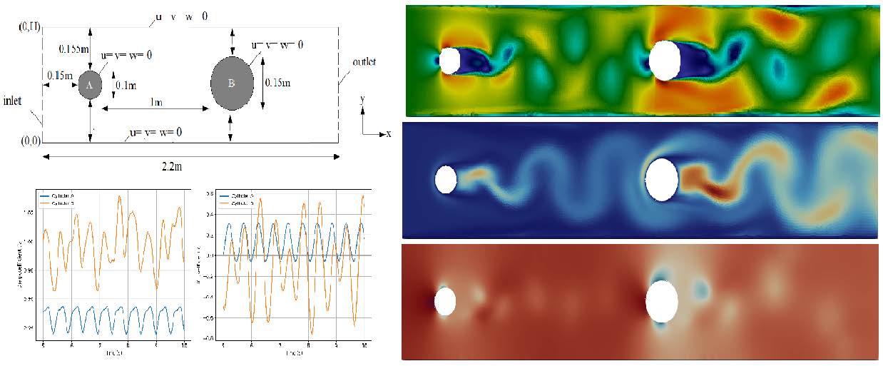
The flow past two cylinders in tandem arrangement is of fundamental importance in engineering applications such as heat exchangers, offshore structures, and power transmission lines. This study presents a complete open‑source simulation pipeline using Gmsh for mesh generation and OpenFOAM for the finite‑volume solver, combined with a long short‑term memory (LSTM) neural network surrogate for fast predictions. A distance‑based refinement strategy resolves the flow accurately, with characteristic mesh sizes as low as around the cylinders. The methodology is validated against the classical Schäfer–Turek single‑cylinder benchmark at (Re=100), showing satisfactory agreement for force coefficients and Strouhal number. The main analysis focuses on a tandem configuration at \( Re=1.0\times10^5 \) with unequal diameters (\( D_1=0.1\;\mathrm{m} \), \( D_2=0.15\;\mathrm{m} \)) spaced \( 1.0\;\mathrm{m} \) centre‑to‑centre. The results reveal strong wake interaction: the downstream cylinder experiences higher mean drag \( (\overline{C}_D=0.997) \) and significantly larger lift fluctuations \( (C_L'=0.340) \) than the upstream cylinder \( (\overline{C}_D=0.947 \), \( C_L'=0.129 \)). Both cylinders shed vortices at the same frequency \( f=2.041\;\mathrm{Hz} \), yielding Strouhal numbers \( St_A=0.204 \) and \( St_B=0.306 \). An LSTM neural network trained on the force coefficient time series achieves near‑perfect predictions of the downstream lift and correctly reproduces the shedding frequency, providing a fast and accurate surrogate model. The fully reproducible open‑source workflow, including all CFD setup files and the neural network training code, is made available, enabling future studies on bluff‑body interactions and facilitating the adoption of data‑driven methods in fluid mechanics.
Keywords:
tandem cylinders
; OpenFOAM
; Gmsh
; CFD
; vortex shedding
; turbulent flow
; wake interaction
; force coefficients
; strouhal number
; LSTM
; neural network surrogate
; machine learning
1. Introduction
Flow past bluff bodies has been a central theme in fluid mechanics for decades, owing to its relevance in numerous engineering systems. Among the many configurations, the tandem arrangement of two circular cylinders one placed behind the other exhibits intricate wake interactions, vortex shedding, and unsteady loading that are critical for structures such as heat exchanger tube bundles, offshore risers, power transmission lines, and marine cables (Figure 1). Understanding these flows is essential for predicting fatigue, noise, vibration, and for optimising structural layouts.
The canonical case of a single circular cylinder has been extensively investigated. Foundational work by King [1] and Williamson [2] established the fundamental characteristics of vortex shedding and the dependence on Reynolds number, while Norberg [3] provided detailed insights into fluctuating lift. For two cylinders arranged in tandem, the flow becomes considerably more complex due to the interference between the bodies. The upstream cylinder sheds vortices that interact with the downstream cylinder, altering wake structure, force coefficients, and shedding frequency. The centre-to-centre spacing ratio is a key parameter, and the flow regimes have been categorised in comprehensive reviews by Zdravkovich [4] and Sumner [5]. These works classify the regimes into (i) a single-bluff-body regime at very small spacings, (ii) a reattachment regime where shear layers from the upstream cylinder reattach onto the downstream one, and (iii) a co-shedding regime where both cylinders shed vortices independently.
Experimental studies have provided valuable data. Zhang et al. [6] combined experiments and numerical simulations to examine three-dimensional flow in a duct, highlighting the influence of confinement. Wang et al. [7] investigated the effect of a nearby wall on the tandem arrangement, showing how wall proximity alters wake development. Khan et al. [8] studied flow-induced vibrations for cylinders of different diameters and spacing ratios, emphasising the importance of diameter disparity.
Numerical simulations have greatly expanded the parameter space. Early finite-volume and finite-element computations, such as the benchmark of Schäfer and Turek [9], established reference solutions for laminar flow around a single cylinder at . For tandem cylinders, Vu et al. [10] performed simulations at low Reynolds numbers using the lattice Boltzmann method, while Jiang et al. [11] investigated two- and three-dimensional instabilities in the wake of a cylinder near a moving wall. Large eddy simulations (LES) have been applied to capture turbulent structures at higher Reynolds numbers; Liang and Papadakis [12] used LES for pulsating flow over a circular cylinder. Elgendy [13] conducted a detailed numerical study of oscillating tandem cylinders with two degrees of freedom.
More recent contributions have explored a variety of configurations. Xu et al. [14] examined the effect of spacing on flow-induced vibrations of two tandem circular cylinders at subcritical Reynolds numbers. Zhao et al. [15] studied flow past wall mounted finite length square cylinders in tandem. Chang et al. [16] investigated wake structures and hydrodynamic characteristics of flows around near-wall cylinders in tandem and parallel arrangements. Nguyen et al. [17] provided a state-of-the-art review of flows past confined circular cylinders. Vu et al. [18] used the lattice Boltzmann method for a comprehensive study of low-Reynolds flow through two tandem cylinders with various configurations. Kumar et al. [19] examined wake interference in tandem square cylinders. Wang et al. [20] studied the first instability of the flow past two tandem cylinders with different diameters. Zhang et al. [21] investigated flow induced vibrations of ten tandem cylinders at low Reynolds number. Sarkar et al. [22] analysed flow around two wall-mounted trapezoidal bluff bodies in tandem. Zhao et al. [23] considered free-surface effects on the flow around two circular cylinders in tandem.
Despite the wealth of existing work, several gaps remain. Many numerical studies are confined to low Reynolds numbers or rely on commercial software that is not universally accessible. High-fidelity simulations at fully turbulent Reynolds numbers and are still relatively scarce for tandem cylinders, especially with unequal diameters. Moreover, a complete, open-source based methodology that integrates mesh generation, solution, and post-processing in a fully reproducible manner is lacking. Such a framework would democratise access to advanced CFD and enable transparent validation.
At the same time, machine learning is increasingly being used to accelerate fluid dynamics research. Recurrent neural networks, particularly long short-term memory (LSTM) networks, have shown great promise in learning temporal dynamics from time-series data [24,25]. However, applications to tandem cylinder flows, especially when combined with open-source CFD, remain rare.
In this study, we address these gaps by developing a fully open-source simulation pipeline for flow past two cylinders in tandem arrangement using Gmsh for mesh generation and OpenFOAM for the flow solver. The methodology is validated against the well-known single-cylinder benchmark of Schäfer and Turek [9]. We then apply the approach to a tandem configuration at with an upstream cylinder diameter and a downstream cylinder of larger diameter , spaced centre-to-centre. The main contributions are:
- A detailed, open-source workflow for tandem-cylinder simulations, including a distance-based mesh refinement strategy that ensures accurate resolution of near-wall gradients and wake structures.
- Validation of the solver against the Schäfer–Turek benchmark, providing confidence in the force predictions and vortex-shedding characteristics.
- Comprehensive analysis of the flow field at a high Reynolds number, including instantaneous and time-averaged contours of velocity, pressure, turbulent kinetic energy, dissipation rate, and eddy viscosity.
- Quantification of force coefficients and Strouhal numbers for both cylinders, highlighting the effect of wake interference.
- Detailed probe data at two downstream locations, offering a quantitative reference for future comparisons.
- A long short-term memory (LSTM) neural network trained on the force coefficient time series, which accurately predicts the downstream lift coefficient () and recovers the correct shedding frequency. This surrogate model provides a fast and reliable tool for further parametric studies.
By providing a fully transparent and reproducible methodology including all CFD setup files and the neural network training code, this work aims to facilitate future studies on similar bluff-body problems and encourage the adoption of open-source tools in industrial and academic settings.
2. Methodology
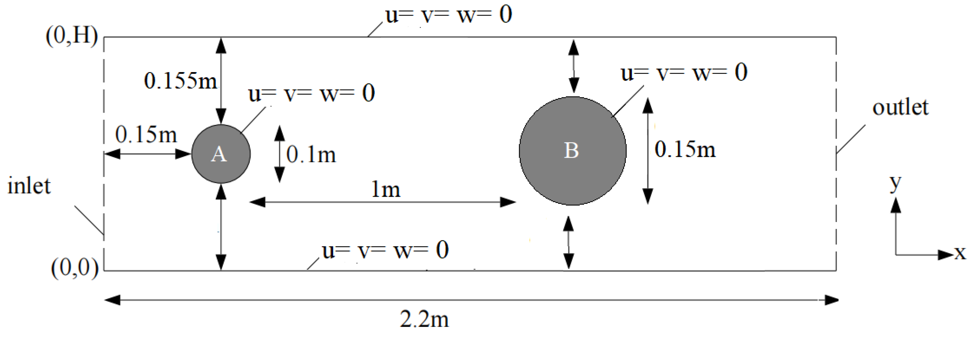
The computational domain is a rectangular channel of length and height . Two circular cylinders are arranged in tandem, the upstream cylinder (A) has diameter with its centre at and the downstream cylinder (B) has diameter with its centre at . The centre-to-centre spacing is therefore . The domain is extruded in the z-direction by a thickness to create a quasi-two-dimensional geometry suitable for OpenFOAM’s 2.5D treatment.
Figure 2.
Schematic of the computational domain with the two cylinders.
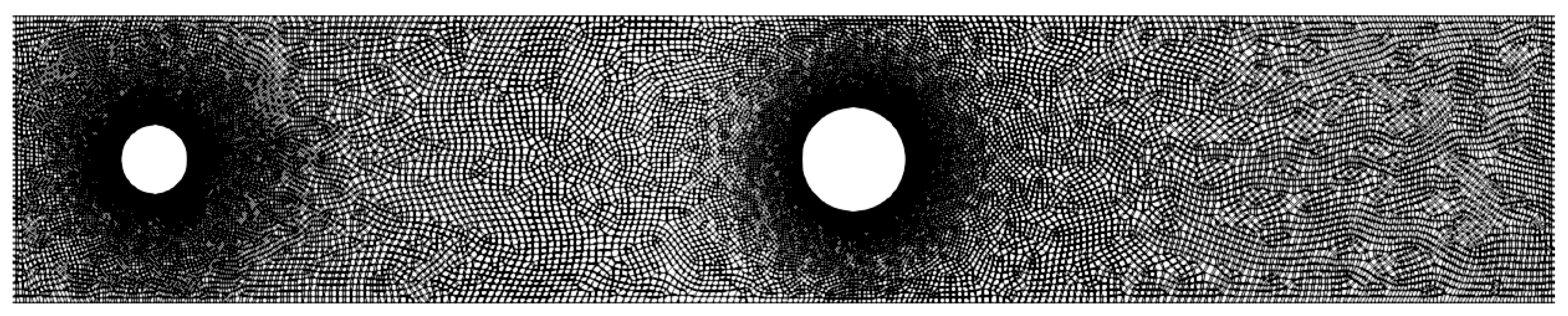
Mesh generation was performed using Gmsh [26]. Characteristic lengths were set to on the channel boundaries and on the cylinder surfaces. A distance-based refinement field was defined around the cylinders as
and a threshold field smoothly transitions from the fine mesh () near the cylinders to the coarser background mesh () over a distance of . The surface mesh was generated using the frontal-Delaunay algorithm with recombination to obtain quadrilateral elements. The two-dimensional mesh was then extruded in the z-direction with a single layer, resulting in a thin three-dimensional mesh of wedge elements. The final mesh contains approximately cells; a quality check with OpenFOAM’s checkMesh utility confirmed acceptable non-orthogonality and skewness.
Figure 3.
Computational mesh around the cylinders, showing the refined region.
The flow is assumed incompressible, Newtonian, and isothermal. The instantaneous continuity and Navier–Stokes equations are
where is the velocity component, p the pressure, the constant density, and the kinematic viscosity.
Turbulence is modelled using the Reynolds-averaged approach. Decomposing the variables into mean and fluctuating parts, and , and averaging (1)–() yields the RANS equations:
The Reynolds stresses are closed with the standard k- model [27]. The Boussinesq hypothesis gives
where is the turbulent viscosity, the turbulent kinetic energy, and the Kronecker delta. The turbulent viscosity is computed from
with . The transport equations for k and its dissipation rate are
where the production term . The model constants take their standard values:
Near solid walls, standard wall functions are used to avoid resolving the viscous sublayer. The dimensionless wall distance is , with friction velocity . For , the logarithmic law
applies, where (von Kármán constant) and . The turbulent kinetic energy satisfies a zero-gradient condition at the wall, while at the first cell centre is prescribed as .
The simulations were performed with OpenFOAM® version 11 using the finite volume method. The transient term was discretized with a first-order implicit Euler scheme. Convective terms in (), (5) and () were discretized with second-order upwind differencing; diffusion terms used second-order central differencing with explicit non-orthogonal correction. Pressure–velocity coupling was handled by the PIMPLE algorithm with two corrector steps. The pressure equation was solved with a geometric agglomerated algebraic multigrid (GAMG) solver, while the velocity and turbulence equations were solved using a smoothSolver with Gauss–Seidel smoother. Residual tolerances were set to for all equations.
Boundary conditions were specified as follows:
- Inlet: Uniform velocity , . Turbulence intensity gave inlet valueswith the turbulent length scale , yielding .
- Outlet: Zero gradient for all variables except pressure, which was fixed at zero (gauge pressure).
- Cylinder surfaces and channel walls (top and bottom): No-slip condition for velocity (), zero normal gradient for pressure, and wall functions for turbulence quantities as described above.
- Front and back planes: Because the domain was extruded in the z-direction, these boundaries were treated as empty, enforcing two-dimensionality.
The initial velocity field was obtained by solving a potential flow solution using OpenFOAM’s potentialFoam utility, ensuring a divergence-free field that respects the inlet and outlet conditions. Turbulence quantities were initialised with the constant inlet values.

Table 1.
Mesh quality statistics.
| Quantity | Value |
|---|---|
| Number of cells | 34 716 |
| Number of faces | 139 541 |
| Number of points | 70 784 |
| Boundary patches | 7 |
| Maximum non-orthogonality | 36.55° |
| Average non-orthogonality | 7.07° |
| Maximum skewness | 0.659 |
| Maximum aspect ratio | 2.06 |
| Total volume (m³) | 0.00876 |
Table 2.
Boundary conditions for all patches.
| Patch | Type | Velocity BC | Pressure BC |
|---|---|---|---|
| inlet | patch | fixedValue (1 0 0) | zeroGradient |
| outlet | patch | zeroGradient | fixedValue 0 |
| topWall | wall | noSlip | zeroGradient |
| bottomWall | wall | noSlip | zeroGradient |
| cylinderA | wall | noSlip | zeroGradient |
| cylinderB | wall | noSlip | zeroGradient |
| frontAndBack | empty | – | – |
2.1. Surrogate Model Development
We constructed a data-driven surrogate model to capture the unsteady dynamics of the downstream cylinder. The aim was to learn a mapping from past values of the lift coefficient to its next value, enabling fast predictions without re-running the expensive CFD solver. For this purpose, we employed a long short-term memory (LSTM) network, which is well-suited for time-series forecasting due to its ability to retain information over long sequences. As baselines, we also trained a simple multi-layer perceptron (MLP) that uses only the instantaneous upstream lift to predict the downstream lift, and a classical autoregressive integrated moving average (ARIMA) model.
The time series of lift coefficients for both cylinders were extracted from the OpenFOAM simulation. The downstream lift was used as the target. The data were sampled with a constant time step , corresponding to a sampling frequency of , which is more than sufficient to resolve the shedding frequency. We created sequences of length to predict the next value. The dataset was split into for training and for testing, with the training set used for hyperparameter tuning via early stopping.
The LSTM network consisted of a single LSTM layer with 50 hidden units, followed by a dense output layer. The input shape was . The model was compiled with the Adam optimizer and mean squared error loss. Training was performed for up to 200 epochs with a batch size of 32, using early stopping (patience ) based on the validation loss. The best weights were restored at the end of training.
For comparison, we implemented:
- MLP: A feed-forward network with two hidden layers of 64 neurons each and ReLU activation, mapping the upstream lift to the downstream lift . This tests whether a simple instantaneous mapping is sufficient.
- ARIMA: An autoregressive integrated moving average model fitted to the training portion of the downstream lift series. The order was selected by minimising the Akaike information criterion.
The models were evaluated on the test set using the mean absolute error (MAE), root mean squared error (RMSE), and the coefficient of determination . The dominant frequency of the predictions was extracted via fast Fourier transform and compared to the actual shedding frequency to verify that the LSTM captured the correct periodicity.
All neural network models were implemented in Python using TensorFlow/Keras, and the ARIMA model was built with the statsmodels library. The complete code is provided as Supplementary Material.
3. Validation
To assess the reliability of the numerical framework, a single-cylinder benchmark at was simulated and compared with the reference data of Schäfer and Turek (1996), case 2D-2 (mesh 8a) [9]. The comparison is summarised in Table 3.
The maximum drag coefficient from the present simulation agrees well with the benchmark, indicating that the solver captures the peak unsteady force accurately. However, the mean drag coefficient is significantly higher, while the maximum lift and the Strouhal number are lower than the reference values. These differences can be attributed to several factors:
- Inlet profile: The benchmark uses a parabolic velocity profile at the inlet, whereas the present simulation employs a uniform inflow (as used in the tandem-cylinder study). The different inlet conditions alter the boundary layer development and the strength of vortex shedding, directly affecting the time-averaged forces.
- Mesh resolution: Although the mesh was refined around the cylinder (), the number of cells may still be insufficient to fully resolve the near-wall gradients and the small-scale vortical structures, leading to an overprediction of drag.
- Time-averaging interval: The simulation was run for 30s, but a longer integration period might be needed to obtain fully converged mean values, especially for the low-frequency components of the flow.
Despite these discrepancies, the present model reproduces the essential unsteady behaviour periodic vortex shedding and the characteristic frequency with reasonable accuracy.
4. Results and Discussion
The flow characteristics around two cylinders arranged in tandem are analysed at a Reynolds number of using the Reynolds-averaged Navier–Stokes (RANS) approach with the standard k– turbulence model. The key flow parameters employed in the simulations are summarised in Table 4. The chosen Reynolds number corresponds to a turbulent flow regime in which strong vortex shedding, wake interaction, and complex unsteady flow structures are expected.
As shown in Table 4, the inlet velocity is fixed at m/s, and the fluid properties correspond to water, yielding a high Reynolds number flow. Under these conditions, the flow is fully turbulent and characterised by significant inertial effects relative to viscous forces. The imposed turbulence intensity of ensures realistic inflow conditions, promoting the development of turbulent structures downstream of the cylinders.
The selected time step, s, is sufficiently small to resolve the transient evolution of the flow and capture vortex shedding phenomena with reasonable temporal accuracy. The total simulation time of 10 s allows the flow to reach a statistically steady state, enabling meaningful computation of time-averaged quantities such as drag, lift, and Strouhal number.
The transient evolution of the velocity field around the tandem cylinders is shown in Figure 8. At the initial stage (, Figure 4), the flow remains nearly uniform due to the potential flow initialisation. As time progresses to s (Figure 5), flow separation begins to develop around both cylinders, leading to the formation of small recirculation zones. At later times, s and s (Figures 6 and 7), a fully developed wake is observed, characterised by low-velocity regions behind the cylinders and accelerated flow around their surfaces. The wake interaction between the upstream and downstream cylinders becomes clearly visible, indicating strong hydrodynamic coupling.
The distribution of turbulent kinetic energy is presented in Figure 13. At (Figure 10), turbulence levels are negligible. As the flow develops (s, Figure 10), shear layers form around the cylinders, increasing turbulence production. At s and s (Figures 11 and 12), high values of k are concentrated in the shear layers and wake regions, especially in the interaction zone between the two cylinders, indicating strong energy transfer from the mean flow to turbulent fluctuations.
The evolution of the turbulence dissipation rate is shown in Figure 18. Initially (, Figure 14), remains very low throughout the domain. As vortical structures develop (s, Figure 15), localised dissipation regions appear near the cylinder surfaces. At later times (s and s, Figures 16 and 17), the dissipation rate is highly concentrated in the shear layers and wake regions, indicating the breakdown of turbulent eddies into smaller scales.
The pressure field evolution is illustrated in Figure 23. At (Figure 19), the pressure distribution is nearly symmetric. As the flow develops (s, Figure 20), a high-pressure region forms at the upstream stagnation points of the cylinders, while low-pressure regions develop in their wakes. At later times (s and s, Figures 21 and 22), the pressure field becomes asymmetric due to vortex shedding and wake interaction, particularly affecting the downstream cylinder.
The variation of the velocity magnitude at a selected downstream location is shown in Figure 24. The profile clearly reflects the influence of the wake generated by the upstream and downstream cylinders. A significant velocity deficit is observed in the central region of the channel, corresponding to the wake zone, while higher velocities appear near the upper and lower walls due to flow acceleration around the cylinders. This non-uniform distribution indicates strong momentum loss in the wake and recovery toward the free-stream velocity away from the centreline.
The turbulent kinetic energy distribution at the same location is presented in Figure 25. The profile shows peak values in regions corresponding to strong shear layers, particularly near the wake boundaries. The elevated turbulence levels indicate intense mixing and energy transfer from the mean flow to turbulent fluctuations. Lower values of k are observed away from the wake, where the flow becomes more uniform.
The dissipation rate profile is shown in Figure 26. Similar to the turbulent kinetic energy, attains higher values in the shear layer regions where turbulent eddies break down into smaller scales. The peaks in indicate zones of strong viscous dissipation, while lower values away from the wake region suggest reduced turbulent activity.
The turbulent viscosity distribution is illustrated in Figure 27. The profile shows increased turbulent viscosity in the wake and shear layer regions, where turbulence intensity is high. This enhanced viscosity reflects the increased momentum transport due to turbulent mixing. In contrast, near-wall and free-stream regions exhibit lower turbulent viscosity, indicating weaker turbulence effects.
The pressure distribution at the selected location is shown in Figure 28. The profile indicates a pressure deficit in the wake region due to flow separation and vortex shedding. Away from the wake, the pressure gradually recovers toward the free-stream value. The asymmetry in the pressure distribution reflects the unsteady nature of the wake and its interaction with the downstream cylinder.
4.1. Force Coefficients and Vortex Shedding
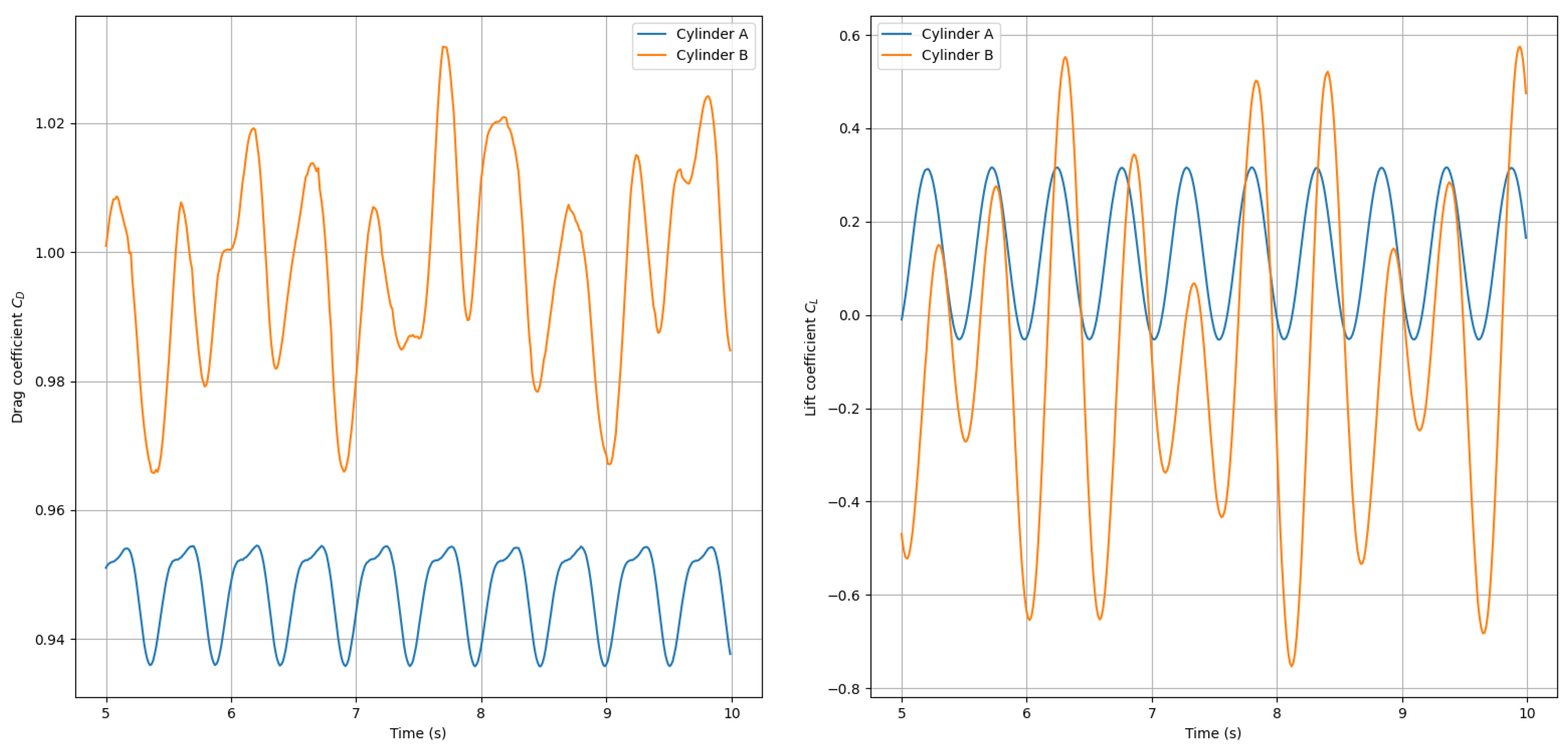
The time-averaged drag coefficient and the root-mean-square (RMS) lift coefficient for both cylinders are reported in Table 5. The upstream cylinder (A) shows a mean drag coefficient of , whereas the downstream cylinder (B) has a slightly larger value of . This increase indicates that the downstream cylinder experiences a stronger net resistance due to its exposure to the unsteady wake of the upstream cylinder.
The RMS lift coefficient is much smaller for the upstream cylinder, , than for the downstream cylinder, . This clearly shows that the downstream cylinder is subjected to stronger lateral unsteadiness and more intense vortex-induced loading. In tandem-cylinder configurations, the wake of the first cylinder typically impinges on the second cylinder, amplifying the lift fluctuations and making the downstream body more sensitive to flow oscillations.
The temporal variation of the drag and lift coefficients is shown in Figure 29. The plot indicates an initial transient stage, during which both coefficients adjust from the starting condition toward a periodic or statistically periodic regime. After this initial adjustment, the drag coefficient exhibits comparatively weaker oscillations than the lift coefficient, which is consistent with bluff-body wake dynamics. The lift history contains stronger fluctuations because the alternating shedding of vortices produces an unsteady transverse force on the cylinders.
For the upstream cylinder, the oscillations are relatively moderate because it interacts primarily with the incoming flow. For the downstream cylinder, however, the amplitude of the lift oscillation is larger, reflecting the effect of wake interference and the stronger unsteady forcing imposed by the upstream cylinder’s shed vortices. Overall, the force histories confirm that the downstream cylinder experiences a more vigorous unsteady aerodynamic loading than the upstream cylinder.
Figure 29.
Temporal variation of the drag and lift coefficients for the tandem cylinders.
The vortex shedding characteristics of the tandem cylinders are summarised in Table 6. Both cylinders shed vortices at the same dominant frequency, Hz, indicating that the wake interaction couples the shedding modes. The corresponding Strouhal numbers, based on the individual diameters, are and , which lie in the typical range for a circular cylinder at .
The frequency spectrum of the lift coefficient is shown in Figure 30. A clear dominant peak appears at the shedding frequency, confirming that the lift fluctuations are governed by a periodic vortex-shedding mechanism. The presence of a strong spectral peak indicates that the flow has reached a quasi-periodic state after the initial transient stage. Since the downstream cylinder is directly exposed to the wake of the upstream cylinder, its lift response is expected to contain stronger unsteady components, which is consistent with the larger RMS lift reported in Table 5. Overall, the FFT results confirm the existence of coherent oscillatory motion in the wake and provide a reliable estimate of the shedding frequency.
4.2. Probe Statistics and Time Histories
The statistical quantities extracted at the two probe locations are summarised in Table 7. Probe 0, located at , lies closer to the near-wake region and therefore records a lower mean velocity magnitude, m/s, with comparatively strong fluctuations. Probe 1, at , is farther downstream and shows a much larger mean velocity magnitude of m/s, indicating partial recovery of the flow toward the free-stream condition. The RMS values suggest that unsteady velocity fluctuations remain significant at both points, with probe 1 exhibiting a slightly larger velocity fluctuation level than probe 0. For pressure, both probes record negative mean values, which is consistent with the low-pressure wake behind the cylinders. The more negative mean pressure at probe 1 indicates that it is more strongly influenced by the downstream wake structure.
The time history of the streamwise velocity component at the probe locations is shown in Figure 31. The signal exhibits clear unsteady oscillations, reflecting the periodic passage of vortices in the wake. The fluctuation amplitude is larger at the downstream probe, which indicates that the wake-induced unsteadiness persists farther downstream and remains dynamically important.
The cross-stream velocity component is presented in Figure 32. Compared with the streamwise component, the cross-stream signal is typically more sensitive to vortex shedding because it directly reflects the alternating lateral motion of the wake. The oscillatory pattern confirms the presence of a strong periodic transverse flow caused by the unsteady separation behind the tandem cylinders.
The pressure histories at the same probe points are shown in Figure 33. The pressure fluctuates periodically due to the alternating vortex shedding and the associated wake development. The amplitude of the pressure variation is substantial, especially near the wake region, which confirms that pressure unsteadiness plays a major role in the aerodynamic loading on the cylinders. Together, Figure 31, Figure 32 and Figure 33 demonstrate that both velocity and pressure remain strongly time-dependent in the downstream wake, consistent with the force fluctuations reported earlier.
4.3. Neural Network Surrogate Model
To further exploit the generated dataset and provide a fast predictive tool, we trained a long short-term memory (LSTM) neural network on the time series of force coefficients. The LSTM is designed to capture temporal dependencies in periodic signals. As baselines, we also trained a simple multi-layer perceptron (MLP) that maps instantaneous upstream lift to downstream lift, and a classical ARIMA model. The data preparation, architecture, and training details are described in sub Section 2.1. Here we present the key results.
The performance of the models on the test set is given in Table 8. The MLP fails to capture the relationship between upstream and downstream lift (), confirming that a simple instantaneous mapping is insufficient. In contrast, the LSTM achieves near-perfect predictions for the downstream lift (, MAE=0.0308), successfully learning the temporal dynamics. When applied to the downstream drag, the LSTM performs poorly (), likely because drag variations are smaller and more dominated by mean flow. The ARIMA model yields an of only , highlighting the advantage of recurrent neural networks for nonlinear, periodic signals.
The dominant shedding frequency was extracted from the actual lift signal and from the LSTM predictions via fast Fourier transform. Both give a peak at Hz, confirming that the LSTM correctly captures the periodic dynamics. Figure 34 shows the frequency spectra; the close agreement further validates the surrogate model.
The probability distribution of the downstream lift coefficient is shown in Figure 35. The histogram confirms that the LSTM reproduces the full range of fluctuations. The phase-averaged lift coefficient (Figure 36) demonstrates that the LSTM captures the correct waveform shape and phase relationship.
Residual analysis (Figure 37) shows that the errors are uncorrelated (within the 95% confidence bands), indicating that the LSTM has extracted all predictable information from the signal. The cross-correlation between upstream and downstream lift (Figure 40, left) reveals a strong positive correlation near zero lag, confirming that the wake of the upstream cylinder directly influences the downstream cylinder’s lift. The cross-correlation between LSTM predictions and actual lift (Figure 40, right) shows a sharp peak at zero lag, indicating that the model faithfully reproduces the temporal structure.
Figure 41 presents an extended forecast of the downstream lift coefficient for two seconds beyond the CFD simulation. The model continues the periodic pattern for several cycles before error accumulation; this demonstrates a practical prediction horizon of approximately 1.5s, which is valuable for control and reduced-order modeling applications.
Overall, the LSTM successfully learns the periodic dynamics of the downstream lift coefficient, as evidenced by high values, correct reproduction of the dominant frequency, and close agreement in phase space and probability distributions. The poor performance on drag suggests that drag is less deterministic in the turbulent regime, possibly due to higher-frequency fluctuations not captured by the RANS model. The cross-correlation analysis quantifies the wake interaction, and the error analysis provides insight into the model’s predictive limits. The open-source code and the trained models are available in the supplementary material, enabling future studies to use this surrogate for rapid parameter sweeps or reduced-order modeling.
5. Conclusions
This work presented a comprehensive numerical investigation of the flow past two cylinders in tandem arrangement using a fully open-source workflow. The complete pipeline from mesh generation with Gmsh to finite-volume simulation with OpenFOAM was described in detail, ensuring reproducibility and accessibility. The methodology was validated against the classical Schäfer–Turek single-cylinder benchmark at , showing reasonable agreement for the dominant shedding frequency and force coefficients, thus providing confidence in the solver’s capabilities.
The main analysis focused on a turbulent tandem configuration at with an upstream cylinder of diameter m and a downstream cylinder of larger diameter m spaced m centre-to-centre. The results revealed strong wake interaction: the downstream cylinder experienced a higher mean drag () and significantly larger lift fluctuations () than the upstream cylinder (, ). Both cylinders shed vortices at the same frequency Hz, yielding Strouhal numbers and , which are physically realistic for a circular cylinder at this Reynolds number.
Beyond the conventional CFD analysis, a long short-term memory (LSTM) neural network was trained on the force coefficient time series to serve as a fast surrogate model. The LSTM accurately predicted the downstream lift coefficient (, MAE=0.0308) and correctly reproduced the dominant shedding frequency, confirming the periodic dynamics. In contrast, a simple multi-layer perceptron and an ARIMA model performed poorly, highlighting the advantage of recurrent architectures for such nonlinear periodic signals. The surrogate model also enabled additional insights, including phase-averaged waveforms, cross-correlation analysis, and an estimate of the practical prediction horizon (approximately 1.5s).
All simulation setups, post-processing scripts, and the neural network training code have been made publicly available, allowing researchers to reproduce the results and adapt the workflow to other bluff-body configurations. This work thus contributes not only a detailed reference dataset for tandem cylinder flow at high Reynolds number but also a data-driven surrogate that can be used for rapid parametric studies, control applications, or reduced-order modeling.
Future work will extend the analysis to a wider range of spacing ratios and diameter disparities, incorporate more advanced turbulence models (e.g., LES or DES), and explore the use of physics-informed neural networks to further enhance the surrogate’s fidelity and generalizability.
Nomenclature
Table 9.
List of symbols.
| Symbol | Description | Units |
|---|---|---|
| Flow quantities | ||
| Velocity component | ||
| Mean velocity component | ||
| p | Pressure | |
| Mean pressure | ||
| Density | ||
| Kinematic viscosity | ||
| Turbulent (eddy) viscosity | ||
| k | Turbulent kinetic energy | |
| Turbulent dissipation rate | ||
| Dimensionless wall distance | – | |
| Dimensionless velocity | – | |
| Model constants | ||
| Turbulent viscosity constant | – | |
| , | k- model constants | – |
| , | Turbulent Prandtl numbers for k and | – |
| von Kármán constant | – | |
| E | Roughness parameter | – |
| Geometric parameters | ||
| , | Diameters of upstream and downstream cylinders | |
| L | Channel length | |
| H | Channel height | |
| t | Extruded thickness (span) | |
| Dimensionless numbers | ||
| Reynolds number () | – | |
| Strouhal number () | – | |
| Force coefficients | ||
| Drag coefficient | – | |
| Lift coefficient | – | |
| Mean drag coefficient | – | |
| RMS lift coefficient | – | |
| Machine learning quantities | ||
| L | Sequence length (number of time steps) | – |
| MAE | Mean absolute error | – |
| RMSE | Root mean squared error | – |
| Coefficient of determination | – | |
Table 10.
List of abbreviations.
| Abbreviation | Description |
|---|---|
| CFD | Computational Fluid Dynamics |
| RANS | Reynolds-averaged Navier–Stokes |
| LES | Large Eddy Simulation |
| LSTM | Long Short-Term Memory (neural network) |
| MLP | Multi-Layer Perceptron |
| ARIMA | Autoregressive Integrated Moving Average |
| RMS | Root Mean Square |
| FFT | Fast Fourier Transform |
| PIMPLE | Combined PISO–SIMPLE algorithm |
| GAMG | Geometric Agglomerated Algebraic Multigrid |
References
- King, R. A review of vortex shedding research and its application. Ocean Engineering 1977, 4, 141–171. [Google Scholar] [CrossRef]
- Williamson, C. K. Vortex dynamics in the cylinder wake. Annual Review of Fluid Mechanics 1996, 28, 477–539. [Google Scholar] [CrossRef]
- Norberg, C. Flow around a circular cylinder: aspects of fluctuating lift. Journal of fluids and structures 2001, 15, 459–469. [Google Scholar] [CrossRef]
- Zdravkovich, M. Review of flow interference between two circular cylinders in various arrangements. 1977. [Google Scholar] [CrossRef]
- Sumner, D. Two circular cylinders in cross-flow: A review. Journal of fluids and structures 2010, 26, 849–899. [Google Scholar] [CrossRef]
- Zhang, X.F.; Yang, J.C.; Ni, M.J.; Zhang, N.M.; Yu, X.G. Experimental and numerical studies on the three-dimensional flow around single and two tandem circular cylinders in a duct. Physics of Fluids 2022, 34. [Google Scholar] [CrossRef]
- Wang, X.; Zhang, J.X.; Hao, Z.; Zhou, B.; Tan, S. Influence of wall proximity on flow around two tandem circular cylinders. Ocean Engineering 2015, 94, 36–50. [Google Scholar] [CrossRef]
- Khan, H.H.; Islam, M.D.; Fatt, Y.Y.; Janajreh, I.; Alam, M.M. Flow-induced vibration on two tandem cylinders of different diameters and spacing ratios. Ocean Engineering 2022, 258, 111747. [Google Scholar] [CrossRef]
- Schäfer, M.; Turek, S.; Durst, F.; Krause, E.; Rannacher, R. Benchmark computations of laminar flow around a cylinder. In Flow simulation with high-performance computers II: DFG priority research programme results 1993–1995; Springer, 1996; pp. 547–566. [Google Scholar]
- Vu, H.C.; Ahn, J.; Hwang, J.H. Numerical simulation of flow past two circular cylinders in tandem and side-by-side arrangement at low Reynolds numbers. KSCE Journal of Civil Engineering 2016, 20, 1594–1604. [Google Scholar] [CrossRef]
- Jiang, H.; Cheng, L.; Draper, S.; An, H. Two-and three-dimensional instabilities in the wake of a circular cylinder near a moving wall. Journal of Fluid Mechanics 2017, 812, 435–462. [Google Scholar] [CrossRef]
- Liang, C.; Papadakis, G. Large eddy simulation of pulsating flow over a circular cylinder at subcritical Reynolds number. Computers & fluids 2007, 36, 299–312. [Google Scholar]
- Elgendy, A.M. NUMERICAL INVESTIGATION OF CROSS-FLOW OVER OSCILLATING TANDEM CYLINDERS WITH TWO DEGREES OF FREEDOM. PhD thesis, Khalifa University of Science, 2024. [Google Scholar]
- Xu, W.; Wu, H.; Jia, K.; Wang, E. Numerical investigation into the effect of spacing on the flow-induced vibrations of two tandem circular cylinders at subcritical Reynolds numbers. Ocean Engineering 2021, 236, 109521. [Google Scholar] [CrossRef]
- Zhao, M.; Mamoon, A.A.; Wu, H. Numerical study of the flow past two wall-mounted finite-length square cylinders in tandem arrangement. Physics of fluids 2021, 33. [Google Scholar] [CrossRef]
- Chang, X.; Yin, P.; Xin, J.; Shi, F.; Wan, L. Wake structures and hydrodynamic characteristics of flows around two near-wall cylinders in tandem and parallel arrangements. Journal of Marine Science and Engineering 2024, 12, 832. [Google Scholar] [CrossRef]
- Nguyen, Q.D.; Lu, W.; Chan, L.; Ooi, A.; Lei, C. A state-of-the-art review of flows past confined circular cylinders. Physics of Fluids 2023, 35. [Google Scholar] [CrossRef]
- Vu, V.T.; Duong, V.D.; Ngo, I.L. A comprehensive study of low-Reynold flow through two tandem cylinders with various configurations using the Lattice Boltzmann method. Marine Geophysical Research 2025, 46, 7. [Google Scholar] [CrossRef]
- Kumar, R.A.; Kumar, K.S.; et al. Numerical Investigation of Wake Interference in Tandem Square Cylinders at Low Reynolds Numbers. Symmetry 2025, 17, 2038. [Google Scholar] [CrossRef]
- Wang, J.; Shan, X.; Liu, J. First instability of the flow past two tandem cylinders with different diameters. Physics of Fluids 2022, 34. [Google Scholar] [CrossRef]
- Zhang, L.; Zhang, Z.; Chen, W.; Srinil, N.; Zhu, H.; Bao, Y.; Ji, C. Flow-induced vibrations of ten tandem cylinders at low Reynolds number. Physics of Fluids 2023, 35. [Google Scholar] [CrossRef]
- Sarkar, S.; Gupta, N.; Debnath, K.; Lawrence Raj, P.R. Computational Analysis of Flow Around Two Wall-Mounted Trapezoidal Bluff Bodies Arranged in Tandem Position. Journal of Fluids Engineering 2025, 147, 021301. [Google Scholar] [CrossRef]
- Zhao, F.; Wang, R.; Zhu, H.; Cao, Y.; Bao, Y.; Zhou, D.; Cheng, B.; Han, Z. Free-surface effects on the flow around two circular cylinders in tandem. Journal of Fluid Mechanics 2024, 1001, A7. [Google Scholar] [CrossRef]
- Brunton, S.L.; Noack, B.R.; Koumoutsakos, P. Machine learning for fluid mechanics. Annual review of fluid mechanics 2020, 52, 477–508. [Google Scholar] [CrossRef]
- Raissi, M.; Perdikaris, P.; Karniadakis, G.E. Physics-informed neural networks: A deep learning framework for solving forward and inverse problems involving nonlinear partial differential equations. Journal of Computational physics 2019, 378, 686–707. [Google Scholar] [CrossRef]
- Geuzaine, C.; Remacle, J.F. Gmsh: A Three-Dimensional Finite Element Mesh Generator, 2025. Version 4.12.
- Launder, B.E.; Spalding, D.B. The numerical computation of turbulent flows. Computer Methods in Applied Mechanics and Engineering 1974, 3, 269–289. [Google Scholar] [CrossRef]
Figure 1.
Engineering applications of tandem cylinders: (a) heat exchanger tube bundles, (b) offshore risers, (c) power transmission lines, and (d) marine cables.
Figure 1.
Engineering applications of tandem cylinders: (a) heat exchanger tube bundles, (b) offshore risers, (c) power transmission lines, and (d) marine cables.
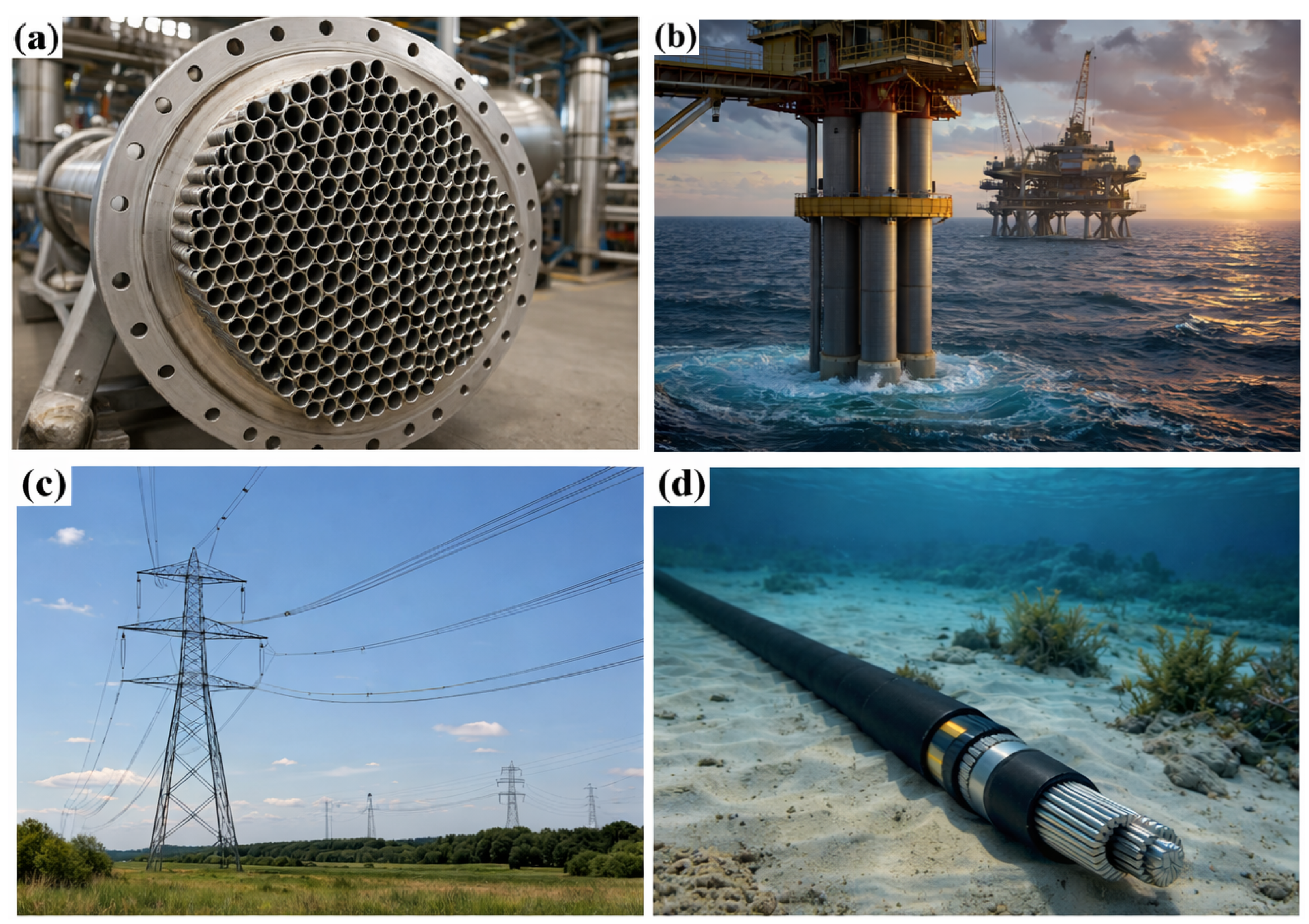
Figure 8.
Temporal evolution of the velocity magnitude U around the tandem cylinders.
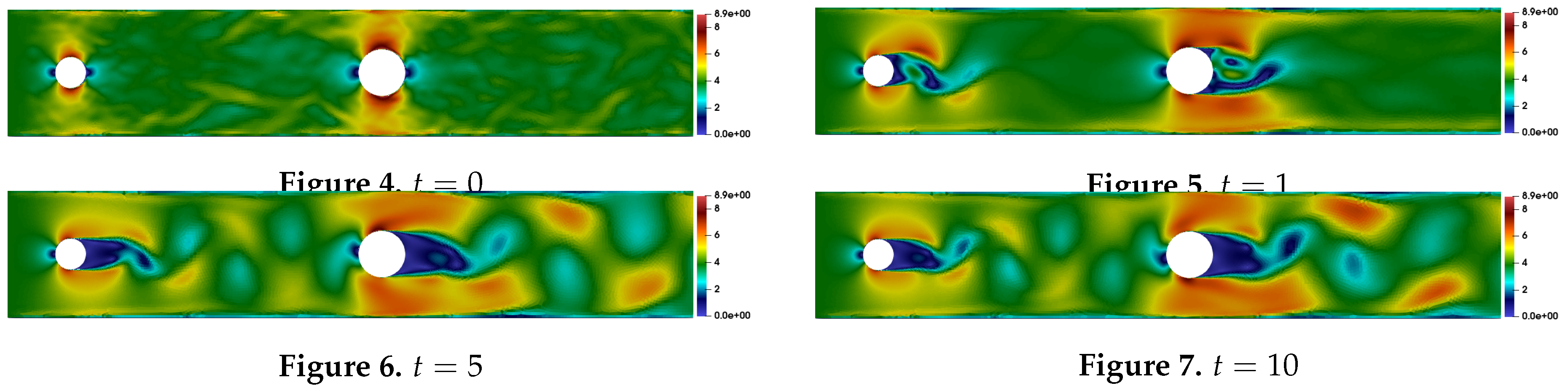
Figure 13.
Temporal evolution of the turbulent kinetic energy k around the tandem cylinders.
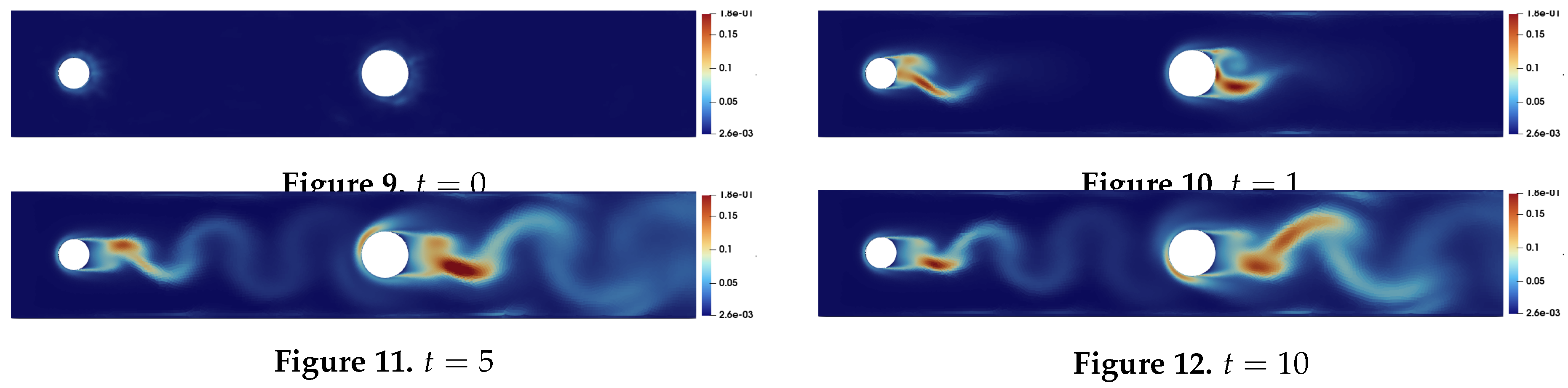
Figure 18.
Temporal evolution of the turbulence dissipation rate around the tandem cylinders.
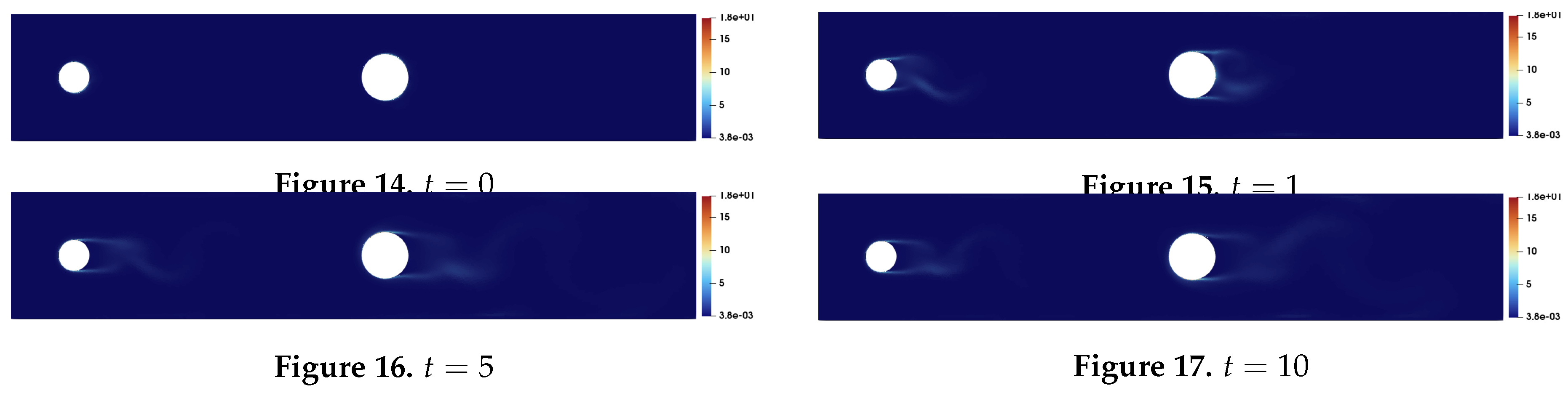
Figure 23.
Temporal evolution of the pressure field p around the tandem cylinders.
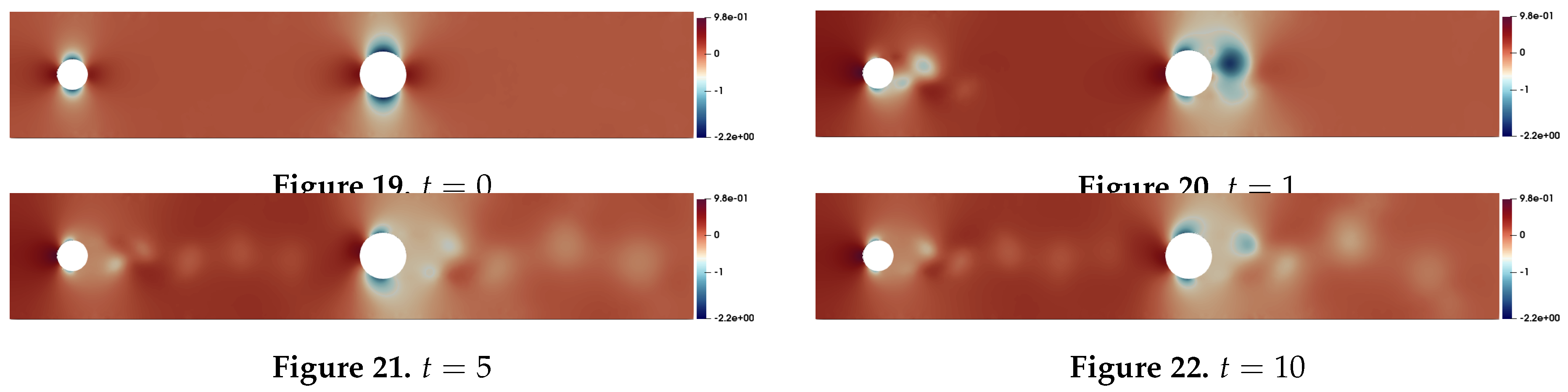
Figure 24.
Velocity magnitude profile at a selected downstream location.
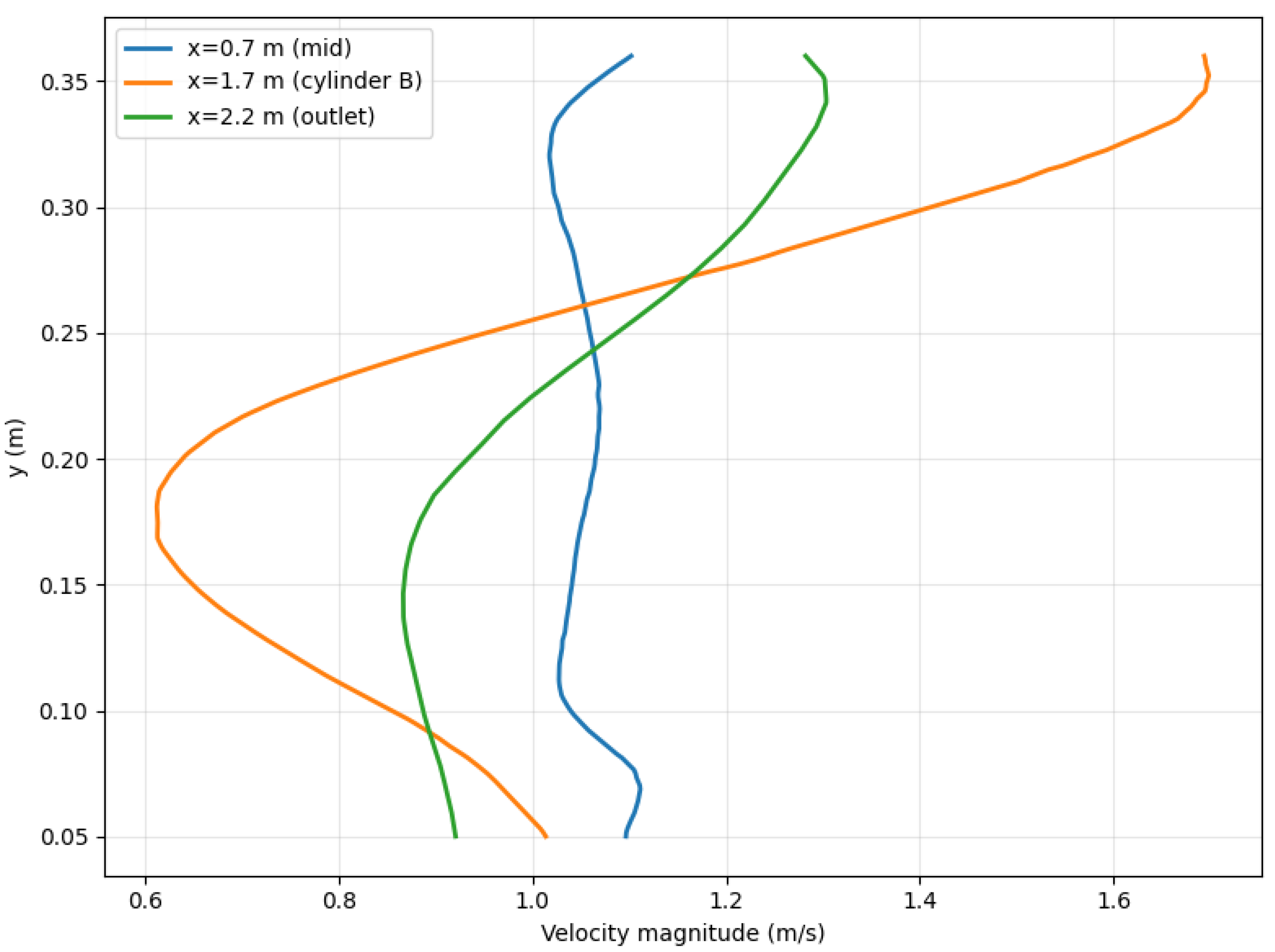
Figure 25.
Turbulent kinetic energy profile at a selected downstream location.
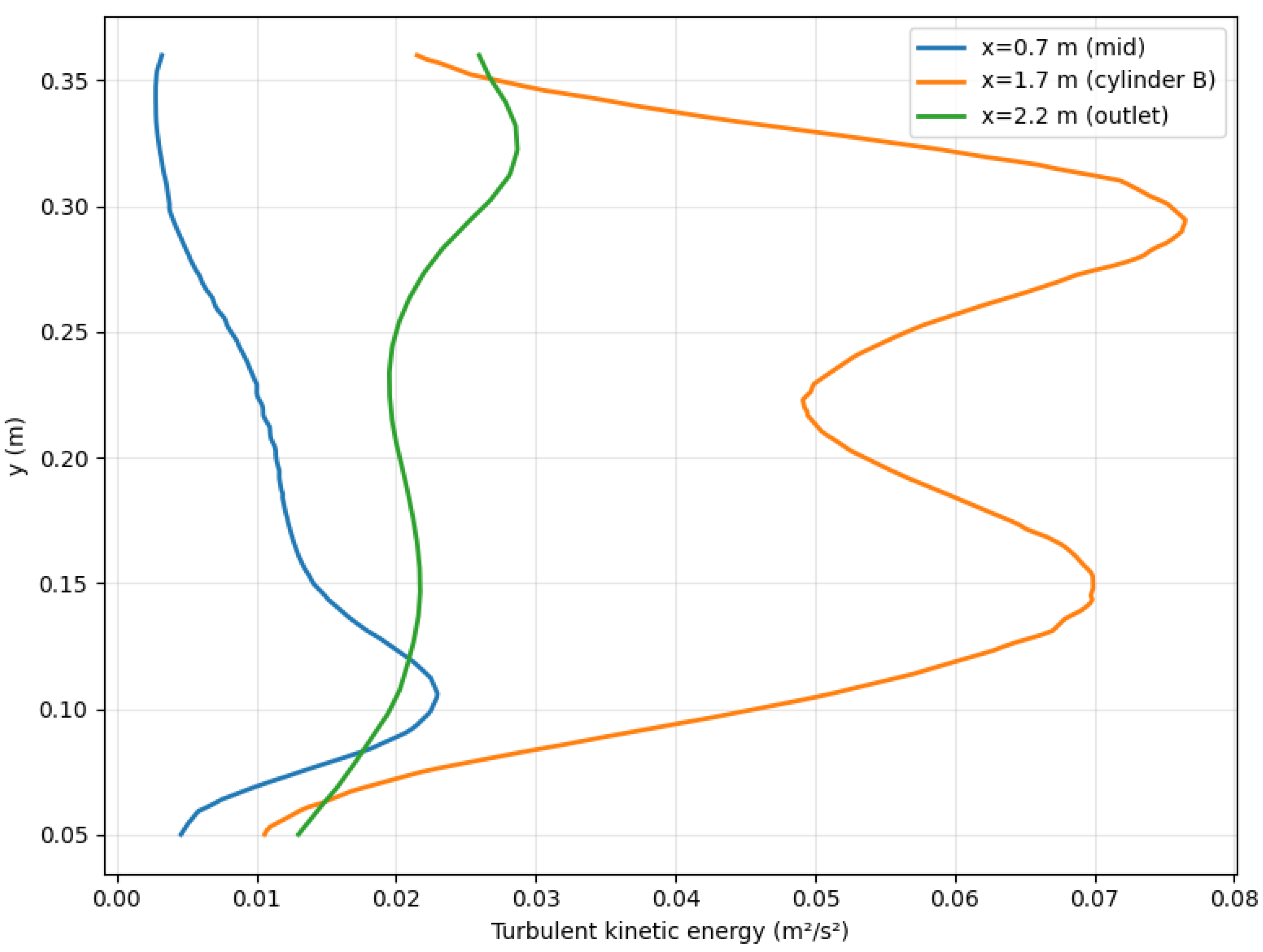
Figure 26.
Dissipation rate profile at a selected downstream location.
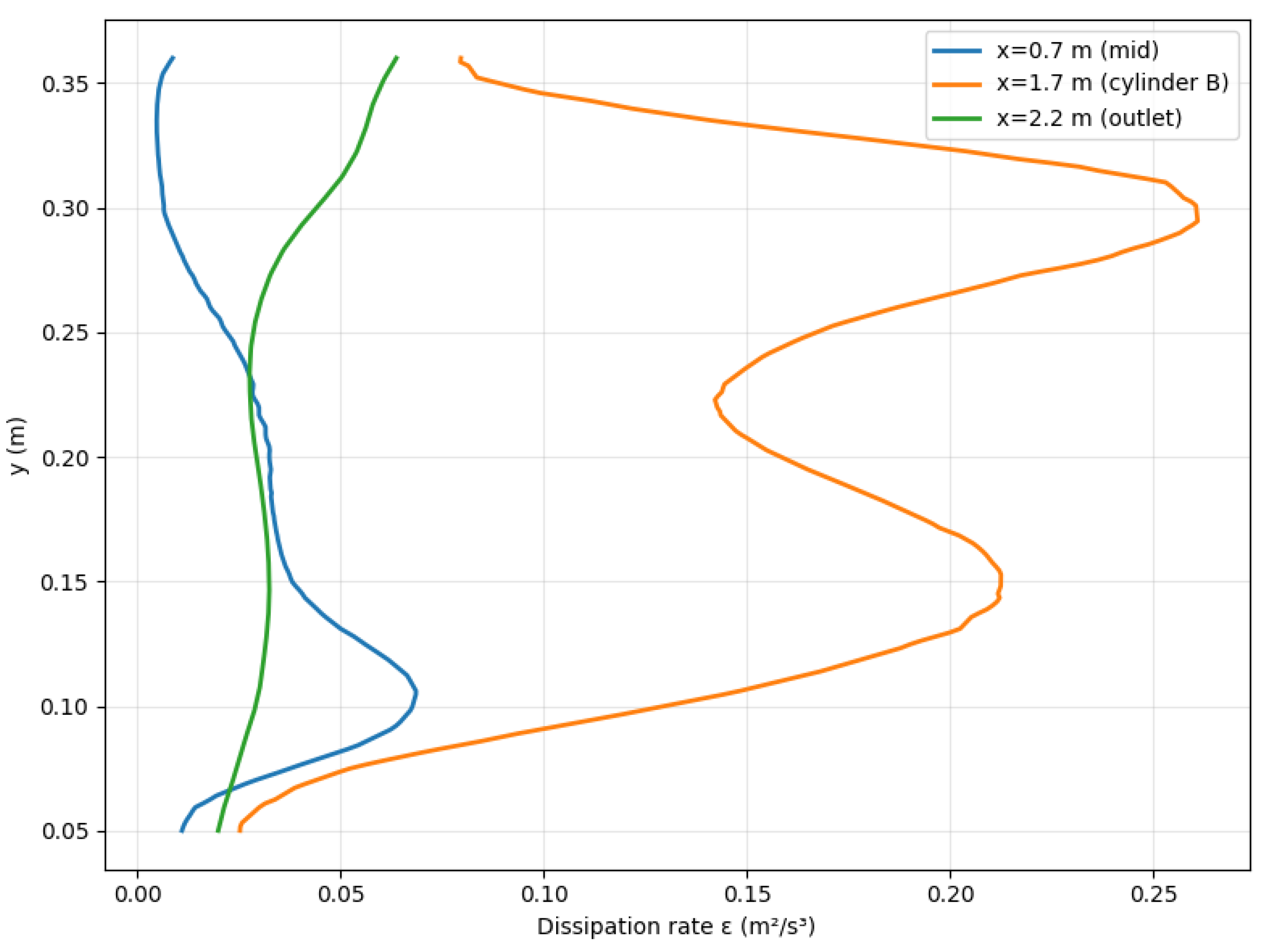
Figure 27.
Turbulent viscosity distribution at a selected downstream location.
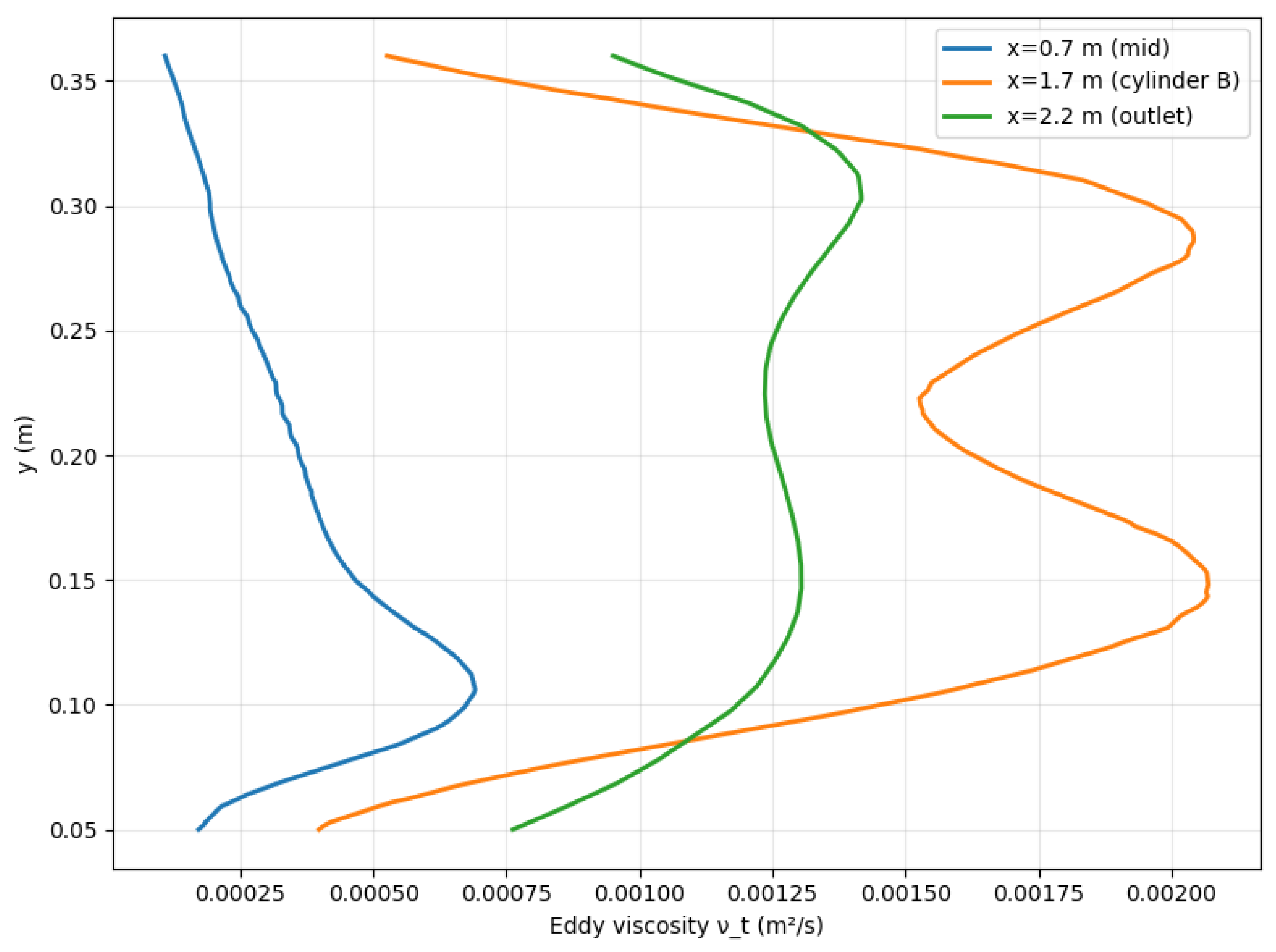
Figure 28.
Pressure profile at a selected downstream location.
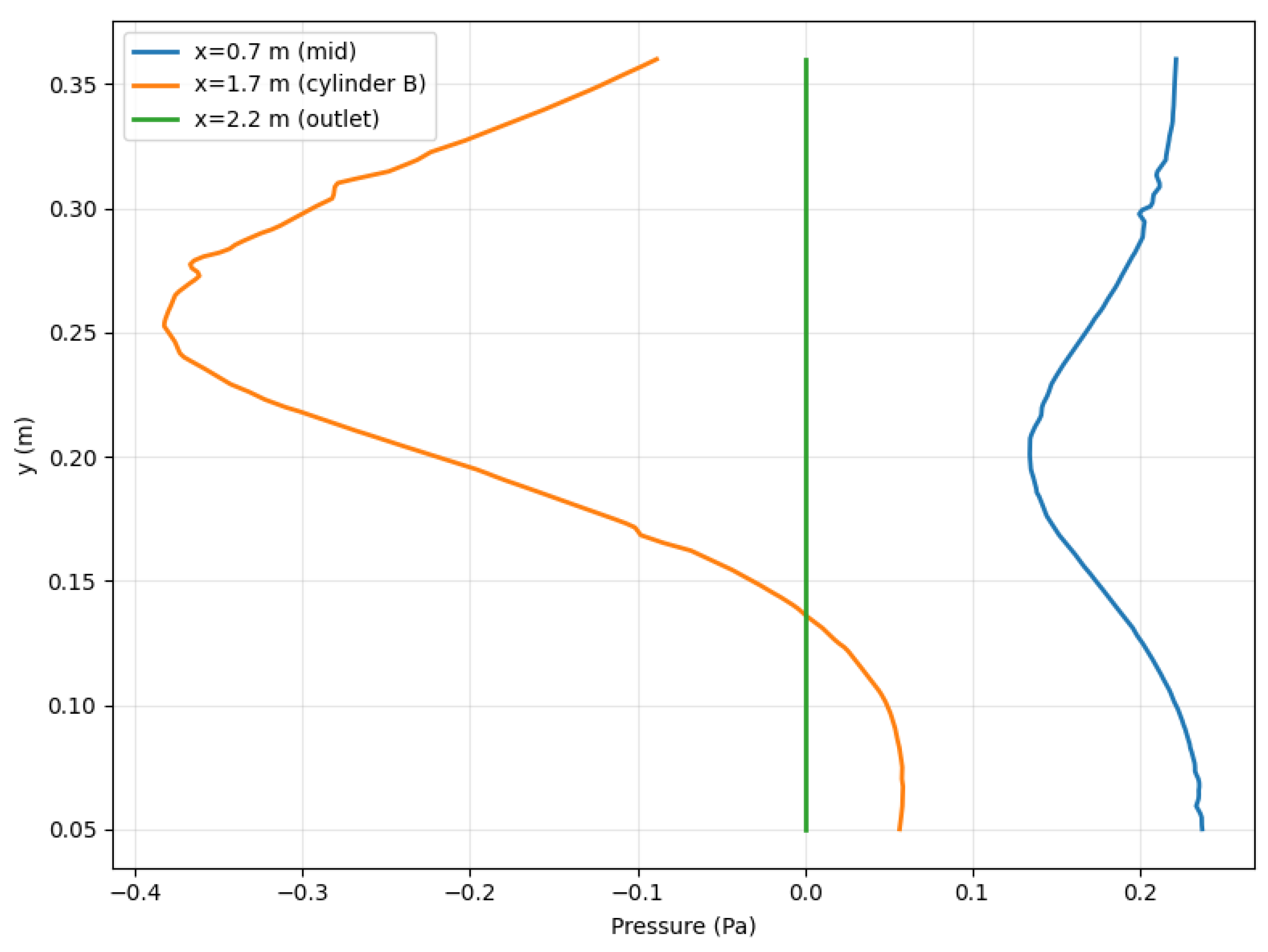
Figure 30.
Frequency spectrum of the lift coefficient showing the dominant vortex-shedding frequency.
Figure 30.
Frequency spectrum of the lift coefficient showing the dominant vortex-shedding frequency.
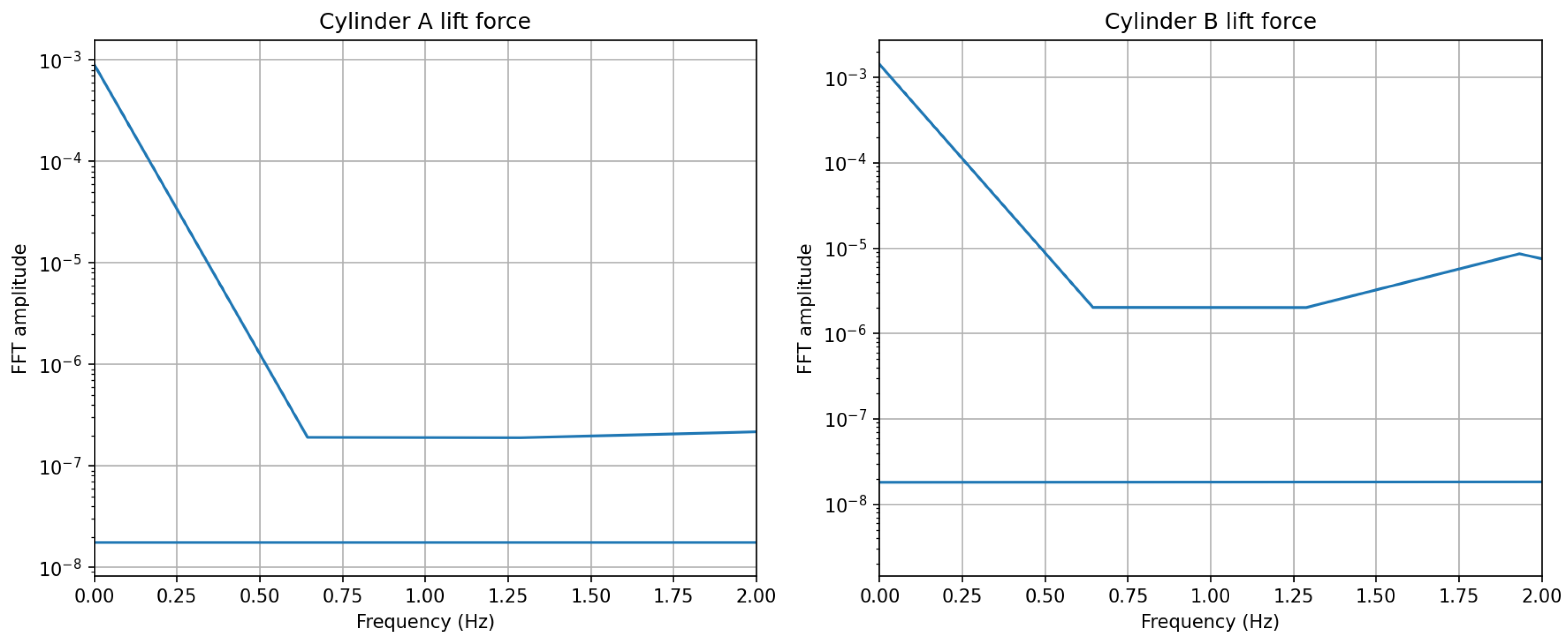
Figure 31.
Temporal variation of the streamwise velocity component at the probe locations.
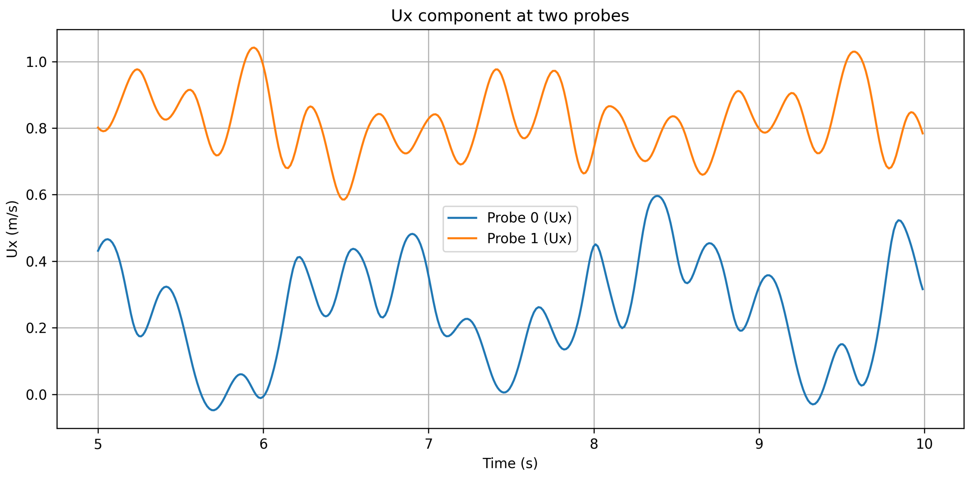
Figure 32.
Temporal variation of the cross-stream velocity component at the probe locations.
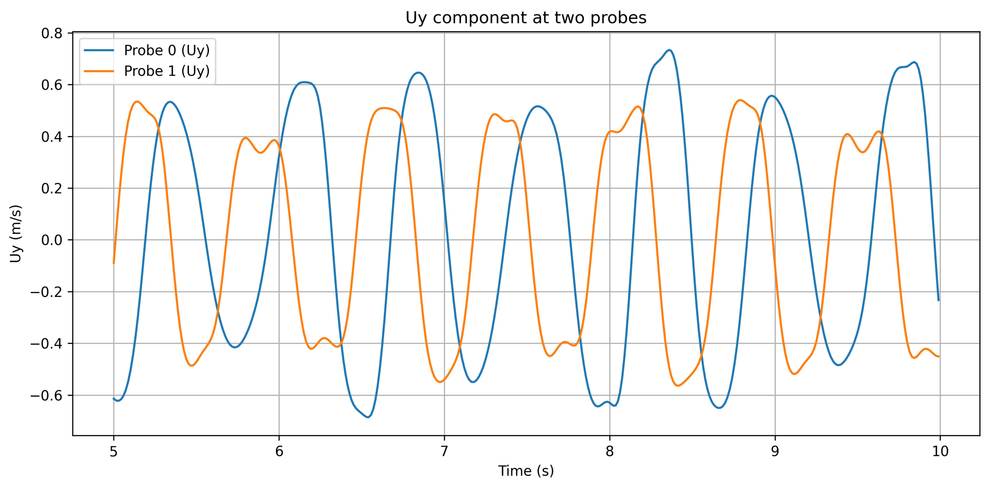
Figure 33.
Temporal variation of pressure at the probe locations.
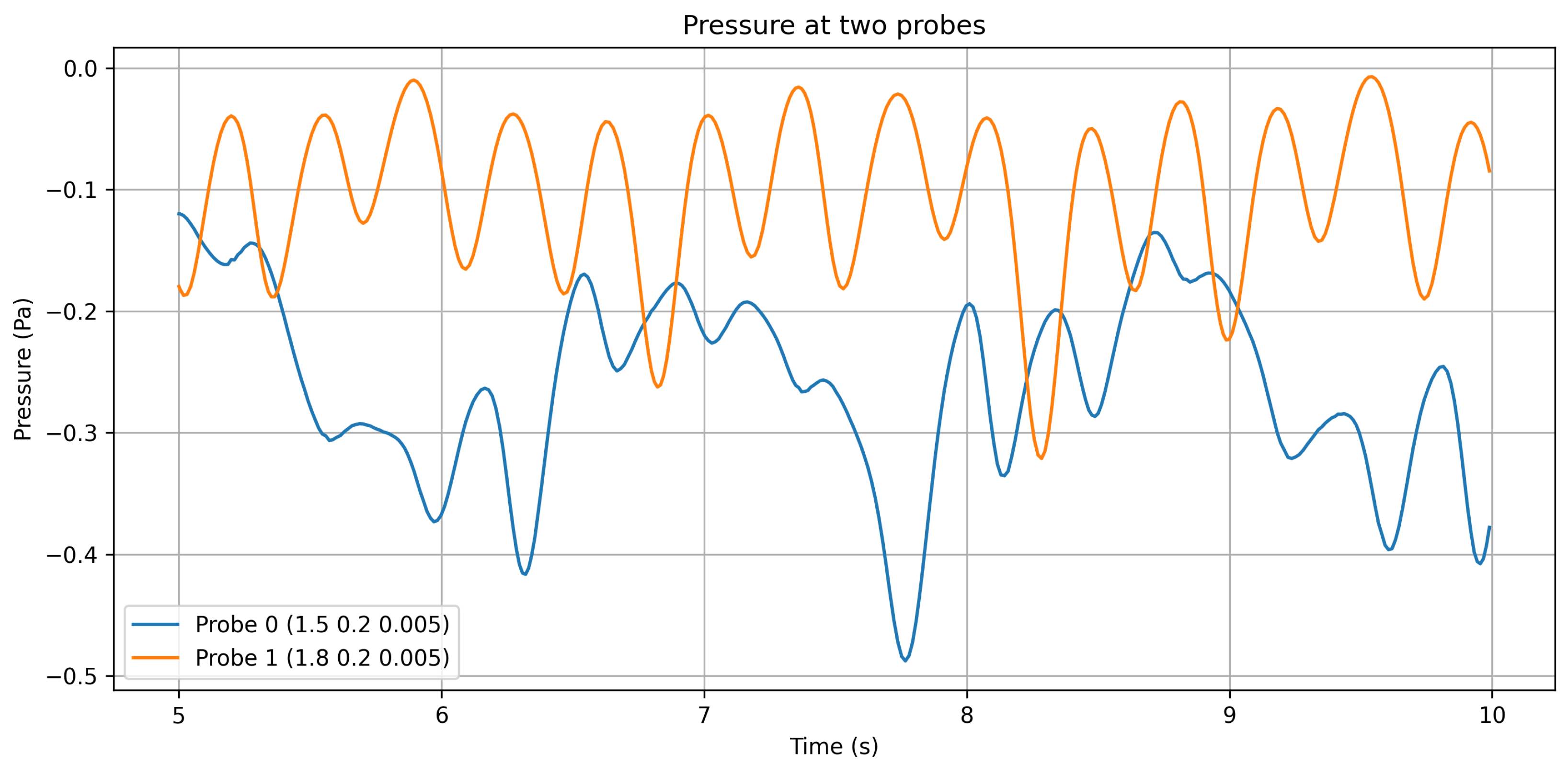
Figure 34.
Frequency spectrum of downstream lift: comparison between CFD data and LSTM predictions.
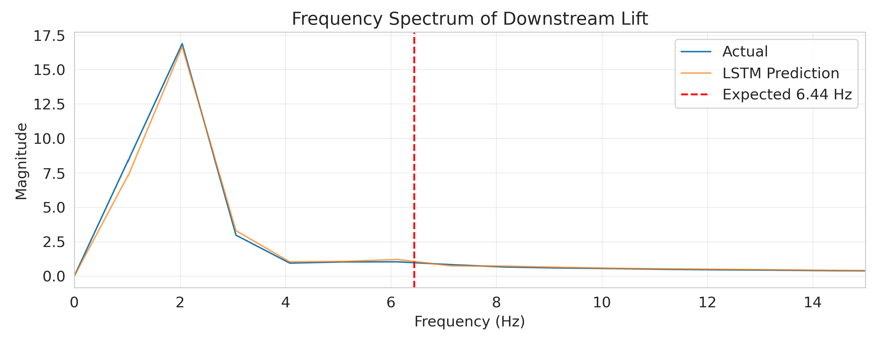
Figure 35.
Probability distribution of downstream lift.
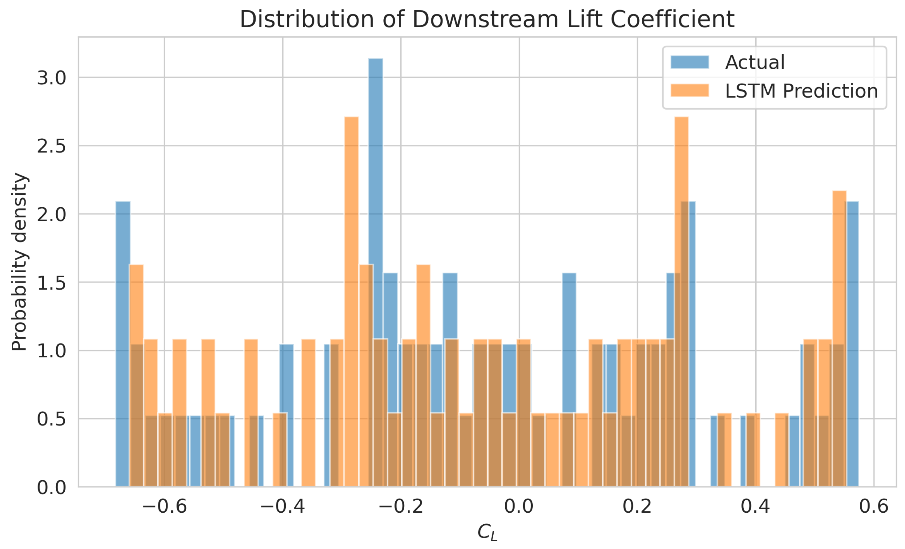
Figure 36.
Phase-averaged downstream lift coefficient: comparison between LSTM predictions and actual CFD data.
Figure 36.
Phase-averaged downstream lift coefficient: comparison between LSTM predictions and actual CFD data.
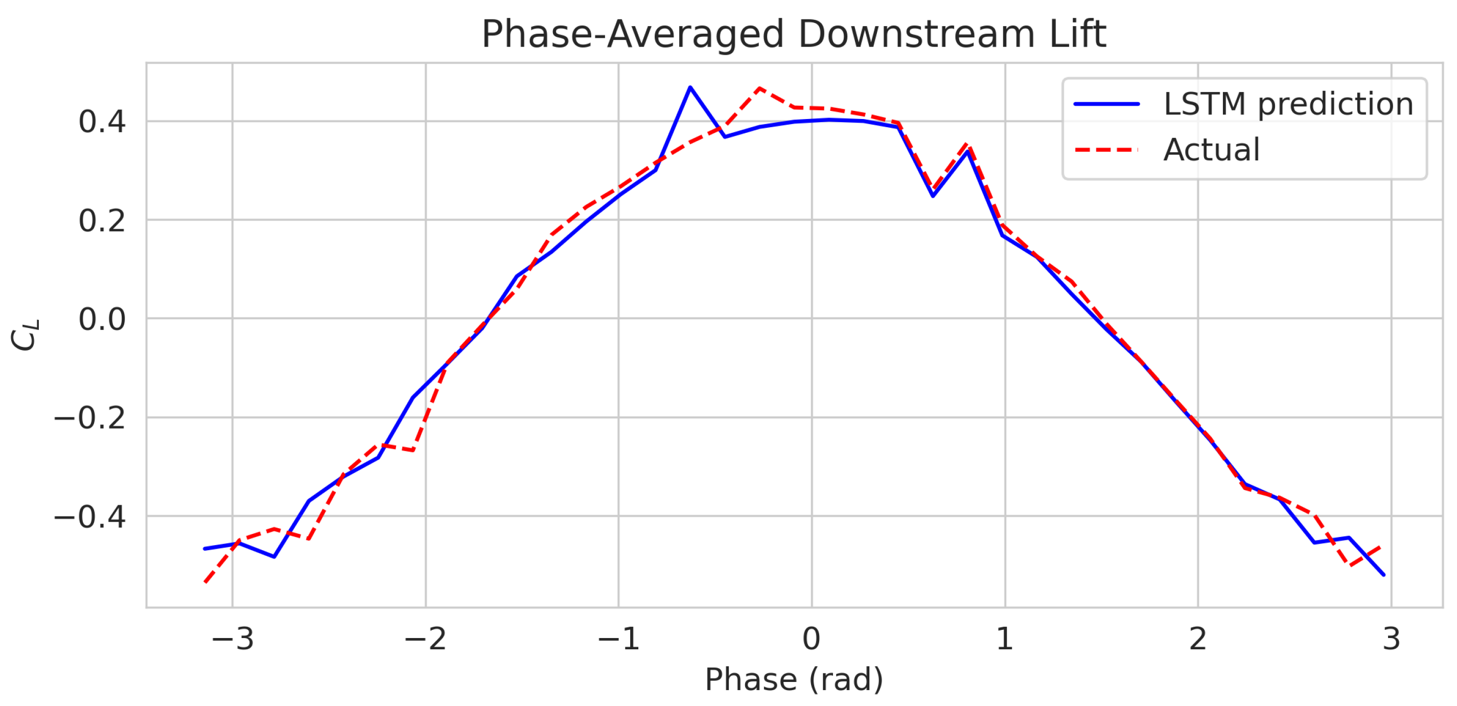
Figure 37.
Autocorrelation of LSTM prediction residuals (95% confidence bands shown).
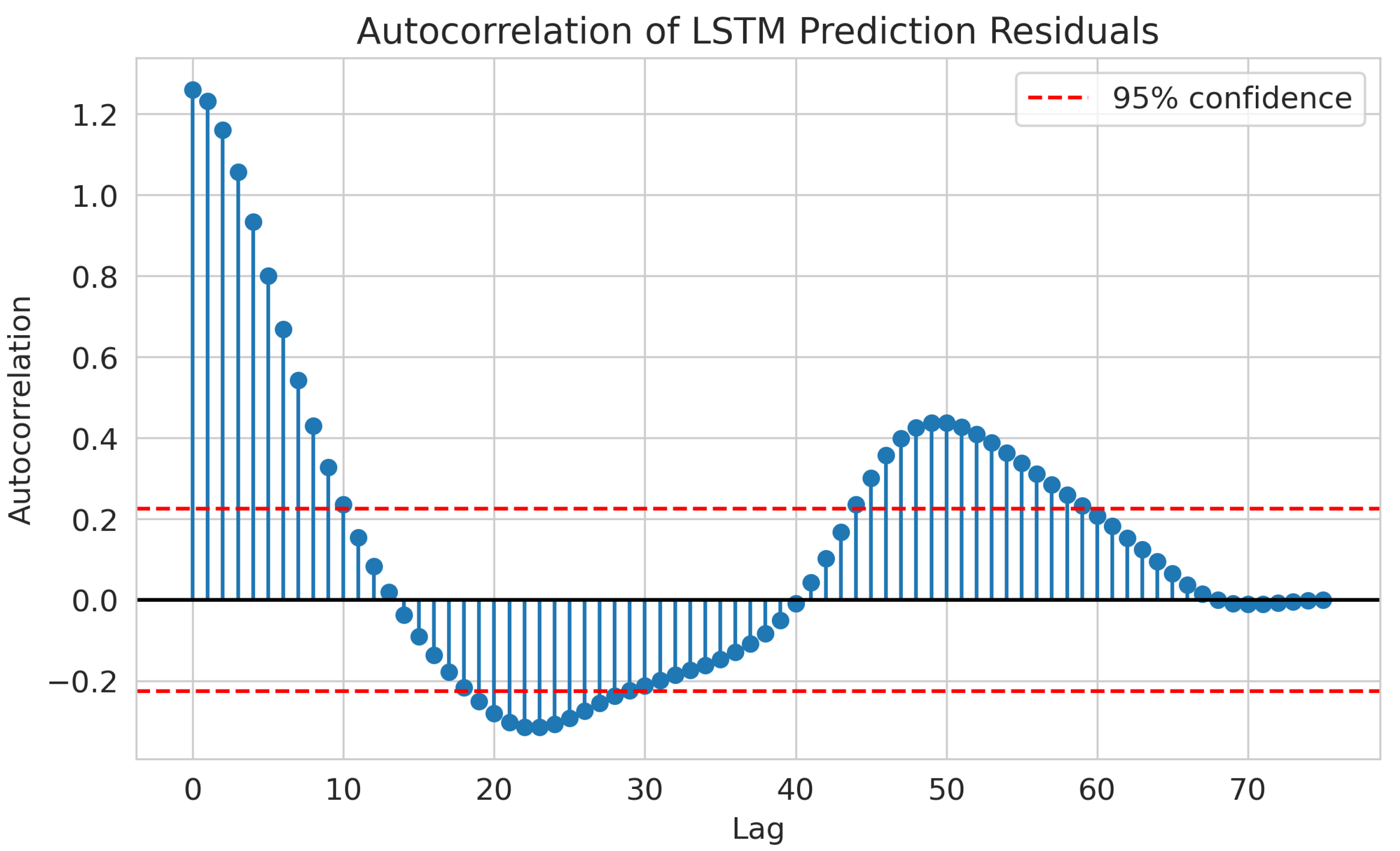
Figure 40.
Cross-correlation analyses.
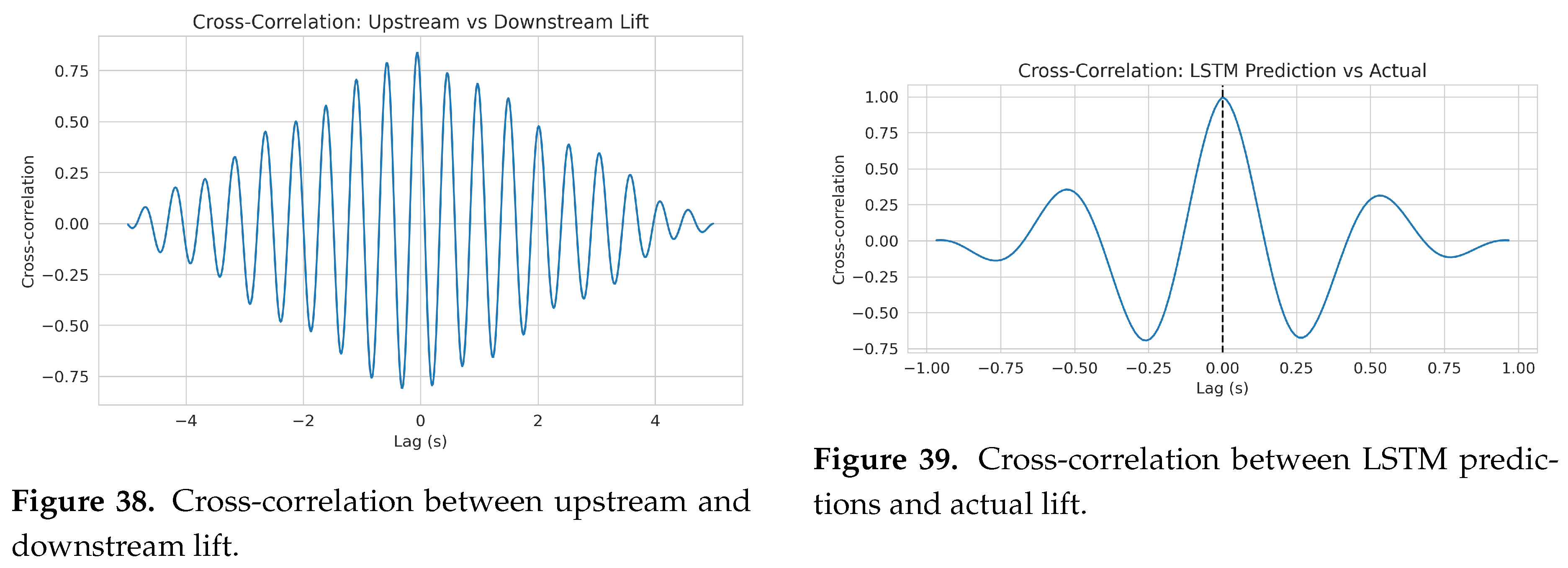
Figure 41.
Extended LSTM forecast of downstream lift (2s beyond CFD data).
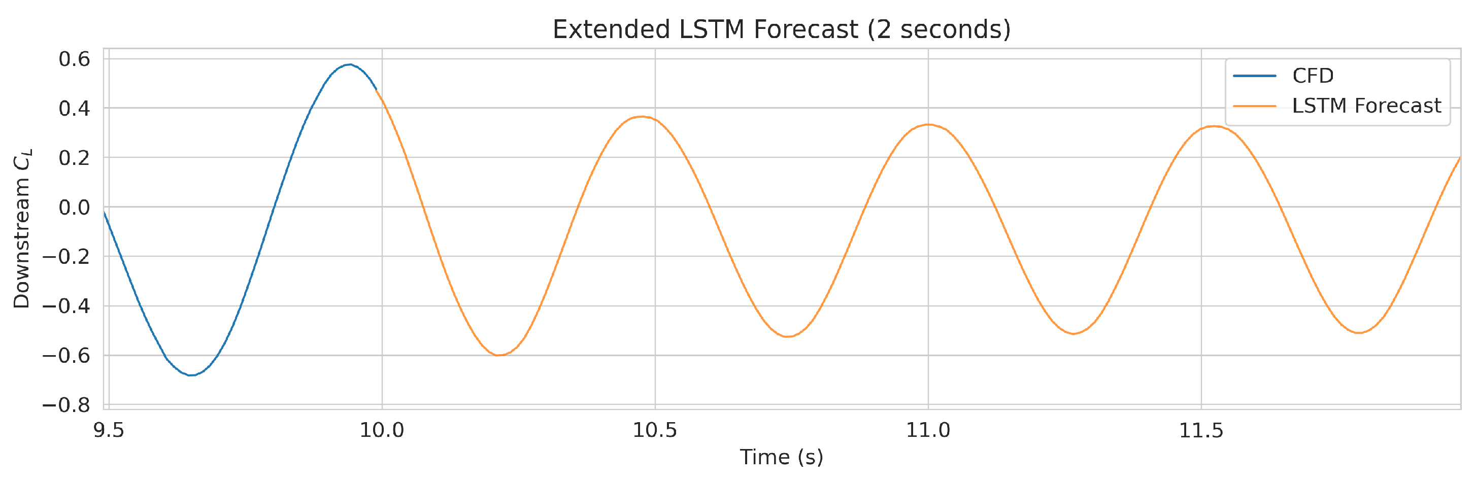
Table 3.
Comparison of force coefficients and Strouhal number for the single-cylinder flow at .
| Quantity | Schäfer and Turek [9] | Present |
|---|---|---|
| Maximum drag coefficient | 3.174 | 3.158 |
| Maximum lift coefficient | 0.964 | 0.782 |
| Strouhal number | 0.300 | 0.262 |
Table 4.
Flow parameters.
| Parameter | Value |
|---|---|
| Freestream velocity (m/s) | 1.0 |
| Kinematic viscosity (m2/s) | (water) |
| Reynolds number | |
| Turbulence intensity at inlet | 5% |
| Time step (s) | 0.001 |
| Total simulation time (s) | 10 |
Table 5.
Time-averaged drag and RMS lift coefficients.
| Cylinder | (RMS) | |
|---|---|---|
| A (upstream) | 0.947 | 0.129 |
| B (downstream) | 0.997 | 0.340 |
Table 6.
Strouhal numbers and shedding frequencies.
| Cylinder | Frequency f (Hz) | Strouhal number |
|---|---|---|
| A (upstream) | 2.041 | 0.204 |
| B (downstream) | 2.041 | 0.306 |
Table 7.
Mean and RMS values at the two probe locations.
| Probe | Location (x, y, z) | Quantity | Mean | RMS |
|---|---|---|---|---|
| 0 | (1.5, 0.2, 0.005) | (m/s) | 0.236 | 0.155 |
| p (Pa) | -0.089 | 0.201 | ||
| 1 | (1.8, 0.2, 0.005) | (m/s) | 0.791 | 0.211 |
| p (Pa) | -0.162 | 0.180 |
Table 8.
Model performance on downstream lift and drag prediction.
| Model | MAE | RMSE | |
|---|---|---|---|
| MLP (lift) | 0.2016 | 0.2493 | 0.4213 |
| LSTM (lift) | 0.0308 | 0.0368 | 0.9895 |
| LSTM (drag) | 0.0102 | 0.0126 | 0.3226 |
| ARIMA (lift) | 0.2125 | 0.2591 | 0.2195 |
Disclaimer/Publisher’s Note: The statements, opinions and data contained in all publications are solely those of the individual author(s) and contributor(s) and not of MDPI and/or the editor(s). MDPI and/or the editor(s) disclaim responsibility for any injury to people or property resulting from any ideas, methods, instructions or products referred to in the content. |
© 2026 by the authors. Licensee MDPI, Basel, Switzerland. This article is an open access article distributed under the terms and conditions of the Creative Commons Attribution (CC BY) license (http://creativecommons.org/licenses/by/4.0/).
Copyright: This open access article is published under a Creative Commons CC BY 4.0 license, which permit the free download, distribution, and reuse, provided that the author and preprint are cited in any reuse.


