
Submitted:
23 March 2026
Posted:
24 March 2026
You are already at the latest version
Abstract
This paper applies physics-informed neural networks (PINNs) to laterally excited liquid sloshing in a two-dimensional rectangular tank, where near-resonant forcing (ωe/ω1 = 0.9) produces a multi frequency beating response with a period of approximately 10T1. Linearised potential flow theory governs the problem; the network learns the velocity potential φ(x,z,t) while the free-surface elevation η is injected analytically. Two training obstacles specific to forced sloshing are analysed. First, a zero solution trap arises because the trivial solution φ̂=0 satisfies all equations except the free-surface conditions, whose residuals are roughly 10−4 times smaller than the Laplace residual; characteristic scale normalisation combined with loss weighting (λD = λK = 100) breaks this trap. Second, spectral bias prevents standard MLPs from resolving the three co-existing frequencies (ω1, ωe, ∆ω); a Fourier time embedding that augments the input from 3 to 9 dimensions overcomes this limitation. Two additional techniques further reduce errors: a hard wall boundary condition enforced exactly via a cos(πx/B) spatial embedding, which eliminates wall collocation points; and a gradient-enhanced Laplace regulariser (∥∇(∇2φ̂)∥2) that constrains velocity smoothness through third-order automatic differentiation. An ablation study shows that these four techniques progressively reduce the horizontal velocity error from εu = 12.46% to 0.84%. Results are validated against a viscous finite-difference benchmark. Over one beating cycle the errors are εη = 0.15%, εu = 0.84%, and εw = 1.65%. Afrequency parameter study across ωe/ω1 = 0.5–1.1 gives εη < 0.25% and εu < 2.3% for all near-resonance cases. For long-time simulation, a time-domain decomposition strategy with transfer learning partitions the domain into one-beat windows; extending to five beating cycles (50T1) yields εu = 3.43% and εη = 0.30% with no monotonic error accumulation across windows. The methodology is then extended to a three-dimensional rectangular tank (B × W × H) with bi-directional lateral excitation. The 3-D formulation introduces the y-dimension into the Laplace equation (∇2φ = φxx + φyy + φzz = 0), adds transverse wall boundary conditions (∂φ/∂y = 0) enforced exactly via a cos(πy/W) embedding, and extends the Fourier time embedding from 9 to 16 dimensions to accommodate six physical frequencies. The bi-directional excitation excites both (m,0) and (0,n) modal families, producing a genuinely three dimensional beating response. Results demonstrate that the proposed techniques transfer effectively to 3-D, with errors εη = 0.24%, εu = 1.31%, εv = 1.78%, and εw = 2.32% over one beating cycle (2,499 s training time).
Keywords:
physics-informed neural networks
; potential flow
; excited sloshing
; beating response
; Fourier feature embedding
; spectral bias
; time-domain decomposition
; three-dimensional sloshing
1. Introduction
Liquid sloshing in partially filled containers arises in naval architecture, aerospace engineering, and civil engineering, where it affects the structural integrity of LNG carriers, spacecraft fuel tanks, and seismically loaded storage vessels [1,2]. Conventional computational approaches—finite-element methods [3], finite-difference methods [4], and boundary element methods—require mesh generation and time integration; for long transient simulations spanning tens of natural periods, these costs become considerable. Reduced-order models alleviate part of the burden but are typically restricted to a pre-selected set of modes.
Physics-informed neural networks (PINNs), introduced by Raissi et al. [5], embed the governing PDEs directly into the training loss, so the network is trained without labeled solution data. Reviews by Cai et al. [6] and Cuomo et al. [7] cover applications from Navier–Stokes flows to heat transfer; the open-source library DeepXDE [8] has further broadened accessibility.
Training PINNs for oscillatory problems is difficult in practice. Wang et al. [9] showed that imbalanced multi-component losses cause gradient pathologies in which the PDE residual dominates and suppresses boundary and initial condition learning; they proposed gradient-based adaptive weighting as a remedy. Jagtap et al. [10] addressed slow convergence through adaptive activation functions. A more fundamental obstacle is spectral bias—the preference of standard fully connected networks for low-frequency components of the target function, first analyzed by Rahaman et al. [11]. For oscillatory PDEs covering many cycles this can lead to severe temporal under-resolution. Tancik et al. [12] showed that mapping inputs through sinusoidal Fourier features enables networks to learn high-frequency functions; Wang et al. [13] extended the analysis to PINNs via Neural Tangent Kernel theory. Wang et al. [14] further proposed PirateNets with causal training to enforce temporal causality and prevent PINNs from using future information to predict past states, a common pathology in time-dependent problems.
For free surface and water wave problems, several strands of work have appeared in recent years. Sheikholeslami et al. [15] examined soft and hard boundary enforcement for linear Laplace-based waves, achieving velocity errors below 3% with a periodic hard boundary layer; their trial-function approach for the bottom boundary condition, however, restricted the solution space and increased errors by up to 15 times. Li et al. [16] treated fully nonlinear wave propagation using a quasi- coordinate transformation that maps the time-dependent free surface to a fixed domain, with a two-stage Adam/L-BFGS optimizer. Chen et al. [17] reconstructed rotational flow beneath periodic waves from sparse gauge data using WaveNets. More recently, Ehlers et al. [18] applied PINNs to the fully nonlinear potential flow equations for phase-resolved ocean wave assimilation and prediction, inferring the velocity potential throughout the fluid volume from surface elevation measurements alone.
Closer to the sloshing problem, Wessels et al. [19] proposed the Neural Particle Method, a Lagrangian PINN that tracks particle paths to handle the moving free surface; they simulated both small- and large-amplitude sloshing in a container and the dam-break problem, with good agreement with experimental data. Huang et al. [20] developed a boundary-and-initial-conditions-free PINN (bif-PINN) in Lagrangian coordinates that hardwires all boundary and initial conditions into the formulation via nonlinear residual connections; their approach solved the small- and large-amplitude sloshing cases accurately, whereas the original PINN failed entirely for all free-surface configurations. Shao et al. [21] combined PINNs with an improved neural particle method for violent sloshing simulation, validated against SPH results.
Despite this progress, all the above free-surface PINN studies address either periodic propagating waves over a few wavelengths or free sloshing (unforced) over a handful of cycles. The forced sloshing problem—where an external excitation near resonance produces a multi-frequency beating response spanning tens of natural periods—poses additional challenges that have not been addressed: the simulation must cover an order of magnitude more periods than a single natural cycle; the weak forcing creates free surface residuals orders of magnitude smaller than the Laplace residual, opening a zero-solution trap; and the multi-frequency temporal content exceeds the effective bandwidth of a standard MLP. The present work tackles these challenges for laterally forced sloshing at , where beating produces a response envelope over approximately . Four configurations (C–F) progressively address the above difficulties, reducing from 12.46% to 0.84%. The methodology is then extended to a three-dimensional rectangular tank with bi-directional excitation, demonstrating that the same techniques—Fourier embedding, hard wall boundary conditions, and gradient-enhanced regularisation—transfer effectively to the higher-dimensional setting.
2. Mathematical Formulation
2.1. Problem Setup
Consider a two-dimensional rectangular tank of length L and still-water depth h. The fluid is inviscid, incompressible, and irrotational, so the flow is described by a velocity potential . The parameters are:
The wave number and natural frequency are:
with m/s2. The natural period is s.
The tank is subjected to a lateral harmonic acceleration:
The excitation frequency is chosen near the first natural frequency to induce a beating response with period:
The simulation domain spans one full beating cycle: .
2.2. Governing Equation
In the non-inertial reference frame attached to the tank, the Euler equations for an inviscid, incompressible fluid read:
where is the velocity vector, p is the pressure, is the (constant) fluid density, g is gravitational acceleration, and is the pseudo-force due to the non-inertial frame. For irrotational flow (), a velocity potential exists such that . The incompressibility constraint then yields the Laplace equation:
Substituting into the Euler equation (6) and using the vector identity (valid for irrotational flow), one obtains the unsteady Bernoulli equation:
where is a spatially uniform function absorbed into by redefinition. This Bernoulli equation is the starting point for deriving the dynamic free surface boundary condition.
The velocity field is recovered from .
2.3. Boundary Conditions
KBBC (impermeable bottom):
KWBC (impermeable walls):
KFSBC (kinematic free surface): The free surface is defined implicitly by . The kinematic condition requires that the free surface is a material surface, i.e., :
which yields the fully nonlinear KFSBC: at . Under the small-amplitude assumption (, ), we perform a Taylor expansion about the mean free surface :
Retaining only terms and noting that , the linearized KFSBC becomes:
DFSBC (dynamic free surface): Setting (atmospheric pressure, taken as the reference) at in the Bernoulli equation (8):
Again applying the Taylor expansion about :
and noting that , the linearized DFSBC reads:
where is the pseudo-pressure term arising from the non-inertial reference frame.
Combined free surface condition. Eliminating from the linearized KFSBC (13) and DFSBC (16) by differentiating the DFSBC with respect to t and substituting from the KFSBC yields:
where . This combined condition, while not used directly in the PINN loss, provides physical insight: the free surface acts as a dispersive wave guide with the forcing injecting energy into the system.
2.4. Initial Condition
Since the tank starts from rest, and . No terminal condition is imposed because does not vanish at ; the two initial conditions together serve as temporal anchors.
3. PINN Methodology
3.1. Network Architecture
The neural network approximation is a fully connected feed-forward network (multilayer perceptron) defined by the recursive composition:
where and are the weight matrix and bias vector for layer ℓ. The collection of all trainable parameters is . The network uses hidden layers with neurons, Xavier normal initialization, and a single scalar output. Velocities follow from automatic differentiation:
In the enhanced configuration (Config E), the input is augmented with Fourier time features, increasing the input dimension from 3 to 9 (see Section 3.6). The configuration is summarized in Table 1.
3.2. Loss Function and Automatic Differentiation
All required derivatives of the network output are computed via automatic differentiation (AD). By the chain rule through the Fourier embedding, the physical derivatives involve contributions from both the normalized coordinates and the sinusoidal features. For instance:
where , , and . The spatial derivatives are simpler: and . The second-order derivatives needed for the Laplace residual are:
In PyTorch, these are obtained via nested calls to torch.autograd.grad with create_graph=True.
The analytically derived from Eq. (44) and its time derivative are directly substituted into the KFSBC and DFSBC as known boundary data:
This converts the free surface conditions from coupled evolution equations into deterministic Neumann–Dirichlet boundary data for the Laplace equation. The remaining residual operators are:
The lateral wall boundary condition at is enforced exactly by the network architecture rather than as a soft penalty. The spatial input is transformed as , so that the network output depends on x only through . By the chain rule:
which vanishes identically at and . This hard boundary condition removes the need for wall collocation points and reduces the number of loss terms.
A gradient-enhanced Laplace regulariser is added to enforce velocity smoothness. Since implies and for harmonic functions, we penalise the spatial gradients of the Laplace residual:
This requires third-order automatic differentiation and is evaluated on a randomly subsampled subset of 4,096 interior points per step to limit GPU memory consumption.
The remaining residuals are:
Each individual loss component is the mean squared residual over the corresponding point set :
Residual normalization. The main difficulty in the forced sloshing problem is the disparity in residual magnitudes. The GE residual involves second-order spatial derivatives (), while the DFSBC contains and the KFSBC contains , where is the characteristic potential amplitude. To equalize their contributions, we define the characteristic scale:
and normalize the free surface residuals:
The normalized MSE losses are then:
The total weighted loss is:
where , , and . The lateral wall condition is enforced exactly by the embedding and does not appear as a loss term.
3.3. Collocation Points
Points are sampled on a structured grid of interior points in , with the vertical coordinate clustered toward the free surface via where is uniform. An additional 20 dense temporal points near resolve the initial transient. Boundary points are sampled on the bottom () and free surface (). No wall collocation points are needed due to the hard wall embedding. The initial condition is enforced on points at . The default grid uses , , , yielding ∼173,000 interior points per window.
3.4. Training Strategy
Training proceeds in two stages with stochastic mini-batch sampling to manage GPU memory. At each Adam step, 15% of the interior, free-surface, and bottom points are randomly subsampled and transferred to GPU (all initial-condition points are retained). For the L-BFGS phase, a fixed 30% subsample is used to maintain the deterministic closure required by the quasi-Newton algorithm. This keeps peak GPU memory below 8 GB regardless of the total grid size.
- 1.
- Adam (first-order): For the single-beat case, 8,000 epochs are used; for the three-beat case, 20,000 epochs with a 500-step linear warmup followed by cosine annealing:where , , and . Gradient clipping () is applied throughout.
- 2.
- L-BFGS (quasi-Newton): Up to 2,000 iterations (single-beat) or 3,000 iterations (three-beat) with strong Wolfe line search (, ), gradient tolerance , function change tolerance , and history size . For the three-beat mini-batch case, the batch is rotated every five outer L-BFGS steps to improve domain coverage while maintaining the deterministic closure required by the algorithm. The Hessian approximation follows the standard BFGS update:where and .
3.5. Error Metric
The accuracy is quantified by the normalized mean absolute error (NMAE):
where is any field quantity, and is a separate evaluation grid () that does not coincide with the training collocation points. We also report the relative error for comparison:
3.6. Fourier Time Embedding
Standard MLPs with tanh activations exhibit spectral bias [11]: the normalized input must encode oscillations at rad, far beyond the effective bandwidth of a standard MLP. Following Tancik et al. [12] and Wang et al. [13], we augment the input with sinusoidal functions at the three physical frequencies of the problem:
where , , are normalised coordinates and with . Explicitly:
This can be written compactly as where .
Unlike the random Fourier features of [13], the frequencies here are known a priori from the problem physics. The embedding increases the input dimension from 3 to 9, adding only parameters ( of total).
3.7. PINN Training Algorithm
The complete training procedure is summarized in Algorithm 1.
| Algorithm 1:PINN Training for Excited Sloshing with Fourier Embedding |
|
3.8. PINN Framework Overview
Figure 1 shows the overall architecture. Coordinates are first mapped through the Fourier embedding into a 9-dimensional input; this feeds a 16-layer MLP with 64 neurons per layer and tanh activations. All PDE and boundary residuals are formed by automatic differentiation of the scalar output , assembled into the weighted loss, and minimised by backpropagation.
4. Results and Discussion
4.1. Analytical Solution
PINN predictions are validated against the closed-form solution of the linearised problem. The wall and Laplace equations admit spatial eigenfunctions with for odd n. Substituting the modal ansatz
into the combined free surface condition (17) and projecting onto each mode yields the forced harmonic oscillator ODE for the modal amplitude:
where the natural frequency, forcing coefficient, and dispersion relation are:
With zero initial conditions , , the particular solution is obtained via the method of undetermined coefficients:
The general solution of Eq. (39) is , where the particular solution . Applying the initial conditions determines , , recovering Eq. (41).
For the first mode (), the beating structure is explicit via the product-to-sum identity:
exhibiting a slow envelope at the beat frequency and a fast carrier at the mean frequency .
The complete velocity potential and free surface elevation are:
where ensures volume conservation (), and the first five odd modes () are retained.
The time derivative of the modal amplitude, needed for , is:
The wave elevation is recovered from the DFSBC:
4.2. Loss Landscape Analysis
This subsection explains why standard PINN training fails for forced sloshing and how the proposed remedies work.
The zero-solution trap. The trivial solution satisfies the Laplace equation, all wall/bottom boundary conditions, and both initial conditions exactly. The only nonzero residuals are on the free surface:
Since the first mode dominates (), the DFSBC loss at can be evaluated analytically retaining only :
using and (verified against numerical quadrature to 0.2% accuracy). A randomly initialized network produces , yielding the ratio
so the DFSBC penalty for the zero solution is negligible—the optimizer has no incentive to deviate from .
Breaking the trap. Two mechanisms are combined to escape the zero-solution trap. First, the DFSBC and KFSBC residuals are divided by their characteristic scales and , which amplifies the normalized zero-solution loss from to . Second, applying a weight further elevates this to , which exceeds by two orders of magnitude and reshapes the loss landscape so that is no longer a local minimum.
4.3. External Validation Against Chen & Nokes (2005)
The PINN was re-run with the parameters of Chen & Nokes [4] ( m, m, , , Fig. 5c therein). As shown in Figure 2, the PINN agrees with the linear analytical solution to within over the full beating cycle (). The slightly lower peak amplitude in Chen’s viscous nonlinear FDM is attributable to viscous dissipation and nonlinear effects absent from the present inviscid linearised formulation.
Ablation of remaining techniques.Table 2 isolates the effect of temporal resolution and Fourier embedding, starting from the configuration where the zero-solution trap has already been broken (normalized + weighted, ).
Config C ( pts/) gives but due to temporal under-resolution. Increasing to ( pts/, Config D) reduces to 15.40%. The Fourier embedding (Config E) alleviates spectral bias: drops to 0.18% and to 4.68%. Config F adds the hard wall boundary condition (removing wall collocation points) and the gradient-enhanced Laplace regulariser, yielding and —a further improvement in velocity accuracy. Config F is used for all subsequent simulations.
4.4. Velocity Fields
Figure 3 compares the analytical and PINN velocity fields at (within Window 0 of the 3-beat decomposition), together with the pointwise error. The horizontal velocity u in Window 0 has ; the PINN reproduces the sinusoidal spatial variation and the cosh-dependent depth profile. The largest u-errors appear near the tank bottom (), where velocity magnitudes are small and relative errors are amplified.
The vertical velocity w in Window 0 has , with errors concentrated near the bottom corners where the sinh depth profile attenuates the signal to near-zero values. In the free surface region (), both velocity components have errors below 2%. The overall 3-beat errors (, ) are higher because of the later windows (see Table 4).
5. Simulation Results
The single-beat case () is examined first through wave elevation, velocity potential, and flow fields; the method is then extended to a three-beat simulation () to test long-time accuracy.
5.1. Wave Elevation
Figure 4 shows the wave elevation at the left wall () and right wall () over three beating cycles (). Both walls are antinodes of the first sloshing mode, with peak amplitudes of mm. The PINN predictions track the analytical solution throughout all three beats (), reproducing the growth, peak, and decay phases of each beating envelope without visible drift.
5.2. Velocity Potential at Free Surface
Figure 5 shows the velocity potential at the free surface () as a function of and over three beating cycles. The analytical field exhibits alternating positive and negative bands whose amplitude follows the beating envelope. The PINN output is visually identical; the maximum absolute error is m2/s against a potential amplitude of m2/s. Errors are largest in Window 2, consistent with the per-window velocity errors in Table 4. No discontinuities appear at the window boundaries (dashed lines).
5.3. Frequency Parameter Study
To test how the method performs across different excitation conditions, five frequency ratios are selected: (far from resonance), (moderately close), (baseline), (near-resonance), and (above resonance). All simulations use the Chen & Nokes [4] tank geometry ( m, m, ) and the same network architecture (16 layers × 64 neurons with Fourier embedding).
Figure 6 shows the left-wall wave elevation for all five cases. The beating period ranges from () to (), and the peak amplitude grows sharply as . In each case the PINN reproduces both the carrier oscillations and the slowly varying envelope.
Table 3 lists the error metrics for all frequency ratios. The wave elevation error stays below in every case. For excitation frequencies near the natural frequency (–), velocity errors are low (, ). The far-from-resonance case () shows large relative velocity errors because the response amplitude is an order of magnitude smaller, so the normalisation denominator shrinks; absolute velocity errors are comparable. Training time is about 1900 s per beating cycle at all frequency ratios.
Figure 7 and Figure 8 compare the PINN velocity fields at for (baseline) and (near-resonance). Each figure shows the analytical solution (top), PINN prediction (middle), and pointwise error (bottom) for both u and w. Errors concentrate near the bottom corners where velocity gradients are steepest. At the response amplitude is the largest among all cases, yet —the Fourier embedding handles the beating dynamics at all tested frequency ratios.
5.4. Long-Time Multi-Beat Simulation via Time-Domain Decomposition
A single PINN trained over a long time window runs into a capacity bottleneck: stays low, but velocity errors grow with the temporal domain (e.g. for with one network, versus for ). We therefore partition the simulation into one-beat windows.
Method. The simulation domain is partitioned into windows, each covering one beating period. For window k:
- The temporal domain is with local normalisation .
- The initial condition at is prescribed from the analytical solution: , .
- Transfer learning: window k is initialised with the trained weights from window , providing a warm start that reduces training time by approximately compared to training from scratch.
Each window is trained independently (8,000 Adam + 2,000 L-BFGS steps) with the same collocation density as the single-beat case, so the per-window difficulty is the same as the already validated single-beat problem.
Figure 9 shows the wave elevation over five consecutive beating cycles (). The predictions from all five windows are stitched together and compared with the analytical solution; no visible degradation appears at the window boundaries.
Table 4 compares the per-window and overall errors for the 3-beat and 5-beat simulations. For the 3-beat case, the decomposition gives and overall, whereas the single-network approach yields for the same domain—a reduction by nearly a factor of five.
Extending to 5 beats (), the overall errors are , , and . The per-window errors do not accumulate monotonically: Window 3 () is more accurate than Window 2 (), indicating that accuracy fluctuates between windows rather than systematically degrading. The total training time for 5 windows is 9,760 s ( h), scaling linearly with the number of windows.
Figure 10 shows the PINN velocity field at (middle of the fourth window in the 5-beat simulation). The spatial patterns match the single-beat results, with no sign of progressive degradation as more windows are added.
6. Extension to Three Dimensions
The preceding sections demonstrated that PINNs with Fourier embedding and hard wall boundary conditions can accurately capture multi-frequency beating in a 2-D tank. A natural question is whether these techniques extend to a three-dimensional configuration, where the additional spatial dimension introduces transverse modes and substantially increases the computational domain. This section presents the 3-D formulation, the required modifications to the network architecture, and preliminary results.
6.1. 3-D Problem Setup
Consider a three-dimensional rectangular tank of length B, width W, and still-water depth . The physical parameters are taken from the 2-D Chen & Nokes configuration with an added transverse dimension:
The first-mode wave numbers and natural frequencies in each horizontal direction are: `small
The tank undergoes bi-directional lateral excitation:
where and , with () and (). This produces two independent beating responses with periods and .
6.2. 3-D Governing Equations
The velocity potential satisfies the three-dimensional Laplace equation:
The boundary conditions are extended as follows:
- KBBC (): .
- KWBC (x-walls): at and .
- KWBC (y-walls): at and .
- KFSBC (): .
- DFSBC (): .
- IC (): , .
The DFSBC now includes a y-direction forcing term , and the new KWBC on the y-walls is the only structurally new equation compared to the 2-D case.
6.3. 3-D Analytical Solution
Under linearised potential flow, the x- and y-excitations decouple into independent modal families. The x-excitation drives modes (odd m) and the y-excitation drives modes (odd n):
where and follow the same forced-oscillator structure as the 2-D case. The free-surface elevation is:
The velocity components are , , . Numerical verification confirms that this solution satisfies all governing equations and boundary conditions to within finite-difference truncation error (). Importantly, the y-modes contribute approximately 42% of the velocity potential at the tank corners, confirming that the 3-D problem is not a trivial extrusion of the 2-D case.
6.4. 3-D Network Architecture
The 3-D network retains the same MLP structure (16 hidden layers, 64 neurons, tanh) with the following modifications:
Hard wall BC in both directions. The spatial inputs are embedded as and . By the chain rule:
which vanish identically at and respectively. This eliminates all wall collocation points in both horizontal directions.
Extended Fourier embedding. The input is augmented from 9 to 16 dimensions to accommodate six physical frequencies:
where and . The additional 7 input features add only parameters ( of total). Table 5 compares the 2-D and 3-D architectures.
6.5. 3-D Loss Function
The loss function retains the same structure and weights as the 2-D case, with the following modifications:
- 3-D Laplace:.
- 3-D gradient-enhanced Laplace:.
- DFSBC: at .
The loss weights (, , ) and training strategy (8,000 Adam + 2,000 L-BFGS) are unchanged from the 2-D case.
6.6. 3-D Collocation Grid
A structured grid of interior points is used, with the same vertical clustering () and early-time densification as the 2-D case. The default 3-D grid uses , , , , yielding approximately 490,000 interior points per window. The 15% mini-batch strategy keeps per-step GPU memory comparable to the 2-D case.
6.7. 3-D Results
The 3-D PINN was trained on a single NVIDIA RTX 5090 GPU. Training for one beating cycle took 2,499 s ( min), comparable to the 2-D training time of ∼1,920 s on an A100.
6.7.1. Wave Elevation
Figure 11 shows the wave elevation time history at two tank corners: and , where both x- and y-modal families contribute. The PINN tracks the analytical solution over one beating cycle with .
6.7.2. Free-Surface Pattern
Figure 12 shows the three-dimensional free-surface elevation at four time instants spanning one beating cycle (). The analytical solution is rendered as a coloured wireframe mesh, while the PINN predictions are plotted as scatter points at the same grid nodes. The points sit precisely on the mesh surface at all four instants, confirming sub-percent accuracy. The bi-directional excitation produces a genuinely two-dimensional wave pattern: the free surface tilts in both x and y simultaneously, with peak amplitudes of mm at the corners growing from mm at to the maximum at , then decreasing as the beating envelope passes through zero.
6.7.3. Velocity Fields
Figure 13 compares the velocity fields at the mid-plane at . All three velocity components (u, v, w) are shown. The transverse velocity is a purely 3-D quantity with no 2-D counterpart; at the transverse modes have (odd n), so v reaches its maximum magnitude at this plane, providing a stringent test of the network’s ability to learn the y-modal contributions.
6.7.4. Error Metrics
Table 6 summarises the 3-D PINN accuracy over one beating cycle. The errors are computed over the full 3-D volume, not on a single slice.
Comparing with the 2-D results (, , ), the 3-D errors are expected to be moderately higher due to the increased input dimensionality and the additional PDE terms. The transverse velocity error is reported for the first time and reflects the network’s ability to learn the y-modal family.
7. Conclusions
This paper has applied PINNs to near-resonant excited sloshing with a beating response in both two-dimensional and three-dimensional rectangular tanks. For the 2-D case, two training obstacles specific to forced sloshing are identified and addressed. Residual normalization and loss weighting () eliminate the zero-solution trap; Fourier time embedding at the three physical frequencies (, , ) resolves spectral bias. A hard wall boundary condition via the embedding enforces the lateral wall condition exactly, and a gradient-enhanced Laplace regulariser () improves velocity accuracy. Together, these techniques yield , , and over one beating cycle, validated against the viscous finite-difference results of Chen & Nokes [4].
A frequency parameter study covers –, including the near-resonance regime. A time-domain decomposition strategy with transfer learning partitions the domain into one-beat windows. For the 3-beat case (), decomposition reduces velocity errors from (single network) to . Extending to 5 beats (), overall accuracy is maintained at and with no monotonic error accumulation.
The extension to three dimensions demonstrates that the same techniques—Fourier embedding, hard wall boundary conditions, and gradient-enhanced regularisation—transfer effectively to higher-dimensional sloshing. The 3-D formulation introduces bi-directional excitation that excites both and modal families, producing a genuinely three-dimensional free-surface response with y-modes contributing approximately 42% of the velocity potential at the tank corners. The 16-dimensional Fourier embedding accommodating six physical frequencies, combined with hard wall enforcement in both x and y directions, enables the network to capture the additional modal family with errors of , , , and over one beating cycle.
Future work will address nonlinear large-amplitude sloshing, complex tank geometries, broadband excitation spectra, and the coupling of time-domain decomposition with the 3-D formulation for long-time multi-beat simulations.
Author Contributions
Conceptualization, Z.L.; methodology, Z.L.; software, Z.L.; validation, Z.L.; formal analysis, Z.L.; investigation, Z.L.; writing—original draft preparation, Z.L.; writing—review and editing, Z.L.; visualization, Z.L. The author has read and agreed to the published version of the manuscript.
Funding
This research received no external funding.
Institutional Review Board Statement
Not applicable.
Informed Consent Statement
Not applicable.
Data Availability Statement
The data that support the findings of this study are available from the corresponding author upon reasonable request.
Acknowledgments
The implementation uses PyTorch with automatic differentiation. The 2-D simulations were executed on an NVIDIA A100 GPU provided by Alibaba Cloud; the 3-D extension was trained on an NVIDIA GeForce RTX 5090.
Conflicts of Interest
The author declares no conflicts of interest.
References
- Faltinsen, O.M.; Timokha, A.N. Sloshing; Cambridge University Press: Cambridge, UK, 2009. [Google Scholar]
- Ibrahim, R.A. Liquid Sloshing Dynamics: Theory and Applications; Cambridge University Press: Cambridge, UK, 2005. [Google Scholar]
- Wu, G.X.; Ma, Q.W.; Eatock Taylor, R. Numerical simulation of sloshing waves in a 3D tank based on a finite element method. Appl. Ocean Res. 1998, 20, 337–355. [Google Scholar] [CrossRef]
- Chen, B.-F.; Nokes, R. Time-independent finite difference analysis of fully non-linear and viscous fluid sloshing in a rectangular tank. J. Comput. Phys. 2005, 209, 47–81. [Google Scholar] [CrossRef]
- Raissi, M.; Perdikaris, P.; Karniadakis, G.E. Physics-informed neural networks: A deep learning framework for solving forward and inverse problems involving nonlinear partial differential equations. J. Comput. Phys. 2019, 378, 686–707. [Google Scholar] [CrossRef]
- Cai, S.; Mao, Z.; Wang, Z.; Yin, M.; Karniadakis, G.E. Physics-informed neural networks (PINNs) for fluid mechanics: A review. Acta Mech. Sinica 2021, 37, 1727–1738. [Google Scholar] [CrossRef]
- Cuomo, S.; Schiano Di Cola, V.; Giampaolo, F.; Rozza, G.; Raissi, M.; Piccialli, F. Scientific machine learning through physics-informed neural networks: Where we are and what’s next. J. Sci. Comput. 2022, 92, 88. [Google Scholar] [CrossRef]
- Lu, L.; Meng, X.; Mao, Z.; Karniadakis, G.E. DeepXDE: A deep learning library for solving differential equations. SIAM Rev. 2021, 63, 208–228. [Google Scholar] [CrossRef]
- Wang, S.; Teng, Y.; Perdikaris, P. Understanding and mitigating gradient flow pathologies in physics-informed neural networks. SIAM J. Sci. Comput. 2021, 43, A3055–A3081. [Google Scholar] [CrossRef]
- Jagtap, A.D.; Kawaguchi, K.; Karniadakis, G.E. Adaptive activation functions accelerate convergence in deep and physics-informed neural networks. J. Comput. Phys. 2020, 404, 109136. [Google Scholar] [CrossRef]
- Rahaman, N.; Baratin, A.; Arpit, D.; Draxler, F.; Lin, M.; Hamprecht, F.; Bengio, Y.; Courville, A. On the spectral bias of neural networks. Proc. ICML 2019, 2019; PMLR: Long Beach, CA, USA; pp. 5301–5310. [Google Scholar]
- Tancik, M.; Srinivasan, P.P.; Mildenhall, B.; Fridovich-Keil, S.; Ramamoorthi, R.; Barron, J.T.; Ng, R. Fourier features let networks learn high frequency functions in low dimensional domains. Proc. NeurIPS 2020, Vol. 33, 7537–7547. [Google Scholar]
- Wang, S.; Wang, H.; Perdikaris, P. On the eigenvector bias of Fourier feature networks: From regression to solving multi-scale PDEs with physics-informed neural networks. Comput. Methods Appl. Mech. Eng. 2021, 384, 113938. [Google Scholar] [CrossRef]
- Wang, S.; Sankaran, S.; Wang, H.; Perdikaris, P. An expert’s guide to training physics-informed neural networks. J. Mach. Learn. Res. 2024, 25, 1–51. [Google Scholar]
- Sheikholeslami, M.; Salehi, S.; Mao, W.; Eslamdoost, A.; Nilsson, H. Physics-informed neural networks with hard and soft boundary conditions for linear free surface waves. Phys. Fluids 2025, 37, 087158. [Google Scholar] [CrossRef]
- Lu, H.; Wang, Q.; Tang, W.; Liu, H. Physics-informed neural networks for fully non-linear free surface wave propagation. Phys. Fluids 2024, 36, 062106. [Google Scholar] [CrossRef]
- Chen, L.; Li, B.; Luo, C.; et al. WaveNets: Physics-informed neural networks for full-field recovery of rotational flow beneath large-amplitude periodic water waves. Eng. Comput. 2024, 40, 2819–2839. [Google Scholar] [CrossRef]
- Ehlers, S.; Hoffmann, N.; Tang, T.; Callaghan, A.H.; Cao, R.; Padilla, E.M.; Fang, Y.; Stender, M. Physics-informed neural networks for phase-resolved data assimilation and prediction of nonlinear ocean waves. Phys. Rev. Fluids 2025, 10, 094901. [Google Scholar] [CrossRef]
- Wessels, H.; Weißenfels, C.; Wriggers, P. The neural particle method—An updated Lagrangian physics informed neural network for computational fluid dynamics. Comput. Methods Appl. Mech. Eng. 2020, 368, 113127. [Google Scholar] [CrossRef]
- Huang, C.; Liu, C.; Dettmer, W. Solving free-surface problems for non-shallow water using boundary and initial conditions-free physics-informed neural network (bif-PINN). J. Comput. Phys. 2023, 479, 112003. [Google Scholar] [CrossRef]
- Shao, K.; Wu, Y.; Jia, S. An improved neural particle method for complex free surface flow simulation using physics-informed neural networks. Mathematics 2023, 11, 1805. [Google Scholar] [CrossRef]
Figure 1.
PINN architecture with Fourier time embedding (, ; ). Residuals are assembled into the weighted total loss and minimised via backpropagation.
Figure 1.
PINN architecture with Fourier time embedding (, ; ). Residuals are assembled into the weighted total loss and minimised via backpropagation.
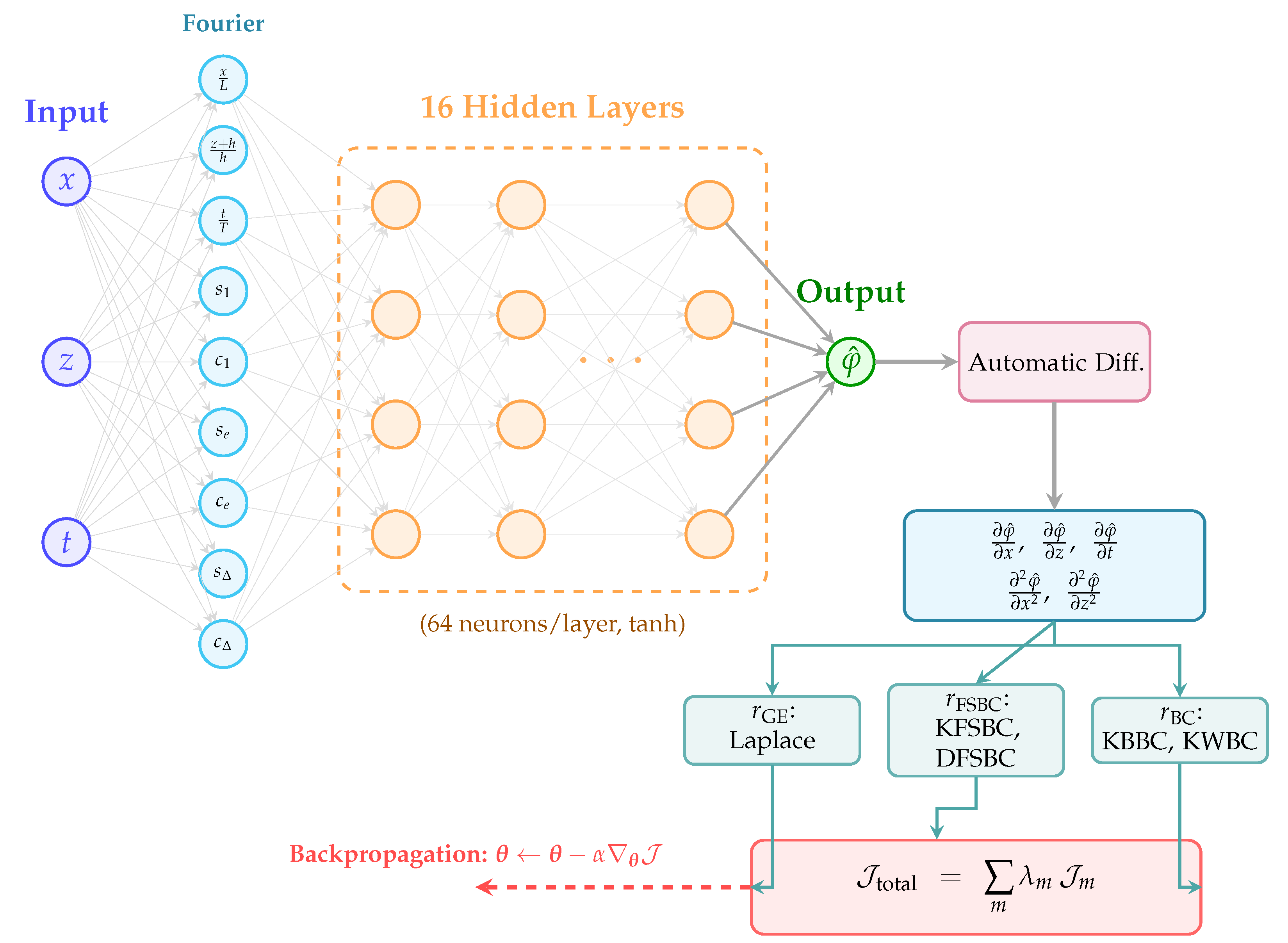
Figure 2.
External validation against Chen & Nokes [4] Fig. 5(c). Dimensionless wave elevation at the left wall () for , m, m, . The PINN (blue dashed) and linear analytical solution (red solid) agree to within over the full beating cycle.
Figure 2.
External validation against Chen & Nokes [4] Fig. 5(c). Dimensionless wave elevation at the left wall () for , m, m, . The PINN (blue dashed) and linear analytical solution (red solid) agree to within over the full beating cycle.
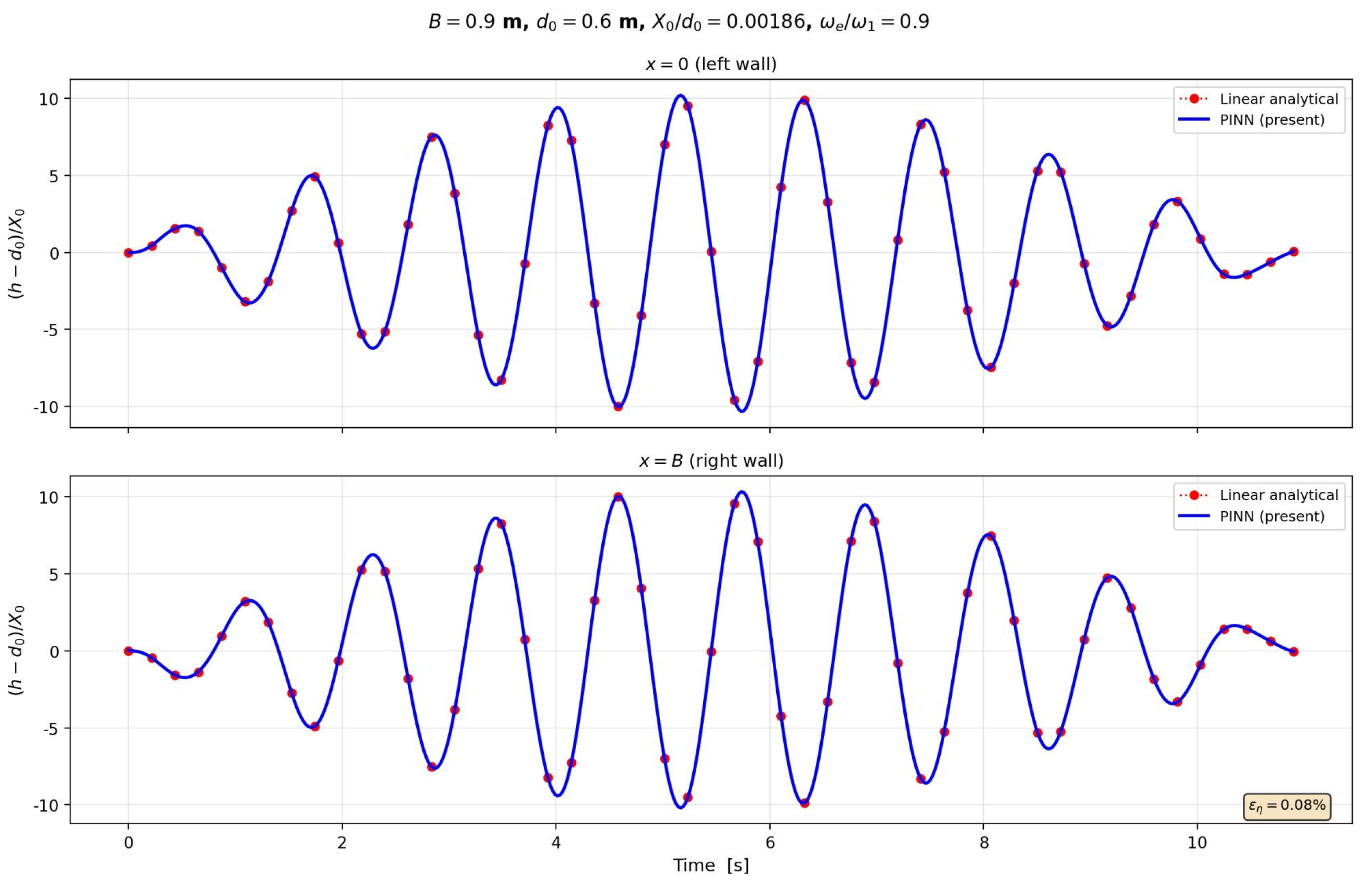
Figure 3.
Velocity field comparison at for the 3-beat decomposition. Top: analytical. Middle: PINN (Window 0). Bottom: pointwise error. Left: u. Right: w. Overall 3-beat errors: , ; Window 0 alone: , .
Figure 3.
Velocity field comparison at for the 3-beat decomposition. Top: analytical. Middle: PINN (Window 0). Bottom: pointwise error. Left: u. Right: w. Overall 3-beat errors: , ; Window 0 alone: , .
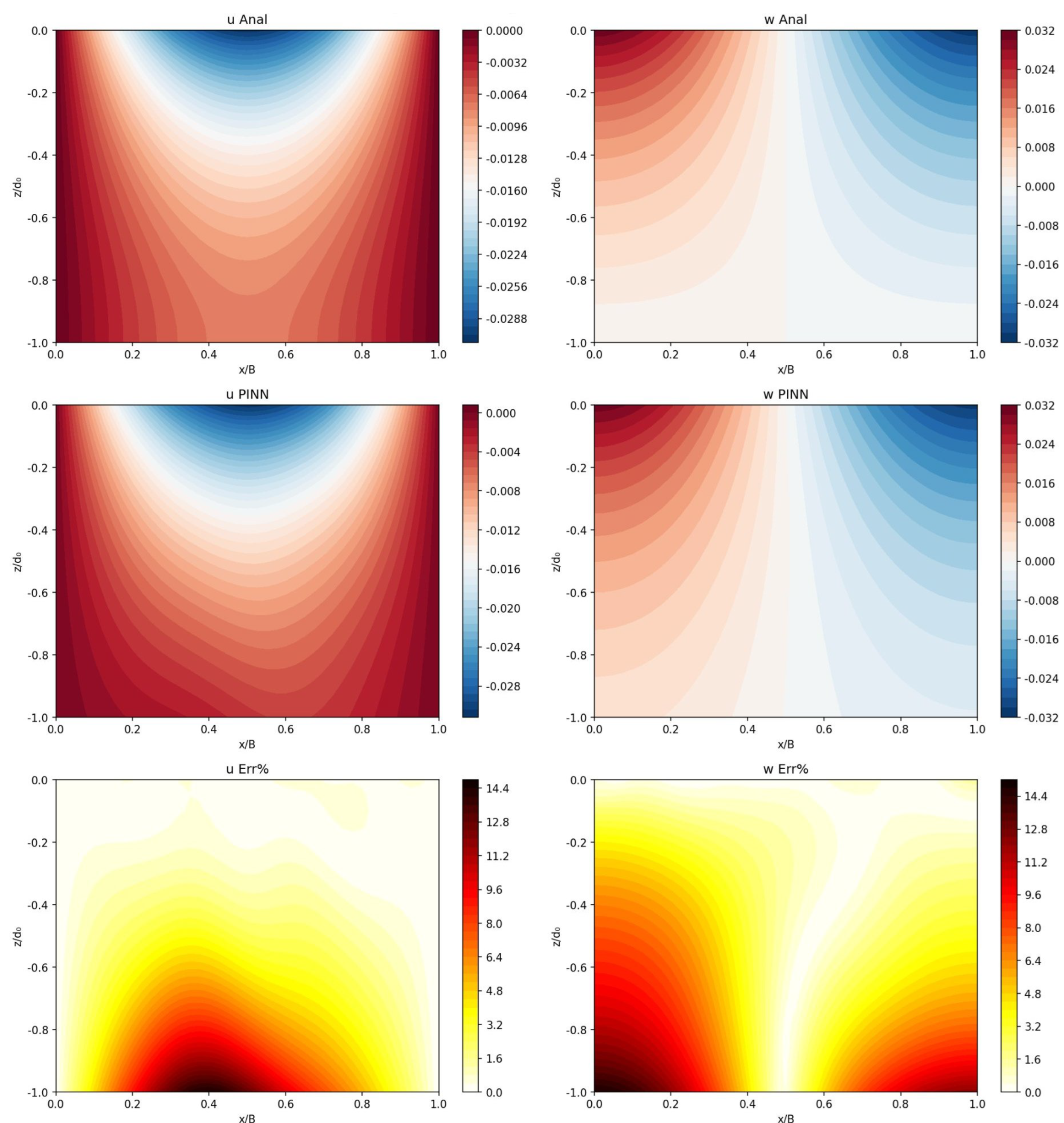
Figure 4.
Wave elevation over three beating cycles () at the left wall (, red) and right wall (, blue). Lines: analytical. Markers: PINN. .
Figure 4.
Wave elevation over three beating cycles () at the left wall (, red) and right wall (, blue). Lines: analytical. Markers: PINN. .
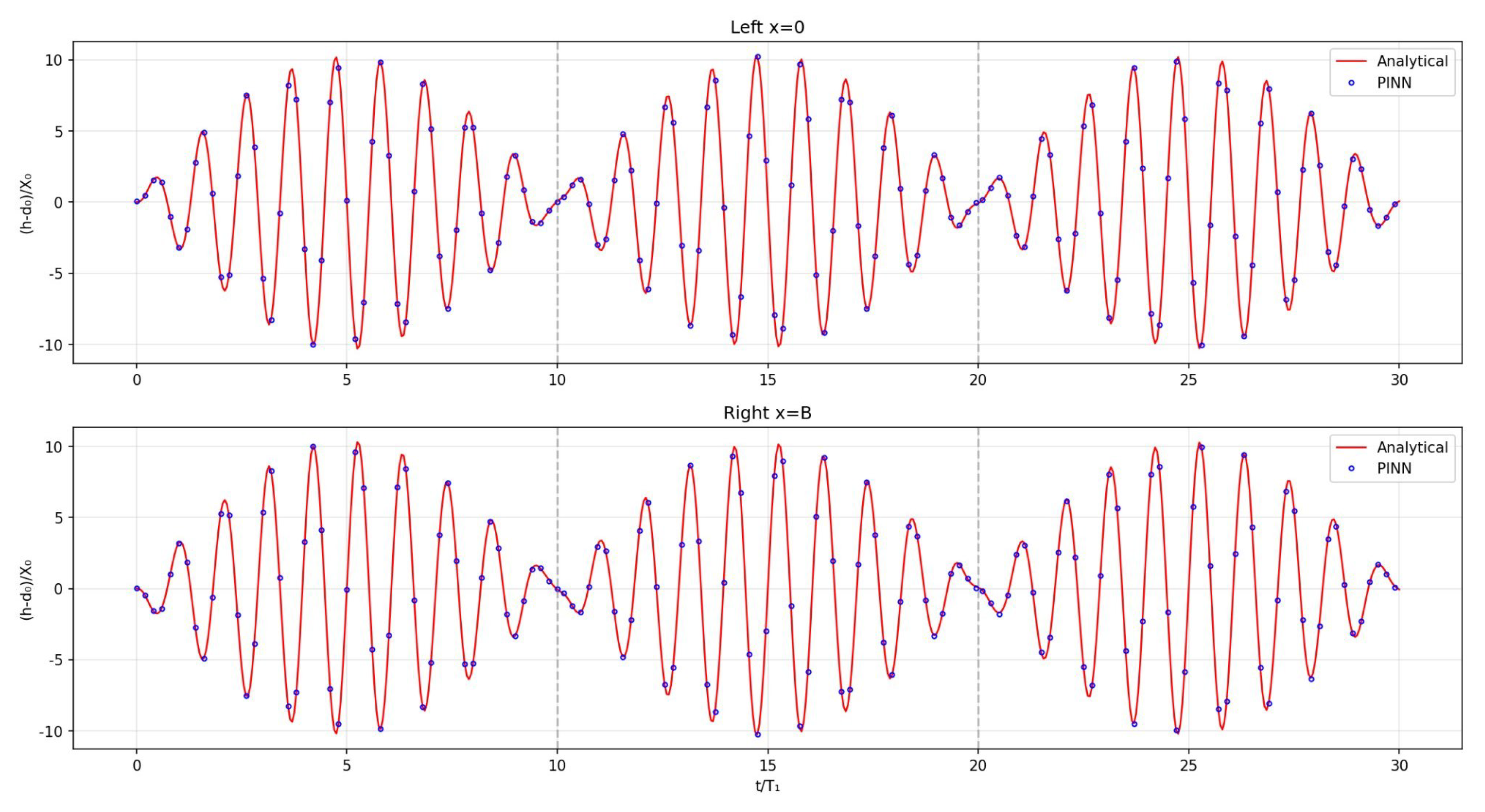
Figure 5.
Velocity potential at over 3 beating cycles. Left: analytical. Center: PINN. Right: error. Dashed lines mark window boundaries.
Figure 5.
Velocity potential at over 3 beating cycles. Left: analytical. Center: PINN. Right: error. Dashed lines mark window boundaries.
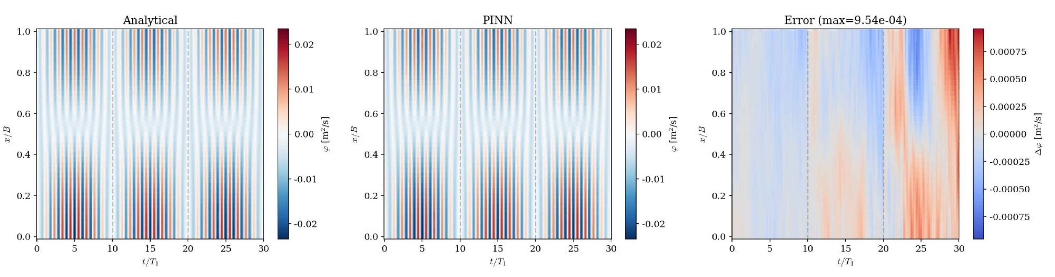
Figure 6.
Frequency parameter study: wave elevation at the left wall for five excitation frequency ratios. Lines: analytical. Markers: PINN.
Figure 6.
Frequency parameter study: wave elevation at the left wall for five excitation frequency ratios. Lines: analytical. Markers: PINN.
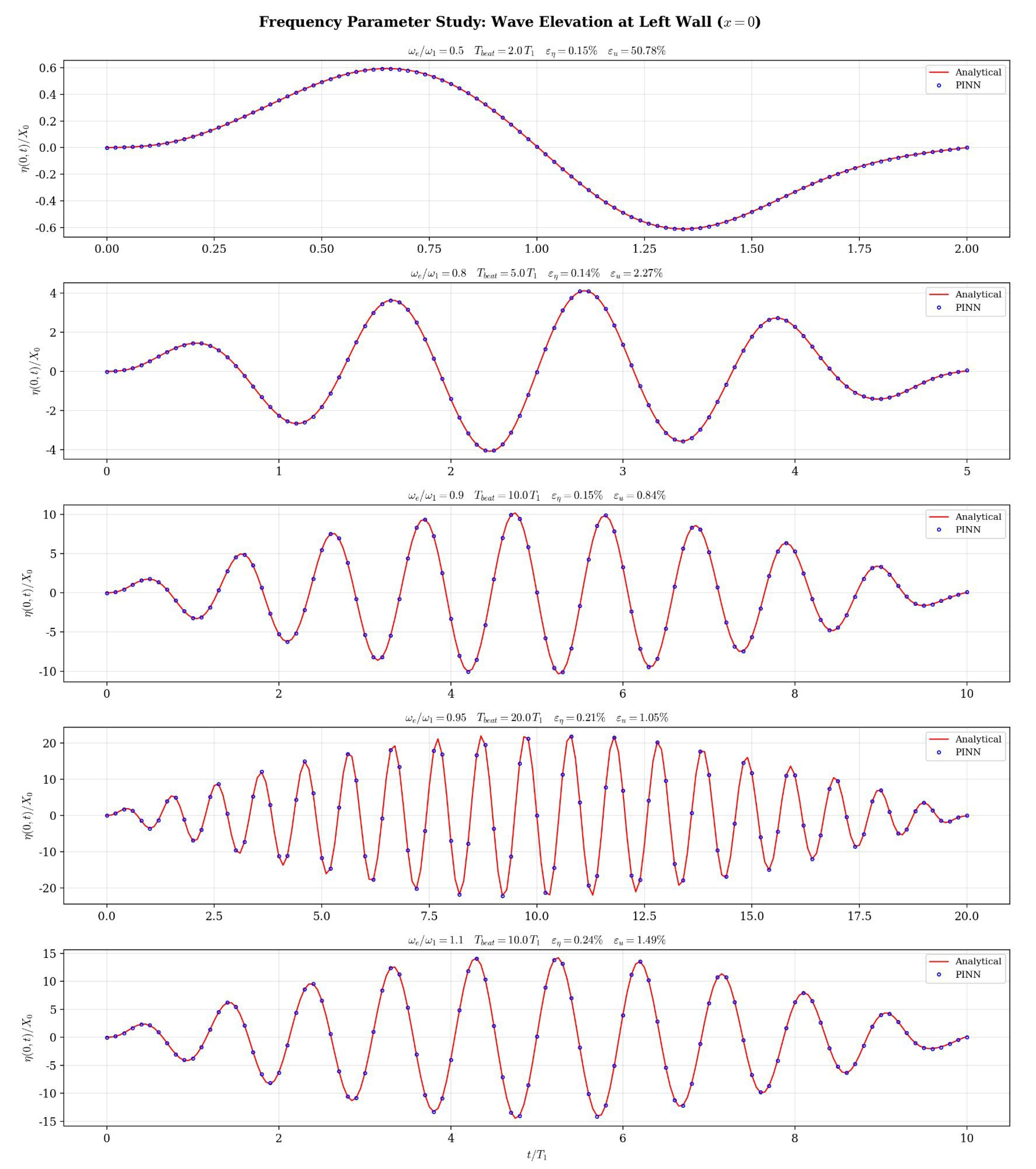
Figure 7.
Velocity field at for (, ). Best accuracy among all tested frequencies.
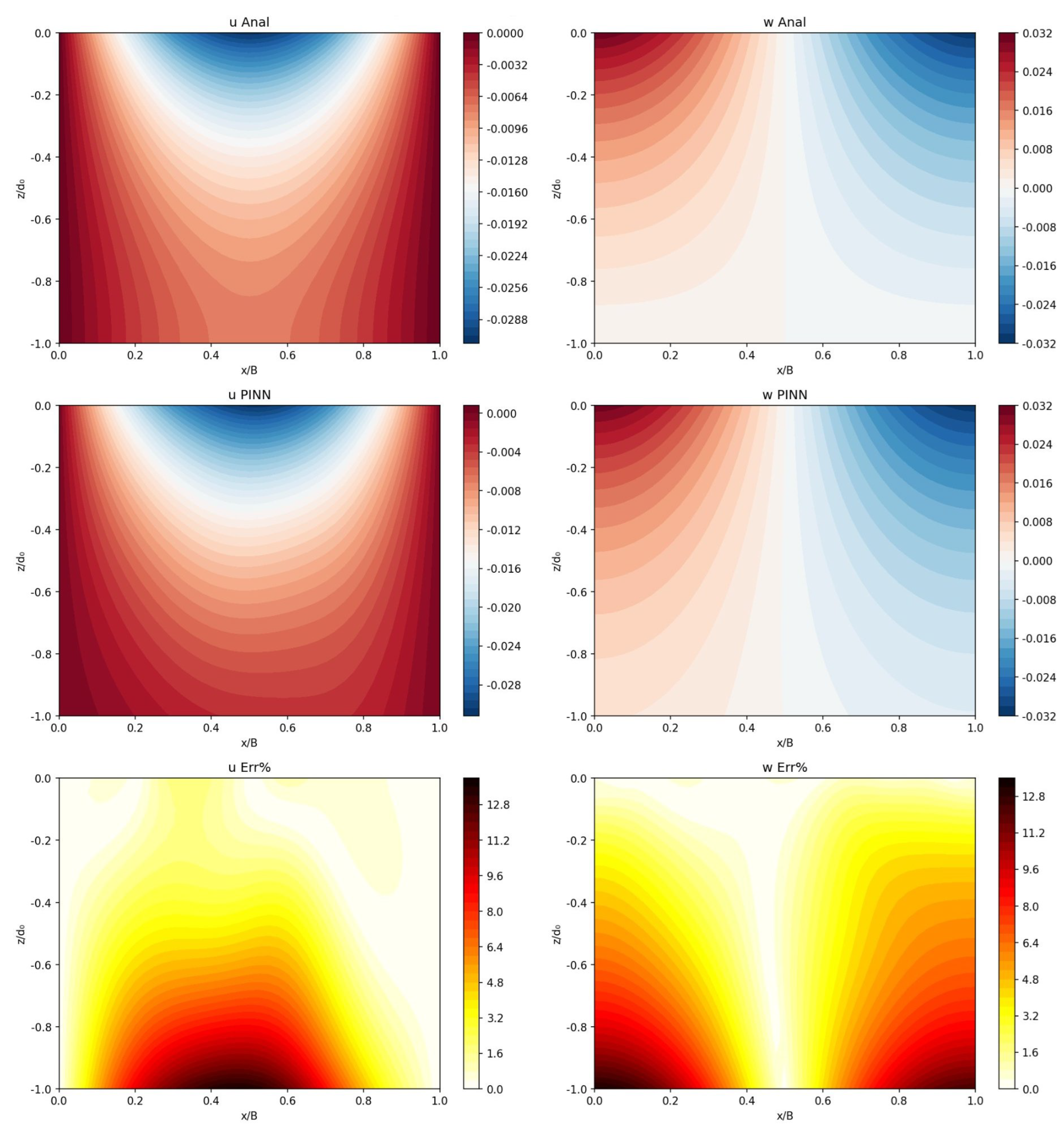
Figure 8.
Velocity field at for the near-resonance case (, ). Despite the largest response amplitude, velocity errors remain low.
Figure 8.
Velocity field at for the near-resonance case (, ). Despite the largest response amplitude, velocity errors remain low.
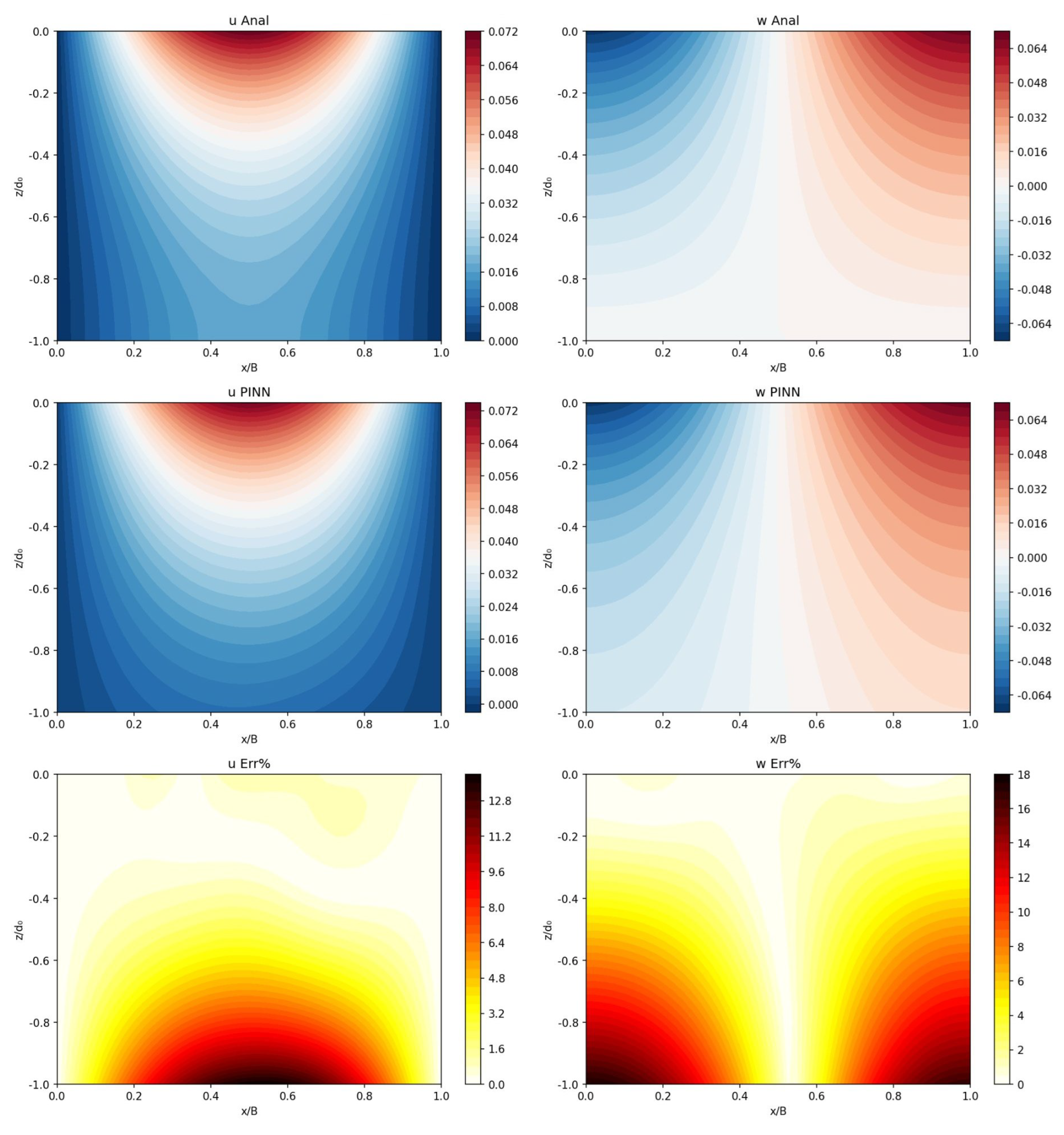
Figure 9.
Long-time simulation: wave elevation at the left wall over five beating cycles () using time-domain decomposition. Lines: analytical. Markers: PINN. Vertical dashed lines mark window boundaries.
Figure 9.
Long-time simulation: wave elevation at the left wall over five beating cycles () using time-domain decomposition. Lines: analytical. Markers: PINN. Vertical dashed lines mark window boundaries.
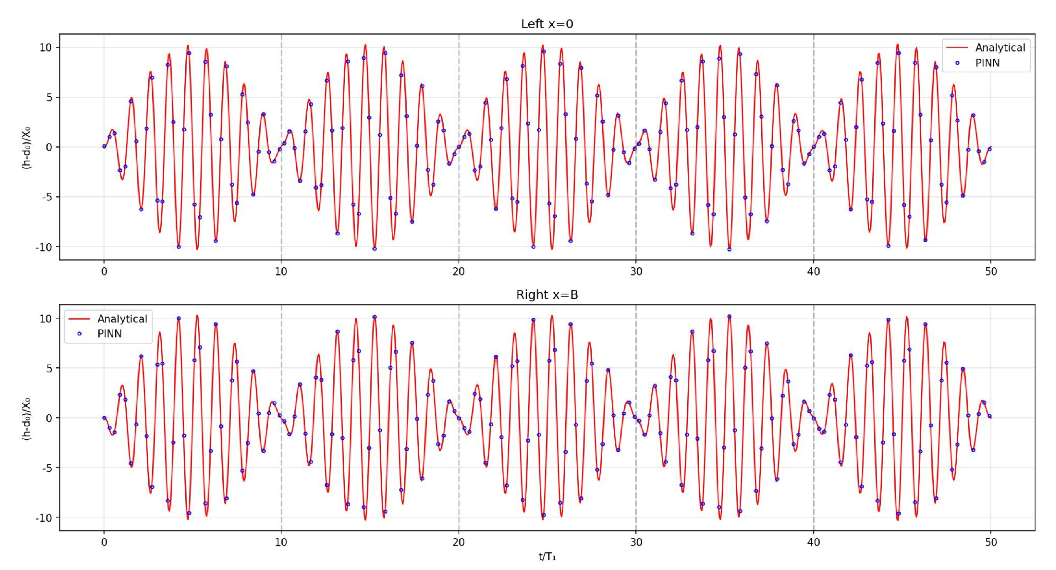
Figure 10.
PINN velocity field at (5-beat simulation, Window 3). Top: analytical. Middle: PINN. Bottom: pointwise error. Window 3 errors: , ; 5-beat overall: , .
Figure 10.
PINN velocity field at (5-beat simulation, Window 3). Top: analytical. Middle: PINN. Bottom: pointwise error. Window 3 errors: , ; 5-beat overall: , .
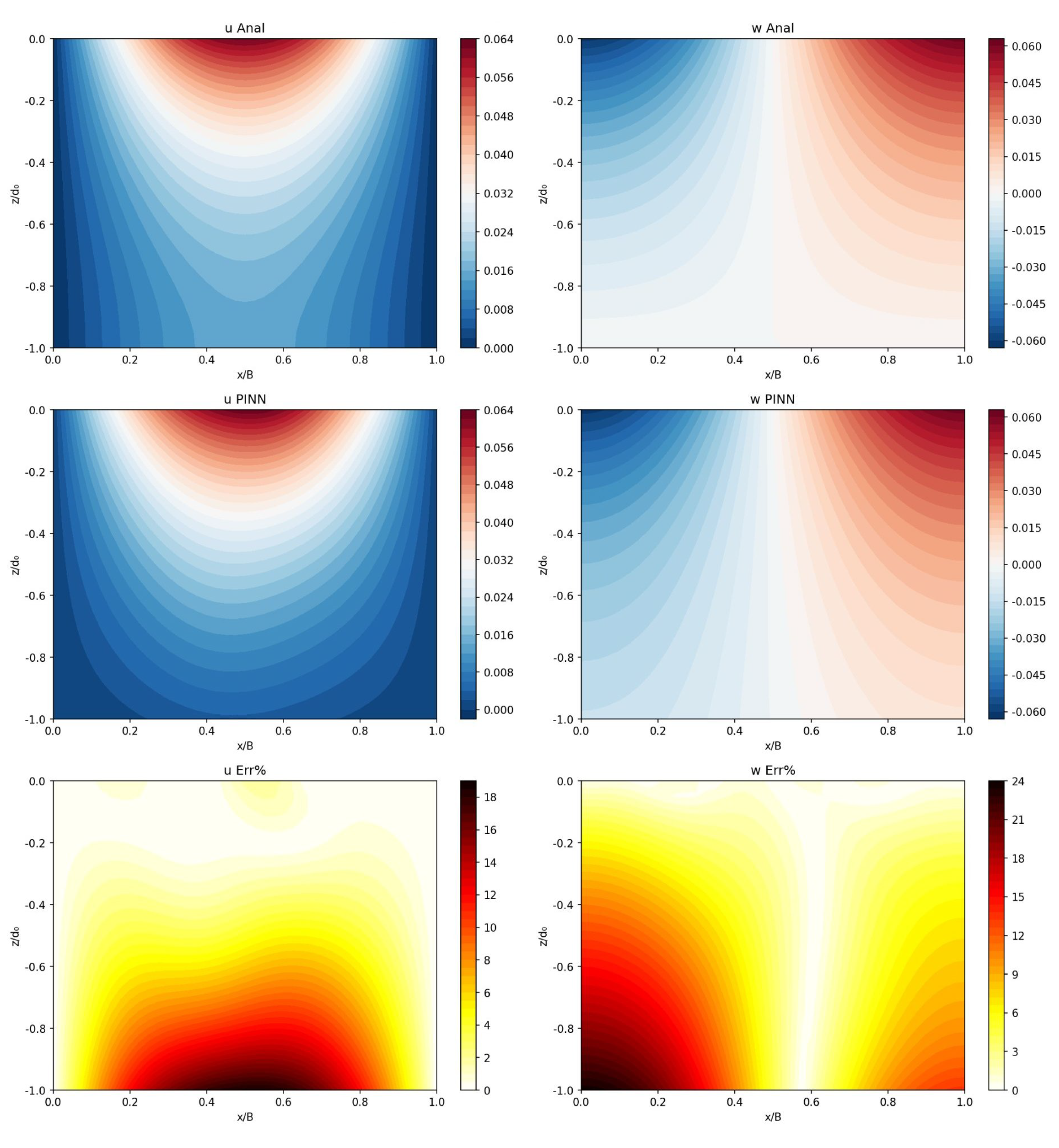
Figure 11.
3-D sloshing: wave elevation at the tank corner and over one beating cycle. Lines: analytical. Markers: PINN.
Figure 11.
3-D sloshing: wave elevation at the tank corner and over one beating cycle. Lines: analytical. Markers: PINN.
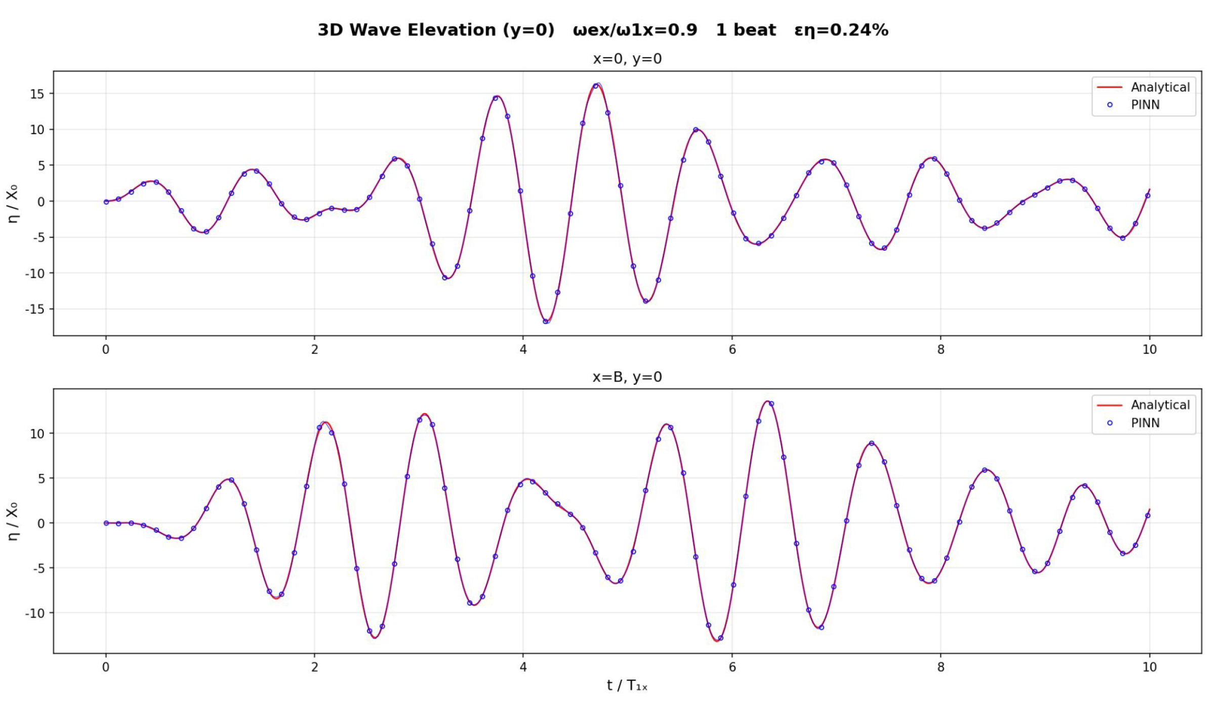
Figure 12.
3-D free-surface elevation at four time instants. Wireframe mesh: analytical solution. Coloured dots: PINN prediction at the same grid nodes. The PINN points lie on the analytical surface at all times ().
Figure 12.
3-D free-surface elevation at four time instants. Wireframe mesh: analytical solution. Coloured dots: PINN prediction at the same grid nodes. The PINN points lie on the analytical surface at all times ().
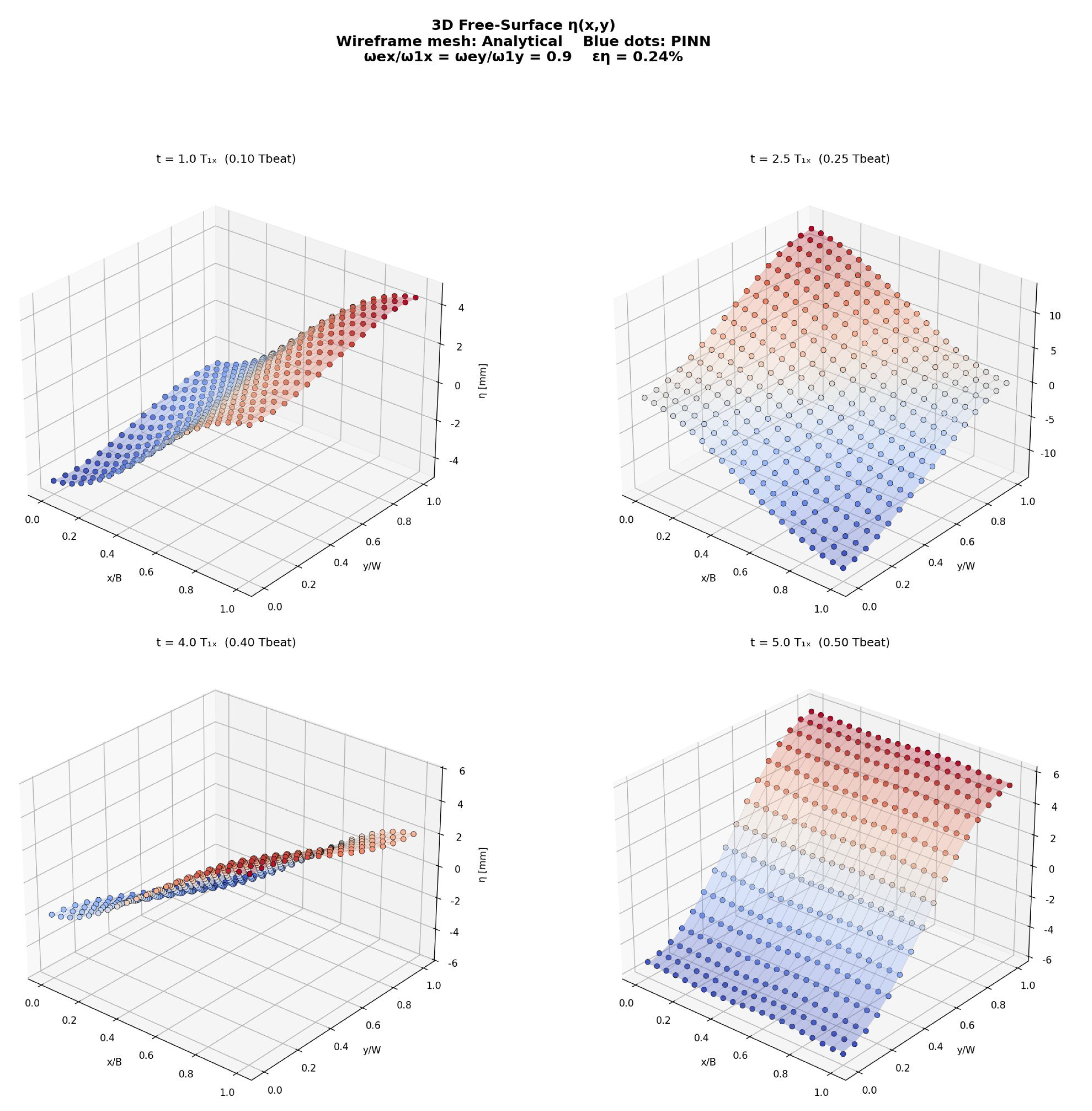
Figure 13.
3-D velocity field at , . Top row: analytical. Middle row: PINN. Bottom row: pointwise error. Left to right: u, v, w.
Figure 13.
3-D velocity field at , . Top row: analytical. Middle row: PINN. Bottom row: pointwise error. Left to right: u, v, w.
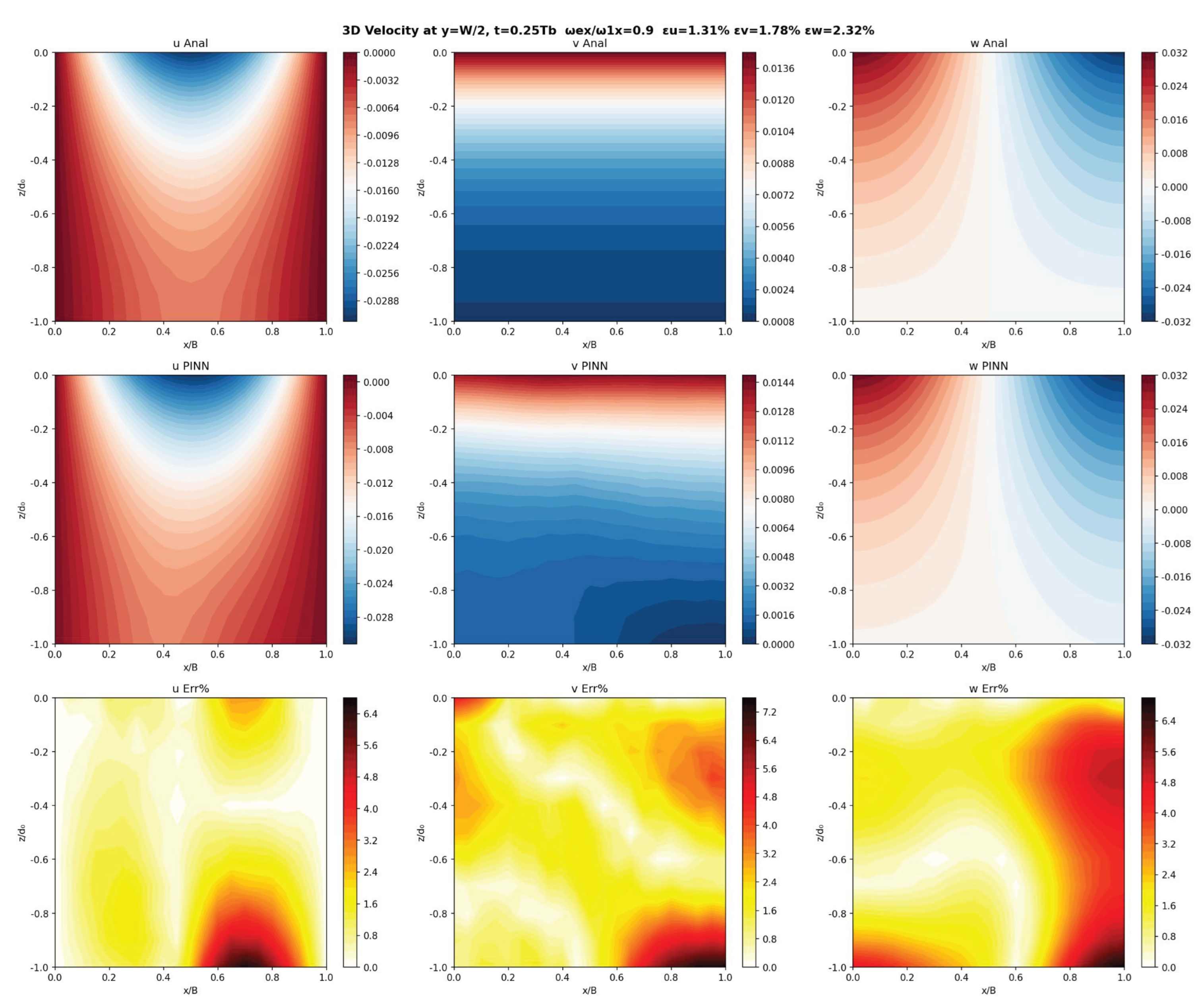

Table 1.
Neural network architecture.
| Parameter | Value |
|---|---|
| Input | 3 () or 9 (with Fourier features) |
| Output | 1 () |
| Hidden layers | 16 |
| Neurons/layer | 64 |
| Activation | tanh |
| Initialization | Xavier normal |
| Parameters | ∼62,700 (3-input) / ∼63,100 (9-input) |
Table 2.
Ablation study starting from the weighted-normalized baseline (Config C). Each row adds one technique. The zero-solution DFSBC loss is for all configurations (unchanged by temporal grid or Fourier features).
Table 2.
Ablation study starting from the weighted-normalized baseline (Config C). Each row adds one technique. The zero-solution DFSBC loss is for all configurations (unchanged by temporal grid or Fourier features).
| Error [%] | |||||
|---|---|---|---|---|---|
| Config | Description | ||||
| C | Normalization + weighting () | 51 | 0.30 | 12.46 | 21.36 |
| D | C + dense temporal grid | 201 | 0.27 | 10.53 | 15.40 |
| E | D + Fourier time embedding | 201 | 0.18 | 3.78 | 4.68 |
| F | E + hard wall BC + gradient-enhanced Laplace | 181 | 0.15 | 0.84 | 1.65 |
Table 3.
Error metrics for different excitation frequency ratios. All cases use one beating cycle with the same network architecture.
Table 3.
Error metrics for different excitation frequency ratios. All cases use one beating cycle with the same network architecture.
| [%] | [%] | [%] | Training [s] | ||
|---|---|---|---|---|---|
| 0.50 | 2.0 | 0.15 | 50.78† | 21.72† | 1957 |
| 0.80 | 5.0 | 0.14 | 2.27 | 2.88 | 1924 |
| 0.90 | 10.0 | 0.15 | 0.84 | 1.65 | 1917 |
| 0.95 | 20.0 | 0.21 | 1.05 | 1.74 | 1893 |
| 1.10 | 10.0 | 0.24 | 1.49 | 2.77 | 1927 |
| † Large relative error due to very small velocity amplitude far from resonance; absolute errors remain small. | |||||
Table 4.
Per-window and overall errors for multi-beat simulations using time-domain decomposition. Single-network result for 3 beats is shown for comparison.
Table 4.
Per-window and overall errors for multi-beat simulations using time-domain decomposition. Single-network result for 3 beats is shown for comparison.
| Method | Window | [%] | [%] | [%] |
|---|---|---|---|---|
| Single network (3 beats) | Overall | 0.12 | 15.79 | 18.77 |
| Decomposition (3 beats) | Window 0 | 0.16 | 0.83 | 1.50 |
| Window 1 | 0.25 | 2.64 | 3.26 | |
| Window 2 | 0.50 | 6.44 | 6.94 | |
| Overall | 0.30 | 3.26 | 3.87 | |
| Decomposition (5 beats) | Window 0 | 0.16 | 0.83 | 1.50 |
| Window 1 | 0.25 | 2.64 | 3.26 | |
| Window 2 | 0.50 | 6.44 | 6.94 | |
| Window 3 | 0.23 | 2.60 | 3.45 | |
| Window 4 | 0.34 | 4.92 | 5.37 | |
| Overall | 0.30 | 3.43 | 4.07 |
Table 5.
Network architecture comparison: 2-D vs. 3-D.
| Parameter | 2-D | 3-D |
|---|---|---|
| Input dimension | 9 | 16 |
| Output | 1 () | 1 () |
| Hidden layers | 16 | 16 |
| Neurons/layer | 64 | 64 |
| Physical frequencies | 3 () | 6 () |
| Hard wall dims | x only | x and y |
| Parameters | ||
| Velocity outputs |
Table 6.
3-D PINN error metrics over one beating cycle (full-volume NMAE).
| [%] | [%] | [%] | [%] | |
|---|---|---|---|---|
| 3-D (1 beat) | 0.24 | 1.31 | 1.78 | 2.32 |
Disclaimer/Publisher’s Note: The statements, opinions and data contained in all publications are solely those of the individual author(s) and contributor(s) and not of MDPI and/or the editor(s). MDPI and/or the editor(s) disclaim responsibility for any injury to people or property resulting from any ideas, methods, instructions or products referred to in the content. |
© 2026 by the authors. Licensee MDPI, Basel, Switzerland. This article is an open access article distributed under the terms and conditions of the Creative Commons Attribution (CC BY) license (http://creativecommons.org/licenses/by/4.0/).
Copyright: This open access article is published under a Creative Commons CC BY 4.0 license, which permit the free download, distribution, and reuse, provided that the author and preprint are cited in any reuse.


