
Submitted:
20 March 2026
Posted:
23 March 2026
You are already at the latest version
Abstract
To address the challenges of high miss detection rates and accuracy degradation in UAV-based insulator defect detection—primarily stemming from complex background interference and the loss of fine-grained features—this paper presents an optimized lightweight detection framework based on an improved YOLOv8 model. The integration of a Spatial-to-Depth Convolution (SPDConv) module strengthens the extraction of fine-grained features for microscopic defects, while the incorporation of an SCConv module suppresses computational redundancy, leading to a 2.80\% accuracy improvement. This architecture is further enhanced by a Channel and Spatial Reconstruction Attention Module (CSRAM), which dynamically prioritizes target-related regions and mitigates noise from vegetation and infrastructure. To improve regression robustness against low-quality annotations and blurred boundaries, a Focal-WIoU loss function utilizing a dynamic non-monotonic focusing mechanism is introduced. Experimental results on complex insulator datasets demonstrate that the proposed model achieves an mAP@0.5 of 91.75\%, a 4.40\% increase over the YOLOv8 baseline, effectively enabling precise multi-scale defect recognition under extreme operational conditions.
Keywords:
insulators
; object detection
; SPDConv
; YOLOv8 algorithm
; WIoU
1. Introduction
Transmission lines constitute the backbone of modern energy infrastructure, where insulators serve a critical dual role in providing mechanical support and electrical isolation. Within the framework of data-driven power system maintenance, the automated identification of insulator defects (such as breakages, pollution, and missing fittings) via Unmanned Aerial Vehicles (UAVs) has emerged as a significant research frontier [1,2,3,4]. From the perspective of computer vision and mathematical optimization, these detection tasks can be characterized as high-dimensional non-linear feature extraction and regression problems under non-stationary noise conditions. While single-stage detectors like the YOLO series [5,6,7] have balanced speed and accuracy in general contexts, their performance often deteriorates when confronted with the extreme scale variations and complex backgrounds inherent in power line imagery [8,9].
A fundamental mathematical challenge in current deep learning architectures is the preservation of information entropy during the feature downsampling process. Traditional convolutional neural networks (CNNs) rely heavily on strided convolutions or pooling layers to reduce computational complexity; however, these operations inherently discard fine-grained spatial details. For microscopic defect types—such as missing tie wires—which occupy only a fraction of the total pixels, this information loss leads to a failure in convergence toward the global optimum [10]. Furthermore, the presence of metallic transmission towers and dense vegetation introduces significant high-frequency noise, which often overwhelms the subtle feature signatures of the targets [11]. Effective feature representation, therefore, requires a mechanism that can distinguish salient information from redundant background noise without sacrificing the integrity of the data stream.
Another critical bottleneck lies in the loss function design for bounding box regression. In real-world UAV inspection datasets, variables such as variable lighting and perspective distortion often result in “noisy labels,” where manual annotations exhibit significant positional shifts or blurred boundaries. Standard Intersection over Union (IoU) based loss functions treat all samples with uniform priority, making the model overly sensitive to these low-quality outliers during gradient descent. This sensitivity hinders the generalization performance of the detector, particularly in extreme working conditions where the defect edges are poorly defined. Optimization of the regression target through a dynamic re-weighting mechanism is thus essential to ensure stable convergence and high localization precision.
To address these issues, this paper proposes an optimized YOLOv8 framework. The primary contributions are summarized as follows:
- 1.
- We introduce a Spatial-to-Depth Convolution (SPDConv) module to replace traditional strided convolutions, mapping spatial information into the channel dimension to minimize the loss of fine-grained features essential for tiny defect detection.
- 2.
- A Channel and Spatial Reconstruction Attention Module (CSRAM) is designed to re-weight feature maps in both spatial and channel dimensions, effectively decoupling target features from complex background noise.
- 3.
- We propose the Focal-WIoU loss function, which incorporates a dynamic non-monotonic focusing mechanism to evaluate the outlier degree of samples, thereby reducing the influence of low-quality annotations on the regression task.
- 4.
- Extensive experimental validation on a large-scale power grid dataset confirms the superior robustness and accuracy of the proposed model in multi-scale insulator defect recognition.
2. Insulator Recognition Based on Improved YOLOv8
2.1. Spatial-to-Depth Convolution Module
In the context of UAV-based transmission line inspections, complex background interference (e.g., vegetation and buildings), extreme scale variations, and diverse lighting conditions introduce massive amounts of noise into high-definition aerial images, thereby significantly increasing the difficulty of detecting tiny insulator defects. In traditional convolutional neural network configurations, the inclusion of strided convolution operations and pooling layers for feature downsampling reduces the computational burden but inevitably discards complex details within the images. In particular, when processing microscopic defects (such as missing tie wires and subtle breakages) that occupy only a tiny fraction of pixels in aerial images, the loss of fine-grained key features caused by downsampling operations becomes a particularly severe problem. This severely weakens the network’s capability to learn the local texture features of defects, ultimately resulting in frequent miss detections and degraded detection performance. To address this issue, this paper introduces a novel Spatial-to-Depth Convolution (SPDConv) module to replace the strided convolutions and pooling layers in traditional convolutional networks. It demonstrates superior performance over conventional deep learning models in the tasks of processing small objects and retaining fine-grained features [12].
Based on the CNN architecture, SPDConv employs a spatial-to-depth (SPD) convolutional layer and a non-strided convolution (Non-strided-Conv) layer to replace traditional strided convolution and pooling operations. This design effectively retains all information within the channel dimension, thereby avoiding the degradation of feature representation and overcoming the model performance limitations caused by the loss of fine-grained feature information in traditional convolutional neural network architectures. The SPD layer enhances feature representation by mapping the spatial dimension of the input feature map to the channel dimension while preserving its intra-channel information. To mitigate the possibility of oversampling by the SPD layer, the Conv layer utilizes standard convolution operations to convolve each feature map, retaining its fine-grained information. Figure 1 illustrates the SPDConv operation when the scale is equal to 2.
In Figure 1, (a) represents an arbitrary original feature map; (b), (c), and (d) denote its spatial extensions; and (e) illustrates a standard convolution with a stride of 1. Given an input feature map X of size , multiple sub-feature maps are cropped through the spatial-to-depth convolutional layer, with the size of each sub-feature map being:
This operation is equivalent to downsampling the original input feature map. When , four sub-feature maps can be obtained. By concatenating all these sub-feature maps along the channel dimension, the resulting feature map is obtained, whose size is:
Compared with the original feature map, the spatial dimensions of feature map are reduced by a factor of 12, and its channel dimension is increased by a factor of 4. Feeding this feature map into a non-strided convolutional layer containing filters yields the output feature map , whose size is:
By replacing the stride-2 convolutions in the backbone network with the SPDConv module () shown in Figure 1, the input feature map retains richer fine-grained information after feature extraction, which effectively improves the recognition accuracy of insulator targets in aerial images.
2.2. Channel and Spatial Reconstruction Attention Module
To extract target information more effectively from UAV aerial images containing complex backgrounds such as vegetation, buildings, and the metal frameworks of transmission towers, Weng et al. utilized a Spatial-Channel Reconstruction Module (SCRM) to improve feature extraction efficiency [13]. In the SCRM, the channel attention module and the spatial attention module are connected in parallel [14]. However, a systematic study by Woo et al. on the combination of attention modules yielded two key conclusions through comparative experiments: first, connecting the channel attention and spatial attention modules in series enhances model performance more effectively than a parallel connection; second, the optimal sequential order is to execute channel attention prior to spatial attention. This finding sharply contrasts with the existing parallel structure of the SCRM. Inspired by this, this paper improves the SCRM by transforming its parallel attention mechanisms into a serial structure and demonstrates the superiority of this improvement through a series of experiments. The network structure of the improved Channel and Spatial Reconstruction Attention Module (CSRAM) is shown in Figure 2.
2.2.1. Channel Attention Module
The Channel Attention Module (CAM) is a feature enhancement mechanism in deep learning. It aims to dynamically adjust the importance weights of features across different channels by exploring inter-channel dependencies, thereby enabling the network to focus more heavily on critical information channels. Its network structure is illustrated in Figure 3.
The core process of the Channel Attention Module (CAM) can be divided into three stages: spatial information compression, channel relationship modeling, and weight mapping.
(1) Spatial Information Compression
To compress the spatial dimension of the feature map () while preserving the statistical information of the channel dimension, which facilitates the subsequent learning of channel features, Global Average Pooling (GAP) and Global Max Pooling (GMP) are applied to the input feature map in the spatial dimension. The calculation formulas are as follows:
(2) Channel Relationship Modeling
and are separately fed into a shared-weight Multi-Layer Perceptron (MLP) for learning. This MLP consists of two fully connected layers: the first layer has neurons (where r is the compression ratio) and utilizes a ReLU activation function; the second layer restores the number of neurons to C and does not use an activation function. Passing through this MLP, two feature maps are generated. The purpose of the MLP is to learn the non-linear relationships between channels and capture the importance weights of each channel. The mathematical expression is as follows:
where , , and denote the ReLU function, and the MLP weights and are shared between the two pooling paths.
(3) Weight Mapping
To generate the final attention weight matrix , the outputs of the two paths are summed element-wise, and a Sigmoid function is then applied to constrain the weights within the range of . The specific calculation process is as follows:
where denotes the Sigmoid function, . The weight matrix is multiplied channel by channel with the original feature map X to obtain the enhanced feature map :
where represents the scalar weight of the c-th channel, and · denotes scalar multiplication with the matrix. By learning the importance of different channels, the CAM can automatically adjust the channel weights of the input data, thereby achieving better performance in tasks such as classification and detection. Furthermore, the channel attention mechanism enhances the interpretability of the model and improves its flexibility.
2.2.2. Spatial Attention Module
The Spatial Attention Module (SAM) is a mechanism that dynamically adjusts the feature weights of different spatial positions by modeling the spatial dimension dependencies of the feature map. Its core objective is to enable the network to focus on task-relevant key regions in the image and eliminate the interference of irrelevant background areas. Its network structure is shown in Figure 4.
The core process of the spatial attention module is similar to that of the channel attention module. First, it performs global max pooling and global average pooling on the input feature map along the channel dimension (C) to obtain two feature maps:
Then, and are concatenated along the channel dimension to fuse the compressed spatial information, yielding . Subsequently, passes through a standard convolutional layer (with a kernel size of ) to learn spatial relationships, outputting a single-channel feature map. A Sigmoid function is applied for normalization to generate the spatial attention weight matrix . The mathematical expression for this process is as follows:
where represents the convolution, and denotes the Sigmoid function. The spatial attention weight matrix is multiplied element-wise with the original feature map X to obtain the enhanced feature map :
Unlike channel attention, spatial attention can identify locations on the feature map that contain more critical information. This enhances the localization capability of the feature map, reduces the miss detection of small targets, and assigns higher weights to object boundaries.
2.2.3. SCConv Module
Traditional convolutions process all channels and spatial positions equally, leading to a substantial amount of redundant computation. SCConv (Spatial and Channel Reconstruction Convolution) can suppress redundant information and dynamically screen important features through the dual reconstruction of both spatial and channel dimensions. It consists of two reconstruction units: the Spatial Reconstruction Unit (SRU) and the Channel Reconstruction Unit (CRU). Utilizing the SRU for spatial reconstruction enables the network to focus more heavily on the features of the target region; employing the CRU for channel reconstruction allows for the adaptive adjustment of channel importance weights. The network structure of SCConv is illustrated in Figure 5.
(1) Spatial Reconstruction Unit (SRU)
To exploit the spatial redundancy of features, SCConv introduces the Spatial Reconstruction Unit (SRU), whose structure is shown in Figure 6. This unit applies a normalization operation to evaluate the information richness of the input feature map. The normalized outputs and are defined as follows:
In Equation (13) and Equation (14), and represent the mean and standard deviation of the input feature map X, respectively, while is a small constant added for numerical stability. and are trainable affine transformation parameters. represents the captured variation of pixel information, where a larger indicates better spatial information richness within the feature map. A Sigmoid function is then used to map the re-weighted feature map derived from into the range of , and it is gated using a threshold (set to 0.5):
Based on the calculated results of the above equation, values exceeding the threshold are assigned the weight , and those below the threshold are assigned the weight . The feature maps re-weighted by and are divided into two groups through a split operation: and , which represent features with richer information; and and , which represent redundant features with less information. To reduce redundancy, a cross-reconstruction operation is adopted in this paper, which effectively integrates features with varying degrees of information richness and enhances the information flow between them.
(2) Channel Reconstruction Unit (CRU)
To utilize the channel redundancy in feature maps, SCConv introduces the Channel Reconstruction Unit (CRU), whose structure is shown in Figure 7. It takes the output of the SRU as its input. The CRU executes a split-transform-fuse operation to refine features along the channel dimension.
First, the input feature map is divided into two groups via a split operation, with channel dimensions of and , respectively, where . Next, these two groups of feature maps pass through a convolutional layer to reduce the channel dimension and improve computational efficiency. The compressed feature maps are denoted as and , respectively. , which represents more information, is processed through highly efficient convolution operations—specifically, Group-Wise Convolution (GWC) and Point-Wise Convolution (PWC)—to extract representative information. , which contains less information, undergoes refinement processing via PWC and serves as a complementary feature to . Finally, the output feature maps are combined through global average pooling to integrate global spatial and channel information, generating the final output. The calculation formula is as follows:
The final generated result is passed through a Softmax operation to produce a feature weight vector, which is then used to weight and update the feature maps. This process generates the final feature map with a refined channel representation.
2.3. Focal-WIoU Loss Function
In recent years, most regression loss functions have been improved by adding distance metric penalty terms to the original IoU loss, aiming to strengthen the fitting capability of the bounding box regression. However, it should be noted that the training sets used in object detection tasks inherently contain low-quality annotated examples. Particularly in aerial insulator image datasets, blindly optimizing the bounding box regression for these low-quality examples will inevitably hinder the improvement of the model’s detection performance. To address this issue, Tong et al. [15] proposed a dynamic non-monotonic focusing mechanism and designed Wise-IoU (WIoU). The calculation formula for the proposed WIoU v3 loss function is as follows:
where d represents the distance between the center points of the two bounding boxes, and c represents the diagonal length of the smallest enclosing rectangle. The superscript * indicates that this term is treated as a constant during backpropagation and does not participate in gradient calculations; the same applies to the * in subsequent formulas.
WIoU v3 innovatively introduces statistical dispersion as a dynamic control variable and, based on this, constructs an adaptive non-monotonic focusing mechanism. This mechanism achieves precise control over sample weights through a dynamic gradient adjustment function, enabling the model to implement differentiated learning strategies for samples of varying difficulty. This is the key to improving the generalization ability and detection accuracy of the model. By retaining the key techniques of WIoU v3 and combining them with the concept of Focal Loss, this paper innovatively proposes the Focal-WIoU loss function. Compared with the WIoU v3 version, Focal-WIoU introduces two main modifications. The first modification removes the hyperparameter from the gradient gain coefficient r and fixes it to 1.
As shown in Figure 8, when is constant, the variation of does not change the non-monotonic focusing nature of the gradient gain coefficient r; therefore, optimizing out (removing) this hyperparameter can be considered. The second modification incorporates the idea of Focal Loss to enhance the performance of the WIoU loss, which involves using the value of to re-weight the WIoU loss. By designing the loss function to place greater emphasis on hard-to-classify samples, the algorithm’s performance is further improved. Ultimately, the Focal-WIoU loss function is obtained, and its calculation formula is defined as follows:
In Equation (18), is a newly added hyperparameter in this paper, referred to as the sample weight allocation coefficient. It controls the degree to which the loss function targets hard-to-classify samples. Specifically, when , the Focal-WIoU loss function degrades to the WIoU v3 loss function.
3. Experimental Validation
3.1. Experimental Environment and Hyperparameter Settings
All network models in this study were trained and tested in the same software and hardware environment to ensure the objectivity and reproducibility of the experimental results. The operating system used was Linux-64, and the hardware platform was equipped with an NVIDIA RTX 4090D GPU to provide sufficient computational support. The deep learning algorithm framework was built on PyTorch 2.4, utilizing CUDA 11.8 for underlying hardware acceleration. The specific software and hardware environment configurations are detailed in Table 1.
Regarding the network training parameter configurations, the input image resolution for the models was uniformly adjusted to pixels. To ensure the smooth convergence of the loss function, the Stochastic Gradient Descent (SGD) optimizer was employed to update the network weights. The initial learning rate was set to 0.01, the momentum parameter to 0.937, and the weight decay coefficient to 0.0005. The Cosine Annealing algorithm was adopted as the learning rate decay strategy. The total number of training epochs for the network was set to 300. To balance GPU memory consumption and training efficiency, the batch size during the freezing phase was set to 16, and it was adjusted to 8 during the unfreezing phase [16].
3.2. Dataset Construction and Preprocessing
The circuit insulator dataset used in this experiment consists of 101,760 UAV inspection images captured under complex working conditions. First, a lightweight YOLO model was utilized as a Region of Interest (ROI) extractor to accurately locate and crop the insulators. To comprehensively cover the fault types of insulators in real transmission networks, the dataset was annotated with five categories of insulator states: normal (zc), broken insulator (ps), polluted insulator (wh), missing tie wire (zxqs), and loose tie wire (zxst).
In accordance with standard machine learning evaluation specifications, the entire dataset was randomly divided into a training set, a validation set, and a test set at a ratio of 81%: 9%: 10%. Specifically, the training set was used for the iterative updating of model parameters, the validation set was utilized for hyperparameter optimization and overfitting monitoring during the training process, and the test set was strictly reserved for the objective evaluation of the final model’s generalization performance. The specific category scale and division details of the dataset are presented in Table 2.
3.3. Evaluation Metrics
To objectively and comprehensively evaluate the overall performance of the proposed improved YOLOv8 model in the insulator defect detection task, this paper selected Precision (P), Recall (R), and mean Average Precision (mAP) as the accuracy evaluation metrics [17,18]. The calculation formulas for Precision and Recall are as follows:
where TP (True Positive) represents the number of positive samples correctly predicted by the model; FP (False Positive) denotes the number of negative samples incorrectly predicted as positive samples by the model; and FN (False Negative) indicates the number of positive samples incorrectly predicted as negative samples by the model.
Average Precision (AP) is the integral area under the Precision-Recall (P-R) curve. The mean Average Precision (mAP) is the arithmetic mean of the AP values for all detected categories. The respective calculation formulas are as follows:
where N is the total number of target categories to be detected in the dataset. In this experiment, . This study focuses primarily on the mean Average Precision at an Intersection over Union (IoU) threshold of 0.5, denoted as .
3.4. Comparative Experiment Design
To verify the advancement and effectiveness of the improved YOLOv8 algorithm proposed in this paper, several current mainstream object detection algorithms were selected for comprehensive horizontal comparative experiments. The comparative baseline models include: (1) YOLOv5: a representative single-stage object detection model with the most extensive industrial application and extremely high stability. (2) YOLOv7: a representative single-stage model that introduces a structural re-parameterization mechanism, featuring high computational efficiency and strong feature extraction capabilities. (3) Original YOLOv8: the baseline model for the proposed algorithm, used to directly verify the effectiveness of the proposed improvement strategies. (4) RT-DETR: the latest end-to-end object detection model based on the Transformer architecture, utilized to verify the comprehensive competitiveness of the proposed lightweight network against the latest high-precision complex architectures [19].
All comparative models were trained under the identical software and hardware environments and hyperparameter conditions specified in Section 3.1, and their performances were evaluated on the same test set delineated in Section 3.2. The statistical results of the comparative experiments are shown in Table 3.
3.5. Ablation Study Design and Analysis
To verify the synergistic enhancement effects of the proposed improvement modules on insulator defect detection performance, an ablation study based on YOLOv8 was designed under the premise of maintaining strict consistency with the software and hardware environments and hyperparameters described in Section 3.1.
The ablation study adopted a controlled variable strategy of incremental addition. Taking the original YOLOv8 as the baseline, each improved module was introduced sequentially. Considering that both SPDConv (Spatial-to-Depth Convolution) and SCConv (Spatial and Channel Reconstruction Convolution) belong to the underlying feature extraction optimization of the network’s convolutional structure, this experiment combined them and introduced them in the same stage to evaluate the joint contribution of the convolutional structure optimization. Subsequently, CSRAM (Channel and Spatial Reconstruction Attention Module) and Focal-WIoU (loss function) were sequentially superimposed.
While considering the mean Average Precision (), the experiment also tabulated the independent Average Precision (AP) for each specific defect category (zc, ps, wh, zxqs, zxst) in parallel. This design aims to precisely capture the performance gains of specific improvement strategies on extreme-scale targets or samples with blurred boundaries. The specific combinations for the ablation study and the evaluation results on the test set are shown in Table 4.
3.6. Visualization and Result Analysis
3.6.1. Feature Heatmap Analysis
To intuitively verify the feature extraction capability and anti-interference robustness of the proposed algorithm under complex aerial backgrounds, this section employs the Grad-CAM (Gradient-weighted Class Activation Mapping) method to visualize the outputs of the terminal feature layers of the original YOLOv8 baseline model and the proposed improved algorithm. The comparison results of the feature heatmaps are shown in Figure 9.
Observing the feature heatmaps of the original YOLOv8, it is evident that its highlighted activation regions present a divergent state. The model’s attention is easily distracted by high-frequency background noise such as the metal frameworks of transmission towers, and there are massive invalid redundant activations in the non-defect areas of the insulators. In contrast, benefiting from the introduction of the SPDConv and SCConv convolutional reconstruction modules, as well as the series-connected CSRAM channel and spatial dual attention mechanism, the heatmaps of the proposed algorithm achieve a high degree of convergence. The red-highlighted activation regions are precisely anchored at the actual defect locations on the insulators, and the invalid activations in the surrounding background are significantly suppressed. This visual evidence intuitively demonstrates that the improvement mechanisms proposed in this paper can effectively weaken background noise interference and dynamically enhance the feature expression of key target regions.
3.6.2. Actual Detection Result Comparison
To further verify the generalization capability and localization precision of the proposed algorithm under actual complex working conditions, representative hard samples from the test set were selected for an actual detection result comparison. Figure 10 (a) displays the detection results of the original YOLOv8 baseline model, and Figure 10 (b) presents the detection results of the proposed improved algorithm. Through comparison, the following phenomena can be objectively observed:
(1) Missed Detection Suppression: For hard samples suffering from complex background interference or having inconspicuous target features (as shown in the first comparison group of Figure 10), the original YOLOv8 baseline model failed to successfully extract effective features, resulting in severe missed detections (i.e., no prediction bounding boxes were generated). Benefiting from the preservation of tiny fine-grained features by SPDConv and SCConv, as well as the dynamic enhancement of target region features by the CSRAM dual attention mechanism, the proposed algorithm successfully recognized the target and precisely outputted the prediction bounding boxes. (2) Improvement in Localization Precision and Confidence: For samples with blurred edge features (as shown in the second and fourth comparison groups of Figure 10), the prediction confidence of the baseline model is relatively low, and it misjudged normal samples. In contrast, under the optimization of the dynamic non-monotonic focusing mechanism of the Focal-WIoU loss function, the proposed algorithm reduced its sensitivity to low-quality annotated samples, significantly improving both the localization precision and the confidence of its regression bounding boxes.
The aforementioned objective visual evidence corroborates the quantitative evaluation data presented earlier, intuitively proving that the proposed algorithm possesses a higher recall rate and better bounding box regression robustness when dealing with extreme working conditions.
4. Conclusion
In this study, we addressed the critical problem of precise insulator defect detection in complex environments by optimizing the feature extraction and regression mechanisms of the YOLOv8 framework. The mathematical core of our contribution lies in the preservation of spatial information entropy and the enhancement of loss function robustness. By employing Spatial-to-Depth Convolution (SPDConv), we successfully mitigated the data loss inherent in traditional downsampling, ensuring that fine-grained features of microscopic defects are retained throughout the network depth. Furthermore, the integration of the Channel and Spatial Reconstruction Attention Module (CSRAM) provided a robust mechanism for nonlinear feature re-weighting, effectively isolating target signatures from high-frequency background noise.
To resolve the convergence issues caused by low-quality data and noisy annotations, we introduced the Focal-WIoU loss function. This mechanism employs a dynamic non-monotonic focusing strategy to re-prioritize samples based on their outlier degree, thereby stabilizing the gradient descent process and improving the localization precision in boundary-ambiguous scenarios. Experimental results demonstrate that our optimized model achieves an mAP@0.5 of 91.75%, representing a significant 4.40% improvement over the baseline while maintaining a lightweight architecture suitable for real-time UAV deployment. Future research will focus on the theoretical convergence analysis of the non-monotonic focusing mechanism and its generalizability to other complex high-dimensional regression tasks in data science.
Author Contributions
Conceptualization, M.S. and L.Z.; methodology, M.S. and S.G.; software, H.Y.; validation, S.Z. and J.L.; formal analysis, M.S.; investigation, H.Y.; resources, L.Z. and S.G.; data curation, S.Z.; writing—original draft preparation, M.S.; writing—review and editing, L.Z.; visualization, J.L.; supervision, L.Z.; project administration, L.Z. All authors have read and agreed to the published version of the manuscript.
Funding
This research was funded by the Science and Technology Project Plan of Yunnan Power Grid C.o., Ltd., grant number YNKJXM20240247.
Data Availability Statement
The data presented in this study are not publicly available due to privacy and proprietary restrictions.
Conflicts of Interest
The authors declare no conflicts of interest.The funders had no role in the design of the study; in the collection, analyses, or interpretation of data; in the writing of the manuscript; or in the decision to publish the results.
References
- Maduako, I.; et al. Deep learning for component fault detection in electricity transmission lines. J. Big Data 2022, 9, 81. [Google Scholar] [CrossRef]
- Miao, X.; Liu, Z.; Yan, Q. Overview of intelligent inspection technology for drone transmission lines. J. Fuzhou Univ. (Nat. Sci. Ed.) 2020, 48, 198–209. [Google Scholar]
- Zhao, B.; et al. Research on directional identification of aerial insulators and their defect detection methods. J. Electron. Meas. Instrum. 2023, 37, 240–251. [Google Scholar]
- Liu, J.; et al. Summary of insulator defect detection based on deep learning. Electr. Power Syst. Res. 2023, 224, 109688. [Google Scholar] [CrossRef]
- Tang, M.; Wu, H. Lightweight insulator defect detection algorithm based on improved YOLOv8. In Proceedings of the 2024 3rd International Conference on Cyber Security, Artificial Intelligence and Digital Economy; 2024. [Google Scholar]
- Nie, X.; et al. A lightweight insulator defect detection algorithm based on improved YOLOv8. In Proceedings of the 2024 International Conference on Image Processing, Computer Vision and Machine Learning (ICICML), 2024. [Google Scholar]
- Guo, W.; Chen, H.; Guo, J. A insulator defect detection method based on YOLO and ChatGPT. In Proceedings of the 2024 6th International Conference on Industrial Artificial Intelligence (IAI), 2024. [Google Scholar]
- Shi, X.; et al. A lightweight insulator defect detection method based on an improved YOLOv7-tiny approach. In Proceedings of the 2025 International Conference on Advanced Computing and Intelligent Robotics Applications (ACIRA), 2025. [Google Scholar]
- Shen, J.; et al. InsuDet: a lightweight insulator defect detection algorithm based on YOLOv8. Int. J. Adv. Mechatron. Syst. 2024, 11, 179–191. [Google Scholar] [CrossRef]
- Wang, P.; et al. Study on defect detection in lightweight insulators based on improved YOLOv8. J. Comput. Methods Sci. Eng. 2024, 24, 3993–4003. [Google Scholar] [CrossRef]
- Wei, K.; Gao, X. Insulator defect detection algorithm based on EGF-YOLO. In Proceedings of the 2025 4th International Conference on Intelligent Systems, Communications and Computer Networks, 2025. [Google Scholar]
- Liu, D. Study on insulator defect detection based on improved YOLOv8. J. Phys. Conf. Ser. 2024, 2770, 1. [Google Scholar] [CrossRef]
- Ma, F.; Chai, X.; Gao, Z. Application of lightweight YOLOv8n networks for insulator defect detection. In Proceedings of the 2024 3rd International Conference on Robotics, Artificial Intelligence and Intelligent Control (RAIIC), 2024. [Google Scholar]
- Woo, S.; Park, J.; Lee, J.Y.; et al. CBAM: Convolutional block attention module. In Lecture Notes in Computer Science; Springer: Berlin/Heidelberg, Germany, 2018; Volume 11211, pp. 3–19. [Google Scholar]
- Tong, Z.J.; Chen, Y.H.; Xu, Z.W.; et al. Wise-IoU: Bounding box regression loss with dynamic focusing mechanism. arXiv 2023, arXiv:2301.10051. [Google Scholar]
- Wei, L.; et al. Insulator defect detection in transmission line based on an improved lightweight YOLOv5s algorithm. Electr. Power Syst. Res. 2024, 233, 110464. [Google Scholar] [CrossRef]
- Zhou, Y.; Chen, Y.; Yue, T. Insulator defect detection based on improved YOLOv8n. In Proceedings of the 2025 4th International Conference on Artificial Intelligence and Computer Information Technology (AICIT), 2025. [Google Scholar]
- Wei, D.; et al. Insulator defect detection based on improved Yolov5s. Front. Earth Sci. 2024, 11, 1337982. [Google Scholar] [CrossRef]
- Zheng, J.; et al. Insulator-defect detection algorithm based on improved YOLOv7. Sensors 2022, 22, 8801. [Google Scholar] [CrossRef] [PubMed]
Figure 1.
When , the SPDConv convolution process.
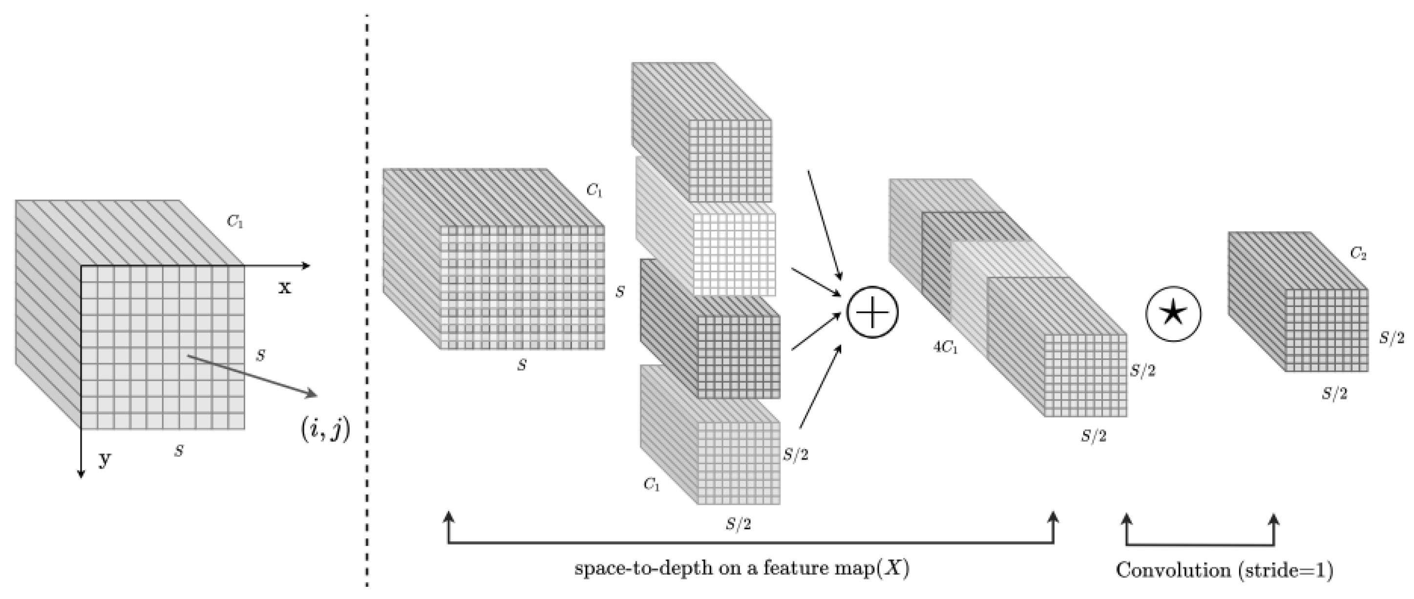
Figure 2.
Network structure of the CSRAM.
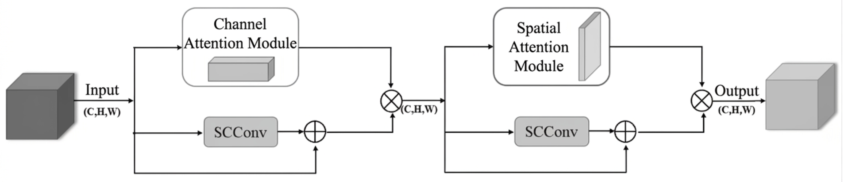
Figure 3.
Network structure of the CAM.
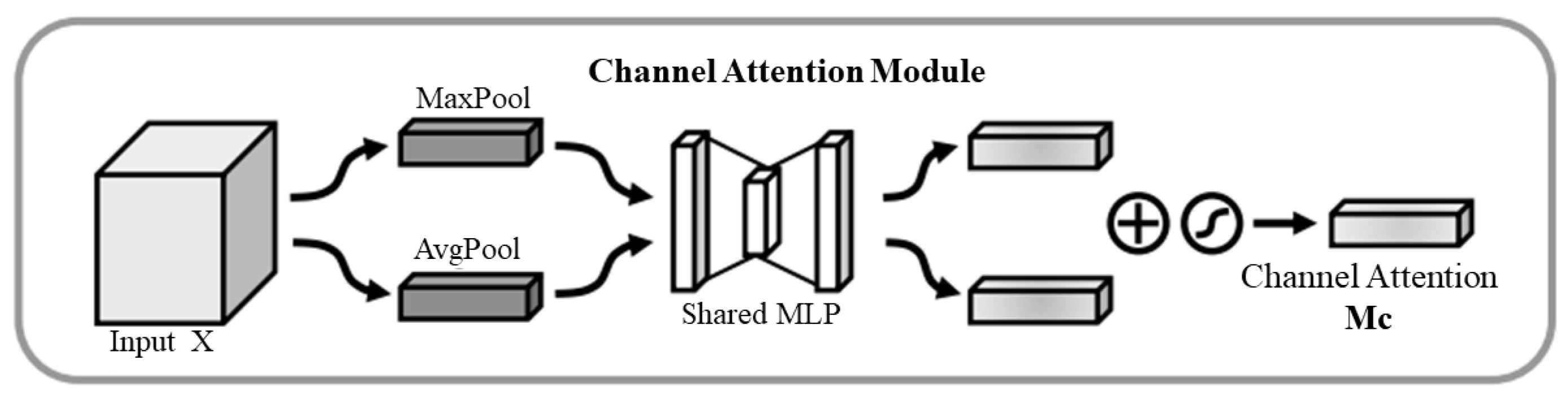
Figure 4.
Network structure of the SAM.
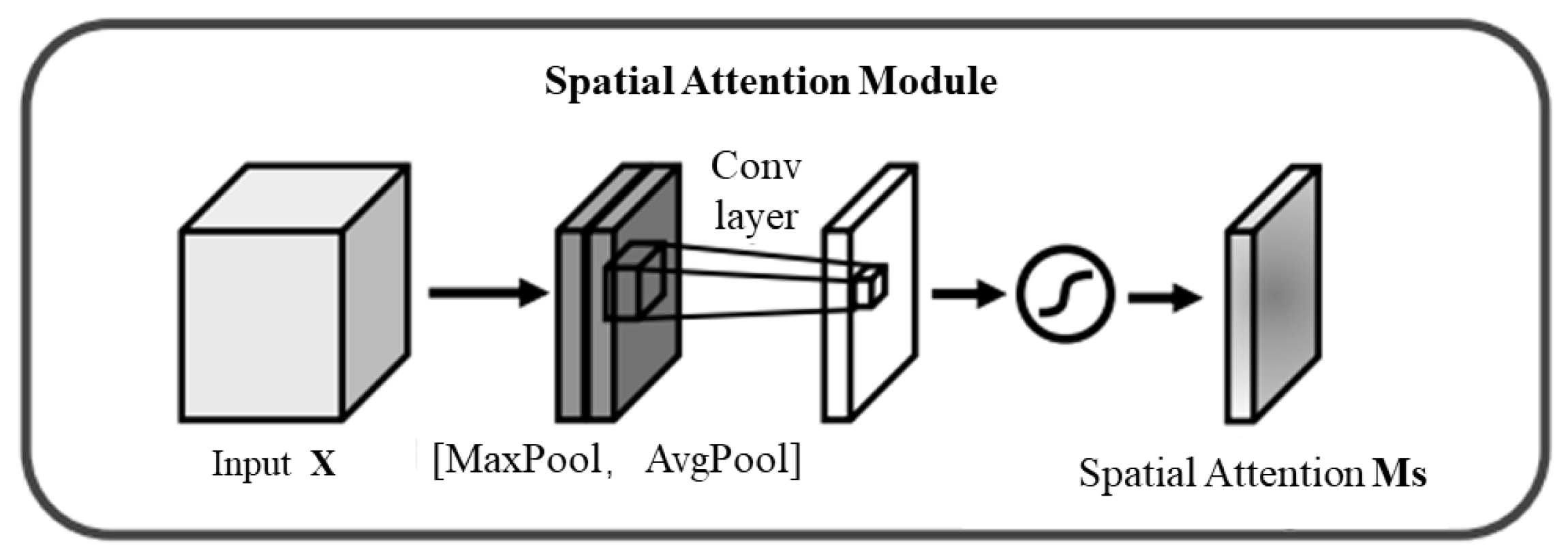
Figure 5.
Network structure of SCConv.
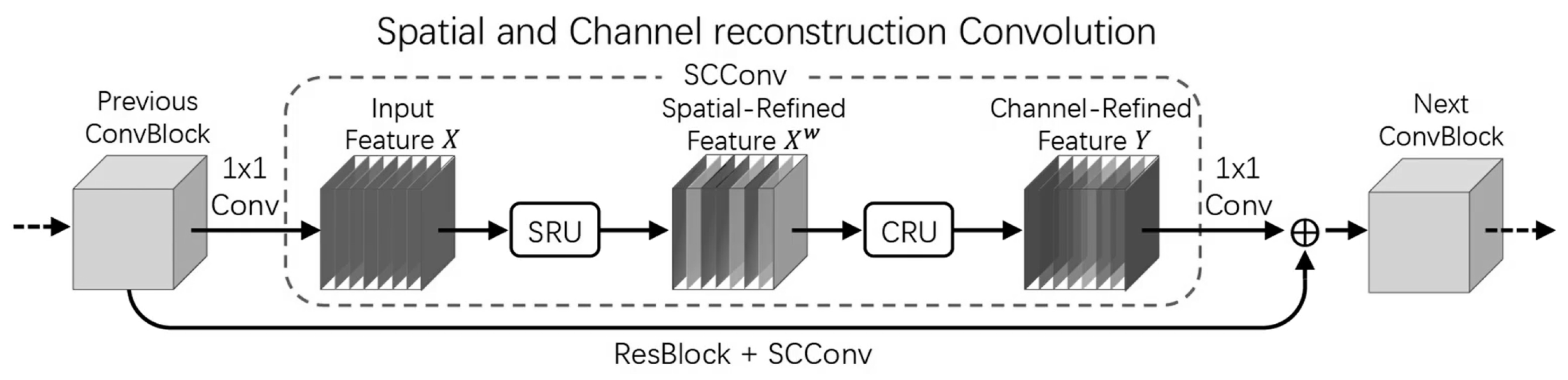
Figure 6.
Network structure of the SRU.
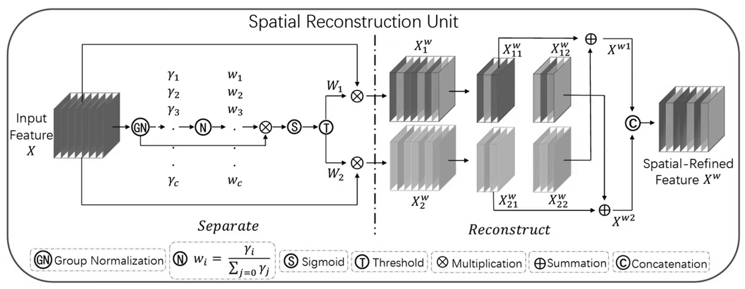
Figure 7.
Network structure of the CRU.
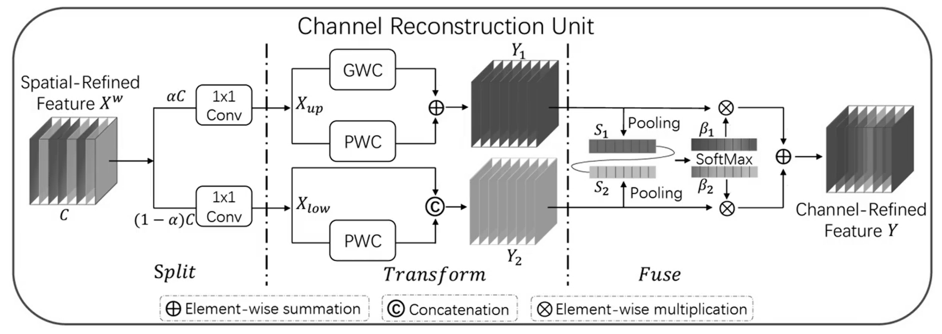
Figure 8.
Comparison of the gain coefficient r for different values of when is constant.
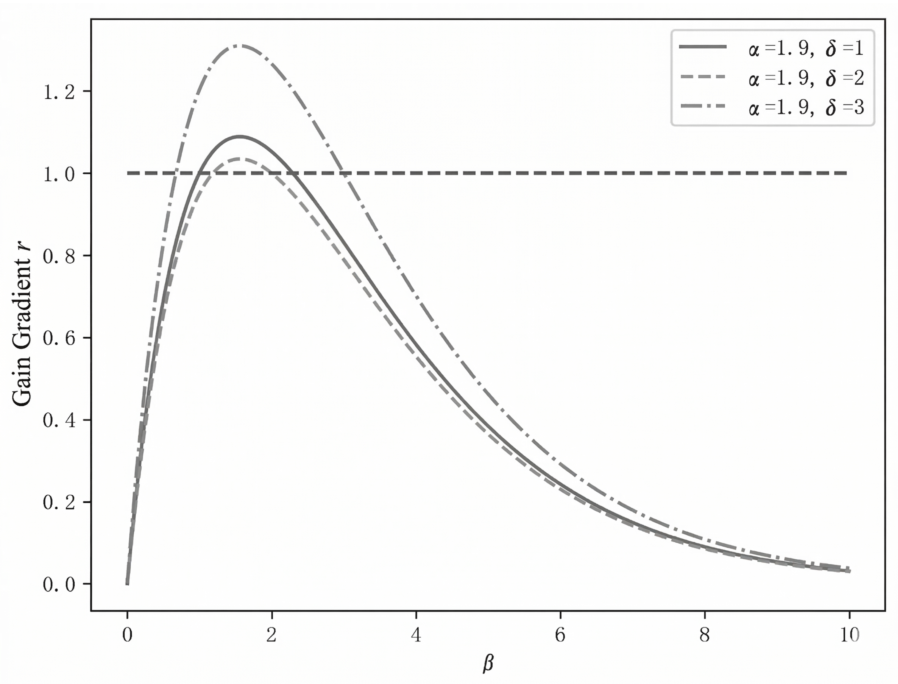
Figure 9.
Comparison results of feature heatmaps.
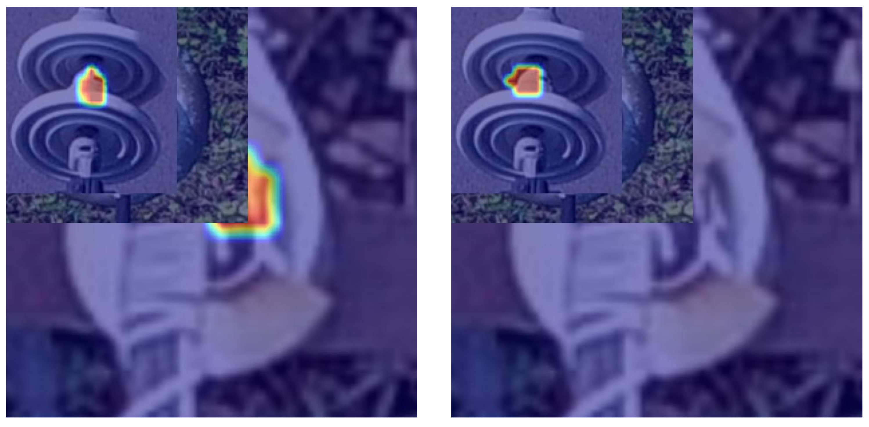
Figure 10.
Model comparison under complex working conditions: (a) Detection results using YOLOv8 baseline; (b) Detection results using our proposed improved model.
Figure 10.
Model comparison under complex working conditions: (a) Detection results using YOLOv8 baseline; (b) Detection results using our proposed improved model.
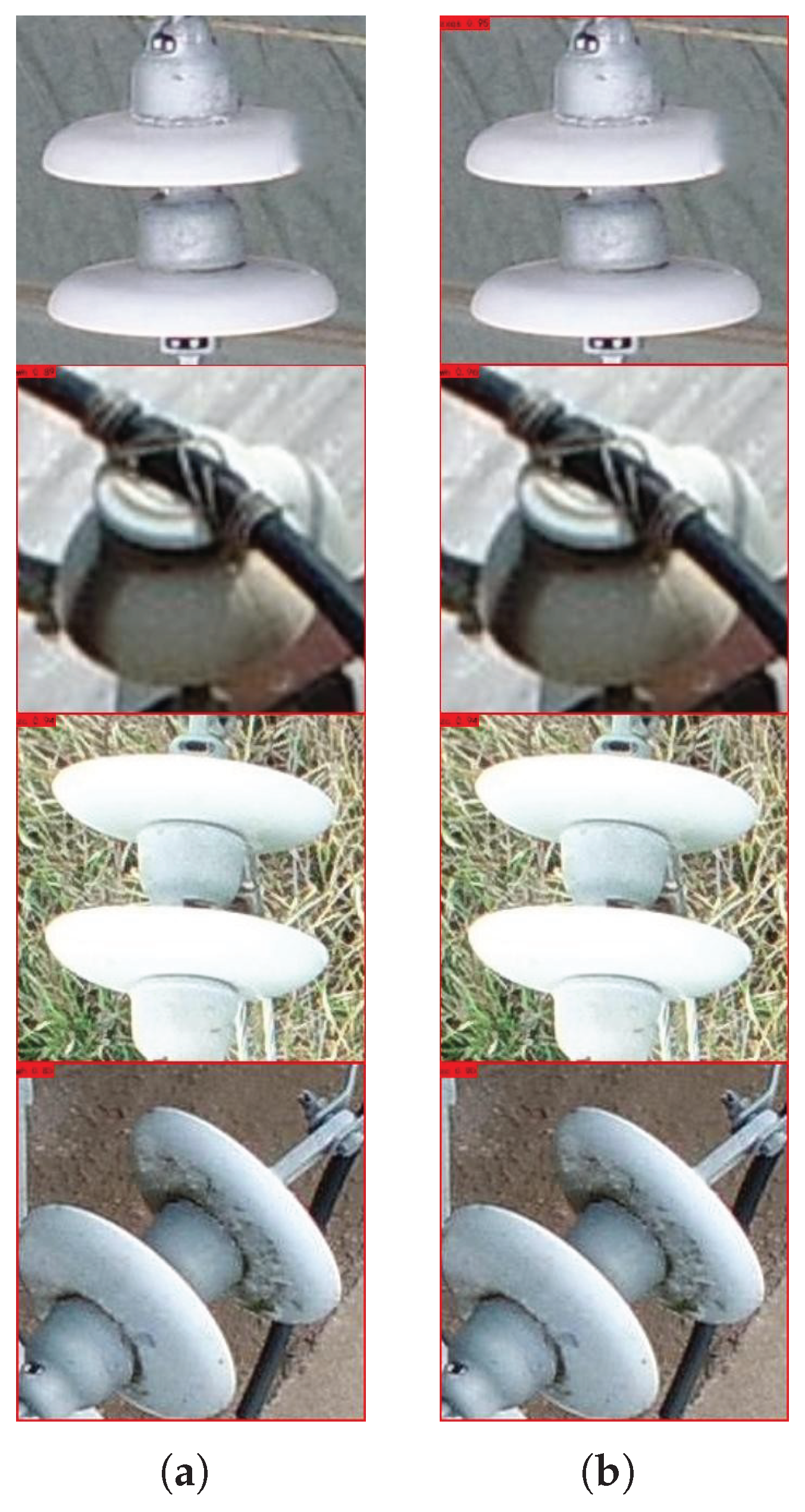

Table 1.
Software and hardware environment configurations.
| Configuration Item | Specification |
|---|---|
| Operating System | Linux-64 |
| GPU | NVIDIA RTX 4090D |
| Deep Learning Framework | PyTorch 2.4 |
| Computing Platform | CUDA 11.8 |
| Programming Language | Python |
Table 2.
Category and distribution statistics of the dataset.
| Category Label | Defect Type | Number of Images |
|---|---|---|
| zc | normal | 25009 |
| ps | broken | 1808 |
| wh | polluted | 42457 |
| zxqs | missing | 24186 |
| zxst | loose | 8301 |
| In total | - | 101760 |
Table 3.
Comparative experimental results of different object detection algorithms.
| Algorithm Model | P (%) | R (%) | mAP@0.5 (%) |
|---|---|---|---|
| YOLOv5 | 92.26 | 85.52 | 85.26 |
| YOLOv7 | 93.42 | 86.67 | 85.89 |
| YOLOv8 | 93.19 | 87.06 | 87.35 |
| RT-DETR | 94.13 | 91.27 | 90.82 |
| Ours | 94.44 | 91.01 | 91.75 |
Table 4.
Results of the ablation study for the improved modules.
| Strategy | (%) | mAP@0.5 | ||||
|---|---|---|---|---|---|---|
| Baseline | 85.91 | 71.66 | 94.70 | 96.90 | 87.59 | 87.35 |
| +SPD&SCC | 88.33 | 79.43 | 95.35 | 96.97 | 90.68 | 90.15 |
| +CSRAM | 89.79 | 80.87 | 95.87 | 97.02 | 92.51 | 91.21 |
| +Focal-wiou | 89.84 | 82.53 | 96.61 | 97.02 | 92.74 | 91.75 |
Disclaimer/Publisher’s Note: The statements, opinions and data contained in all publications are solely those of the individual author(s) and contributor(s) and not of MDPI and/or the editor(s). MDPI and/or the editor(s) disclaim responsibility for any injury to people or property resulting from any ideas, methods, instructions or products referred to in the content. |
© 2026 by the authors. Licensee MDPI, Basel, Switzerland. This article is an open access article distributed under the terms and conditions of the Creative Commons Attribution (CC BY) license (http://creativecommons.org/licenses/by/4.0/).
Copyright: This open access article is published under a Creative Commons CC BY 4.0 license, which permit the free download, distribution, and reuse, provided that the author and preprint are cited in any reuse.


