

Submitted:
15 March 2026
Posted:
17 March 2026
You are already at the latest version
Abstract
The paper proposes a model to predict users’ personal interests from their gaze. Current image processing technologies enable us to identify each user’s gaze and pupil diameter. However, they cannot identify user interests. The model uses deep learning technologies. It consists of mechanisms to handle the two kinds of gaze: one specific to individuals and the other common to many people. Its training method utilizes the human property that user interests in objects in vision affect their gaze. Since it is known that pupil diameters increase when users view what they are interested in, we can train the model to predict users’ personal interests using the pupil diameters as labels. Especially, the paper not only proposes a model structure to predict personal interests but also examines the process of the modification of parameters of the model to reveal requisites to predict personal interests from gaze. The method enables us to provide personalized information to each user, such as recommendations in VoD services, advertisements during e-shopping, plate annotations in restaurant menus, and so on.
Keywords:
gaze
; interest
; saliency map
; deep learning
; transformer
1. Introduction
Human interests vary from person to person. If we could predict what a person is interested in, there are a variety of potential applications, such as displaying advertisements during e-shopping for individual customers or presenting annotations for cuisines on restaurant menus based on personal preferences. The applications include targeted advertising, which attracts interest in appropriate products based on the user’s interests. It is based on the idea that the users’ interests are expressed in the content they search for and watch. Data obtained from the users brings the product recommendations [1,2,3]. These approaches have been actively researched in recommendation systems.
The collaborative filtering has achieved the greatest results in this field. The method assumes that user preferences are consistent across many users. It predicts the interests of a specific user based on the similarity with many users. Leveraging the interests shared by many users, collaborative filtering can recommend optimal products and advertisements. It enriches their lives.
However, collaborative filtering only works well when many users are interested in objects with known characteristics. It also assumes the user whose interests we want to predict shares common interests with many users. Collaborative filtering provides no benefit to grey sheep users, whose interests are only partially consistent with those of other users and have low correlation coefficients with almost all other users. The interests of users who have unique characteristics within a population are difficult to predict. Itis known as the grey sheep problem[4]. Because recommender systems must benefit all users, there have been many attempts to predict the interests of grey sheep users[5,6].
To identify the unique interests of a particular individual, it is meaningless to examine only characteristics common to a large number of users. It is necessary to predict items that will be of interest to each user based on their unique characteristics. To do this, we need indices whose value changes depending on the interests of each user. Such indices have only been calculated for specific media, such as [1,2,3]. If we could obtain an index that can identify users’ interests from their everyday activities, the power of recommendation systems could be extended to all fields.
A person’s gaze contains many meanings. Interest is one of them. It is known that a person’s gaze changes when what they are looking at is interesting to them. Because gaze directly expresses individual interests, it not only expresses the factors of persons’ interests but also reveals their characteristics. Furthermore, people would look at objects of interest. It does not place any extra burden on them. Gaze is a suitable indicator for predicting interests.
If we could predict an individual’s interests from their gaze, we could solve the Grey Sheep problem. However, to make the predictions, we need to use gaze information collected from individuals to train personal AI models. It requires a long time because the gaze information must be repeatedly presented to the model for training. A low-cost method is needed to build a model that can predict an individual’s interests from their gaze. It is necessary to clarify the structure of a prediction model that can be trained efficiently.
The study proposes a model structure for predicting individual interests from gaze. To achieve interest prediction at low cost, it first shows that individual interests affect the distribution of gaze. Second, to efficiently predict individual interests from gaze, the study proposes a model that combines a mechanism for predicting gazes common to many people with one for extracting individual interests. Both of the mechanisms are implemented using deep learning models. Finally, experiments reveal how parameters of the mechanisms are modified during training. They also demonstrate that parameters of a pre-trained mechanism for predicting gaze common to many people improve the training efficiency of extracting individual interests.
The proposed model enables us to know what interested individuals look at. Due to the model, the recommendations of products and advertisements benefit all users. Furthermore, the learning process elucidated in this study will lead to ideas for making individual interest predictions more efficient.
2. Gaze and Interests
2.1. Saliency Map
Human gaze moves continuously depending on the purpose. When there is no target to look at, the gaze moves randomly, which means random gaze movements do not indicate interest. On the other hand, when humans are interested, they will fix their gaze on the object of interest[7]. For a given task, gaze changes to complete it [8]. It comes from the dynamic switching of the attention focus. Experiments with paintings [9] have revealed that gaze movements of persons interested in paintings differ from those of people with no interest in the paintings, though they engage in the same task to view the paintings.
Saliency maps show which parts of an image are attracting attention. Let us consider periodically observing the points a person looks at for a specific image. A saliency map visualizes image areas where the person tends to put gaze by displaying a scatter of points indicating observed gaze on top of the image. Saliency maps are used in UI analysis[10] and clinical experiments using eye tracking[11], taking advantage of their properties. The study aims to predict image areas in which a person is interested. If gazes are focused on an object, there is a high possibility that the person is interested in the object. The study uses a saliency map to visualize differences in individual interests.
2.2. Pupil Diameter
The pupil diameters indicate whether a person is interested in something. It is known that the size of people’s pupils changes depending on their interests. When looking at something that interests them, their pupils expand. On the other hand, pupils get smaller when they see what does not interest them, their pupils constrict [12]. Observation of these changes in the pupils provides us with information about interests that simple staring fails to present.
Eye tracking is a technology for observing gaze. It uses a specialized sensor called an eye tracker to record where a person is looking. Many works using eye tracking have been actively studied in recent years. It is used in a wide range of fields, including psychology and HCI [13].
To generate a saliency map, eye tracking is used to observe where people are looking within an image[14,15]. Some eye trackers can observe not only the points people are looking at within an image, but also the pupil diameter. However, eye trackers are expensive because they measure gaze and pupil diameter simultaneously. Furthermore, note that targets of interest are identified from pupil diameter, not from the sliency map.
2.3. Predicting Gaze for Each User
Gaze changes depending on an individual’s interests. Even when viewing the same image under the same conditions, the objects that attract attention within the image would differ from person to person. An individual’s saliency map differs from a saliency map that aggregates the gazes of many people. A saliency map that predicts an individual’s gaze is referred to as a personalized saliency map (PSM), while a saliency map that aggregates the gazes of many people is referred to as a universal saliency map (USM).
To create a USM, we need an image and the distribution of gazes toward it. To predict the USM, a deep learning method trains a model using the difference of the model output from the distribution of gaze that many people actually put on the image. It optimizes the model to minimize the difference. Deep learning models with convolutional layers are often used to process images. Among them, many industrial examples adopt VGG models, which combine convolutional layers with ReLU functions [16].
To predict gaze for each individual, it is necessary to incorporate individual features into the gaze prediction model. To extract individual features, one work labels what each individual is looking at [17], while another provides a user embedding layer using PSM [18]. These predict gaze for each individual by directly incorporating individual features as numerical data.
Another work uses BART for user encoding[19]. It utilizes the ability to calculate relationships between data, a property of the attention mechanism. PSM prediction requires calculating the relationship between each individual’s interest and features within the image. The encoder layer of a Transformer model represents the relationship between them as keys and values. The decoder emphasizes the query based on the keys and values passed from the encoder layer[20]. The emphasis of features within the image with an individual’s interest vector enables us to build a model that predicts gaze for each individual. The method of using the attention mechanism to represent differences between individuals has also been applied to fields other than saliency map prediction[21,22].
2.4. Large-scale Data for Predicting Gaze
To predict individual gaze, a predictive model must be able to identify areas in an image where people are likely to gaze. Interesting factors must have sufficient characteristics to attract attention within the image. If there is no object in the image that attracts attention, gaze will likely be dispersed over a wide area. To reflect interest in a human saliency map, we need a mechanism that can predict factors that attract general attention.
Large-scale saliency map data is essential for building a gaze prediction model using deep learning. However, the amount of data required for deep learning is enormous. It is impractical to recruit subjects and create a saliency map dataset from scratch. It is a common way to use a saliency map dataset created in previous works to build a model for predicting the gaze of a large number of people.
One well-known dataset is the SALICON dataset. Participants use a mouse to indicate the object they are looking at in an image displayed on a personal computer. The data is collected on a large scale via a server, resulting in the SALICON dataset [23]. The gaze distribution in the dataset has been proven to be as accurate as a saliency map created using gaze data. The dataset adequately represents human gaze. Furthermore, the dataset contains 10,000 training images and 5,000 validation images, making it a sufficient amount for use as a deep learning dataset. Due to its large amount of data, it can be used to build a saliency map prediction model [24]. A gaze prediction model using the dataset guarantees the ability to predict general human gaze.
3. Gaze Model Reflecting Interest of Each User
3.1. Research Questions
The paper addresses the following research questions.
- Do interests affect persons’ gaze?
- Can we build a model that predicts the interests of persons with their gaze?
- What kinds of process does the model learn to predict interests with gaze?
Though the first would be right intuitively, we should confirm it through an experiment. The experiment would reveal the validity of the model configuration we assume in the second question. Once we have built the model, we can investigate the learning process of the model.
Interests vary with individuals. The model has to be trained for each user, which means it costs much to provide personal service. The investigation of the learning process would provide a way to solve the cost problem.
To address the questions, the paper handles two kinds of models to predict gaze for a specific image. One uses gaze data collected from a large number of people to predict a universal saliency map (USM), which indicates image parts where many people’s gazes are likely to be focused. The other predicts a personal saliency map (PSM), which indicates the image parts where an individual’s gaze is likely to be focused.
3.2. Model for Predicting USM
A model with complex mechanisms might make it unclear which configuration is effective for gaze prediction. The study builds a simple model.
Figure 1 shows the general gaze prediction model proposed in the study. The model is based on SalGAN, a well-known saliency map prediction model [25]. Since it follows the GAN mechanism, it consists of a generator and a discriminator. When predicting gaze, the study does not use a discriminator. It uses only the generator of a saliency map. The generator uses a VGG16 as its encoder. Its output is fed to the decoder to generate a USM. The model configuration is shown in Table 1 for the encoder and Table 2 for the decoder.
SalGAN uses a sigmoid function as the activation function for the final layer to use BCE (Binary Cross Entropy) as the loss function. However, the study uses a ReLU function. It results in a non-negative output. It allows us to use mean squared error as the loss function, which makes the accuracy of the generated saliency map easier to interpret intuitively.
In the study, to make the calculation light, the input image is compressed to 1/4 of its size. SalGAN can achieve sufficient accuracy even with input images compressed to 1/4. There is no impact on prediction results.
3.3. Collection of Saliency Maps from Individuals
To predict the interests of each individual, it is desirable that when persons view a specific image, the location where their gaze is focused differs depending on their interests. An example is shown in Figure 2. Suppose an image in which a rural landscape occupies the right half, while a motorcycle occupies the left half. Person A, who likes landscape paintings, primarily fixates on the right half. On the other hand, person B’s gaze will likely be focused on the motorcycle on the left half. For gazes to differ from person to person, the image should present various objects.
Based on the assumption that human gaze is drawn to areas within an image that contain meaning or context, the SALICON dataset is composed of images selected from the MS COCO dataset [26]. Each image in the dataset contains a variety of interesting objects.
Predicting a saliency map requires human gaze information collected for each image. Following the method used to create the SALICON dataset, gaze data collection using an eye tracker requires alternating between displaying an image for a certain period of time to have a person observe it and taking a break for a certain period of time. If the user is required to change the image, the operation increases the cognitive load on the person to introduce noise into the gaze information [27].
The study prepares a tool to collect gaze information. The data items collected per unit time by the gaze collection tool are shown in Table 3. Once launched, it will display an image that covers the entire screen. It allows the entire PC screen to be used for gaze collection, reducing noise during collection. After launching, the tool automatically switches between image presentation and rest phases. The image changes when switching from rest to image presentation.
3.4. Generating Saliency Maps for Individuals
The tool periodically collects the coordinates of the points on the image that the person is looking at. For each coordinate in the image, it calculates the number of times the gaze is fixed on the point within a certain period. The number indicates where the user is looking and for how long. The saliency map is created by applying a Gaussian filter to the number and representing it as a heat map between 0 and 1.
When gazes are concentrated around a specific image coordinate, the peak of the heat map will be higher than other image coordinates, emphasizing that gazes are focused on that object. Conversely, in areas where gazes are not concentrated, there will be no peak on the heat map at all.
Generating such a saliency map, we can express where and how much the person is looking as the probability of gaze appearing for each image coordinate, rather than as a simple set of gaze coordinates.
3.5. User Characteristic Vector
The study uses pupil diameter as an indicator of interest. However, just like changes in gaze, pupil diameter also changes from moment to moment. A simple comparison of pupil diameter between the previous and current times is insufficient to determine whether pupil diameter has changed due to interest. Furthermore, pupil diameter differs from person to person due to physical characteristics. Suppose we determine that interest exists when the change in pupil diameter exceeds a certain threshold. However, if a uniform threshold is applied to multiple persons, the influence of their unique pupil diameter size will make it impossible to accurately determine whether each of them is interested.
Suppose we record the change in pupil diameter over t seconds while a user is viewing an image. If a user views M images, we can observe the change in pupil diameter for each subject over seconds. If pupil diameter follows a Gaussian distribution, the histogram of pupil diameter over seconds should be bell-shaped, centered on the mean value, for each subject. If no changes in interest occur, pupil diameter will fluctuate around the mean value. On the other hand, if the pupil expands or contracts due to interest while viewing a particular image, the probability of large or small pupil diameter values increases. Therefore, the study calculates the Mahalanobis distance of the acquired pupil diameter for each user to perform an anomaly test. The significance level used in the test determines a threshold for pupil diameters that are larger or smaller than normal. Based on the threshold, we can extract images for which the pupil diameter enlarges for each subject.
For the experimental data set D, let be the pupil diameter at time t when person observes image . Using the function , is defined as follows:
The threshold value obtained by the abnormality test is A, which is set to 1 if the pupil diameter is enlarged and 0 otherwise. In this case, whether person is interested in image is defined using function as follows:
If we calculate it for all images to consider the tensor compiled for each subject, we get:
where . Tensor can be expressed as a matrix that satisfies
3.6. Building Model for Predicting PSM
The study incorporates a mechanism to account for individual characteristics within a general gaze prediction model described in Section 3.2. The structure separates the roles of each mechanism. It enables us to narrow down the mechanisms to be focused on in gaze analysis. The study refers to the mechanism that represents individual characteristics in a vector as the user encoding mechanism.
User Characteristics is a vector that reflects the unique features of each individual. The vector is essential to a model that predicts individuals’ gaze. As the user characteristics, the study adopts described in Section 3.5. Note that , which reflects the interests of person , is an M-dimensional vector.
Let us consider again the general gaze prediction model explained in Section 3.2. The encoder of the model extracts the characteristics from the input image using convolutional layers, while the decoder converts them into a saliency map. The encoder output is a tensor in which semantic compression has been completed for each pixel.
Let be the output from the encoder, B be the batch size, C be the number of channels, and W and H be the two side lengths of the output image. = If we see the tensor per batch size, If we regard it as a one-dimensional vector, If we consider it as a two-dimensional matrix, , we can think of it as a set of WD pixels with C-dimensional elements. The C-dimensional vector of each pixel is the result of the compression of the information surrounding the pixel. If the dot product of the C-dimensional vector and a vector representing a person’s interests is large, it indicates that the person is interested in the pixel. The dot product enables us to predict each individual’s gaze. Incorporating a Transformer into a model to predict USM, the study proposes a model to predict PSMs, as shown in Figure 3.
Using the attention mechanism of the transformer model, the model converts a pair of image features and user features into personal interests. First, consider the transformer’s encoder. A transformer requests that the number of channels in the input tensor of the decoder should match the number of channels in the output tensor of the encoder. In Figure 3, the output of the encoder of the model that predicts USM is connected to the input of the transformer decoder. The number of their channels is . Therefore, for the transformer decoder to work even when the output of the transformer encoder is incorporated, the number of output channels in the transformer encoder must be consistent with . However, the vector representing user characteristics is M-dimensional, which is different from the C-dimensionality of the number of channels in . Therefore, the model uses a linear layer for a dimension transformation.
Let be the input to the Transformer Encoder, and be the matrix that performs the linear transformation.
The output dimension of the encoder can have the same number of channels as , which enables the inner product with to be calculated. Through these processes, the user characteristics are fed to the transformer encoder. The self-attention mechanism extracts the user characteristics. The transformer encoder provides them for the transformer decoder as and .
Let the output from the transformer encoder be , and the input to the first-layer Transformer Decoder be . The attention for can be expressed as follows:
They hold regardless of the number of layers or heads in the transformer.
The saliency map pixels whose relationship with user characteristics has been emphasized by the transformer decoders is expected to fully encompass the interests of individual users. Finally, they are fed to the decoder to generate a saliency map. The saliency map whould reflect the user’s interests.
4. Evaluation with Experiment
4.1. Experiments
To collect gaze distribution, experiments use an eye tracker, Tobii Pro Nano, connected to a laptop PC with a screen size of pixels. The PC collects gaze distribution with a proprietary software tool through the eye tracker. Calibrating the eye tracker for each subject, the collection tool acquires gaze coordinates on the screen. The calibration allows more accurate acquisition of gaze distribution, eliminating physical differences between subjects.
The study involved 15 subjects, consisting of 12 men and 3 women, aged 21 to 25, with no color blindness and corrected vision. The subjects are asked to fill out a questionnaire about their hobbies. Though some subjects share common hobbies, no two subjects give the same answer. The experiments take place in a space with constant indoor lighting. The subjects sitting at a desk are instructed to view 1,000 images using the collection tool with periodic calibration.
The experiment uses 1,000 images from the SALICON dataset. All subjects view all of these images, because different images presented to each subject would prevent us from determining whether changes in gaze are caused by individual interest or by the inherent characteristics of the image. Each subject participates in an experiment comprising 20 sets of 50 images each. Subjects take regular breaks between sets to maintain their concentration. Each experiment is conducted over one or two days, with a duration of approximately three to four hours per subject.
A total of 12,550 gaze distribution samples are obtained in the experiment. Among them, the study analyzes 8,000 samples of six men and two women, which provide sufficient gaze distribution for all 1,000 images used in the experiment.
4.2. Gaze Difference among Subjects
Let us explore the answer to our first research question: "Do individual users’ interests influence their gaze on each image?" If subjects with different interests present almost the same gaze for given images, it is meaningless to construct a model to predict personal interest from gaze.
Let us explore the answer to the first research question: "Do individual users’ interests affect how they view each image?"
The data obtained through the eye tracker consists of gaze coordinates and pupil diameters. The study converts the gaze coordinates into a saliency map using a Gaussian filter, following the SALICON dataset [28].
Figure 4 shows, in monochrome, the distribution of all gaze coordinates for each of the eight subjects without considering the frequency of gaze occurrence at each coordinate. For all subjects, there are more gazes at the center of the image, while fewer at its edges. It is referred to as the central bias. It indicates that human gaze often converges on the center, while personal interests bring individual differences.
The differences between subjects are reflected in the cosine similarities for each subject, shown in Figure 5. The values on the vertical and horizontal axes represent each subject number. The cosine similarities for subjects 1 and 6 are particularly high, at 0.9878. We can also see that subject 4 is relatively similar to all other subjects, while subject 7 is low in similarity. However, the lowest value in Figure 5 is 0.9703, which means that the cosine similarities are high overall. The influence of the centeral bias is significant. We need to investigate whether there are any differences between subjects, excluding the center biases.
Figure 4, which does not reflect the frequency of gaze occurrence at each coordinate, does not tell us whether gazes are concentrated in a narrow area or spread over a wide area. Let us convert the gaze information into a PSM for each subject. Figure 6 shows the gaze distribution as a heat map. As gazes are accumulated at the same coordinate, each coordinate is represented in a color ranging from deep blue to yellow. Subjects 1, 4, 5, and 6 rarely direct their gaze to the edge of the image, i.e., their gazes are mostly fixed on the center. On the other hand, the gaze of subjects 0, 2, and 3 gathers slightly above the center. Finally, subject 7 directs the gaze widely throughout the entire image.
It could come from the fact that the objects photographers intend to capture are located at the center of many photographs used in the experiments [11]. The accuracy of the model trained using such datasets would get higher if its output is closer to the center. As evaluation metrics, the study should use sAUC (Shuffled AUC) and AUC-B (AUC-Borji), which can evaluate models while reducing the effects of the central bias [12]. Table 4 shows the accuracy of the PSM calculated from gaze data collected in the experiments, expressed as sAUC and AUC-B for each subject. In the table, even sAUC, which takes center bias into account, achieves a very high evaluation of 0.877. It indicates that the PSM collected in the experiments accurately represents the tendency for gaze to converge toward the center.
On the other hand, if the collected gaze distribution does not adequately represent differences between subjects, it is difficult to create a model that predicts individual gazes. The number of gaze coordinates the tool collects from each image is fixed to 300. As a result, the gaze distribution varies with subjects; the number of gazes around the center gets small, while the area where gazes gather will differ for each subject. It reduces central bias, which allows us to investigate individual gazes, including the influence of the unique characteristics of each image.
Let us compare PSMs between subjects. Figure 7 shows the average cosine similarity between subject PSMs. The differences can be regarded as the one in gaze patterns between subjects. Compared to Figure 5, the PSM similarity in Figure 7 is low. Subjects 1, 4, 5, and 6, who have high cosine similarity in Figure 5, also had relatively high cosine similarity in Figure 7. It indicates that subjects tend to fixate on the same object, that is, they exhibit similar gaze movements even when the influence of the central bias is suppressed. However, the maximum cosine similarity and the minimum are 0.593 and 0.372, respectively. The values are low as a whole.
The PSMs show high similarity due to the central bias, but they also present differences in gaze tendencies between individuals for each image. When humans are interested, they focus their gaze on the object of interest [6]. In answer to the first research question, we can say that differences in interest affect gaze. However, note that the differences among subjects are extremely small, with a maximum of 0.221. It would be undesirable to use PSMs as labels for training a gaze prediction model. We should prepare user feature vectors to be used for the labels.
4.3. Change of Pupil Diameters
The experiments record changes in pupil diameter over time for each image. Figure 8 shows a histogram of the pupil diameter for each subject after the standardization. If personal interests change the pupil diameter, the gaze distribution will differ from a Gaussian distribution, which represents randomness. It should result in gazes gathering in areas other than the average.
Figure 9 shows QQ plots of the samples in Figure 8. The red line represents the normal distribution. For most subjects, both ends of the distribution deviate significantly from normality. It indicates that a significant number of samples are distributed far from the average.
To demonstrate that the pupil diameter distribution deviates from normality, an anomaly test based on the chi-squared distribution is applied to extract both sides of the distribution. Two significance levels, 1% and 10%, are used to determine which is more effective in extracting pupil diameters that deviate from normality. It allows us to determine the degree of their deviation suitable to detect personal interests.
The QQ plot for subject 7 has an unusual shape compared to the other subjects. It has two centers. It could be due to the difference in the number of days spent on the experiment. While most subjects complete their experiments in one day, subjects 1 and 7 take two days. Figure 10 shows the pupil diameters of subjects 1 and 7, standardized by experiment day, in a histogram and QQ plot. They have the same shape as the distribution for the other subjects. Limited to subjects 1 and 7, the anomaly testing is applied to samples of each day to extract thresholds for their personal interests.
Figure 11 shows the pupil dilations for every subject at each significance level. The left and right graphs show the 1% significance level and 10% significance level, respectively. The vertical axis shows the identifiers of the 1,000 experimental images, while the horizontal axis shows the identifiers of each subject. In the graphs, if the pupil dilation is greater than the significance level for the image, it is depicted with the bright color, otherwise with the dark color. From the 1% significance level graph, we can see that pupil dilation depends on each subject. Greater pupil dilations are not uniformly distributed across all subjects. Some subjects barely present them. The bright areas of the 10% significance level cover those of the 1% significance level. However, even at the 10% significance level, there are images for which few subjects present pupil dilation.
The gaze collection tool used in the experiment measures pupil diameter approximately 300 times over 5 seconds. If pupil diameter changes randomly, regardless of the image, pupil dilation should be observed in almost all images. However, it is not the case in Figure 11. It suggests that there is some factor behind the change in pupil diameter. It has been shown that human pupil size varies with interest [29]. The pupil diameter is enlarged due to the subjects’ interest in the image’s characteristics. The paper regards the pupil dilation for each image as a user characteristic vector, which represents the interests of each subject.
Figure 12 shows the cosine similarity of interest for every pair of subjects at each significance level. The values on the vertical and horizontal axes represent each subject. Subjects 1 and 5 have high cosine similarity. It indicates that subjects 1 and 5 are often similar in interests, compared to other subjects. On the other hand, at a significance level of 1%, subject 4, whose gaze distribution is similar to those of the other subjects in Figure 7, has a low cosine similarity with the other subjects. While subject 4 is similar to the other subjects in gaze distribution, the images that interest him are different from those of the other subjects. A similar gaze distribution does not necessarily mean a similarity in interest.
As shown in Figure 11, when the significance level is set to 10%, subjects 3 and 5 judge most images as interesting. Their cosine similarity is 0.819, indicating a high similarity. On the other hand, when the significance level is set to 1%, there are few images judged as interesting by both subjects 3 and 5. Their cosine similarity is 0.132, indicating that they are no longer similar to each other. For all subjects, when the significance level is changed from 1% to 10%, the cosine similarity increases to a high value. The increase also occurs for subject 7, whose cosine similarity is low with all other subjects.
Indeed, user feature vectors at a significance level of 1% would strictly detect interest, but the strict detection of pupil diameters causes a risk of missing cases where the subject is interested. Actually, as shown in Figure 11, when the significance level is set to 1%, most subjects find no images interesting. It makes no sense. On the other hand, as Figure 11 shows, each subject presents individual interests in images when the significance level is set to 10%. It is plausible to adopt a 10% significance level to detect changes in pupil diameter that correspond to interest. Here, we should note that the detection of the significance level at 10% accounts for pupil diameter dilation due to image characteristics, which commonly affects many people.
4.4. A Model for Predicting General Gaze
A general gaze is a distribution of gazes that appear commonly among many people for a given image. Let us build a model to predict it. The study uses the SALICON dataset. Of the 10,000 training images, 1,000 have been used to identify user feature vectors and predict gazes. Using the remaining 9,000 images, a model is trained to predict general gazes. To reduce the model size and training costs, the input images are compressed to one-quarter their original size. As a result, the output images are also one-quarter the size.
The batch size during training is 32. The optimizer is Adam, with the learning rate 1.0-e5. To prevent overfitting, early stopping will take place if the loss on the validation data does not decrease for five consecutive iterations.
Table 5 shows the model’s performance, calculated on validation data from the SALICON dataset. The indices NSS and CC represent the saliency of gaze coordinates and the correlation between the predicted results and the ground truth map, respectively. Table 5 shows that the model’s performance is comparable to that of SalGAN. It demonstrates sufficient gaze prediction. The results suggest that the model’s parameters adequately represent general gaze characteristics. The study trains a model to predict individual gaze, setting the parameter values as its initial values.
4.5. A Model for Predicting Personal Gaze
The model for predicting individual gaze takes two inputs: the user feature vector and the image used to create the PSM. These inputs produce an output. The model is trained to reduce the output error from the PSM corresponding to the model’s input image. The study makes a set of two inputs and one output to train the model with a total of 8,000 sets of data. The model has the same encoder and decoder structure as the general gaze prediction model, which enables the parameters of a general gaze prediction model to be directly substituted for those of the trained model.
Of the total 8000 data sets, 6400 are used for training and 1600 for validation. As with general gaze prediction models, the input images and PSM are compressed to 1/4 their original size, and the output size is also set to 1/4. The user characteristic vector at a significance level of 10% is labeled as 1. The training data and validation data are divided so that the number of images labeled with 1 is uniform for each subject.
Based on CvT [28], a model that incorporates CNN into a Transformer, the study adopts AdamW as the optimizer, with a weight of 0.05, and a learning rate of 1.0-e6. The model trains each image eight times within one epoch. For this reason, when calculating the average for each batch size, certain image characteristics become more pronounced. Therefore, the batch size is set to 1. As with general gaze prediction models, early stopping is applied if the loss on the validation data does not decrease for five consecutive times.
The Transformer model used in the user encoding mechanism is divided into a Transformer Encoder and a Transformer Decoder. Each of these can have any number of layers. It is necessary to determine the optimal combination of the number of layers for the Transformer Encoder and Transformer Decoder. Furthermore, the number of heads can be changed to account for multi-head attenuation in the Transformer model. The study first fixes the number of heads to 32 and the user feature vector at a significance level of 10% to determine the optimal combination of layers for the Transformer Encoder and Transformer Decoder that minimizes the error of the validation data. If the parameters of the model predicting general gaze are used as initial values, the influence of the mechanism encoding user features gets weak, which makes it difficult to observe differences in the number of Transformer layers. The study does not use the parameters of the model predicting general gaze to examine the number of layers.
Table 6 shows the number of layers and the corresponding loss function output. MSE is used as the loss function. Since the batch size is 1, the values in the table are simply the average MSE for all 1,600 validation data. Experimental results show that the error is minimized when the Transformer Encoder and Decoder have four and nine layers, respectively. The self-attention translates the user feature vector, which is input to the Transformer Encoder. The optimal number of layers differs between the Transformer Encoder and the Transformer Decoder because the more layers there are, the less the user feature vector represents the characteristics of the image features. It is necessary to limit the number of layers in the Transformer Encoder so that the user feature vector can represent the unique relationship of each individual with each pixel in the image.
Next, let us examine the effect of the number of multi-heads. Setting the Transformer Encoder to four layers and the Transformer Decoder to nine layers, the examination changes the number of heads to find the number that minimizes the error. The examination incorporates the parameters of a general gaze model into the learning process. It keeps the number of layers in the user encoding mechanism, as well as the encoder and decoder sections, in their optimal states, allowing us to investigate the effect of pure multi-heads.
Table 7 shows the results of the examination when the significance level for setting user feature vectors is 1% and 10%, and the number of heads for the Transformer Encoder and Transformer Decoder is changed to 32, 64, 128, and 256. The table shows that the error is minimized when the significance level for creating user feature vectors is 10%, and the number of heads is 256. Furthermore, as the number of heads increases, a gradual decrease in error can be observed in most cases. Let us add a case where the significance level is 10%, and the number of heads is 512. The table shows that the error increases when the number of heads is 512. It might occur because the number of heads assigned to each CNN filter in the Encoder section decreases as the number of heads increases. When the number of heads is 512, one head is assigned to each filter in the final layer, which means that the Transformer’s Query, Key, and Value become one-dimensional, making it difficult to represent individual characteristics properly.
The above shows that each element has a unique meaning in the user feature vector at a significance level of 10%. By paying attention to each element, the vector can clarify differences in individual subjects. However, it is interesting to note that the error is smaller at a significance level of 10% than at a significance level of 1%, and that the error increases when we pay attention to too few elements. At a significance level of 10%, attention includes factors common to more subjects. Factors are represented by multiple elements of the vector. If the elements are separated one by one, the vectors cannot fully represent the differences between subjects. It is consistent with the idea that we have better to consider image characteristics common to many people to detect pupil diameter dilation, as explained in Section 4.3. User feature vectors should be designed with the influence of general image characteristics in mind.
Based on the above examination, the optimal model for predicting an individual’s gaze should use a user characteristic vector obtained at a significance level of 10%, taking into account the influence of general image characteristics. The model should have four layers of Transformer Encoder, nine layers of Transformer Decoder, and 256 heads.
Table 8 shows the performance of the model for predicting personal gaze at optimal parameter settings. Subject 7 has the lowest sAUC of 0.7145, while the average is 0.7758. The model can express the gaze of each subject. Among the subjects, the model has the highest prediction for subjects 1 and 6.
Figure 13 shows an example output. The top row shows the input image, the middle row shows the model prediction results, and the bottom row shows the saliency map obtained from the subject’s gaze. Below the saliency map are the loss values. It can be seen that the model output tracks the differences in the position and spread of the saliency map for each subject.
5. Relationship between General Gaze and Individual Gaze
Section 4 has revealed that predicting individual gaze distribution requires an optimal model structure and a user characteristic vector that includes not only individual characteristics but also factors common to many subjects. However, it has not investigated the reasons why they are useful for predicting individual gaze distribution. This section uses the results of Section 4 to discuss the elements necessary for predicting individual gaze distribution.
A single USM is attained, aggregating the gaze data of multiple subjects for the SALICON dataset. The parameters of the model trained to predict the USM sufficiently reflect information about general gaze. Through analyzing how these parameters affect the prediction of individual gaze, we can clarify how differences between general and individual gaze arise.
The previous section examines the performance of the training model, both with and without the parameters for general gaze prediction as initial values. It turns out that training incorporating a general gaze prediction mechanism is more successful in making predictions that reflect individual differences between subjects. However, to understand the effect of the parameters, we needed to visualize the internal state of the model.
5.1. Model to Verify Hypothesis
To predict USM, which is a general gaze, the study trains a mechanism comprising an encoder that maps an input image to a code and a decoder that reconstructs the code into an image. As shown in Figure 14, the study adds a user-encoding mechanism to the model to incorporate each user’s characteristics. The configuration is adopted because the study assumes that an individual’s gaze is a variation of a general gaze.
The Linear layer of the user encoding mechanism embeds the user characteristics so that they can be fed to the Transformer layer. EmbUserCharacteristics is the user characteristic vector mapped by the Linear layer. EncUserCharacteristics is the user characteristic vector after being transformed by the TransformerEncoder layer. Rather than training a model from scratch, its initial values are set to the trained parameters of a model that predicts USM. The paper discusses how the learning progresses, examining the output of each mechanism.
The Enc Output of the model is an image generated by the decoder from the encoder output, without passing it through the user encoding mechanism. By comparing the Enc Output with the inherent output, we can visualize the impact of the user encoding mechanism on gaze prediction. The paper compares them when the parameters of the model that predicts USM are used as the initial values during training, and when they are not. It investigates the impact on gaze prediction
5.2. Training Independent of USM Parameters
Figure 15 shows the learning curve for the model trained with parameters of the encoder and decoder initialized with random values. It is a training using the encoder and decoder independent of the USM. The horizontal axis represents the number of epochs, while the vertical axis represents the error. In this study, if the lowest error value for the validation data is not updated for five successive times, early stopping is used to stop training. In the experiment, the learning stopped at 53 epochs. The figure indicates that the error for both the training and the validation data drops significantly around 20 epochs.
Figure 16 is a visualization at 20 epochs, while Figure 17 is one at the end of the learning. In both figures, from top to bottom, the input image, predicted gaze, visualized Enc Output, and actual gaze collected from the subjects are arranged for eight subjects. The visualization in Figure 17 indicates that each subject’s gaze is predicted to some extent, because the output follows the actual gaze in each subject.
The pixels in EncOutput are almost 0 in Figure 16. The result indicates that the encoder has rarely learned at the 20th epoch point. However, the output for each subject does not provide 0, but a monotonous rectangle. It is different for each subject. In terms of deviation from the center, the output is coincident with the actual gaze indicated by the “True” label. In Figure 17, we can see that Enc Output provides high values widely across the entire image. The figure also shows that the output is more consistent with the actual gaze distribution of each subject than that of Figure 16. Since the gaze distribution of each subject is the subject’s common gaze over many images, it presents a gaze tendency unique to the subject. It means the user encoding mechanism learns each subject’s unique gaze tendency earlier than the other parts. The results imply that the user encoding mechanism alone predicts an individual subject’s gaze using each subject’s unique gaze tendency in the early stage of the learning where the model is trained independently of USM parameters.
5.3. Training Based on USM Parameters
Figure 18 shows the learning curve of the model when the decoder and encoder parameters that predict USM are given as initial values. The learning ends after epoch 25. The learning finishes earlier than the training using parameters independent of USM.
Figure 19 is a visualization of the training results based on USM parameters. Compared to Figure 17, which shows the training results independent of USM parameters, EncOutput is significantly different.
Figure 20 is a visualization of a model that predicts USM. The model parameters are reused for predicting PSMs. The model proposed in the study predicts gaze for each individual by adding a user encoding mechanism. In Figure 19, the output has a shape made from the gaze distribution of the USM. It can be assumed that the model learns to predict individual gaze distribution, altering the given USM as a reference.
5.4. Predictability of PSM with Gaze
The second research question of the paper asks whether personal interests can be predicted by gaze.
Let us examine how much difference the USM parameters bring to vectors representing characteristics of each subject. Table 9 shows the cosign similarity of Emb User Characteristics with and without the USM parameters, while Table 10 shows that of Enc User Characteristics, respectively. Emb User Characteristics do not change significantly with USM parameters, but there is a large difference in Enc User Characteristics converted by the Transformer Encoder layer. The information required by each mechanism differs depending on whether USM parameters are used as the initial values. It might come from the foundation of the learning. Learning independent of USM parameters is founded on the commonality of each subject’s gaze across images, whereas learning based on USM parameters is founded on similarity to USM.
Figure 21 shows the cosine similarity between subjects for Enc User Characteristics. There is not much difference in the similarity. For example, subjects 3 and 5 are highly similar, while subjects 2 and 6 are low in similarity. The user characteristic vector used as input has 800 dimensions, while Enc User Characteristics has 512 dimensions, the same as the input dimensions of the Transformer Decoder layer. The Transformer Encoder extracts information from the inputs. The two vectors of EncUserCharacteristics based on/independent of USM parameters are coincident in subject similarity because the Transformer Encoder succeeds in extracting interest differences between subjects.
The results show that the model is trained to represent differences in user characteristic vectors, regardless of whether USM parameters are used. We can predict personal interests with gazes, which is the answer to the second research question.
5.5. Requisites for Predictability of PSM
Naturally, pupil diameter will expand not only when each individual has a unique interest, but also when there is an object that everyone is paying attention to. The user characteristic vector in the study represents pupil diameter expansion due to each subject’s interest, as well as pupil diameter expansion due to image characteristics that attract the attention of many people.
Within an image, individual gazes are drawn to objects matching the individual’s interest factors, starting from objects attracting many people. The output of the encoder, which predicts common gazes among many people, picks up objects that may be interesting to the subject. The study regards individual gazes as variations of gazes common to many people. Based on the person’s gaze tendencies, the variations arise according to characteristic objects in the image. It is explained by the change in the output of the model independent of USM parameters; it is first individual gaze tendencies, and then changes according to each image. Individual differences in gaze do not arise solely from interesting objects specific to individual interests within an image. It is reasonable to consider that they arise when objects attracting many people get the subject’s unique interests. As stated in Section 4.5, the user characteristic vector should include not only individual-specific characteristics but also the influence of general image characteristics.
Training with USM parameters as initial values corresponds to alternation of the initial position of learning. The state of learning is represented by a set of weights to be trained. The USM parameters affect the learning process because the learning proceeds through the error space along different paths depending on the initial position. If the initial position is located in a location far from the USM, the model takes a path in which it first attains the individual’s gaze tendency, next following the path to reach the USM. The fact that models reach similar results even in different paths indicates that the point of the smallest error is located in a certain area in the error space. The area passed during learning to attain the individual’s gaze tendency might partially overlap that passed during learning to attain the USM. The results suggest that the optimal point for PSM might be located in a hyperspace between an area for USM and one for an individual’s gaze tendency. When a model has mechanisms that represent the two areas, we can predict PSM.
Based on the above discussion, the model proposed in the study for individual gaze prediction requires the following four elements:
- mechanism that can predict general gaze,
- mechanism that can predict personal gaze,
- A training dataset containing common gaze patterns among many people, and
- A training dataset containing individual gaze characteristics.
It is the answer to the third research question. Note that a single dataset may contain both of the last two items.
6. Conclusion
The study proposes a method for predicting individual interests from their gaze. To predict gaze that reflects each individual’s interests, it builds a model for predicting PSMs. Experimental results have shown that, to express each individual’s gaze, it is necessary to combine two different mechanisms with different roles: a mechanism for predicting general gaze and one for expressing each individual’s gaze tendencies. The results also reveal that we should use two different characteristics: characteristics that represent general gaze and those that represent differences in gaze for each individual. The results of the study enable us to predict each individual’s PSM, which leads to objective identification of the interests of each individual.
The study examines only eight subjects. It has not been verified whether the model works for all individual characteristics. When adding a new person to the prediction target, the proposed method requires making a user characteristic vector. The vector is dependent on individual interests in the images used in the experiment. As a result, when adding a new subject, it is necessary to record gaze and pupil diameter. It poses the problem of high implementation costs per subject. To reduce the cost of applying the model, it is necessary to verify whether the model works consistently with vectors representing interest factors extracted using other methods with low implementation costs.
Author Contributions
Conceptualization, Aoba Izumi, Fumiko Harada, and Hiromitsu Shimakawa; formal analysis, investigation, Aoba Izumi, Fumiko Harada, and Hiromitsu Shimakawa; writing—original draft preparation, Aoba Izumi.; writing—review and editing, Hiromitsu Shimikawa.; visualization, Aoba Izumi; supervision, Fumiko Harada and Hiromitsu Shimakwa.
Funding
This research received no external funding
Informed Consent Statement
Informed consent was obtained from all subjects involved in the study.
Conflicts of Interest
The authors declare no conflicts of interest.
References
- Gomez-Uribe, C.A.; Hunt, N. The Netflix Recommender System: Algorithms, Business Value, and Innovation. ACM Trans. Manage. Inf. Syst. 2016, 6. [Google Scholar] [CrossRef]
- Mobasher, B.; Cooley, R.; Srivastava, J. Automatic personalization based on Web usage mining. Commun. ACM 2000, 43, 142–151. [Google Scholar] [CrossRef]
- Hong, L.; Davison, B.D. Empirical study of topic modeling in Twitter. In Proceedings of the Proceedings of the First Workshop on Social Media Analytics, New York, NY, USA, 2010; SOMA ’10, pp. 80–88. [Google Scholar] [CrossRef]
- Srivastava, A. Gray Sheep, Influential Users, User Modeling and Recommender System Adoption by Startups. In Proceedings of the Proceedings of the 10th ACM Conference on Recommender Systems, New York, NY, USA, 2016; RecSys ’16, pp. 443–446. [Google Scholar] [CrossRef]
- Gras, B.; Brun, A.; Boyer, A. Identifying Grey Sheep Users in Collaborative Filtering: A Distribution-Based Technique. In Proceedings of the Proceedings of the 2016 Conference on User Modeling Adaptation and Personalization, New York, NY, USA, 2016; UMAP ’16, pp. 17–26. [Google Scholar] [CrossRef]
- Huang, T.; Zhang, D.; Bi, L. Neural embedding collaborative filtering for recommender systems. Neural Computing and Applications 2020, 32, 17043–17057. [Google Scholar] [CrossRef]
- Hirayama, T.; Dodane, J.B.; Kawashima, H.; Matsuyama, T. Estimates of User Interest Using Timing Structures between Proactive Content-Display Updates and Eye Movements. IEICE Transactions 2010, 93-D, 1470–1478. [Google Scholar] [CrossRef]
- Tatler, B.; Wade, N.; Kwan, H.; Findlay, J.; Velichkovsky, B. Yarbus, Eye Movements, and Vision. i-Perception 2010, 1, 7–27. [Google Scholar] [CrossRef]
- Koide, N.; Kubo, T.; Nishida, S.; Shibata, T.; Ikeda, K. Art expertise reduces influence of visual salience on fixation in viewing abstract-paintings. PLoS One 2015, 10, e0117696. [Google Scholar] [CrossRef]
- Jiang, Y.; Leiva, L.A.; Rezazadegan Tavakoli, H.; R. B. Houssel, P.; Kylmälä, J.; Oulasvirta, A. UEyes: Understanding Visual Saliency across User Interface Types. In Proceedings of the Proceedings of the 2023 CHI Conference on Human Factors in Computing Systems, New York, NY, USA, 2023; CHI ’23. [Google Scholar] [CrossRef]
- Tseng, P.H.; Cameron, I.G.M.; Pari, G.; Reynolds, J.N.; Munoz, D.P.; Itti, L. High-throughput classification of clinical populations from natural viewing eye movements. Journal of Neurology 2013, 260, 275–284. [Google Scholar] [CrossRef] [PubMed]
- Groner, R.; Groner, M.T. Attention and eye movement control: An overview. European archives of psychiatry and neurological sciences 1989, 239, 9–16. [Google Scholar] [CrossRef]
- Plopski, A.; Hirzle, T.; Norouzi, N.; Qian, L.; Bruder, G.; Langlotz, T. The Eye in Extended Reality: A Survey on Gaze Interaction and Eye Tracking in Head-worn Extended Reality. ACM Comput. Surv. 2022, 55. [Google Scholar] [CrossRef]
- Wenclik, L.; Touya, G. EyeCatchingMaps, a Dataset to Assess Saliency Models on Maps. 2024. [Google Scholar] [CrossRef]
- Borji, A.; Itti, L. CAT2000: A Large Scale Fixation Dataset for Boosting Saliency Research. CoRR 2015. abs/1505.03581, [1505.03581]. [Google Scholar]
- Simonyan, K.; Zisserman, A. Very Deep Convolutional Networks for Large-Scale Image Recognition, 2015. arXiv arXiv:cs.
- Xu, Y.; Gao, S.; Wu, J.; Li, N.; Yu, J. Personalized Saliency and its Prediction. arXiv 2018, arXiv:cs. [Google Scholar] [CrossRef] [PubMed]
- Strohm, F.; Bâce, M.; Bulling, A. Learning User Embeddings from Human Gaze for Personalised Saliency Prediction. arXiv 2024, arXiv:cs. [Google Scholar] [CrossRef]
- Jiang, Y.; Guo, Z.; Tavakoli, H.R.; Leiva, L.A.; Oulasvirta, A. EyeFormer: Predicting Personalized Scanpaths with Transformer-Guided Reinforcement Learning. arXiv 2024, arXiv:cs. [Google Scholar]
- Vaswani, A.; Shazeer, N.; Parmar, N.; Uszkoreit, J.; Jones, L.; Gomez, A.N.; Kaiser, L.; Polosukhin, I. Attention Is All You Need, 2023. arXiv arXiv:cs.
- Tran, T.; You, D.; Lee, K. Quaternion-Based Self-Attentive Long Short-term User Preference Encoding for Recommendation. In Proceedings of the Proceedings of the 29th ACM International Conference on Information & Knowledge Management, New York, NY, USA, 2020; CIKM ’20, pp. 1455–1464. [Google Scholar] [CrossRef]
- Wu, L.; Li, S.; Hsieh, C.J.; Sharpnack, J. SSE-PT: Sequential Recommendation Via Personalized Transformer. In Proceedings of the Proceedings of the 14th ACM Conference on Recommender Systems, New York, NY, USA, 2020; RecSys ’20, pp. 328–337. [Google Scholar] [CrossRef]
- Jiang, M.; Huang, S.; Duan, J.; Zhao, Q. SALICON: Saliency in Context. In Proceedings of the 2015 IEEE Conference on Computer Vision and Pattern Recognition (CVPR), 2015; pp. 1072–1080. [Google Scholar] [CrossRef]
- Linardos, A.; Kümmerer, M.; Press, O.; Bethge, M. DeepGaze IIE: Calibrated prediction in and out-of-domain for state-of-the-art saliency modeling. arXiv 2021, arXiv:cs. [Google Scholar]
- Pan, J.; Ferrer, C.C.; McGuinness, K.; O’Connor, N.E.; Torres, J.; Sayrol, E.; i Nieto, X.G. SalGAN: Visual Saliency Prediction with Generative Adversarial Networks. arXiv 2018, arXiv:1701.01081. [Google Scholar] [CrossRef]
- Lin, T.Y.; Maire, M.; Belongie, S.; Bourdev, L.; Girshick, R.; Hays, J.; Perona, P.; Ramanan, D.; Zitnick, C.L.; Dollár, P. Microsoft COCO: Common Objects in Context, 2015. arXiv arXiv:cs.
- Alter, A.; Oppenheimer, D.; Epley, N.; Eyre, R. Overcoming Intuition: Metacognitive Difficulty Activates Analytic Reasoning. Journal of Experimental Psychology: General 2007, 136, 569–576. [Google Scholar] [CrossRef]
- Xu, J.; Jiang, M.; Wang, S.; Kankanhalli, M.S.; Zhao, Q. Predicting human gaze beyond pixels. J. Vis. 2014, 14. [Google Scholar] [CrossRef] [PubMed]
- E.H., H.; J.M., P. Pupil Size as Related to Interest Value of Visual Stimuli. Science 1960, 132, 349–350. [Google Scholar] [CrossRef] [PubMed]
Figure 1.
Model for Predicting USM

Figure 2.
Saliency Maps Dependent on Individuals
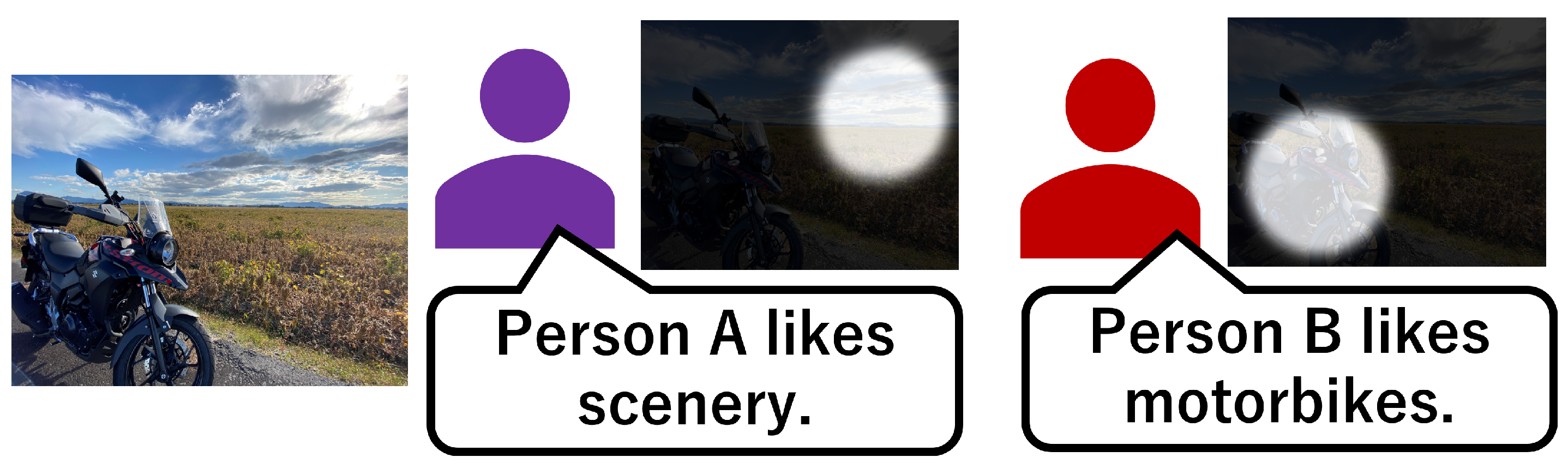
Figure 3.
Model for Predicting PSM
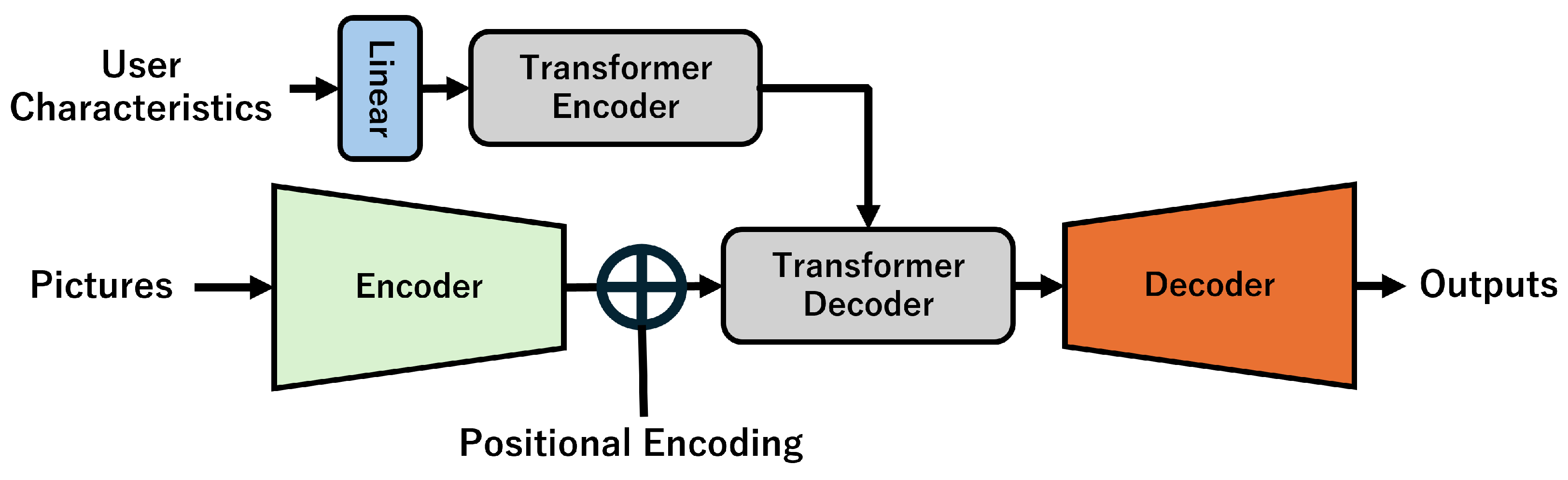
Figure 4.
Distribution of All Gaze Coordinates for Subjects
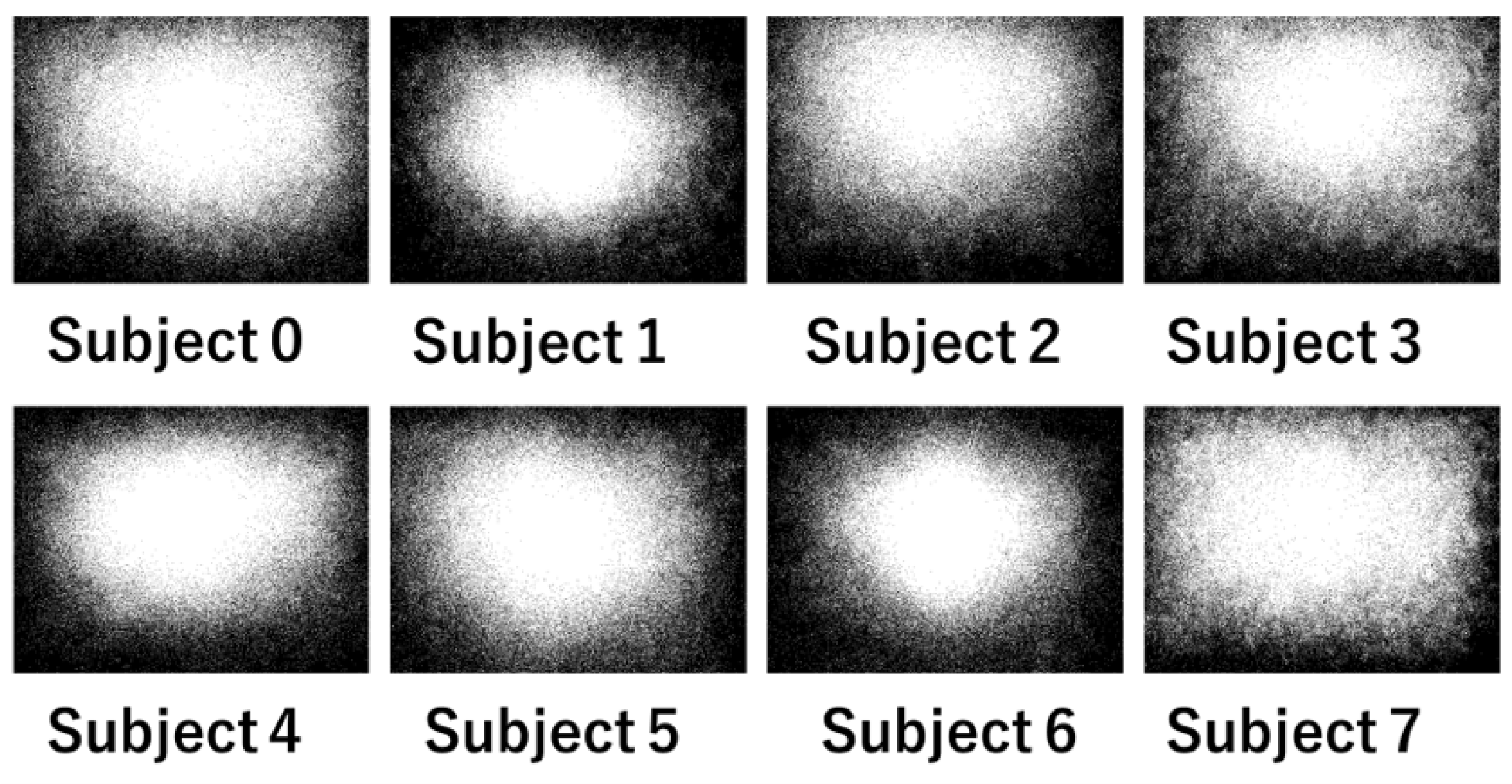
Figure 5.
Cosine Similarities between Subject Gaze Distribution without Normalization
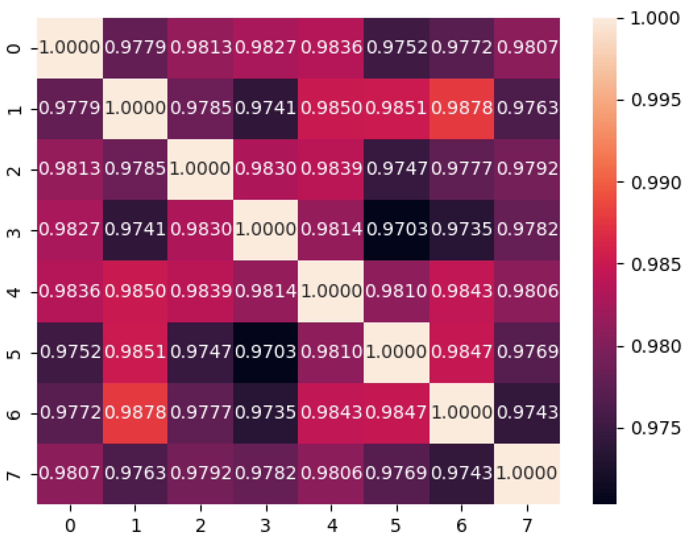
Figure 6.
Heat Map of Gaze Distribution without Normalization
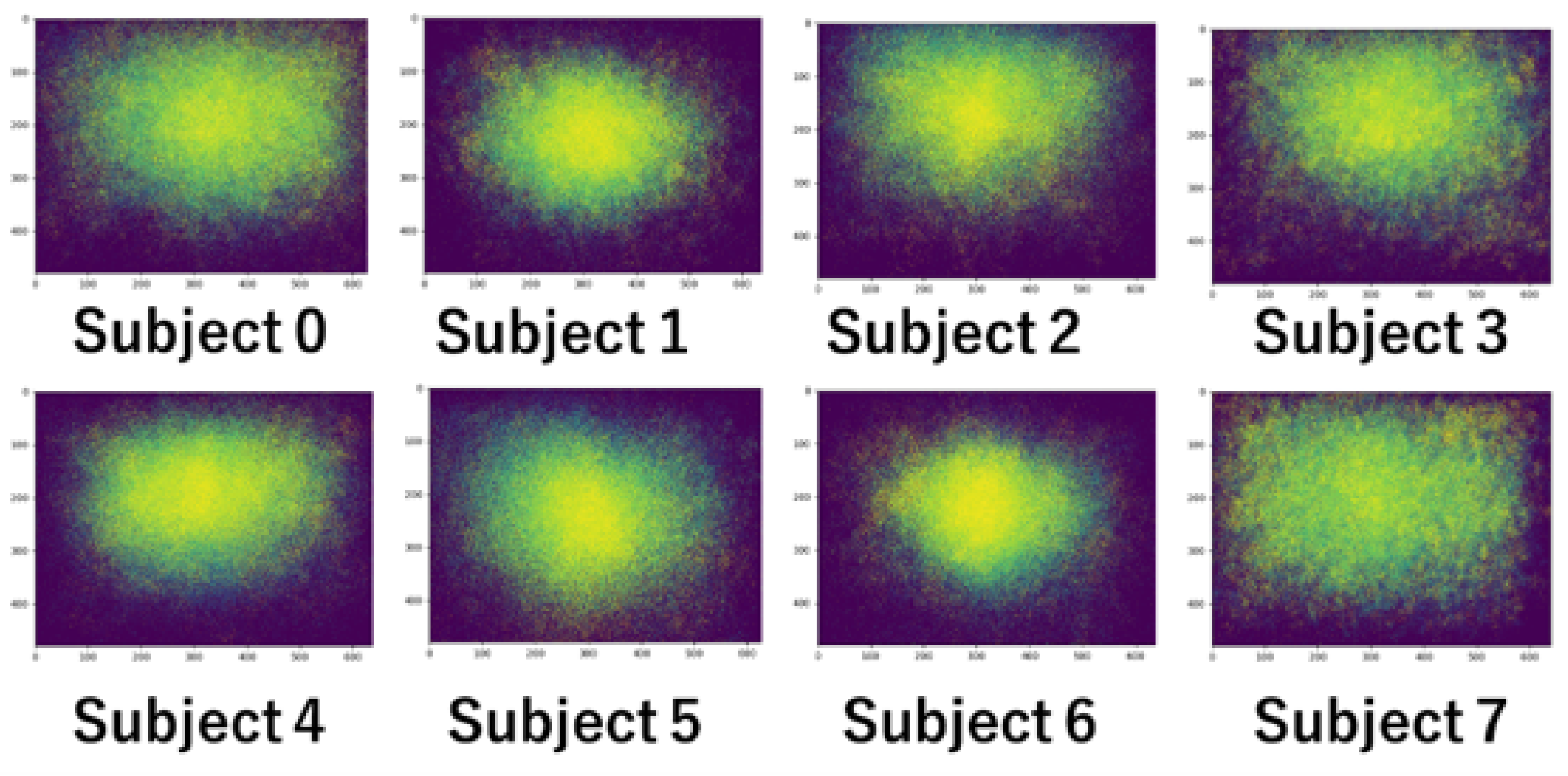
Figure 7.
Cosine Similarity between Subject PSMs
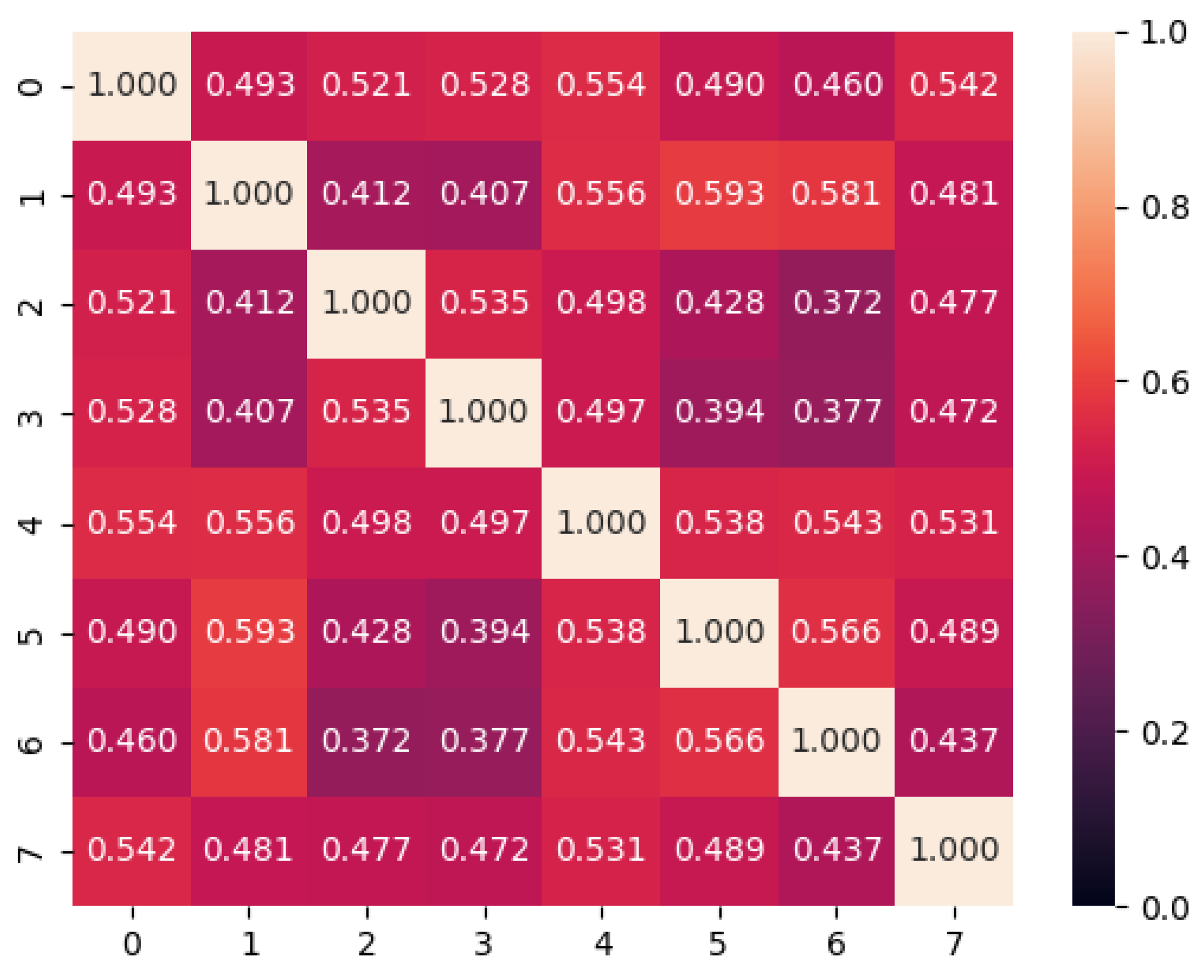
Figure 8.
Histgram of Subject Pupil Diameters
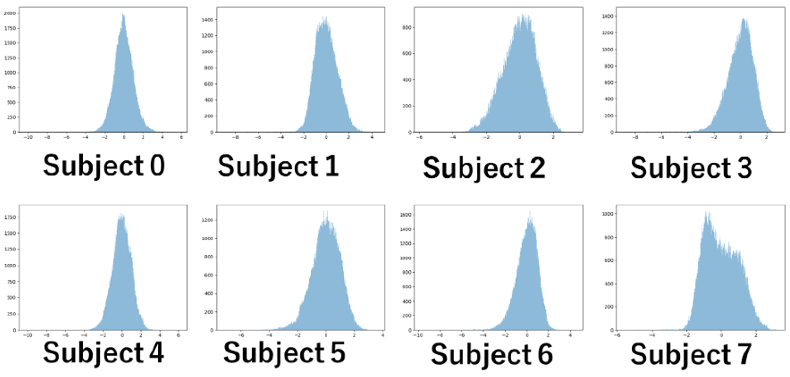
Figure 9.
QQ Plots of Subject Pupil Diameters
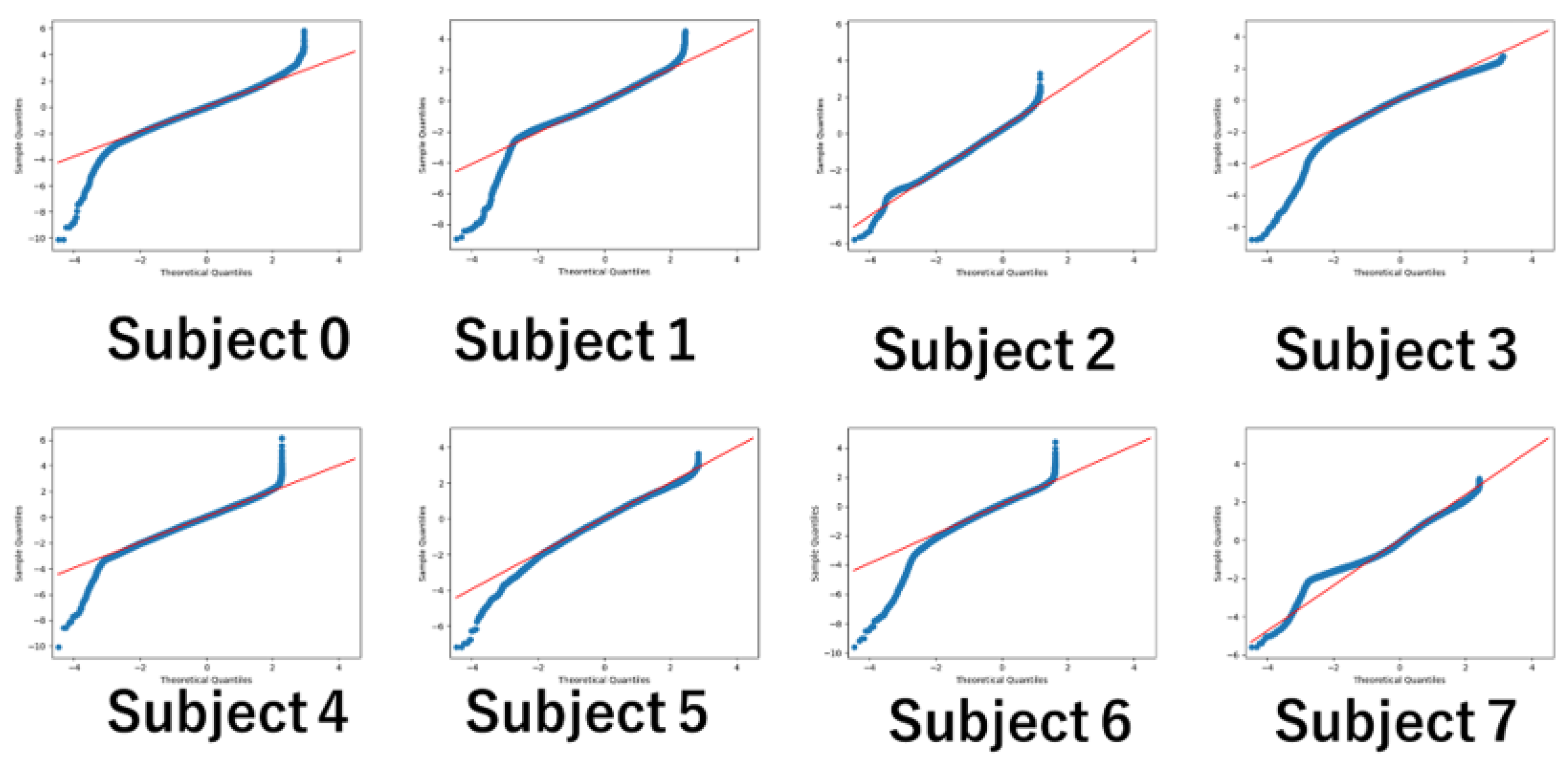
Figure 10.
Histgrams and QQ Plots of Subject 1 and 7 for Each day
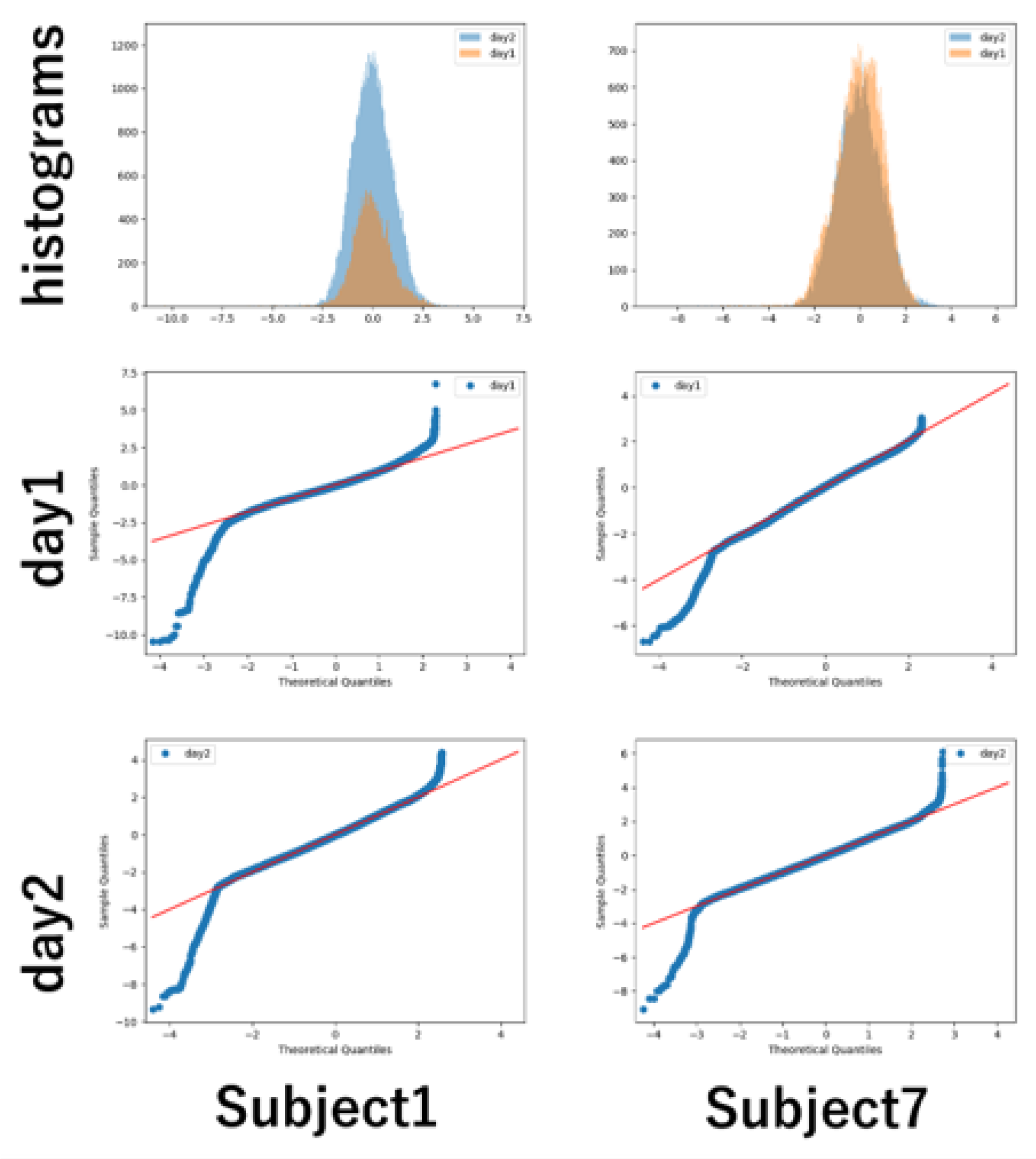
Figure 11.
Pupil Dilation of Each Subject per Image
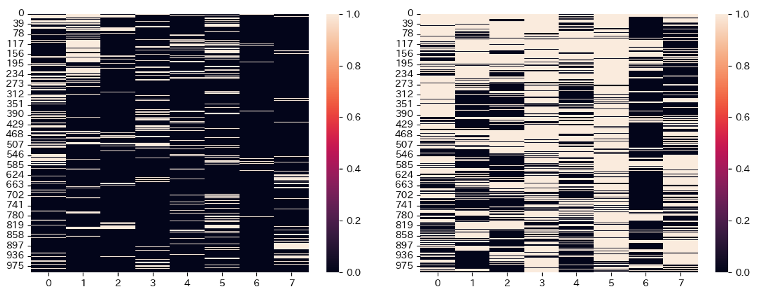
Figure 12.
Cosine Similarity of Each Subject’s Interest (Left: 1%, Right: 10%)
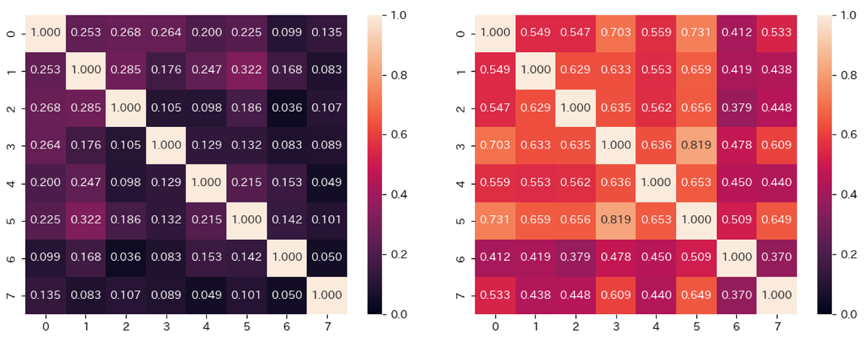
Figure 13.
Outputs of Model for Predicting Personal Gaze
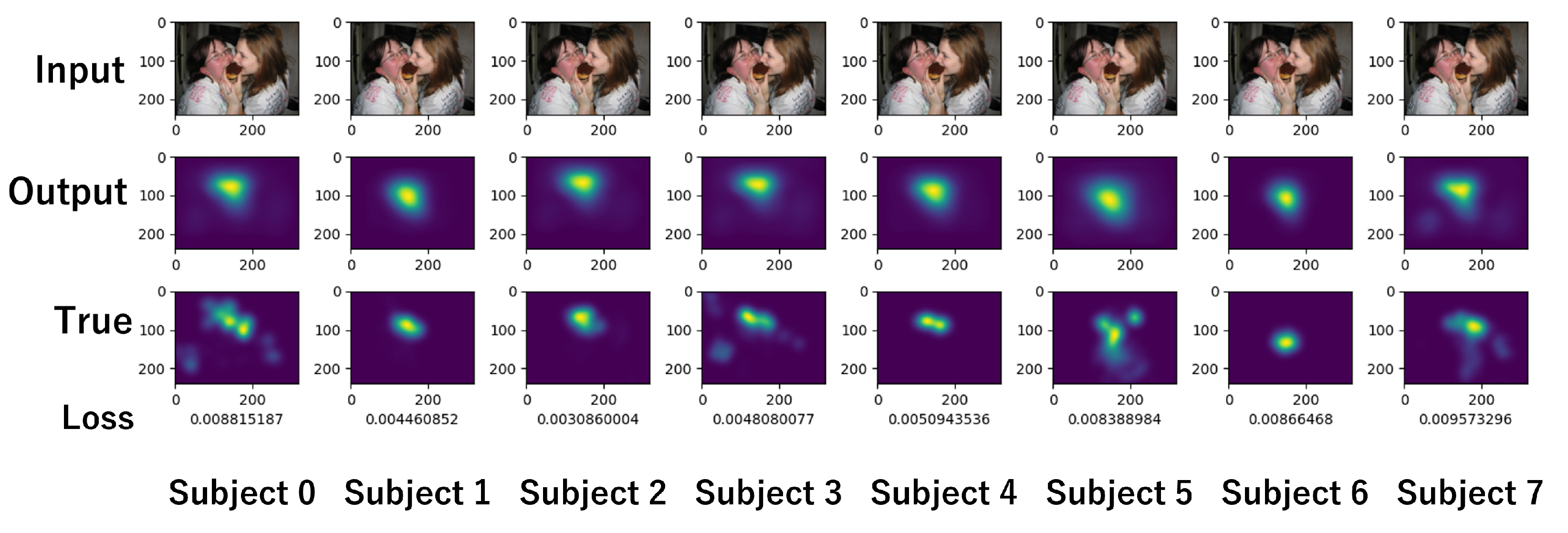
Figure 14.
Model to Verify Hypothesis
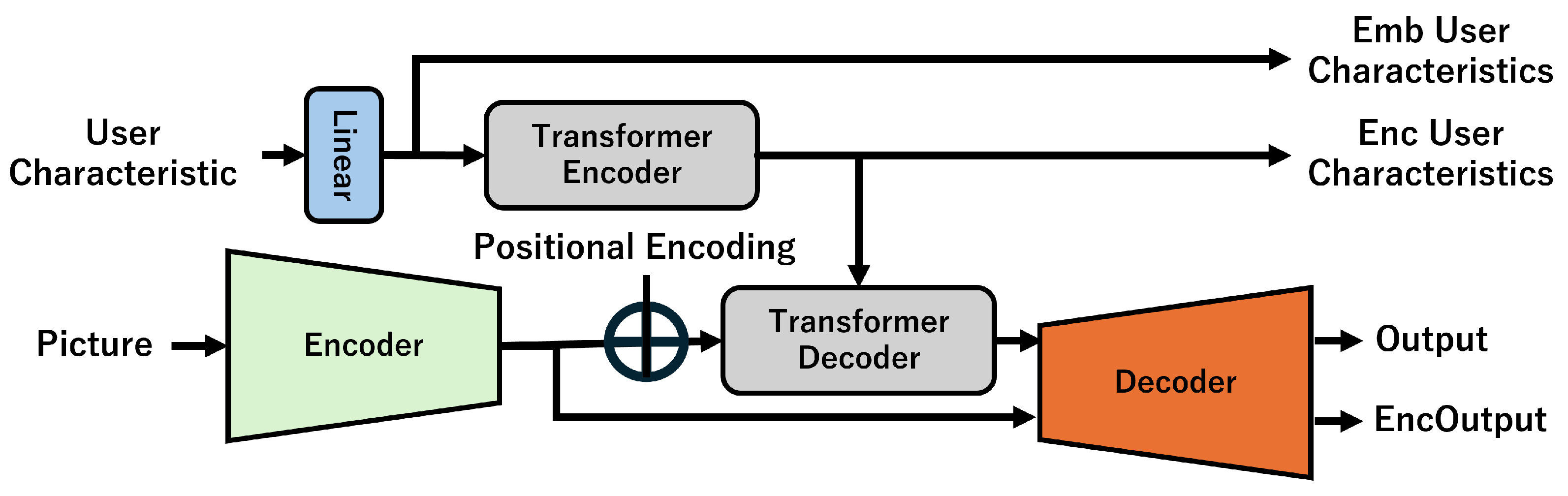
Figure 15.
Training from Random Initial Values
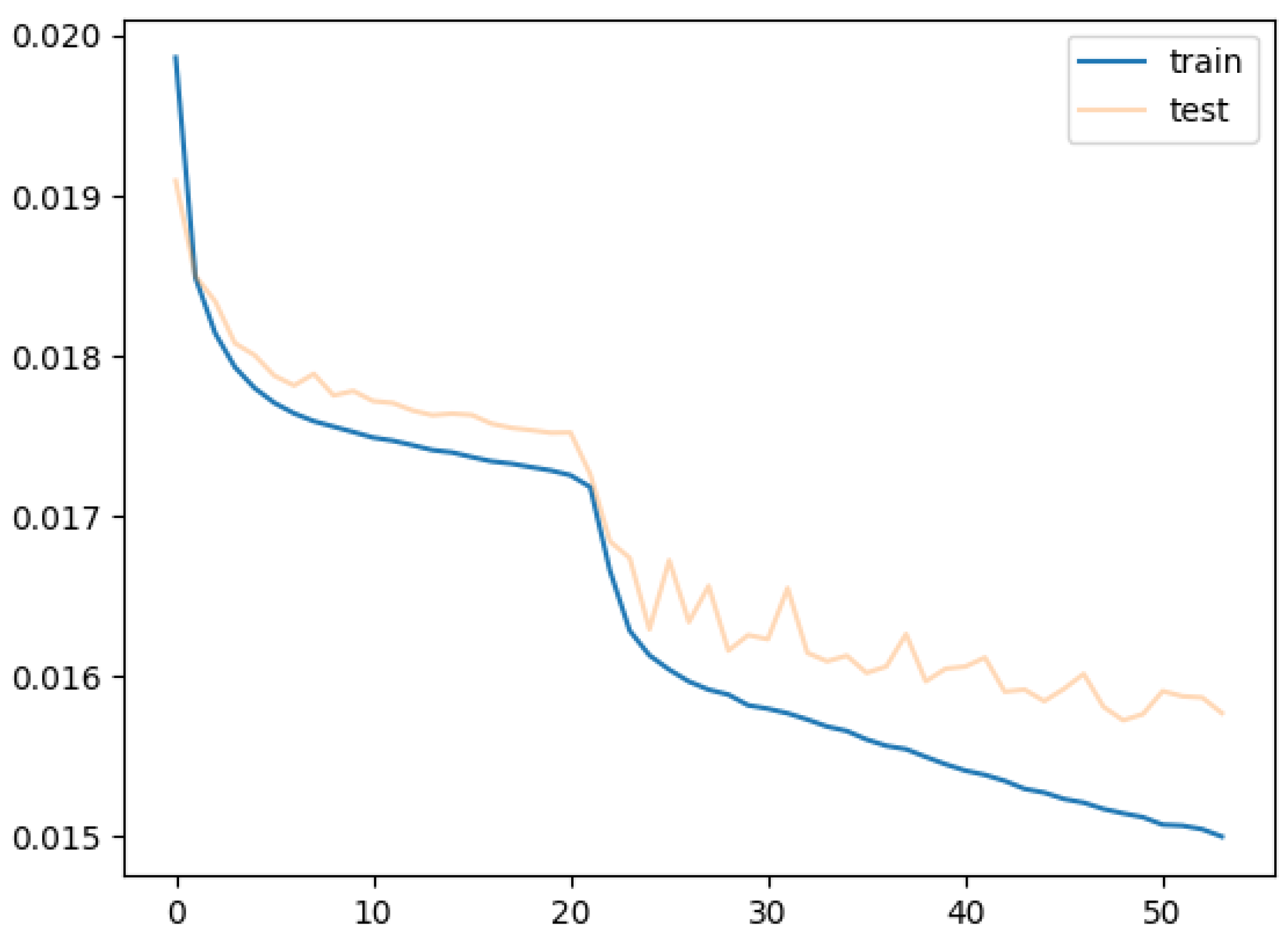
Figure 16.
Visualization at 20 epochs
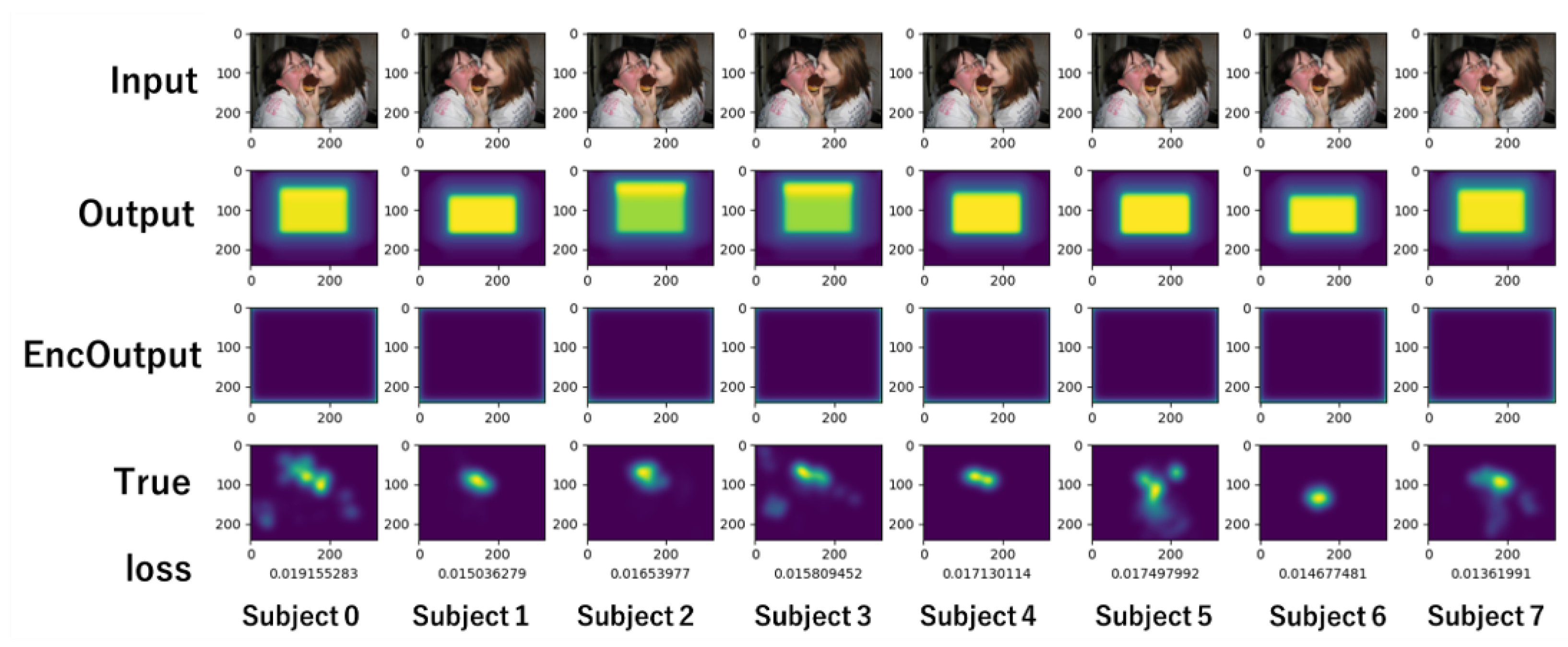
Figure 17.
Visualization at 53 epochs
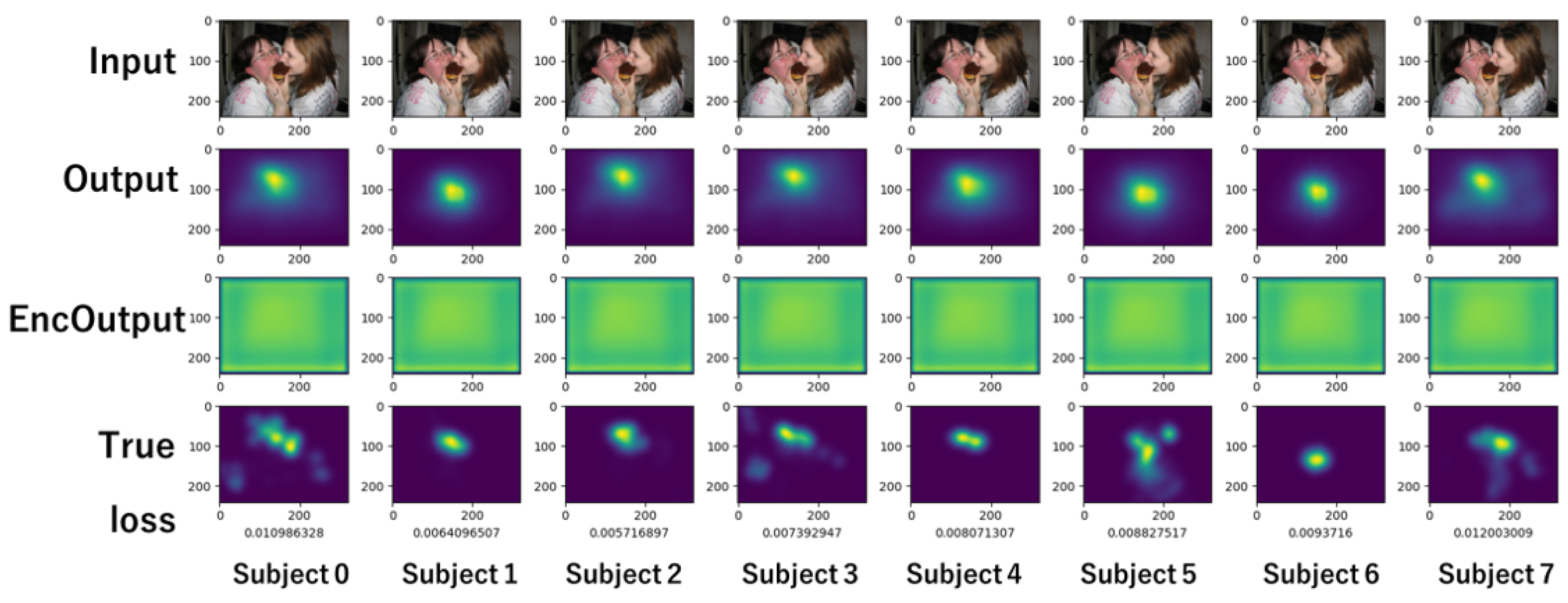
Figure 18.
Training Based on USM Parameters
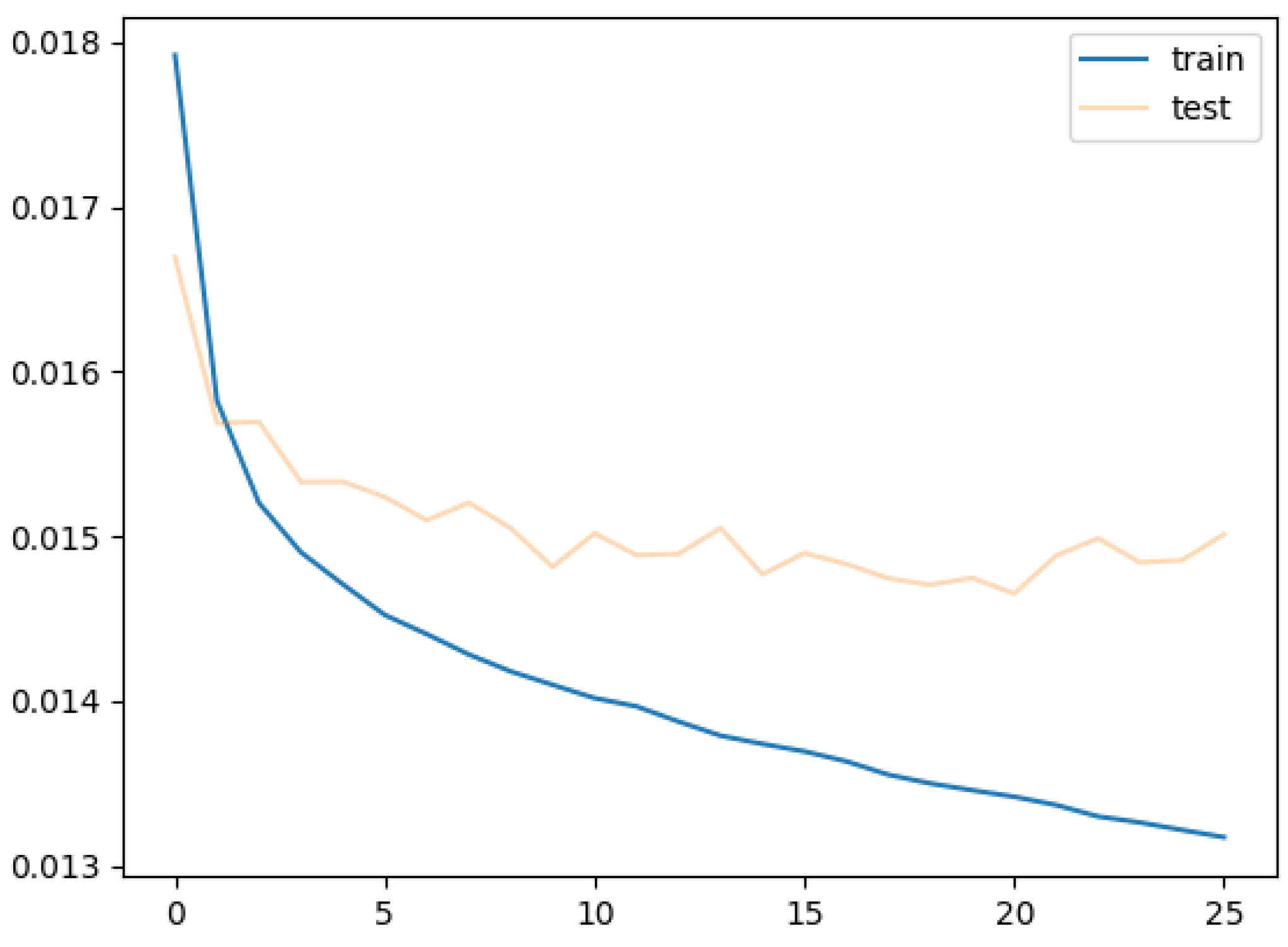
Figure 19.
Visualization of Training Results Based on USM Parameters
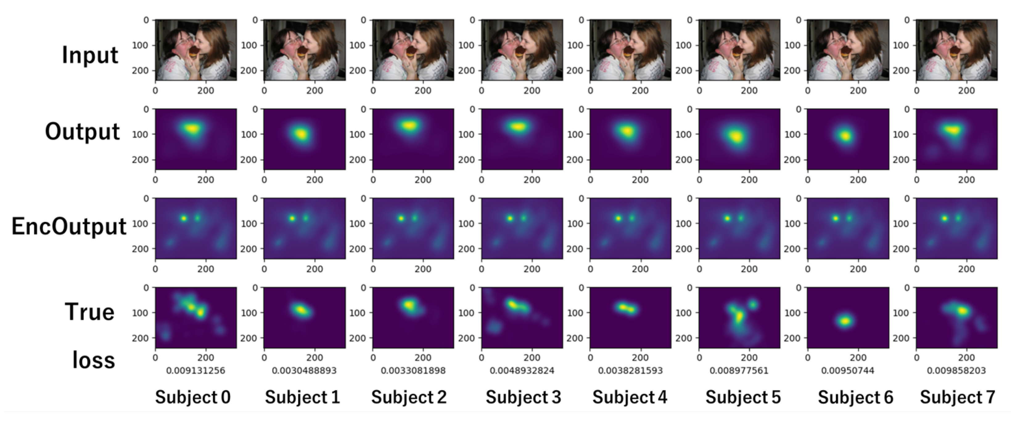
Figure 20.
Visualization of Model for USM
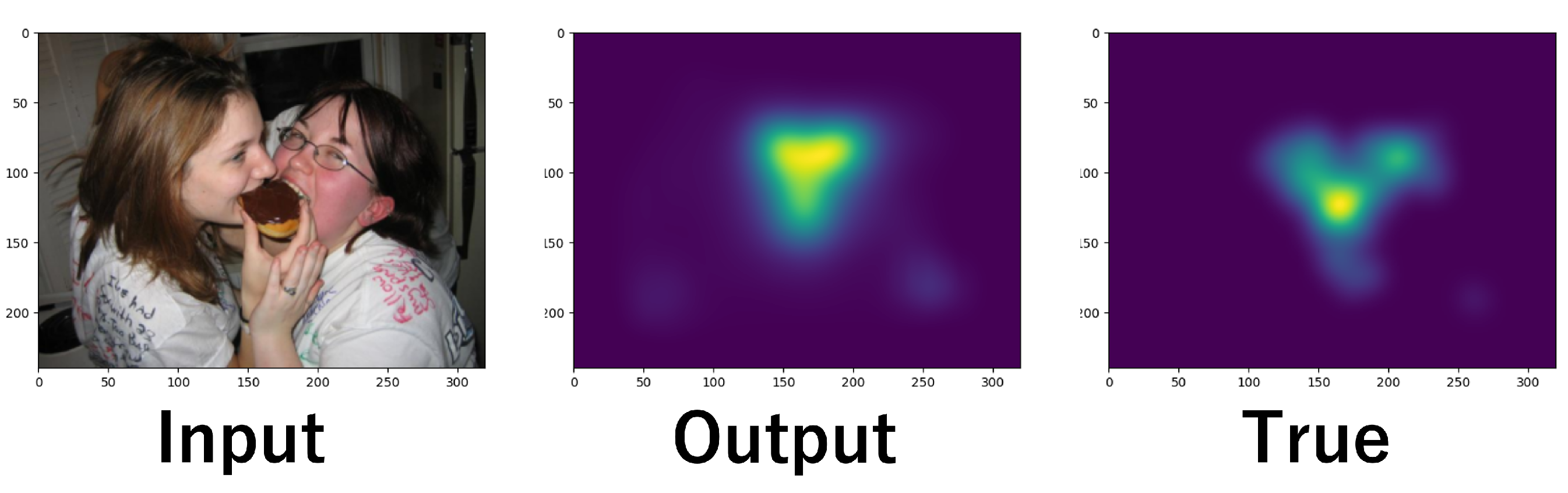
Figure 21.
Cosine Similarity between Each Subject in EncUserCharacteristics
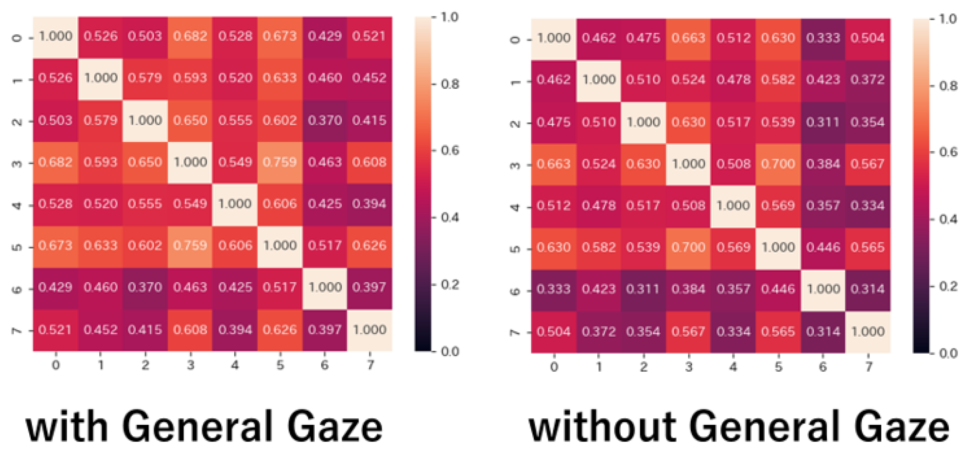

Table 1.
Layers of Encoder
| Layer | Depth | Kernel | Stride | Padding | Activation |
|---|---|---|---|---|---|
| Conv2D | 64 | 1*1 | 1 | 1 | ReLU |
| Conv2D | 64 | 3*3 | 1 | 1 | ReLU |
| MaxPool2D | 2*2 | 2 | 0 | ||
| Conv2D | 128 | 3*3 | 1 | 1 | ReLU |
| Conv2D | 128 | 3*3 | 1 | 1 | ReLU |
| MaxPool2D | 2*2 | 2 | 0 | ||
| Conv2D | 256 | 3*3 | 1 | 1 | ReLU |
| Conv2D | 256 | 3*3 | 1 | 1 | ReLU |
| Conv2D | 256 | 3*3 | 1 | 1 | ReLU |
| MaxPool2D | 2*2 | 2 | 0 | ||
| Conv2D | 512 | 3*3 | 1 | 1 | ReLU |
| Conv2D | 512 | 3*3 | 1 | 1 | ReLU |
| Conv2D | 512 | 3*3 | 1 | 1 | ReLU |
| MaxPool2D | 2*2 | 2 | 0 | ||
| Conv2D | 512 | 3*3 | 1 | 1 | ReLU |
| Conv2D | 512 | 3*3 | 1 | 1 | ReLU |
| Conv2D | 512 | 3*3 | 1 | 1 | ReLU |
Table 2.
Layers of Decoder
| Layer | Depth | Kernel | Stride | Padding | Activation |
|---|---|---|---|---|---|
| Conv2D | 512 | 3*3 | 1 | 1 | ReLU |
| Conv2D | 512 | 3*3 | 1 | 1 | ReLU |
| Conv2D | 512 | 3*3 | 1 | 1 | ReLU |
| UpSample | 2*2 | 2 | 0 | ||
| Conv2D | 512 | 3*3 | 1 | 1 | ReLU |
| Conv2D | 512 | 3*3 | 1 | 1 | ReLU |
| Conv2D | 512 | 3*3 | 1 | 1 | ReLU |
| UpSample | 2*2 | 2 | 0 | ||
| Conv2D | 256 | 3*3 | 1 | 1 | ReLU |
| Conv2D | 256 | 3*3 | 1 | 1 | ReLU |
| Conv2D | 256 | 3*3 | 1 | 1 | ReLU |
| UpSample | 2*2 | 2 | 0 | ||
| Conv2D | 128 | 3*3 | 1 | 1 | ReLU |
| Conv2D | 128 | 3*3 | 1 | 1 | ReLU |
| UpSample | 2*2 | 2 | 0 | ||
| Conv2D | 64 | 3*3 | 1 | 1 | ReLU |
| Conv2D | 64 | 3*3 | 1 | 1 | ReLU |
| Conv2D | 1 | 1*1 | 1 | 0 | ReLU |
Table 3.
Collected Data Items
| Data Item | Explanation |
|---|---|
| Timestamp | Elapsed Seconds from Image Presentation |
| Left Eye Gaze Coordinates | Coordinates based on the top left |
| Right Eye Gaze Coordinates | Coordinates based on the top left |
| Left Pupil Diameter | Left Eye Pupil Size |
| Right Pupil Diameter | Right Eye Pupil Size |
Table 4.
Accuracy of PSM
| Subject ID | sAUC | AUC-B |
|---|---|---|
| 0 | 0.9071156618680438 | 0.9419253886144336 |
| 1 | 0.9158976654517679 | 0.9641849007734729 |
| 2 | 0.9045685597027522 | 0.9468337457837294 |
| 3 | 0.9176894376891533 | 0.9469340783127931 |
| 4 | 0.8994813998914786 | 0.9462664041017854 |
| 5 | 0.8773627780413019 | 0.9286451929073957 |
| 6 | 0.9045921468163373 | 0.9553466929167967 |
| 7 | 0.9410767264429488 | 0.959907013306794 |
| mean | 0.908473046987973 | 0.94875542708965 |
Table 5.
Performance of Model to Predict General Gaze
| sAUC | AUC-B | NSS | CC |
|---|---|---|---|
| 0.8556327903801951 | 0.8622561397074704 | 1.707360242253475 | 0.8399891614959102 |
Table 6.
Optimal Layer Numbers of Encoder and Decoder of Transformer
| Enc/Dec | MSE Loss |
|---|---|
| 3/6 | 0.016044 |
| 3/9 | 0.016149 |
| 4/8 | 0.015959 |
| 4/9 | 0.015803 |
| 4/12 | 0.017498 |
| 6/6 | 0.016218 |
| 9/9 | 0.01603 |
Table 7.
Optimal Number of Heads
| Type/heads | MSE Loss |
|---|---|
| 1%/32 | 0.014936686 |
| 1%/64 | 0.014898729 |
| 1%/128 | 0.014857693 |
| 1%/256 | 0.014764848 |
| 10%/32 | 0.015030035 |
| 10%/64 | 0.01494549 |
| 10%/128 | 0.0149971135 |
| 10%/256 | 0.0147023015 |
| 10%/512 | 0.014754556 |
Table 8.
Performance of Model for Predicting Individual Gaze
| subject | sAUC | AUC-B | NSS | CC |
|---|---|---|---|---|
| 0 | 0.7500 | 0.7657 | 1.0255 | 0.4372 |
| 1 | 0.8312 | 0.8630 | 1.6853 | 0.5729 |
| 2 | 0.7534 | 0.7834 | 1.1055 | 0.4839 |
| 3 | 0.7443 | 0.7580 | 0.9887 | 0.4195 |
| 4 | 0.7912 | 0.8147 | 1.2609 | 0.5251 |
| 5 | 0.7968 | 0.8146 | 1.3225 | 0.5946 |
| 6 | 0.8254 | 0.8535 | 1.7067 | 0.5282 |
| 7 | 0.7145 | 0.7357 | 0.8504 | 0.3479 |
| mean | 0.7758 | 0.7986 | 1.2432 | 0.4887 |
Table 9.
Cosine Similarity of EmbUserCharacteristics with/without USM Parameters
| Subject | Cosine Similarity |
|---|---|
| 0 | 0.9148947 |
| 1 | 0.95943834 |
| 2 | 0.94265401 |
| 3 | 0.92215813 |
| 4 | 0.93176272 |
| 5 | 0.93883808 |
| 6 | 0.97130742 |
| 7 | 0.94247958 |
| mean | 0.9404416225 |
Table 10.
Cosine Similarity of EncUserCharacteristics with/without USM Parameters
| Subject | Cosine Similarity |
|---|---|
| 0 | 0.40764675 |
| 1 | 0.71327605 |
| 2 | 0.45038623 |
| 3 | 0.41545308 |
| 4 | 0.49677647 |
| 5 | 0.70966673 |
| 6 | 0.75337164 |
| 7 | 0.45110928 |
| mean | 0.5497107787500001 |
Disclaimer/Publisher’s Note: The statements, opinions and data contained in all publications are solely those of the individual author(s) and contributor(s) and not of MDPI and/or the editor(s). MDPI and/or the editor(s) disclaim responsibility for any injury to people or property resulting from any ideas, methods, instructions or products referred to in the content. |
© 2026 by the authors. Licensee MDPI, Basel, Switzerland. This article is an open access article distributed under the terms and conditions of the Creative Commons Attribution (CC BY) license (http://creativecommons.org/licenses/by/4.0/).
Copyright: This open access article is published under a Creative Commons CC BY 4.0 license, which permit the free download, distribution, and reuse, provided that the author and preprint are cited in any reuse.


