
Submitted:
13 March 2026
Posted:
16 March 2026
You are already at the latest version
Abstract
To address the issue of low accuracy of faulty feeder detection methods based on single fault characteristics, a faulty feeder detection method for resonant grounding systems based on multiple transient characteristics fusion was proposed. First, the transient zero-sequence current fault characteristics of both faulty and healthy feeders during single-phase-to-ground (SPG) faults were analyzed. Then, the transient zero-sequence current of each feeder was decomposed into intrinsic mode functions (IMFs) using variational mode decomposition (VMD), and a new signal was constructed by combining IMF1 and IMF2. Subsequently, transient energy and waveform similarity fault characteristics were extracted from the constructed signal, and a faulty feeder detection criterion based on multiple transient characteristics fusion was developed. Finally, extensive simulations and field data were used to verify the proposed faulty feeder detection method. The results demonstrated that the method was robust against fault resistance, fault inception angle, fault location, and noise, achieving high accuracy in faulty feeder detection. This method can be widely applied to detect faulty feeders in resonant grounding systems.
Keywords:
Resonant grounding system
; single-phase-to-ground
; faulty feeder detection
; variational mode decomposition
; transient energy
; waveform similarity
1. Introduction
With the continuous advancement of distribution automation, the demand for high power supply reliability in distribution networks is increasing. Distribution networks in China, Japan, and many European countries commonly employ the neutral non-effective grounding method [1]. Due to the weak grounding fault current during single-phase-to-ground (SPG) faults, detecting the faulty feeder in such systems is challenging, especially in resonant grounding systems [2,3]. SPG faults account for approximately 80% of faults in distribution networks [4,5], and if the faulty feeder is not accurately identified and promptly isolated, these faults can lead to severe consequences such as phase-to-phase short circuits and fire hazards [6]. Therefore, developing a highly accurate and reliable method for detecting SPG faulty feeders is crucial to ensuring power supply reliability in distribution networks.
In recent years, numerous faulty feeder detection techniques have emerged, primarily categorized into feature-analysis-based methods [1,3,7,8,9,10,11,12,13,14,15,16,17,18,19,20,21] and artificial-intelligence-based methods [4,5,6,22,23,24,25]. Feature-analysis-based methods are further divided into steady-state methods [1,7,8,9,10] and transient methods [3,11,12,13,14,15,16,17,18,19,20,21]. Steady-state methods based on fundamental waves are not applicable to resonant grounding systems, and the fault detection accuracy of steady-state methods based on harmonics is easily affected by the type of fault. Consequently, steady-state methods are rarely used in practical resonant grounding systems. Artificial-intelligence-based methods utilize advanced technologies such as convolutional neural networks, multi-evidence fusion, image processing, and particle swarm optimization algorithms to detect faulty feeders by integrating multiple fault characteristics. The accuracy of faulty feeder detection in these methods depends on the range of fault types included in the fault samples, and their generalization ability is limited. Therefore, the practical application of these methods requires further investigation.
Transient methods utilize advanced modern signal processing techniques, such as the fast Fourier transform (FFT), wavelet transform, Hilbert-Huang transform, empirical mode decomposition (EMD), and variational mode decomposition (VMD), to decompose transient zero-sequence current signals, extract fault characteristics (e.g., transient amplitude, energy, or polarity), and achieve faulty feeder detection. Due to the large amplitude and distinct characteristics of transient zero-sequence currents compared to steady-state zero-sequence currents, transient methods have become a prominent research focus. In [3], transient currents excluding fundamental frequency components were used to generate two fault indicators: transient energy within the first half power cycle and cosine similarity after the first half power cycle. The faulty feeder was identified based on the cumulative density function calculated from these two fault indicators. In [11], FFT was applied to calculate the fundamental components (FC), and faulty feeder detection was performed by obtaining transient zero-sequence current signals through subtracting the FC. However, these methods struggle to achieve accurate faulty feeder detection when transient zero-sequence currents are severely affected by noise interference. In [12], Flavio et al. presented a wavelet coefficient energy-based analysis for real-time fault-induced transient detection. In [13], Gao et al. utilized the empirical wavelet transform (EWT) to decompose differential faulty energy and adaptively selected the feature component with the largest permutation entropy. They employed a permutation variance index, constructed based on the sample point number and feature component energy, to detect high-impedance faults. Nevertheless, the accuracy of faulty feeder detection methods based on wavelet transform depends heavily on the choice of the mother wavelet function. In [14], Guo et al. used the Hilbert-Huang transform to decompose currents of all feeders connected to the bus into intrinsic mode functions (IMFs), detecting the faulty feeder by comparing the instantaneous amplitude of the first IMF. In [15], Wang et al. proposed a faulty feeder detection algorithm combining complete ensemble empirical mode decomposition with adaptive noise and Hilbert transform to construct a multi-criteria comprehensive voting method. However, the accuracy of these faulty feeder detection methods is susceptible to mode mixing and end effects.
To overcome the limitations of the aforementioned transient methods, the variational mode decomposition (VMD) algorithm has been applied to faulty feeder detection. In [17], Wang et al. proposed a high-impedance faulty feeder detection method that combined VMD with the Teager-Kaiser energy operator algorithm, utilizing VMD to extract the high-frequency components of transient zero-sequence currents. In [18], Wang et al. employed VMD to eliminate interference from high-frequency components and extracted the low-frequency characteristic modes of the transient zero-sequence current of each feeder to detect faults. However, neither of these methods fully exploits the characteristics of both the high-frequency and low-frequency components of transient zero-sequence currents. To address this limitation, this paper proposes a faulty feeder detection method based on multiple transient characteristics fusion.
We propose a faulty feeder detection method based on the transient energy and waveform similarity of transient zero-sequence currents. The main contributions are as follows:
- • We utilized VMD to decompose the transient zero-sequence current signals, removed the highest-frequency IMF, and then reconstructed a new transient zero-sequence current signal using the remaining IMFs. Subsequently, we calculated the transient energy of the reconstructed zero-sequence current signal.
- • We selected the three feeders with the largest transient energy, calculated their waveform similarities individually, and developed a faulty feeder detection criterion based on transient waveform similarity.
- • We verified the proposed faulty feeder detection method using both simulation data and field fault current data. The results demonstrate that the method can reliably and accurately identify the faulty feeder.
2. Fault Characteristics Analysis of Transient Zero-Sequence Currents
Based on the third-order equivalent circuit of SPG faults in resonant grounding systems established in [20], the equivalent circuit of the resonant grounding system when feeder n experiences an SPG fault is shown in Figure 1 [3,21]. uf (t) represents the equivalent virtual voltage source, it has the same magnitude but opposite phase relative to the pre-fault phase-to-ground voltage at the fault point. R denotes the equivalent resistance, which is the sum of the line-mode resistance, zero-mode resistance upstream of the fault point on the faulty feeder, and three times the fault resistance. L denotes the equivalent inductance, which is the sum of the line-mode inductance and zero-mode inductance upstream of the fault point on the faulty feeder. Lp represents the zero-sequence equivalent inductance of the Petersen coil, equal to three times the Petersen coil inductance. C0j denotes the zero-sequence distributed capacitance to ground of feeder j (j=1, …, n). I0f is zero-sequence current at the fault point. I0j represents the zero-sequence current of feeder j (j=1, …, n). I0Cn is the zero-sequence distributed capacitance current to ground of the faulty feeder n. iLp is the current through the Petersen coil.
When a low-impedance grounding fault occurs, the inductive reactance of the Petersen coil is much greater than the capacitive reactance of the capacitors; therefore, the impact of the Petersen coil on the transient zero-sequence current can be neglected [3,21]. The zero-sequence current i0n in the faulty feeder n can be calculated as follows [3]:
where i0n_FFC and i0n_TC are the fundamental frequency components (FFCs) and transient components (TCs) of i0n, respectively; Um is the peak value of uf; C0Σ is the sum of zero-sequence distributed capacitances to ground of all feeders; ω0 is the fundamental angular frequency; φ is the fault inception angle; δ is the damping ratio, defined as δ=Rf/(2L); and ωf is the resonant angular frequency of the transient process, defined as , A1 =1/(ω0ωfLC0Σ)sinφ+δ/ωfcosφ.
From Equations (1) and (2), i0n and i0k consist of two components: one is the FFCs, the other is the TCs. The direction of the TCs of the transient zero-sequence current in the faulty feeder is opposite to that in the healthy feeder. Moreover, the amplitude of the TCs in the faulty feeder is relatively large and significantly greater than that in the healthy feeder. In contrast, the FFCs of the transient zero-sequence current in the faulty feeder are similar to those in the healthy feeder. Therefore, faulty feeder detection can be effectively achieved by extracting the TCs.
When the grounding fault resistance Rf is high, Lp cannot be neglected, whereas L can be disregarded. If , the system is in an underdamping state. The zero-sequence current i0n in the faulty feeder n can be calculated as follows [3,21]:
where ; B1=-Asinθ; B2=-(δAsinθ+ω0Acosθ)/ωf; δ=1/(2RfC0Σ); ; .
If , the system is in an overdamping state. The zero-sequence current i0n in the faulty feeder n can be calculated as follows [21]:
where ; ; ; ; ; .
From Equations (3)–(6), the amplitudes and directions of the FFCs in both the faulty and healthy feeders are nearly identical. The amplitude of the TCs in the faulty feeder is slightly greater than that in the healthy feeder. Therefore, detecting the faulty feeder during high-impedance faults (HIFs) is very challenging.
As the Petersen coil is a dynamic component, its inductive current undergoes a transient process before reaching a steady-state value following an SPG fault. At the initial stage of SPG faults, the inductive current of the Petersen coil is very small, causing the coil to behave like a large inductance. According to equations (5) and (6), the amplitude of the FFCs in the faulty feeder is greater than that in the healthy feeders, and the direction of the FFCs in the faulty feeder is opposite to that in the healthy feeders during the initial stage of SPG faults. Therefore, faulty feeder detection can be achieved by extracting FFCs or TCs for any SPG faults.
3. Faulty Feeder Detection Criterion
3.1. Signal Decomposition Based on VMD
To achieve faulty feeder detection, it is first necessary to obtain the FFCs and TCs of transient zero-sequence current signals. Since the resonant frequency of TCs varies with different fault types and transient zero-sequence currents are susceptible to external interference, such as measurement errors, noise, and harmonic pollution, adaptive and non-recursive signal decomposition techniques must be employed. VMD is a recently developed multi-resolution technique for adaptive and non-recursive signal decomposition [26]. It iteratively decomposes the input signal to obtain K IMFs, making it highly suitable for faulty feeder detection based on transient zero-sequence currents.
The number of decomposition layers for VMD is generally set to three. Using VMD, the transient zero-sequence current of each feeder is decomposed into IMF1, IMF2, and IMF3. Among these, IMF1 represents the low-frequency components, including the FFCs; IMF2 captures the high-frequency components, primarily the TCs; and IMF3 corresponds to interference and residual components. Therefore, IMF1 and IMF2 are selected as the characteristic IMFs, and the following signal is reconstructed:
where icj is the reconstructed signal of the j-th feeder; uj1 and uj2 is the expressions for IMF1 and IMF2 of the j-th feeder, respectively. The reconstructed signal contains both the FFCs and the TCs, while eliminating interference signals, and can be used for faulty feeder detection.
icj = u1j+u2j,
Due to the distinct fault characteristics of the transient zero-sequence current signal in the faulty feeder during the initial stage of SPG faults, the data window for transient zero-sequence currents used in faulty feeder detection is selected as the first quarter of the power cycle.
3.2. Transient Energy Based Faulty Feeder Detection Criterion
The waveforms of the IMFk generated by different types of grounding faults vary significantly, making it challenging to calculate the amplitude of the reconstructed signal icj directly. Therefore, the transient energy of the reconstructed signal icj during the first quarter of the power cycle after SPG faults is used to represent its amplitude.
where Ej represents the transient energy of the j-th feeder; m denotes the index of the sampling point; M signifies the total number of sampling points within a quarter power cycle; icj(m) indicates the m-th sampled value of the reconstructed signal icj.
The proportion of transient energy contributed by each feeder to the total transient energy of all feeders connected to the bus varies. The transient energy proportion is calculated as follows:
where Δj represents the transient energy proportion of the j-th feeder; EΣ denotes the total energy of all feeders connected to the bus; and n signifies the total number of feeders.
The faulty feeder detection criterion based on transient energy is as follows: if the transient energy proportion of the j-th feeder satisfies the following inequality, then feeder j is identified as the faulty feeder; otherwise, it is considered healthy.
Δj>Δth,
where Δth represents the threshold for faulty feeder detection criteria, typically set within the range of 0.5<Δth <0.8.
3.3. Waveform Similarity Based Faulty Feeder Detection Criterion
At the initial stage of SPG faults, there is a significant difference in the transient zero-sequence current waveforms between the faulty feeder and the healthy feeders, while the transient zero-sequence current waveforms of the healthy feeders remain similar. Therefore, faulty feeder detection can be achieved by comparing the waveform similarity of the reconstructed transient zero-sequence current signals during the first quarter of a power cycle following an SPG fault. The waveform similarity is calculated as follows:
where ρjk represents the waveform similarity between the transient zero-sequence currents of the j-th and k-th feeders; icj(m) and ick(m) are the m-th sampled values of the reconstructed signal icj and ick, respectively.
To detect the faulty feeder, the waveform similarity coefficient ρj of the transient zero-sequence current of the j-th feeder is calculated as follows:
The proportion ηj of the waveform similarity coefficient for the j-th feeder relative to the total similarity coefficient of all feeders is calculated as follows:
where ηj represents the proportion of the waveform similarity coefficient for the j-th feeder, and ρΣ denotes the sum of the waveform similarity coefficients for all feeders connected to the bus.
The faulty feeder detection criterion based on waveform similarity is as follows: if the waveform similarity coefficient proportion ηj of the transient zero-sequence current in the j-th feeder satisfies the following inequality, then feeder j is identified as the faulty feeder; otherwise, it is considered healthy.
ηj < ηth,
where ηth represents the threshold value for the faulty feeder detection criterion, typically set within the range -0.2 < ηth < -0.05. If all feeders fail to meet the faulty feeder detection criteria, the fault is determined to be a bus fault.
3.4. Fusion-Based Faulty Feeder Detection Criterion
In various SPG fault scenarios in distribution networks, the amplitude or waveform characteristics of transient zero-sequence currents in the faulty feeder may not be distinctly evident. Consequently, the accuracy of faulty feeder detection based on a single fault characteristic tends to be relatively low. To improve detection accuracy, this paper proposes a faulty feeder detection method for resonant grounding systems based on multiple transient characteristics fusion, which integrates the amplitude and waveform characteristics of transient zero-sequence currents.
The faulty feeder detection method based on transient energy is less affected by interference and provides higher accuracy. However, in cases involving long feeders or HIFs, multiple feeders may exhibit large transient energy, making it difficult to accurately identify the faulty feeder. Additionally, when the transient zero-sequence current of a feeder is small, interference can cause a large waveform similarity error, leading to incorrect detection results using the waveform similarity-based method. To address these challenges, a fusion-based faulty feeder detection criterion has been developed: first, calculate the transient energy of the reconstructed signals for the transient zero-sequence currents of all feeders; then, select the three feeders with the highest transient energy. The waveform similarity comparison method is applied to these three feeders to identify the faulty feeder. If none of the feeders meet the detection criteria, the fault is determined to be a bus fault.
3.5. Flow Chart of Fusion-Based Faulty Feeder Detection Algorithm
The proposed faulty feeder detection method is implemented only when an SPG fault occurs. An SPG fault event is identified when the measured zero-sequence voltage U0 meets the following conditions:
U0 > kU N
where UN represents the rated phase voltage, and k denotes the reliability factor, which is typically set at 15%.
The flowchart of the proposed fusion-based faulty feeder detection algorithm is shown in Figure 2. The steps of the algorithm are as follows:
Step 1: Acquire the zero-sequence voltage at the bus in real time and calculate U0.
Step 2: If U0 > kUN is satisfied, start the faulty feeder detection algorithm.
Step 3: Record the transient zero-sequence current signal i0j in each feeder during the first quarter of the power cycle.
Step 4: Perform VMD decomposition on i0j to obtain uj1 and uj2.
Step 5: Calculate the reconstructed signal icj using Equation (7).
Step 6: Calculate Ej using Equation (8).
Step 7: Select the three feeders with the largest transient energy and calculate ρ12, ρ13, and ρ23 using Equation (11), respectively.
Step 8: Calculate ρj using Equation (12) and ηj using Equation (13).
Step 9: If ηj satisfies Inequality (14), feeder j is identified as the faulty feeder; otherwise, it is considered healthy. If none of the three feeders meet the faulty feeder detection criteria, the fault is determined to be a bus fault.
4. Simulation Analysis
4.1. Simulation Model
A typical radial distribution network model with four feeders has been developed in MATLAB, as shown in Figure 3. The lengths of the feeders are marked in the figure, and the parameters are listed in Table 1 [23]. In Figure 3, RL and LN represent the resistance and inductance of the Petersen coil connected to the Z-type grounding transformer. When the overcompensation degree is 8%, RL = 3 Ω, and LN = 294.3 mH. The system sampling frequency is set to 10 kHz.
4.2. Verification of Extracted Fault Characteristics
To verify the fault characteristics extracted in Section 2, the simulation model shown in Figure 3 is used to analyze the following two types of SPG faults.
4.2.1. Case 1
An SPG fault occurs at point k on the fourth feeder (F4), located 2 km from the bus, with a ground fault resistance Rg = 5 Ω, and a fault inception angles φ = 90°. The transient zero-sequence currents of F4 are shown in Figure 4. The number of modal decomposition layers K for VMD is set to 3, and the penalty factor α is set to 20000. The transient zero-sequence currents are decomposed using VMD, and the decomposed modal functions IMF1, IMF2, and IMF3 are presented in Figure 4. It can be observed that there are significant differences in the amplitude and waveform of IMF1 and IMF2 between the faulty feeder and the healthy feeders. The FFCs included in IMF1 are shown in Figure 5. As illustrated, there are notable differences between the FFCs of the faulty feeder and those of the healthy feeders during the initial stage of the SPG fault. Therefore, FFCs cannot be eliminated when using transient zero-sequence current for faulty feeder detection. The reconstructed signals using IMF1 and IMF2 for each feeder are shown in Figure 6. The figure demonstrates that there is a significant difference between the reconstructed signals of the faulty feeder and those of the healthy feeders under low impedance faults (LIFs), which can be used to reliably detect the faulty feeder.
4.2.2. Case 2
An SPG fault occurs at point k on F4, located 2 km from the bus, with a ground fault resistance Rg = 2000 Ω and a fault inception angles φ = 90°. The transient zero-sequence currents of F4 are shown in Figure 7. The decomposed modal functions IMF1, IMF2, and IMF3 obtained using VMD are also presented in Figure 7. It can be observed that there are significant differences in the amplitude and waveform of IMF1 between the faulty feeder and the healthy feeders. The FFCs included in IMF1 are shown in Figure 8. As illustrated, there are notable differences between the FFCs of the faulty feeder and those of the healthy feeders during the initial stage of the fault. Therefore, FFCs cannot be disregarded when using transient zero-sequence current for faulty feeder detection. The reconstructed signals using IMF1 and IMF2 for each feeder are shown in Figure 9. The figure reveals a significant difference between the reconstructed signals of the faulty feeder and those of the healthy feeders under HIFs, which can be used to reliably detect the faulty feeder. Consequently, whether the fault is an HIF or an LIF, the fault characteristics can be reliably extracted using the reconstructed signals.
4.3. Verification of the Proposed Faulty Feeder Detection Method
Many SLG fault scenarios under various fault conditions were simulated. These scenarios included different fault phases (phase A, B, or C), fault locations (at the bus or at 10%, 40%, 70%, or 90% along feeders 1–4), fault inception angles (0°, 45°, 90°, or 135°), and fault resistances (1 Ω, 10 Ω, 100 Ω, 1000 Ω, 2000 Ω, 3000 Ω, 4000 Ω, or 5000 Ω). A total of 1,632 fault scenarios were analyzed. In all cases, the proposed faulty feeder detection method reliably identified the faulted feeders or the faulty bus.
Several partial simulation data and faulty feeder detection results are presented in Table 2. Here, Fj represents the serial number of the faulty feeder, φ denotes the fault inception angle, Rg stands for the fault resistance, Ej signifies the transient energy, ρj indicates the waveform similarity coefficient, and ηj represents the waveform similarity coefficient proportion. By setting the threshold ηth to -0.1, all faulty feeder detection results are correct. Therefore, the proposed method can accurately detect the faulty feeder, and its reliability is not affected by fault conditions.
4.4. Noise Interference Test
White noise signals with signal-to-noise ratios (SNR) of 5 dB, 10 dB, and 20 dB were added to the transient zero-sequence currents in the fault scenarios described in Section 4.3 to verify the anti-interference capability of the proposed faulty feeder detection method. Figure 10 shows the zero-sequence currents and IMFs when an SPG occurs at 10% of F4 with a fault inception angle of 0°, a fault resistance of 1000 Ω, and an SNR of 5 dB. From the figure, it is evident that the transient zero-sequence current signals are severely affected by strong noise, making it difficult to distinguish the faulty feeder from the healthy feeder based solely on the noisy zero-sequence current signals. However, after applying VMD to the transient zero-sequence currents, the fault characteristics in IMF1 and IMF2 become apparent, enabling accurate detection of the faulty feeder. Partial simulation data with noise and the corresponding faulty feeder detection results are presented in Table 3. As shown, the proposed faulty feeder detection method is robust against noise and can accurately identify faulty feeders.
4.5. Compared with Existing Methods
To demonstrate the reliability advantage of the proposed faulty feeder detection method, we compared it with two methods introduced in [3] and [18]. Figure 11 shows the high-frequency components of transient zero-sequence currents during an SPG fault occurring at 10% of F4 with a fault inception angle of 90°, a fault resistance of 2000 Ω, and an SNR of 20 dB. In Figure 11, the difference in the first half-wave waveform between the faulty feeder and the healthy feeders is minimal. Consequently, detecting the faulty feeder based on the transient energy and waveform similarity of the high-frequency components of transient zero-sequence currents is challenging. Therefore, the faulty feeder detection method presented in [3] is ineffective under these conditions. Figure 12 illustrates the low-frequency components of zero-sequence currents during an SPG fault at 10% of F4 with a fault inception angle of 90°, a fault resistance of 3000 Ω, and an SNR of 5 dB. In Figure 12, the faulty feeder F4 exhibits the same polarity at the extreme values as the healthy feeders F1, F2, and F3. Thus, the faulty feeder detection method proposed in [18] fails in this scenario. Table 4 summarizes the accuracy rates of the faulty feeder detection methods proposed in this paper, as well as those in [3] and [18], based on the fault scenarios described in Section 4.4. As shown in Table 4, the proposed method achieves higher detection accuracy due to its ability to extract more effective fault characteristics.
4.6. Field Test
To verify the feasibility of the proposed faulty feeder detection method for field applications, five sets of field data were used for validation, and all results were accurate. At a substation in China with five feeders connected to a bus, the transient zero-sequence currents of each feeder during an SPG fault on feeder 4 are shown in Figure 13. The modal components IMF1, IMF2, and IMF3 obtained by VMD are shown in Figure 13. As illustrated, compared to the other healthy feeders, the fault characteristics in IMF1 and IMF2 of feeder 4 are clearly distinguishable. The signals reconstructed according to Equation (7) are shown in Figure 14. The faulty feeder detection results, summarized in Table 5, are all correct. Therefore, the proposed faulty feeder detection method is suitable for application in actual distribution networks.
5. Conclusion
In this study, we propose a faulty feeder detection method based on multiple transient characteristics fusion for resonant grounding systems. The main conclusions are as follows:
- • There are significant differences in both the amplitude and polarity of the low-frequency and high-frequency components of the transient zero-sequence current between the faulty feeder and the healthy feeder at the initial fault instant. Additionally, the fault characteristics of the fundamental components within the low-frequency components are also distinctive. Therefore, the low-frequency and high-frequency components extracted from transient zero-sequence currents can be effectively used to detect faulty feeders.
- • The fault characteristics of the signal, reconstructed from the low-frequency and high-frequency components of the transient zero-sequence current extracted through VMD decomposition, are clearly evident. By integrating the transient energy and waveform similarity of this reconstructed signal for faulty feeder detection, the method achieves high accuracy in identifying faulty feeders.
- • Through numerous simulations and field data tests, it has been demonstrated that the accuracy of the proposed faulty feeder detection method remains unaffected by fault resistance, inception angle, fault location, or noise. Compared to two existing faulty feeder detection methods, the proposed method exhibits superior accuracy and adaptability in detecting faulty feeders.
Author Contributions
Conceptualization, R.M.; methodology, R.M.; software, R.M.; validation, R.M.; formal analysis, R.M.; investigation, R.M.; resources, R.M., data curation, R.M.; writing—original draft preparation, R.M.; writing—review and editing, Q.P.; visualization, R.M.; supervision, Q.P.; project administration, R.M.; funding acquisition, R.M. All authors have read and agreed to the published version of the manuscript. All authors have read and agreed to the published version of the manuscript.
Funding
This research was funded by National College Students' Innovative Entrepreneurial Training Plan Program of China (Grant No. 202510429030).
Data Availability Statement
The original contributions presented in this study are included in the article. Further inquiries can be directed to the corresponding authors.
Conflicts of Interest
The authors declare no conflict of interest.
References
- Wei, M.; Shi, F.; Zhang, H.; Chen, W. Wideband Synchronous Measurement-Based Detection and Location of High Impedance Fault for Resonant Distribution Systems With Integration of DERs. IEEE Trans. Smart Grid 2023, 14, 1117–1134. [Google Scholar] [CrossRef]
- Wang, X.; Zhang, H.; Shi, F.; Wu, Q.; Terzija, V.; Xie, W.; Fang, C. Location of Single Phase to Ground Faults in Distribution Networks Based on Synchronous Transients Energy Analysis. IEEE Trans. Smart Grid 2020, 11, 774–785. [Google Scholar] [CrossRef]
- Wei, X.; Wang, X.; Gao, J.; Yang, D.; Wei, K.; Guo, L. Faulty Feeder Detection for Single-Phase-to-Ground Fault in Distribution Networks Based on Transient Energy and Cosine Similarity. IEEE Trans. Power Del 2022, 37, 3968–3978. [Google Scholar] [CrossRef]
- Yuan, J.; Xing, L.; Xue, M.; Chen, Q.; Hu, B.; Chen, X.; Liu, J.; Jiao, Z. A Highly Reliable Image-Recognition-Based Intelligent Fault Detection Method for Feeders Using Fully Convolutional Generative Adversarial Network. IEEE Trans. Smart Grid 2025, 16, 2278–2291. [Google Scholar] [CrossRef]
- Wei, X.; Yang, D.; Wang, X.; Wang, B.; Gao, J.; Wei, K. Faulty Feeder Detection Based on Fundamental Component Shift and Multiple-Transient-Feature Fusion in Distribution Networks. IEEE Trans. Smart Grid 2021, 12, 1699–1711. [Google Scholar] [CrossRef]
- Yuan, J.; Jiao, Z. Faulty-Feeder Detection for Single Phase-to-Ground Faults in Distribution Networks Based on Waveform Encoding and Waveform Segmentation. IEEE Trans. Smart Grid 2023, 14, 4100–4115. [Google Scholar] [CrossRef]
- Liu, P.; Du, S.; Sun, K.; Zhu, J.; Xie, D.; Liu, Y. Single-Line-to-Ground Fault Feeder Selection Considering Device Polarity Reverse Installation in Resonant Grounding System. IEEE Trans. Power Del. 2021, 36, 2204–2212. [Google Scholar] [CrossRef]
- Milioudis, A. H.; Andreou, G. T.; Labridis, D. P. Detection and Location of High Impedance Faults in Multiconductor Overhead Distribution Lines Using Power Line Communication Devices. IEEE Trans. Smart Grid 2021, 12, 894–902. [Google Scholar] [CrossRef]
- Lin, Y.-H.; Liu, C.-W.; Chen, C.-S. A new PMU-Based Fault Detection/Location Technique for Transmission Lines with Consideration of Arcing Fault Discrimination-Part I: Theory and Algorithms. IEEE Trans. Power Del. 2004, 19, 1587–1593. [Google Scholar] [CrossRef]
- Wang, B.; Geng, J.; Dong, X. High Impedance Fault Detection Based on Nonlinear Voltage-Current Characteristic Profile Identification. IEEE Trans. Smart Grid 2018, 9, 3783–3791. [Google Scholar] [CrossRef]
- Wang X., Wei X. Yang D., Song G., Gao J., Wei Y., Zeng Z., Peng W. Fault Feeder Detection Method Utilized Steady State and Transient Components Based on FFT Backstepping in Distribution Networks. Int. J. Elect. Power Energy Syst. 2020, 114, 105391.
- Costa, F. B. Fault-Induced Transient Detection Based on Real-Time Analysis of the Wavelet Coefficient Energy. IEEE Trans. Power Del. 2014, 29, 140–153. [Google Scholar] [CrossRef]
- Gao, J.; Wang, X.; Wang, X.; Yang, A.; Yuan, H.; Wei, X. A High-Impedance Fault Detection Method for Distribution Systems Based on Empirical Wavelet Transform and Differential Faulty Energy. IEEE Trans. Smart Grid 2022, 13, 900–912. [Google Scholar] [CrossRef]
- Guo, Z.; Yao, J. Hilbert-Huang Transform-Based Transient Busbar Protection Algorithm. IET Gen. Transmiss. Distrib. 2015, 9, 2032–2039. [Google Scholar] [CrossRef]
- Wang, X.; Gao, J.; Wei, X.; Zeng, Z.; Wei, Y.; Mostafa, K. Single Line to Ground Fault Detection in a Non-Effectively Grounded Distribution Network. IEEE Trans. Power Del. 2018, 33, 3173–3186. [Google Scholar] [CrossRef]
- Tang, T.; Zeng, X.; Huang, C.; Li, Z. Faulty Feeder Detection Based on the Composite Factors in Resonant Grounding Distribution System. Electric Power Syst. Res. 2020, 189, 106578. [Google Scholar] [CrossRef]
- Wang, X.; Gao, J.; Wei, X.; Song, G.; Wu, L.; Liu, J.; Zeng, Z.; Mostafa, K. High Impedance Fault Detection Method Based on Variational Mode Decomposition and Teager-Kaiser Energy Operators for Distribution Network. IEEE Trans. Smart Grid 2019, 10, 6041–6054. [Google Scholar] [CrossRef]
- Wang, X.; Gao, J.; Wei, X.; Guo, L.; Song, G.; Wang, P. Faulty Feeder Detection Under High Impedance Faults for Resonant Grounding Distribution Systems. IEEE Trans. Smart Grid 2023, 14, 1880–1895. [Google Scholar] [CrossRef]
- Yin, Z.; Wei, Z.; Sun, G.; Chen, S.; Zang, H. Unified Faulty Feeder Detection Criteria and High-Speed Protection Scheme for High Impedance Faults in Resonant Grounding MV Networks. IEEE Trans. Smart Grid 2025, 16, 3653–3665. [Google Scholar] [CrossRef]
- Xue, Y.; Li, J.; Xu, B. Transient Equivalent Circuit and Transient Analysis of Single-Phase Earth Fault in Arc Suppression Coil Grounded System. Proc. CESS 2015, 35, 5703–5714. [Google Scholar]
- Xue, Y.; Chen, X.; Song, H.; Xu, B. Resonance Analysis and Faulty Feeder Identification of High-Impedance Faults in a Resonant Grounding System. IEEE Trans. Power Del 2017, 32, 1545–1555. [Google Scholar] [CrossRef]
- Guo, M.; Zeng, X.; Chen, D.; Yang, N. Deep-Learning-Based Earth Fault Detection Using Continuous Wavelet Transform and Convolutional Neural Network in Resonant Grounding Distribution Systems. IEEE SENS. J. 2018, 18, 1291–1300. [Google Scholar] [CrossRef]
- Alenezi, M.; Anayi, F.; Packianather, M.; Shouran, M. A Hybrid Machine Learning Framework for Early Fault Detection in Power Transformers Using PSO and DMO Algorithms. Energies 2025, 18, 2024. [Google Scholar] [CrossRef]
- Moloi, K.; Davidson, I. High Impedance Fault Detection Protection Scheme for Power Distribution Systems. Mathematics 2022, 10, 4298. [Google Scholar] [CrossRef]
- Yu, X.; Cao, J.; Fan, Z.; Xu, M.; Xiao, L. Faulty Feeder Identification in Resonant Grounding Distribution Networks Based on Deep Learning and Transfer Learning. CSEE J. Power Energy Syst. 2023, 9, 2168–2178. [Google Scholar]
- Dragomiretskiy, K.; Zosso, D. Variational Mode Decomposition. IEEE Trans. Signal Process. 2014, 62, 531–544. [Google Scholar] [CrossRef]
Figure 1.
Zero-sequence equivalent circuit under SPG faults.
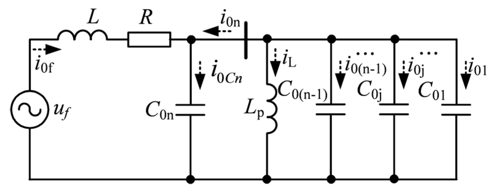
Figure 2.
Flow chart of fusion-based faulty feeder detection algorithm.
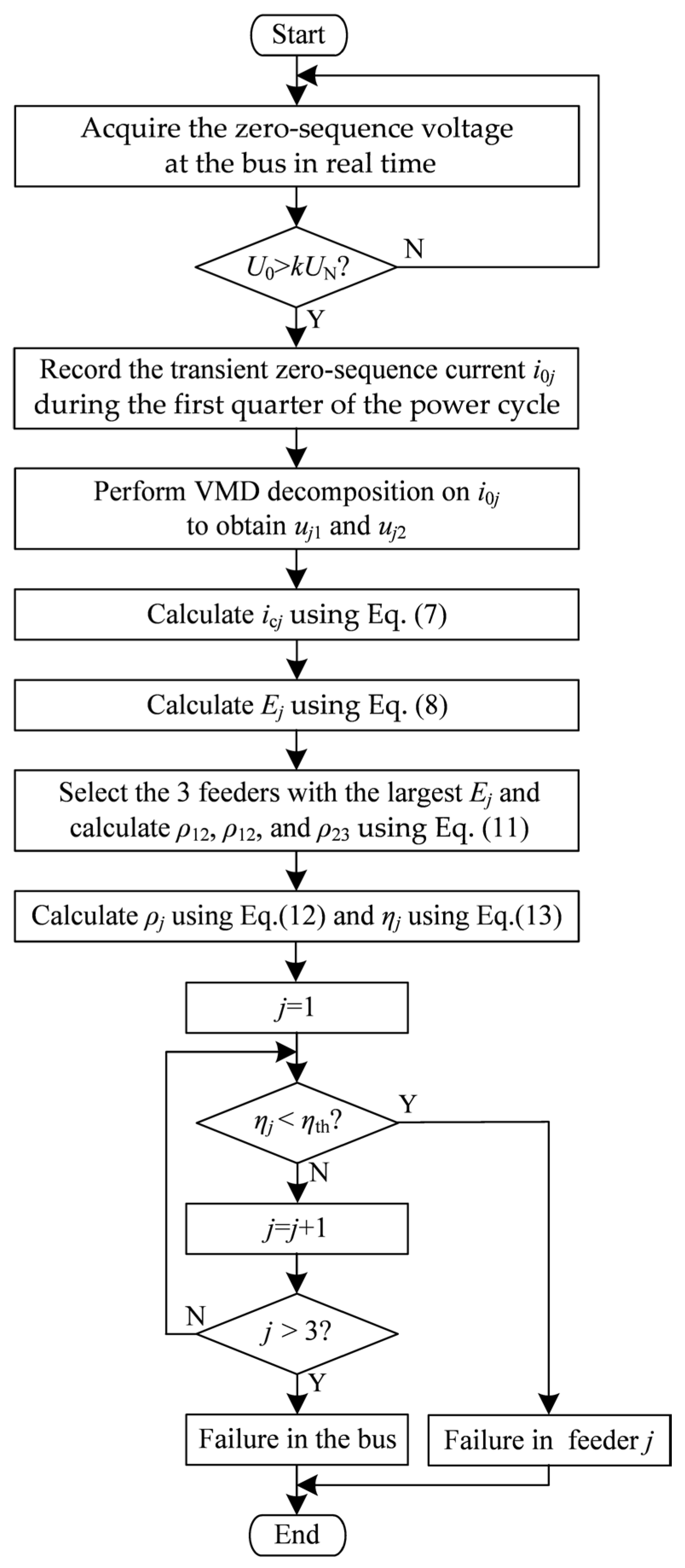
Figure 3.
Simulation mode.
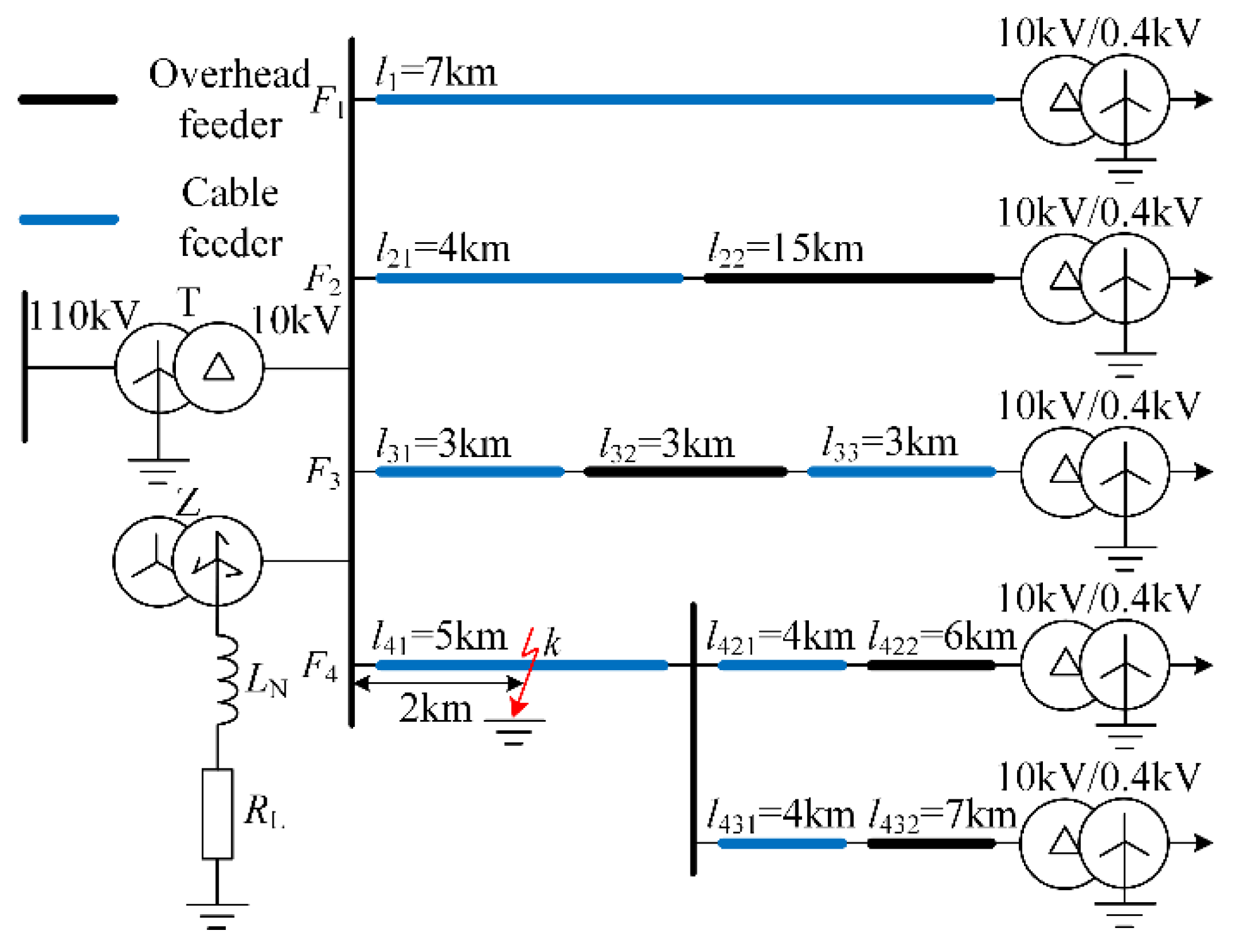
Figure 4.
VMD decomposition results of transient zero-sequence currents in case 1.
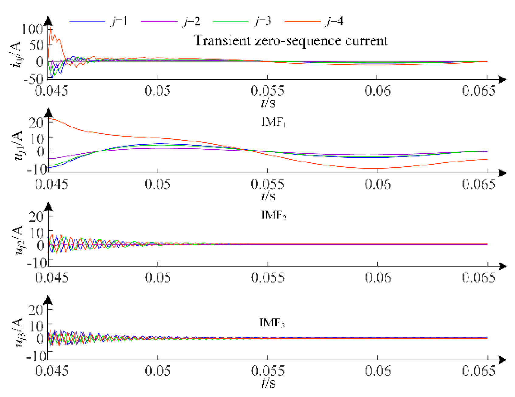
Figure 5.
FFCs of transient zero-sequence currents in case 1.
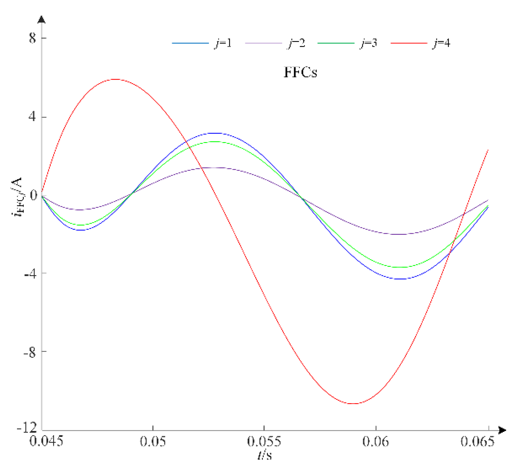
Figure 6.
Reconstruction signals in case 1.
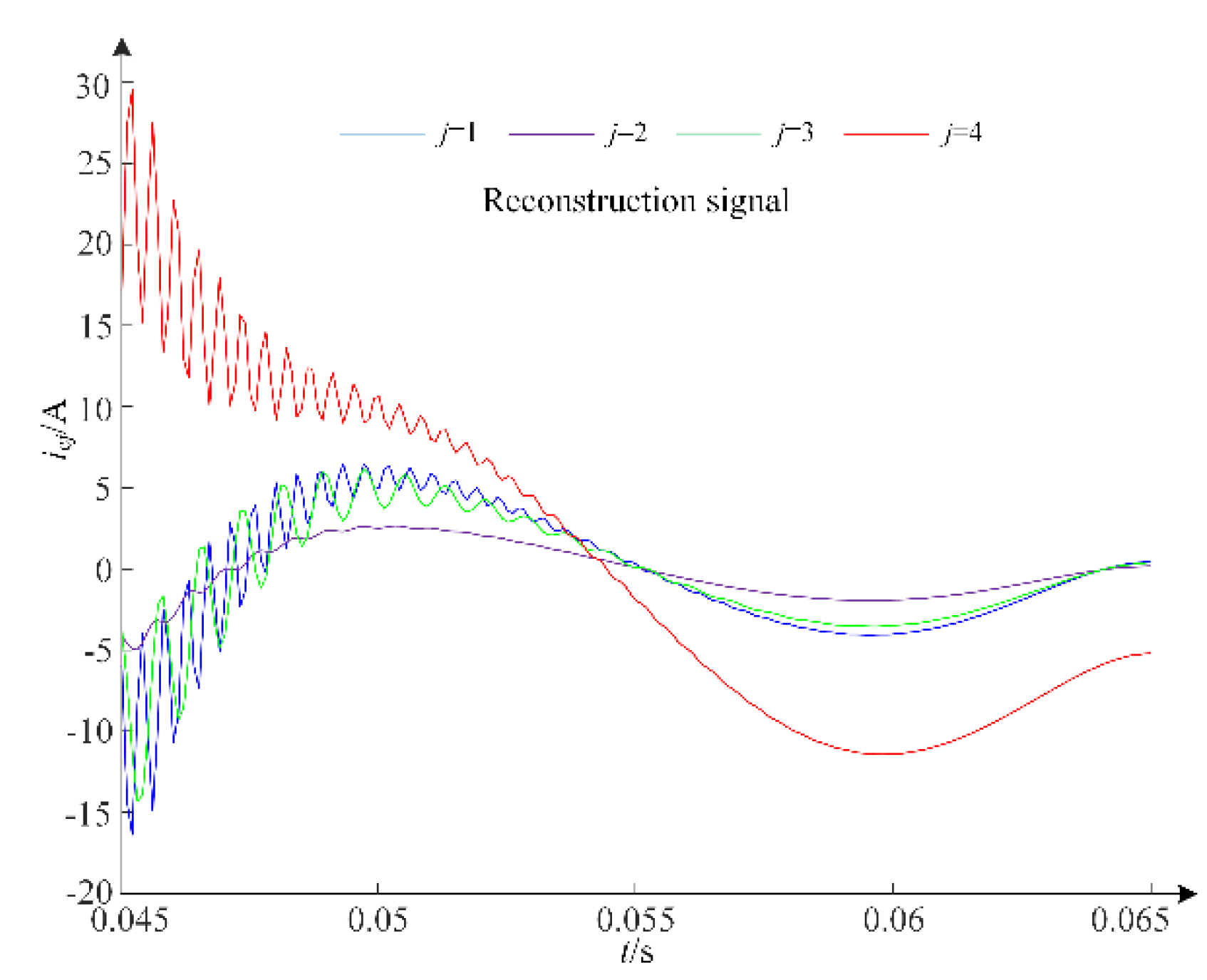
Figure 7.
VMD decomposition results of transient zero-sequence currents in case 2.
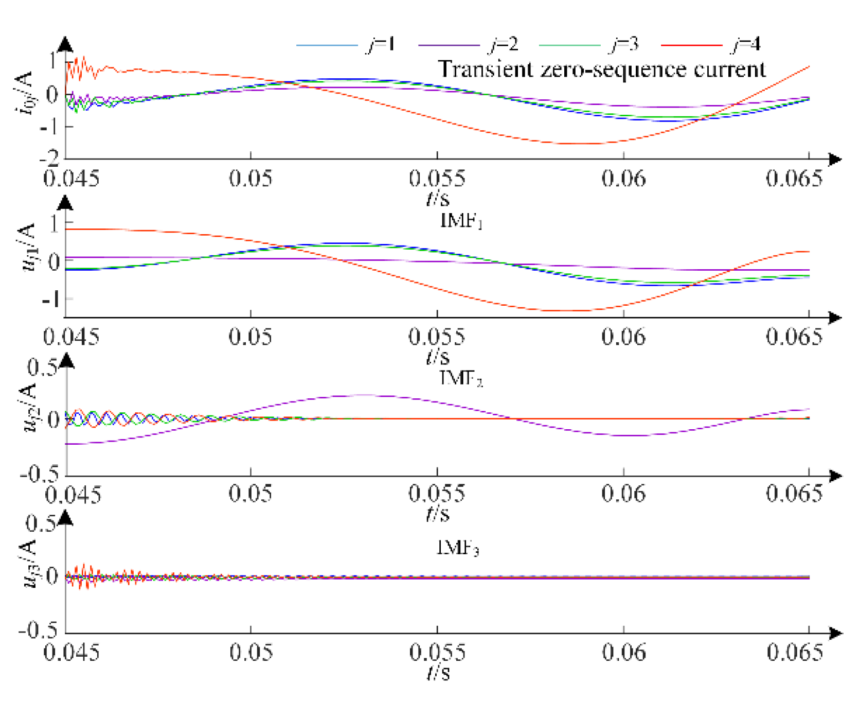
Figure 8.
FFCs of transient zero-sequence currents in case 2.
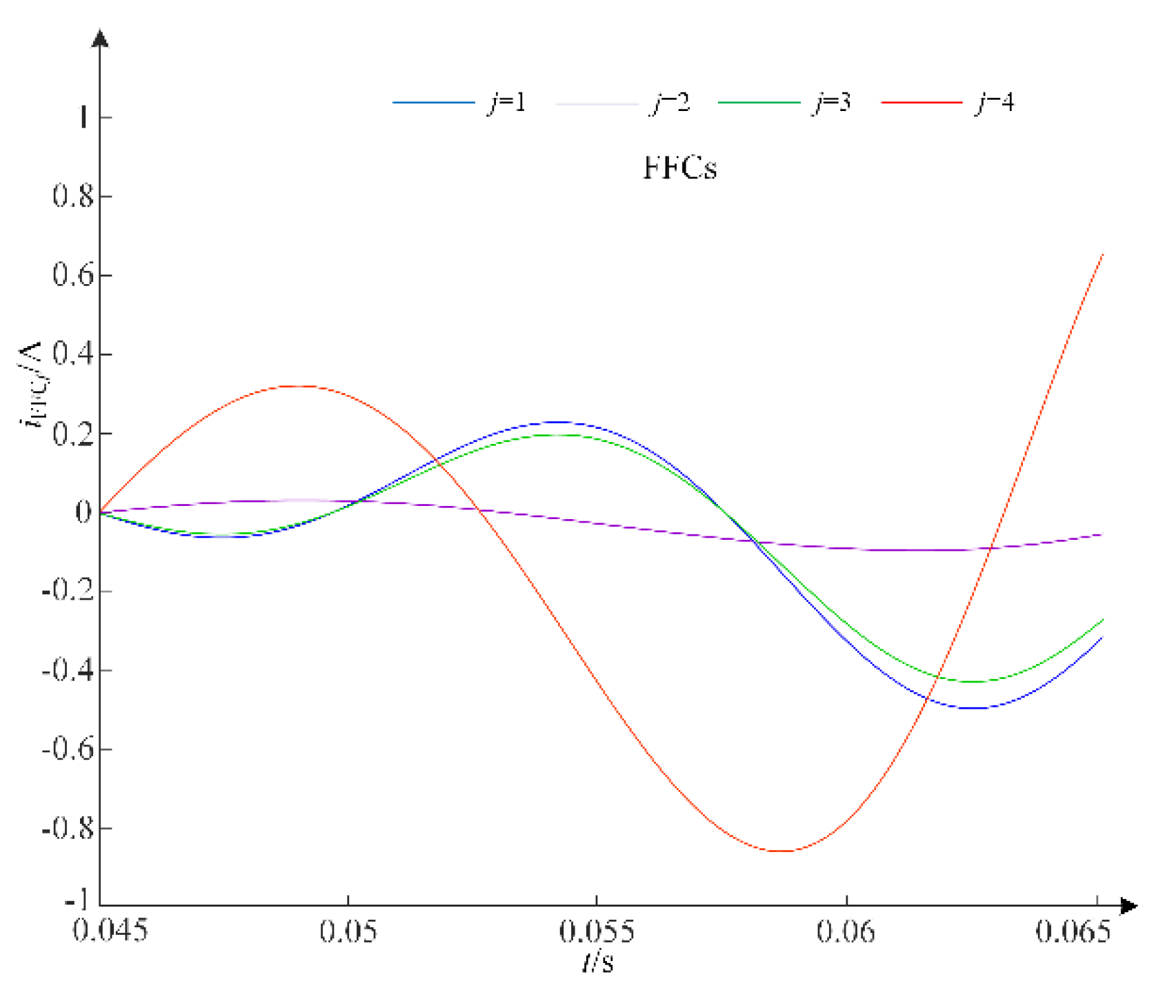
Figure 9.
Reconstruction signals in case 2.
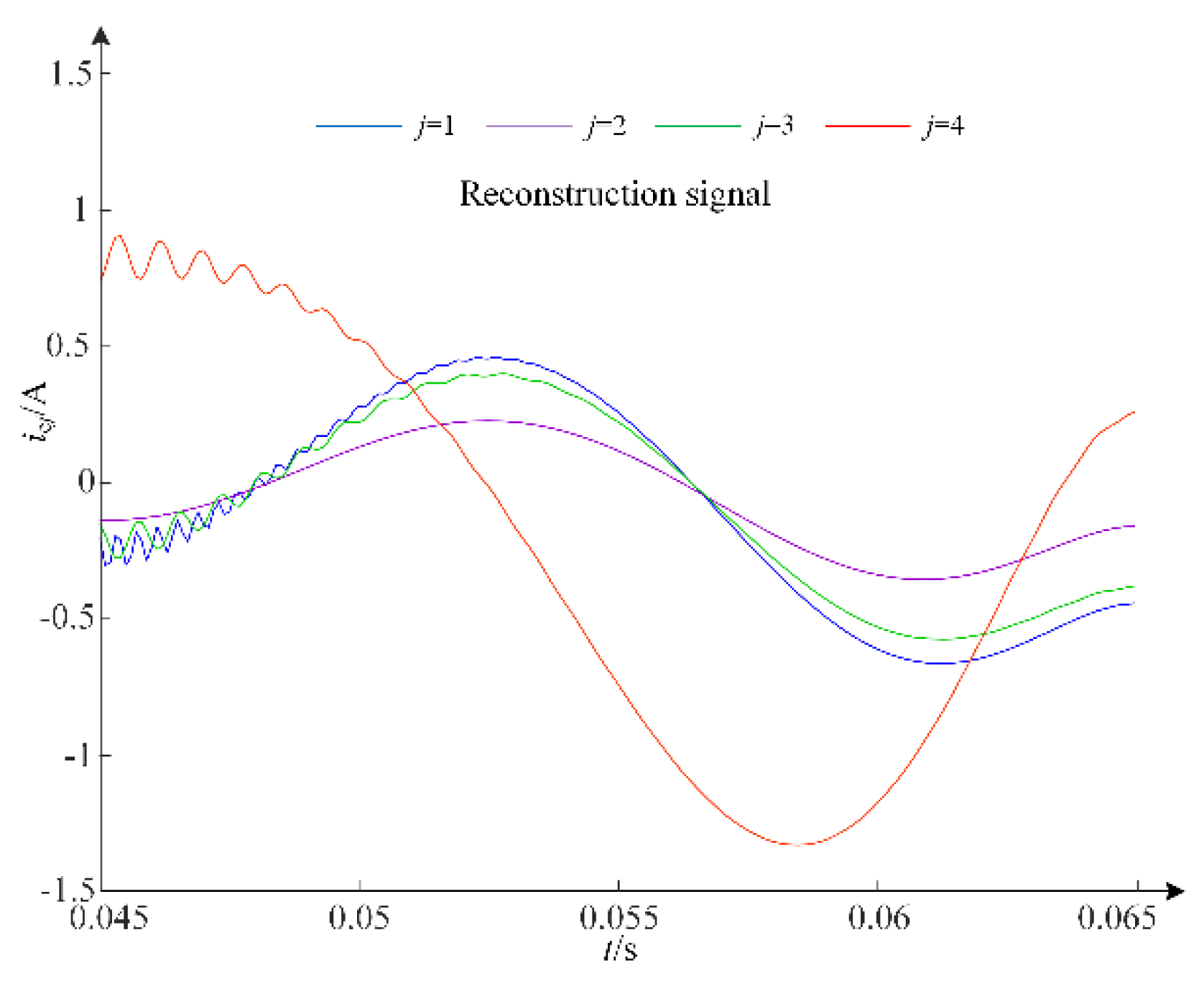
Figure 10.
Transient zero-sequence currents with the noise (SNR=5dB) and IMFs.
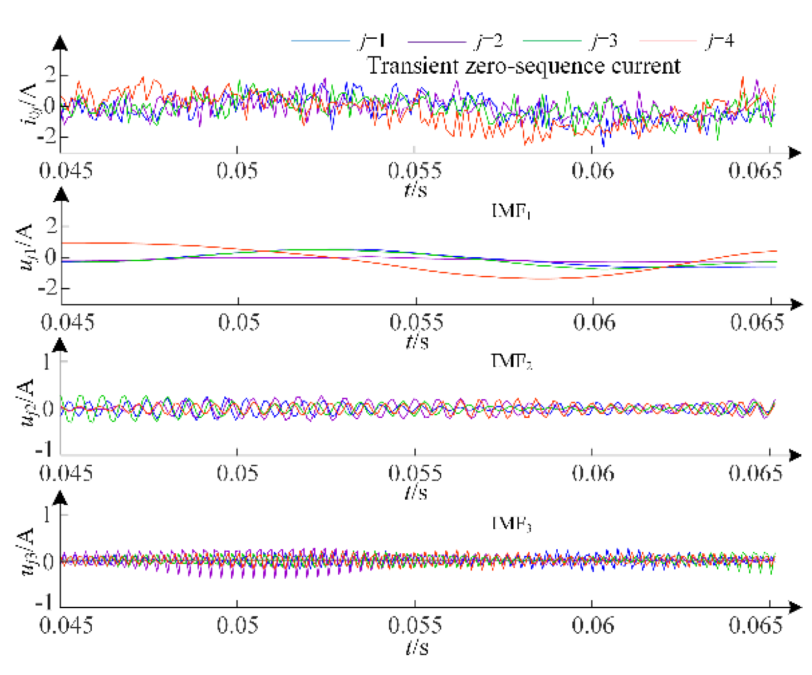
Figure 11.
High-frequency components of transient zero-sequence currents.
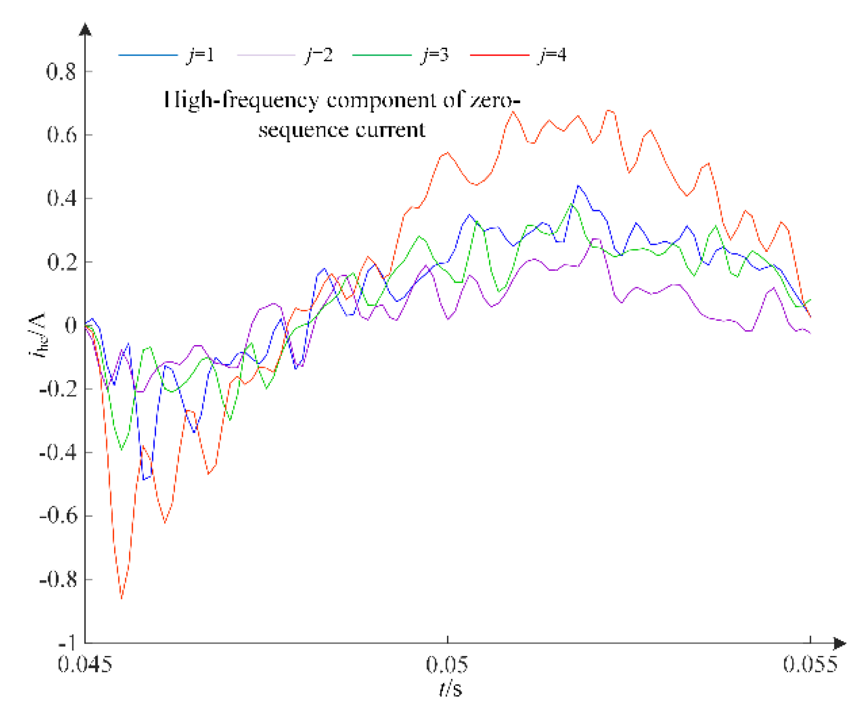
Figure 12.
Low-frequency IMF1 of transient zero-sequence currents.
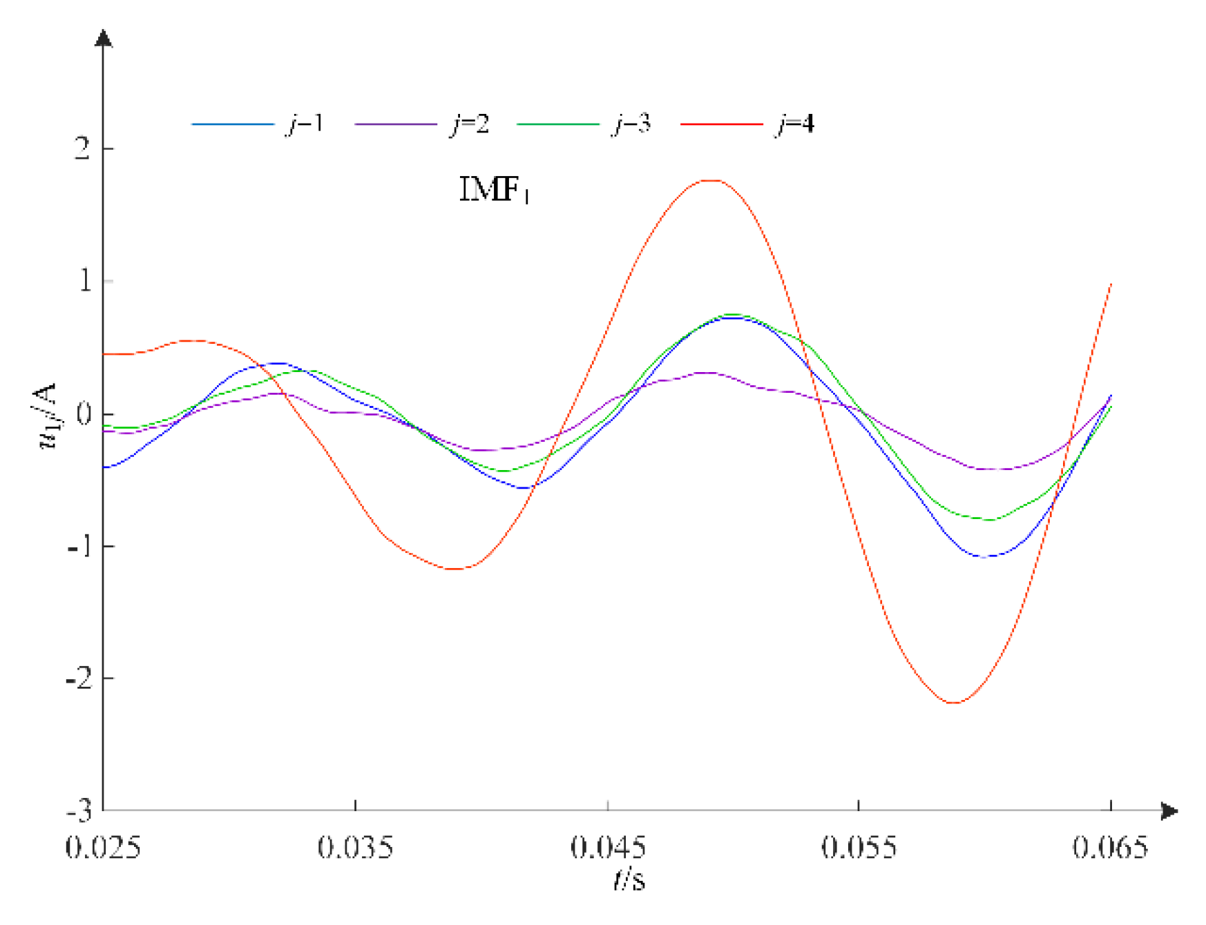
Figure 13.
Transient zero-sequence currents of field data and IMFs.
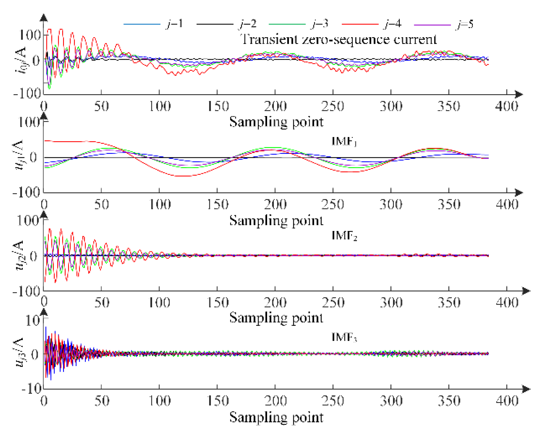
Figure 14.
Reconstruction signals of field data.
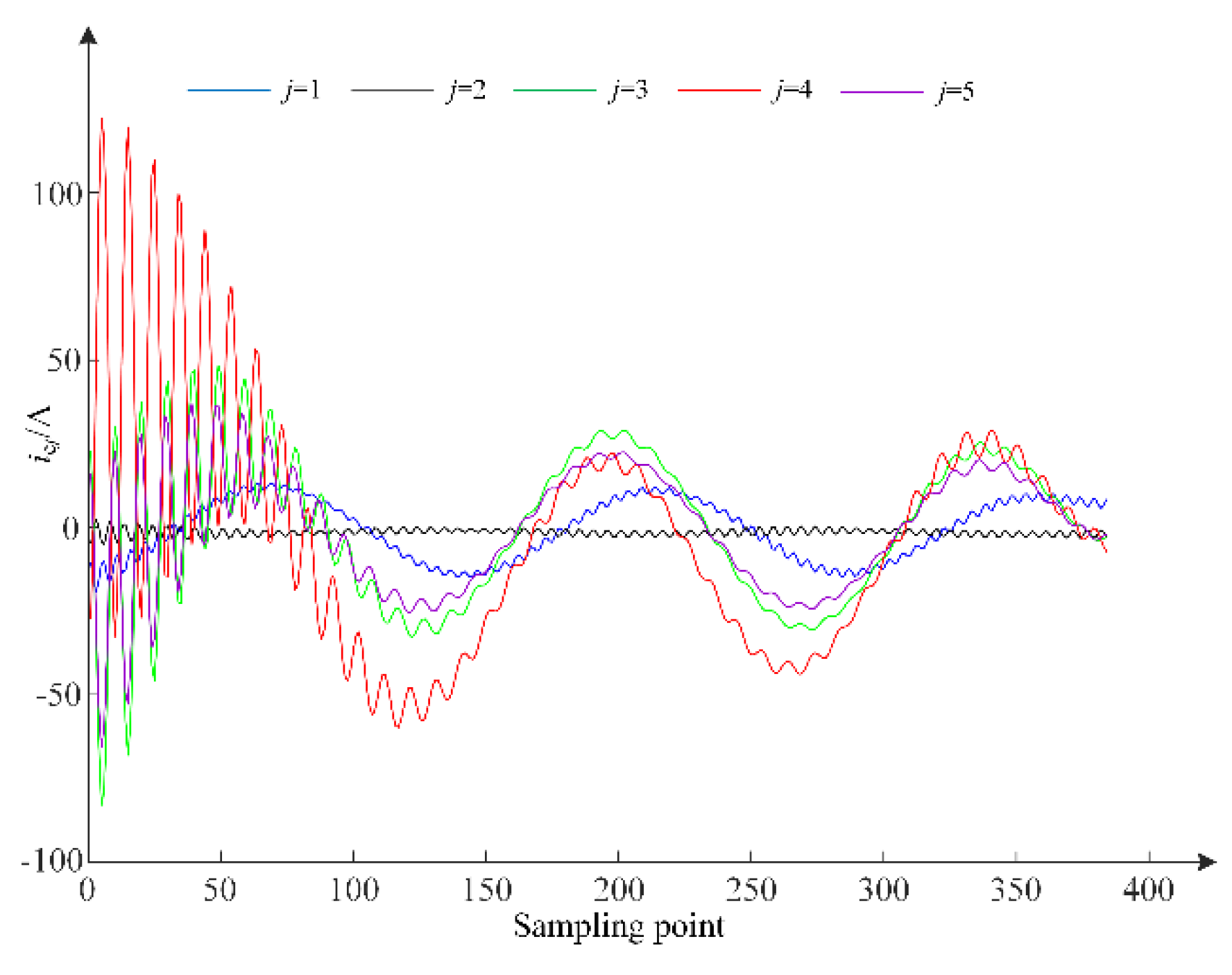

Table 1.
Feeder parameters.
| Line type | Phase-sequence |
R (Ω/km) |
L (mH/km) |
C (μF/km) |
|---|---|---|---|---|
| Overhead line | Phase-sequence | 0.125 | 1.3 | 0.0096 |
| Positive-sequence | 0.275 | 4.6 | 0.0054 | |
| Cable line | Zero-sequence | 0.27 | 0.255 | 0.339 |
| Positive-sequence | 2.7 | 1.019 | 0.28 |
Table 2.
Simulation results under various fault conditions.
| Cases | Fj | Position | φ(º) | Rg(Ω) | Ej | ρj | ηj | Results |
|---|---|---|---|---|---|---|---|---|
| 1 | 2 | 90% | 0 | 1 | 894, 22713, 673, 2051 | 0.9408, -0.9743, 0.9408 | 0.3294, -0.3412, 0.3294 | Feeder 2 |
| 2 | 2 | 90% | 45 | 1 | 1362, 29367, 1639, 5627 | -0.8768, 0.9439, 0.9439 | -0.3171, 0.3414, 0.3414 | Feeder 2 |
| 3 | 2 | 90% | 90 | 10 | 1907, 22984, 1492, 9812 | 0.9929, -0.9034, 0.9929 | 0.3437, -0.3127, 0.3437 | Feeder 2 |
| 4 | 2 | 90% | 90 | 1000 | 5.1162, 132.7223, 4.2172, 19.239 | 0.8466, -0.6390, 0.8466 | 0.3630, -0.2740, 0.3630 | Feeder 2 |
| 5 | 4 | 10% | 0 | 2000 | 1.3112, 0.2898, 0.9835, 16.9661 | 1, 1, -0.9688 | 0.3368, 0.3368, -0.3263 | Feeder 4 |
| 6 | 4 | 10% | 45 | 100 | 297, 62.1, 224.12, 5190.3 | 0.9756, 0.9756, -0.6334 | 0.3775, 0.3775, -0.2451 | Feeder 4 |
| 7 | 4 | 10% | 45 | 3000 | 0.8764, 0.2035, 0.6637, 20.3033 | 0.9915, 0.9915, -0.7338 | 0.3649, 0.3649, -0.2701 | Feeder 4 |
| 8 | 4 | 10% | 90 | 3000 | 0.6884, 0.1935, 0.5229, 12.9077 | 0.9659, 0.9659, -0.4179 | 0.4111, 0.4111, -0.1779 | Feeder 4 |
| 9 | Bus | ‒ | 45 | 10 | 1050.2, 166.5, 883.9, 4175.1 | 0.8968, 0.9260, 0.9260 | 0.3262, 0.3369, 0.3369 | bus |
| 10 | Bus | ‒ | 90 | 100 | 346, 67, 277, 1297.3 | 0.9659, 0.9770, 0.9770 | 0.3308, 0.3346, 0.33465 | bus |
Table 3.
Simulation results under noise interference.
| Cases | Fi | Position | φ(º) | Rg(Ω) | SNR | Ej | ηj | Results |
|---|---|---|---|---|---|---|---|---|
| 1 | 2 | 90% | 45 | 100 | 5 | 249.4, 6173.4, 197.3, 863.7 | 0.3553, -0.2894, 0.3553 | Feeder 2 |
| 2 | 2 | 90% | 45 | 100 | 10 | 248.5, 6223.3, 192, 885.2 | 0.3563, -0.2874, 0.3563 | Feeder 2 |
| 3 | 2 | 90% | 45 | 100 | 20 | 238.9, 6323.3, 190.2, 935.7 | 0.3544, -0.2911, 0.3544 | Feeder 2 |
| 4 | 4 | 10% | 90 | 2000 | 5 | 3.4377, 1.1145, 2.1192, 29.1335 | 0.2902, 0.2902, -0.4197 | Feeder 4 |
| 5 | 4 | 10% | 90 | 2000 | 10 | 1.9031, 0.4352, 1.4652, 25.1508 | 0.3927, 0.3927, -0.2146 | Feeder 4 |
| 6 | 4 | 10% | 90 | 2000 | 20 | 1.2807, 0.3594, 1.1829, 28.0953 | 0.4142, 0.4142, -0.1716 | Feeder 4 |
| 7 | Bus | ‒ | 0 | 10 | 5 | 544.2, 121.9, 408.1, 1997.4 | 0.3333, 0.3333, 0.3333 | Bus |
| 8 | Bus | ‒ | 0 | 10 | 10 | 542.5, 126.5, 407.7, 1970.5 | 0.3332, 0.3334, 0.3334 | Bus |
| 9 | Bus | ‒ | 0 | 10 | 20 | 545.5, 122.4, 414.5, 1955.6 | 0.3332, 0.3334, 0.3334 | Bus |
Table 4.
Comparison of the faulty feeder detection accuracy of the proposed method with existing methods.
Table 4.
Comparison of the faulty feeder detection accuracy of the proposed method with existing methods.
| Fault criterion | SNR | Accuracy |
|---|---|---|
| [1] | 20 | 71% |
| [1] | 10 | 57% |
| [1] | 5 | 43% |
| [18] | 20 | 86% |
| [18] | 10 | 71% |
| [18] | 5 | 57% |
| this paper | 20 | 100% |
| this paper | 10 | 100% |
| this paper | 5 | 100% |
Table 5.
Faulty feeder detection result of field data.
| Ej | ρj | ηj | Results |
|---|---|---|---|
| 3190 220 50610, 139180, 30440 | 0.9781 -0.6678, 0.9781 | 0.3727, -0.2545, 0.3727 | Feeder 4 |
Disclaimer/Publisher’s Note: The statements, opinions and data contained in all publications are solely those of the individual author(s) and contributor(s) and not of MDPI and/or the editor(s). MDPI and/or the editor(s) disclaim responsibility for any injury to people or property resulting from any ideas, methods, instructions or products referred to in the content. |
© 2026 by the authors. Licensee MDPI, Basel, Switzerland. This article is an open access article distributed under the terms and conditions of the Creative Commons Attribution (CC BY) license.
Copyright: This open access article is published under a Creative Commons CC BY 4.0 license, which permit the free download, distribution, and reuse, provided that the author and preprint are cited in any reuse.