

Submitted:
13 March 2026
Posted:
16 March 2026
You are already at the latest version
Abstract
Item response theory (IRT) models are widely used in the social sciences to analyze multivariate discrete data that include cognitive test items. In many applications, the performance of two groups is compared using IRT modeling. The assessment of differential item functioning (DIF) plays a central role in this context, as it evaluates whether specific items function differently across groups; that is, whether their item parameters differ between groups. DIF detection is commonly based on statistical inference using item fit statistics. The mean deviation (MD) and root mean square deviation (RMSD) statistics are two widely used item fit measures. However, in the literature and in empirical research, these statistics are typically treated only as effect size measures (i.e., point estimates), and formal statistical inference for them is largely lacking. To address this gap, this article proposes confidence interval (CI) estimation for the MD and RMSD statistics based on asymptotic theory and a computationally efficient parametric bootstrap method. A simulation study was conducted to evaluate the proposed CI estimation approaches and demonstrated their validity. Across both item fit statistics, for DIF and non-DIF items, and across all simulation conditions, the results indicate that CI estimation based on the parametric bootstrap using empirical percentiles performed best and outperformed both the parametric bootstrap with normal distribution-based CIs and the asymptotic theory-based approach. It is therefore recommended that CI estimation for MD and RMSD statistics be routinely reported in addition to point estimates in empirical research.
Keywords:
item response model
; differential item functioning
; item fit
; root mean square deviation
; mean deviation
1. Introduction
Item response theory (IRT) models [1,2,3] are multivariate statistical models for analyzing vectors of discrete random variables. IRT models are widely applied in the social sciences, particularly in educational large-scale assessment (LSA; [4,5]) studies in which cognitive tasks are administered to persons.
This article focuses on dichotomous (i.e., binary) random variables. Let denote a vector of I random variables for , commonly referred to as items or scored item responses. A unidimensional IRT model [6] is a parametric model for the probability distribution for given by
where denotes the density of the normal distribution with mean and standard deviation (SD) , collected in the distribution parameter for the unidimensional latent variable , often called the trait or ability variable. The vector contains the item parameters for the item response functions (IRFs) for . The IRF of the two-parameter logistic (2PL) model [7] is
where and are the item discrimination and difficulty parameters, respectively, and is the logistic function. For the 2PL model, the item parameter vector is .
For a sample of N individuals with independently and identically distributed observations from the distribution of the random variable , the model parameters of the IRT model in (1) can be consistently estimated using marginal maximum likelihood estimation (MML; [8,9,10]). Note that identification constraints are required when estimating item parameters and distribution parameters simultaneously [11].
In LSA applications of IRT models, such as programme for international student assessment (PISA; [12]), a parametric model is imposed for the IRFs in (1). These studies involve a large number of countries, and item parameters are generally assumed to be identical across countries, implying parameter invariance [13,14,15]. In practice, however, this assumption may be violated, as certain items can systematically favor or disadvantage specific countries. This phenomenon is referred to as differential item functioning (DIF; [16,17,18]).
In LSA applications of the IRT model, the imposed invariance of item parameters across countries implies that the assumed IRF represents a misspecification of the true IRT model (1) for a given country (or group). Under this misspecified IRT model, the multivariate random vector is represented as
where denotes the assumed IRF and represents the true IRF in the data-generating model for the group. The item parameters are denoted by , reflecting that they introduce a model misspecification. In LSA applications, it is generally assumed that replacing with results in only minimal distortion of the estimated distribution parameters .
The assessment of the adequacy of parametric IRFs (i.e., item fit; [19,20]) is a central topic in psychometrics. The discrepancy between the true IRF and the assumed parametric IRF should be quantified using an appropriate item fit statistic, which can also serve as an effect size measure relatively independent of sample size. Ideally, a clear definition of the corresponding population value of the item fit statistic for an infinite sample should exist. It is also desirable that statistical inference, such as the computation of confidence intervals (CI) for these effect sizes, be available. Of primary interest to applied researchers is the detection of misfitting items i, for which the assumed IRFs deviate substantially from .
A lot of item fit statistics has been proposed in the psychometric literature [20]. The present study targets on the root mean square deviation (RMSD; [21,22,23,24,25]) and the related mean deviation (MD) statistic. The motivation for a thorough investigation of these statistics lies in their operational use in current PISA studies.
The following two subsections outline the definition and estimation of the RMSD and MD item fit statistics.
1.1. RMSD Statistic
The RMSD statistic for item i defined at the population level is defined as (see [26,27])
where w denotes the estimated group density function, represents the true IRF, and denotes the assumed IRF in the IRT model. The RMSD statistic captures the weighted squared discrepancy between and , and equals 0 for an item that fits perfectly.
Typically, the integral in (4) is approximated using a grid of T points for of the variable [28], giving
where and . The distribution weights are assumed to be proportional to and sum to 1, i.e., .
Using the notation , , , and , the RMSD definition in (5) can be written compactly as
As the RMSD statistic in (6) contains the unknown group-specific IRF , the expression cannot be used directly for estimation. An estimate of the group-specific IRF is therefore required. This estimation relies on individual posterior distributions, which arise as a by-product of MML estimation in the IRT model (see [29,30]).
Let denote the estimated posterior probability for person n at grid point . It is computed as
Using this posterior distribution, an estimate for item response probabilities can be obtained by
Define . It follows that
Substituting with in (6) yields the sample RMSD statistic
It is important to emphasize that sampling variability in induces corresponding sampling variability in the estimated RMSD statistic . Because RMSD item fit statistics are used to identify potentially misfitting items, point estimates of the RMSD statistic should be supplemented with inferential tools such as standard errors, CIs, and tests assessing whether the population RMSD differs from 0 (but see [31]). However, the existing literature on this topic is extremely limited.
Finally, the sample-based RMSD statistic depends on sample size through its expected value, because
Note that this relies on the property that is an unbiased estimate of (see (9)). The second term in (11) introduces bias determined by the sampling variance of (see [32,33]). This bias in carries over to the RMSD estimate . As the sampling variance of approaches zero with increasing sample size, the sample-based statistic converges to the population value . Consequently, statistical inference for at a fixed sample size pertains to inference about the pseudo-true value , which exceeds . The pseudo-true RMSD value corresponds to the value of this statistic at a fixed sample size for a given dataset. Note that the proportion of misfitting items affects the pseudo-true value, which is larger for smaller sample sizes [32].
1.2. MD Statistic
In contrast to the RMSD statistic, the MD statistic is signed and may take positive or negative values. It is particularly informative for detecting uniform DIF, where the differences are uniformly positive or uniformly negative; such patterns are captured directly by . However, the MD statistic is less suited to identifying misfit in the functional form of IRFs.
Using the discrete grid of values, the MD statistic becomes
The corresponding sample-based version is
Using (9), it follows that
Hence, the expected value of the MD statistic is independent of sample size, which may be viewed as an advantage over the RMSD statistic.
1.3. Goal of this Paper
Although the RMSD and MD item fit statistics are widely used in LSA applications [12,23,34], methodological work on statistical inference for these statistics remains limited. In particular, the availability of CIs would be a valuable addition for identifying misfitting items. Preliminary developments have been presented in [32], but that work relies on a coarse approximation for quantifying uncertainty in the RMSD statistic. An alternative approach in the same study employs a nonparametric bootstrap [32], which is computationally intensive because it requires repeated estimation of the IRT scaling model for each bootstrap sample.
To address these limitations, the present article develops CI estimation procedures based on asymptotic theory and a less computationally demanding parametric bootstrap. The proposed methods are evaluated through a simulation study.
The remainder of the article is structured as follows. Section 2 outlines the estimation procedures for constructing CIs for the RMSD and MD item fit statistics. Section 3 presents a simulation study evaluating the performance of these CI estimators under various conditions. Finally, Section 4 and Section 5 present the discussion and the conclusion.
2. Confidence Intervals for RMSD and MD Statistics
In this section, CI estimation methods for the RMSD and MD item fit statistics are introduced based on asymptotic theory and parametric bootstrap.
The key observation is that the sampling variability of the sample-based RMSD and MD statistics arises from the sampling variability of the group-specific IRF estimates . Consequently, uncertainty quantification for these item fit statistics requires the variance matrix .
An estimate of can be obtained using M-estimation theory [35,36,37]. From (8), the estimates satisfy
Hence, the variance matrix follows from standard M-estimation arguments [35]. The explicit expressions for the entries of are as follows.
For the diagonal entries , it holds that
For the off-diagonal entries with , it holds that
M-estimation theory implies that the estimates are approximately multivariate normally distributed with mean vector and variance matrix .
The CI derivations in the next two subsections are based on the estimated variance matrix .
2.1. Confidence Intervals Based on Asymptotic Theory
CI estimates for the MD and RMSD statistics can now be derived using asymptotic theory. The derivation for the MD item fit statistic is presented first.
Using the definition of the sample-based MD statistic in (14), its variance is
The corresponding standard error is therefore
A 95% CI for is obtained as
A CI estimate for the sample-based RMSD statistic is now derived. Let the squared RMSD statistic be denoted as the mean square deviation (MSD). Because is a quadratic form of a multivariate normal vector, its distribution does not have a convenient closed-form expression [39]. However, its variance can be approximated as
A computable estimate is obtained by substituting with , giving
Since the RMSD statistic is the square root of the MSD statistic, applying the delta method [36] to yields (see [33])
The standard error of is therefore
A 95% CI for the sample-based RMSD statistic is given by
2.2. Confidence Intervals Based on Parametric Bootstrap
The distribution of the RMSD and MD statistics is approximated numerically via a parametric bootstrap. Note that the IRF estimates are approximately multivariate normally distributed with mean vector and variance matrix . Because the item fit statistics are functions of , the parametric bootstrap generates repeated draws from a multivariate normal distribution with mean and variance matrix and evaluates the statistics for each draw. The resulting empirical distribution of the computed values serves for uncertainty quantification and hypothesis testing (see also [40] for a related approach).
To this end, a vector is simulated from a multivariate normal distribution with zero mean and variance matrix . The bootstrap-based estimated IRF is then computed as
The RMSD statistic for a bootstrap replicate, denoted by , is defined as
The corresponding MD statistic based on bootstrap is
The principal advantage of the numerical bootstrap approach is that the resulting distributions of the RMSD and MD statistics are not required to follow a normal distribution. This article applies two alternative CI estimation procedures based on bootstrap.
First, a CI is constructed under a normality assumption, using the SD of the RMSD or MD estimates across bootstrap samples as the standard error in CI computation. Because the normality assumption may be inappropriate for the RMSD statistic, a bootstrap percentile CI is also employed, with the bounds of the 95% CI defined by the 2.5% and 97.5% empirical percentiles.
Although no substantial differences are expected between the CI estimation approaches for the parametric bootstrap applied to the linear MD statistic, meaningful differences may arise for the nonlinear RMSD statistic. These differences are anticipated because the RMSD statistic is more likely to violate the normality assumption.
3. Simulation Study
In this Simulation Study, the performance of alternative CI estimation methods for the RMSD and MD item fit statistics is examined.
3.1. Method
The 2PL model was used for data generaation and for the IRT scaling model. The mean and SD of the normally distributed factor variable were set to 0 and 1, respectively.
The simulation study utilized items to represent conditions involving sufficiently long tests, which facilitates DIF detection. Ten base items with fixed item discriminations and item difficulties were defined and then duplicated four times to form a test comprising 40 items. All item discriminations were fixed at 1. The item difficulties of the ten base items were set to −1.80, −1.40, −1.00, −0.60, −0.20, 0.20, 0.60, 1.00, 1.40, and 1.80. These ten base item parameters were subsequently duplicated four times.
In total, two of the 40 items were simulated to exhibit uniform DIF. Items j and for were specified to display uniform DIF in their difficulties with values and , respectively. The DIF effect size was set to and , representing large DIF magnitudes [18,27,41].
The sample sizes N were set to 125, 250, 500, 1000, 2000, and 4000, reflecting typical applications of item fit statistics in small-scale or large-scale assessment studies using the 2PL model [4,5,42].
In each of the 6 (sample size N) × 5 (selected DIF items) × 2 (DIF effect size ) simulation conditions, 3000 replications were conducted. Item parameters in the 2PL IRT scaling model were fixed at the parameters of the ten base items. However, the presence of DIF was ignored in the scaling step to allow DIF detection by the MD and RMSD item fit statistics. In the scaling step, only the mean and the SD were estimated, while the item parameters remained fixed. Based on the individual posterior distributions obtained in the scaling model, the MD and RMSD statistics were computed.
Means, SDs, and skewness were computed for the item fit statistics as descriptive summaries. CIs were obtained using asymptotic theory (ASY; see Section 2.1) and a parametric bootstrap for the residuals (see Section 2.2). The parametric bootstrap does not require drawing new person samples or re-estimating the scaling model; it only recomputes the fit statistics based on simulated residuals . Because the parametric bootstrap of residuals relies on repeated draws from a multivariate normal distribution, it is subject to Monte Carlo error, which decreases only with larger numbers of bootstrap samples.
As an alternative, quasi Monte Carlo methods based on a deterministic distribution that minimizes Monte Carlo error were used. Specifically, 1000 multidimensional data points covering a multidimensional uniform distribution with independent components were generated using a Sobol sequence [43], implemented by the function qrng::sobol() in R (Version 4.4.1; [44]) within the qrng package (Version 0.0-10; [45]). These vectors were transformed via the inverse standard normal distribution function to approximate a multivariate normal distribution. This approach enables a fully numerical evaluation of the distribution of the MD and RMSD statistics in the parametric bootstrap procedure.
CIs under the parametric bootstrap were computed using two approaches: assuming a normal distribution for the bootstrap samples (BNO) and using empirical percentiles (BPE). A confidence level of 95% was applied throughout this Simulation Study.
To evaluate the performance of the alternative CI estimation methods, we computed coverage rates, power rates and Type I error rates. The coverage rate was computed as the percentage rate of events in which the pseudo-true parameter of the MD or RMSD item fit statistic lies within the computed CI. A pseudo-true parameter was computed as the average estimate of the fit statistic in a corresponding simulation condition because it is known that the expected value of the RMSD statistic depends on sample size [32]. Coverage rates within the range of 91% and 98% are considered acceptable.
Moreover, the percentage of cases was computed in which the lower bound of the CI included the value 0.05 for RMSD, and in which the CI for MD included 0.05 or −0.05, serving as a test of minimum effect size or close fit [46]. An RMSD value of 0.05 has been shown to be an effective cutoff for detecting DIF [47]. An exact test of an RMSD value of 0 is not feasible with the BPE method because empirical percentiles are always greater than 0. In addition, testing exact model fit (i.e., a population fit statistic of 0) is of limited practical relevance. For DIF items, the resulting percentage represents the power for rejecting close fit. For non-DIF items, these percentages correspond to Type I error rates.
All analyses for this Simulation Study were conducted in R (Version 4.4.1; [44]) using the sirt::xxirt() function in the sirt package (Version 4.2-133; [48]) to fit the 2PL scaling model. Dedicated R functions were written for computing the RMSD and MD statistics and their associated CI estimation methods. Replication materials are available at https://osf.io/jdf38 (accessed on 12 December 2025).
3.2. Results
Figure 1 displays boxplots of the MD statistic for the third item under conditions with DIF and without DIF. The sample distributions were approximately symmetric, and variability decreased as sample size increased. Moreover, the average MD statistics were relatively independent of sample size.
Table 1 presents descriptive statistics, coverage rates, and power rates for the MD item fit statistic for DIF items as a function of item difficulty , DIF effect and sample size N. The mean of the MD statistic was independent of sample size, whereas the SD decreased as sample size increased. In addition, the MD statistic had smaller absolute values for extreme item difficulties and the largest absolute values for item difficulties near 0. The distribution of the MD statistic was approximately symmetric, as indicated by skewness values close to 0.
The coverage rates for the ASY, BNO, and BPE CI estimation methods were all close to the nominal 95% level, indicating satisfactory performance of the MD item fit statistic for DIF items. Power rates increased with larger sample sizes, and the three CI estimation methods exhibited very similar power characteristics.
Table 2 presents descriptive statistics, coverage rates, and Type I error rates for the MD item fit statistic for non-DIF items as a function of item difficulty and sample size N. The mean of the MD statistic was essentially zero across conditions, indicating that the statistic accurately reflected the absence of DIF. Coverage rates for the three CI estimation methods were also close to the nominal 95% level. The Type I error rates were effectively 0%, indicating that false detections of DIF were virtually absent when items did not exhibit DIF in the data-generating model.
Figure 2 displays boxplots of the RMSD statistic for the third item under conditions with and without DIF. The sample distributions showed slight skewness, particularly for smaller sample sizes. Moreover, the average RMSD was larger for smaller sample sizes and converged to a fixed value as the sample size increased.
Table 3 presents descriptive statistics, coverage rates, and power rates for the RMSD item fit statistic for DIF items as a function of item difficulty , DIF effect and sample size N. The mean of the RMSD statistic decreased with increasing sample size, indicating a small-sample bias. As with the MD statistic, the SD of the RMSD statistic decreased as sample size increased. The mean of the RMSD statistic was lower for items with extreme item difficulties. Moreover, notable skewness was observed in small samples, whereas the RMSD distribution for DIF items was approximately symmetric in large samples.
The coverage rates were acceptable for the CI based on asymptotic theory (ASY). In small samples, the percentile-based bootstrap CI (BPE) provided better coverage than the normal distribution-based bootstrap CI (BNO). However, in small samples, the power to detect DIF for items that exhibited DIF in the data-generating model was substantially higher for BPE compared to ASY and BNO.
Table 4 presents descriptive statistics, coverage rates, and Type I error rates for the RMSD item fit statistic for non-DIF items as a function of item difficulty and sample size N. As with the RMSD statistic for DIF items, the mean RMSD statistic decreased with increasing sample size. Substantial skewness was observed in the RMSD distribution, calling into question the validity of CI estimation methods that rely on normality assumptions.
Coverage rates were satisfactory for BPE, whereas inflated coverage was observed for the ASY and BNO methods, both of which depend on the normal distribution assumption. Type I error rates were close to 0, with the exception of BPE in the smallest sample size of .
4. Discussion
In this article, CI estimation methods for the MD and RMSD statistics were compared, including those based on asymptotic theory (ASY) and parametric bootstrap. The parametric bootstrap was computationally efficient because only the residuals directly used in the MD and RMSD statistics were resimulated, without requiring repeated estimation of the 2PL scaling model. Such repeated estimation would be substantially more demanding when using large numbers of bootstrap samples. The parametric bootstrap yielded empirical distributions of the resampled MD and RMSD statistics, enabling the computation of bootstrap CIs based on the normal distribution (BNO) and empirical percentiles (BPE).
Overall, the three CI estimation methods exhibited highly similar performance with respect to coverage rates, power rates, and Type I error rates for the MD item fit statistic. This result aligns with the observation that the MD statistic is approximately normally distributed, with no indication of skewness.
The situation differed when considering CI estimation for the RMSD item fit statistic. This statistic exhibited strongly skewed distributions, particularly in small sample sizes. As a consequence of this skewness, the ASY and BNO methods produced unacceptable coverage rates and lower power for rejecting a close fit of RMSD; that is, they were less effective in detecting cases where the sample RMSD was significantly larger than a population RMSD value of 0.05, a threshold indicating close fit and thus an item with no or only minor DIF (or misfit).
As with any simulation study, several limitations apply that might suggest directions for future research on constructing CIs for the MD and RMSD item fit statistics. First, only DIF in item difficulties was examined; DIF in item discriminations was not considered. It is expected that DIF in item discriminations is more difficult to detect with the RMSD statistic, and the MD statistic is generally less suitable for detecting misfitting items in this case. Second, the data-generating model was limited by the absence of variation in item discriminations; that is, all item discriminations were fixed at 1 in the simulation study. This setting is unrealistic in practical datasets but was chosen for convenience in order not to confound the effects of item difficulty on the performance of the fit statistics and their estimated CIs with item discriminations, since the performance of the procedures can be expected to depend on item discriminations. Third, DIF was the sole source of misfit under investigation, although misfit in the functional form of the item response function is also relevant. This situation differs from the assessment of item fit across groups. Misspecifications in the item response functions are frequently assessed within a single group, implying that the uncertainty in estimated item parameters, which also determines the expected item response functions in the RMSD and MD statistics, must be taken into account for CI estimation. M-estimation theory and the parametric bootstrap must be adapted in this case. Fourth, only dichotomous item responses were studied, despite the fact that real-world assessments often include polytomous responses. No conceptual differences are apparent for CI computation in the case of polytomous item responses. However, ambiguity remains regarding how the RMSD statistic can be extended from the dichotomous to the polytomous case.
In educational large-scale assessments, item response data frequently involved student sampling weights and clustered samples. The CI computation techniques presented in this paper relied on the variance matrix of empirical item response probabilities calculated using M-estimation theory (see Section 2). The variance easily accommodated sampling weights by multiplying the case-wise terms by these weights. Moreover, M-estimation theory also allowed variance estimation under stratified cluster sampling, which could be incorporated into the formulas. Alternatively, the required variance matrix for CI computation could be obtained using resampling techniques such as jackknife, balanced repeated replication, or the nonparametric bootstrap.
5. Conclusion
It has been shown that confidence intervals based on both asymptotic theory and the parametric bootstrap work well for the MD item fit statistic, which is approximately symmetric in samples. However, because the RMSD statistic has a skewed distribution, the parametric bootstrap with a percentile-based confidence interval outperforms the confidence interval based on asymptotic theory, which relies on the normal distribution.
Funding
No funding was received for this research.
Artificial Intelligence (AI) Tools Declaration
The authors confirm that no AI tools were used in the construction of this research.
Acknowledgments
We are very grateful to experts for their appropriate and constructive suggestions to improve this template.
Conflicts of Interest
The authors declare that they have no known competing financial interests or personal relationships that could have appeared to influence the work reported in this paper.
References
- Baker, F.B.; Kim, S.H. Item Response Theory: Parameter Estimation Techniques; CRC Press: Boca Raton, 2004. [Google Scholar] [CrossRef]
- Bock, R.D.; Gibbons, R.D. Item Response Theory; Wiley, 2021. [Google Scholar] [CrossRef]
- Chen, Y.; Li, X.; Liu, J.; Ying, Z. Item response theory – A statistical framework for educational and psychological measurement. Statistical Science 2025, 40, 167–194. [Google Scholar] [CrossRef]
- Lietz, P.; Cresswell, J.C.; Rust, K.F.; Adams, R.J. (Eds.) Implementation of Large-scale Education Assessments; Wiley: New York, 2017. [Google Scholar] [CrossRef]
- Rutkowski, L.; von Davier, M.; Rutkowski, D. (Eds.) A Handbook of International Large-scale Assessment: Background, Technical Issues, and Methods of Data Analysis; Chapman Hall/CRC Press: London, 2013. [Google Scholar] [CrossRef]
- van der Linden, W.J. Unidimensional logistic response models. In Handbook of Item Response Theory, Volume 1: Models; van der Linden, W.J., Ed.; CRC Press: Boca Raton, 2016; pp. 11–30. [Google Scholar] [CrossRef]
- Birnbaum, A. Some latent trait models and their use in inferring an examinee’s ability. In Statistical Theories of Mental Test Scores; Lord, F.M., Novick, M.R., Eds.; MIT Press: Reading, MA, 1968; pp. 397–479. [Google Scholar]
- Aitkin, M. Expectation maximization algorithm and extensions. In Handbook of Item Response Theory, Volume 2: Statistical Tools; van der Linden, W.J., Ed.; CRC Press: Boca Raton, 2016; pp. 217–236. [Google Scholar] [CrossRef]
- Bock, R.D.; Aitkin, M. Marginal maximum likelihood estimation of item parameters: Application of an EM algorithm. Psychometrika 1981, 46, 443–459. [Google Scholar] [CrossRef]
- Glas, C.A.W. Maximum-likelihood estimation. In Handbook of Item Response Theory, Volume 2: Statistical Tools; van der Linden, W.J., Ed.; CRC Press: Boca Raton, 2016; pp. 197–216. [Google Scholar] [CrossRef]
- San Martin, E. Identification of item response theory models. In Handbook of Item Response Theory, Volume 2: Statistical Tools; van der Linden, W.J., Ed.; CRC Press: Boca Raton, 2016; pp. 127–150. [Google Scholar] [CrossRef]
- OECD. PISA 2018. Technical Report; OECD: Paris, 2020; Available online: https://bit.ly/3zWbidA.
- Davidov, E.; Meuleman, B.; Cieciuch, J.; Schmidt, P.; Billiet, J. Measurement equivalence in cross-national research. Annual Review of Sociology 2014, 40, 55–75. [Google Scholar] [CrossRef]
- Leitgöb, H.; Seddig, D.; Asparouhov, T.; Behr, D.; Davidov, E.; De Roover, K.; Jak, S.; Meitinger, K.; Menold, N.; Muthén, B.; et al. Measurement invariance in the social sciences: Historical development, methodological challenges, state of the art, and future perspectives. Social Science Research 2023, 110, 102805. [Google Scholar] [CrossRef] [PubMed]
- Millsap, R.E. Statistical Approaches to Measurement Invariance; Routledge: New York, 2011. [Google Scholar] [CrossRef]
- Holland, P.W.; Wainer, H. (Eds.) Differential Item Functioning: Theory and Practice; Lawrence Erlbaum: Hillsdale, NJ, 1993. [Google Scholar] [CrossRef]
- Mellenbergh, G.J. Item bias and item response theory. International Journal of Educational Research 1989, 13, 127–143. [Google Scholar] [CrossRef]
- Penfield, R.D.; Camilli, G. Differential item functioning and item bias. In Handbook of Statistics, Vol. 26: Psychometrics; Rao, C.R., Sinharay, S., Eds.; 2007; pp. 125–167. [Google Scholar] [CrossRef]
- Sinharay, S.; Haberman, S.J. How often is the misfit of item response theory models practically significant? Educational Measurement: Issues and Practice 2014, 33, 23–35. [Google Scholar] [CrossRef]
- Swaminathan, H.; Hambleton, R.K.; Rogers, H.J. Assessing the fit of item response theory models. In Handbook of Statistics, Vol. 26: Psychometrics; Rao, C.R., Sinharay, S., Eds.; 2007; pp. 683–718. [Google Scholar] [CrossRef]
- Buchholz, J.; Hartig, J. Comparing attitudes across groups: An IRT-based item-fit statistic for the analysis of measurement invariance. Applied Psychological Measurement 2019, 43, 241–250. [Google Scholar] [CrossRef]
- Kunina-Habenicht, O.; Rupp, A.A.; Wilhelm, O. A practical illustration of multidimensional diagnostic skills profiling: Comparing results from confirmatory factor analysis and diagnostic classification models. Studies in Educational Evaluation 2009, 35, 64–70. [Google Scholar] [CrossRef]
- Joo, S.H.; Khorramdel, L.; Yamamoto, K.; Shin, H.J.; Robin, F. Evaluating item fit statistic thresholds in PISA: Analysis of cross-country comparability of cognitive items. Educational Measurement: Issues and Practice 2021, 40, 37–48. [Google Scholar] [CrossRef]
- Joo, S.; Ali, U.; Robin, F.; Shin, H.J. Impact of differential item functioning on group score reporting in the context of large-scale assessments. Large-scale Assessments in Education 2022, 10, 18. [Google Scholar] [CrossRef]
- von Davier, M.; Bezirhan, U. A robust method for detecting item misfit in large scale assessments. Educational Psychological Measurement 2023, 83, 740–765. [Google Scholar] [CrossRef] [PubMed]
- Joo, S.; Valdivia, M.; Svetina Valdivia, D.; Rutkowski, L. Alternatives to weighted item fit statistics for establishing measurement invariance in many groups. Journal of Educational and Behavioral Statistics 2024, 49, 465–493. [Google Scholar] [CrossRef]
- Robitzsch, A. Comparing weighted RMSD, weighted MD, infit, and outfit item fit statistics under uniform differential item functioning. Mathematics 2025, 13, 3752. [Google Scholar] [CrossRef]
- Köhler, C.; Robitzsch, A.; Hartig, J. A bias-corrected RMSD item fit statistic: An evaluation and comparison to alternatives. Journal of Educational and Behavioral Statistics 2020, 45, 251–273. [Google Scholar] [CrossRef]
- Sueiro, M.J.; Abad, F.J. Assessing goodness of fit in item response theory with nonparametric models: A comparison of posterior probabilities and kernel-smoothing approaches. Educational Psychological Measurement 2011, 71, 834–848. [Google Scholar] [CrossRef]
- Tijmstra, J.; Bolsinova, M.; Liaw, Y.L.; Rutkowski, L.; Rutkowski, D. Sensitivity of the RMSD for detecting item-level misfit in low-performing countries. Journal of Educational Measurement 2020, 57, 566–583. [Google Scholar] [CrossRef]
- Kim, Y.K.; Cai, L.; Kim, Y. Evaluation of item fit with output from the EM algorithm: RMSD index based on posterior expectations. Educational Psychological Measurement 2025. Epub ahead of print. [Google Scholar] [CrossRef] [PubMed]
- Robitzsch, A. Statistical properties of estimators of the RMSD item fit statistic. Foundations 2022, 2, 488–503. [Google Scholar] [CrossRef]
- Robitzsch, A. Bias-corrected root mean square deviation estimators. Foundations 2025, 5, 36. [Google Scholar] [CrossRef]
- Baghaei, P.; Robitzsch, A. A tutorial on item response modeling with multiple groups using TAM. Educational Methods & Psychometrics 2025, 3, 14. [Google Scholar] [CrossRef]
- Boos, D.D.; Stefanski, L.A. Essential Statistical Inference; Springer: New York, 2013. [Google Scholar] [CrossRef]
- Held, L.; Sabanés Bové, D. Applied Statistical Inference; Springer: Berlin, 2014. [Google Scholar] [CrossRef]
- Stefanski, L.A.; Boos, D.D. The calculus of M-estimation. The American Statistician 2002, 56, 29–38. [Google Scholar] [CrossRef]
- Kondratek, B. Item-fit statistic based on posterior probabilities of membership in ability groups. Applied Psychological Measurement 2022, 46, 462–478. [Google Scholar] [CrossRef] [PubMed]
- Rencher, A.C.; Schaalje, G.B. Linear Models in Statistics; Wiley: New York, 2008. [Google Scholar] [CrossRef]
- Chen, Y.; Li, C.; Ouyang, J.; Xu, G. DIF statistical inference without knowing anchoring items. Psychometrika 2023, 88, 1097–1122. [Google Scholar] [CrossRef] [PubMed]
- Zwick, R. A review of ETS differential item functioning assessment pocedures: Flagging rules, minimum sample size requirements, and criterion refinement (Research Report No. RR-12-08); Educational Testing Service: Princeton, NJ, 2012. [Google Scholar] [CrossRef]
- Yen, W.M.; Fitzpatrick, A.R. Item response theory. In Educational Measurement; Brennan, R.L., Ed.; Praeger Publishers: Westport, 2006; pp. 111–154. [Google Scholar]
- Jäckel, P. Monte Carlo Methods in Finance; Wiley: New York, 2002. [Google Scholar]
- R Core Team. R: A language and environment for statistical computing; Vienna, Austria, 2024; Available online: https://www.R-project.org (accessed on 15 June 2024).
- Hofert, M.; Lemieux, C. qrng: (Randomized) quasi-random number generators, 2024. R package version 0.0-10. Accessed on 29 February 2024. [CrossRef]
- Grissom, R.J.; Kim, J.J. Effect Sizes for Research: A Broad Practical Approach; Lawrence Erlbaum, 2005. [Google Scholar] [CrossRef]
- Robitzsch, A.; Lüdtke, O. A review of different scaling approaches under full invariance, partial invariance, and noninvariance for cross-sectional country comparisons in large-scale assessments. Psychological Test and Assessment Modeling 2020, 62, 233–279. Available online: https://bit.ly/3ezBB05.
- Robitzsch, A. sirt: Supplementary item response theory models, 2025. R package version 4.2-133. Accessed on 27 September 2025. [CrossRef]
Figure 1.
Simulation Study: Boxplots for the MD statistic for the third item (with item difficulty ) with DIF (left panel) and without DIF (right panel) as a function of sample size N
Figure 1.
Simulation Study: Boxplots for the MD statistic for the third item (with item difficulty ) with DIF (left panel) and without DIF (right panel) as a function of sample size N
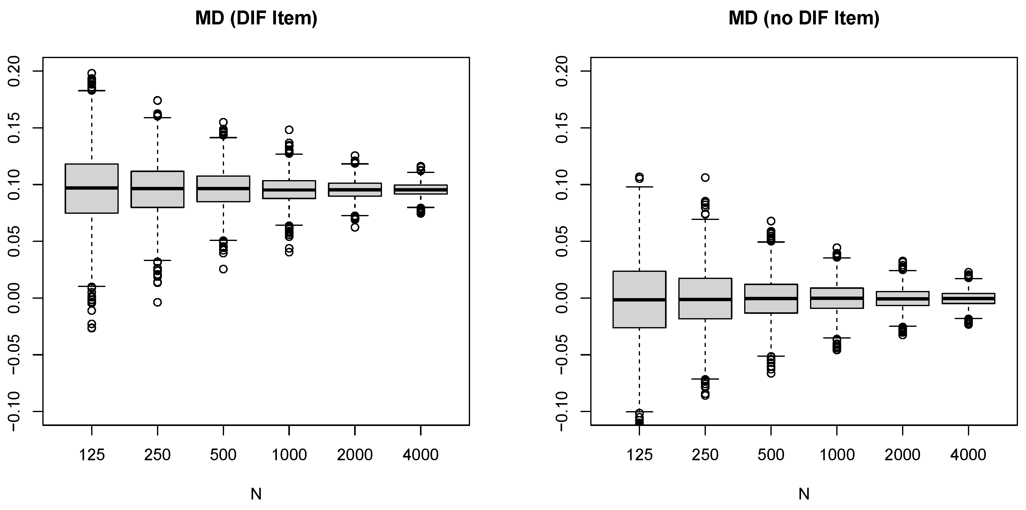
Figure 2.
Simulation Study: Boxplots for the RMSD statistic for the third item (with item difficulty ) with DIF (left panel) and without DIF (right panel) as a function of sample size N
Figure 2.
Simulation Study: Boxplots for the RMSD statistic for the third item (with item difficulty ) with DIF (left panel) and without DIF (right panel) as a function of sample size N
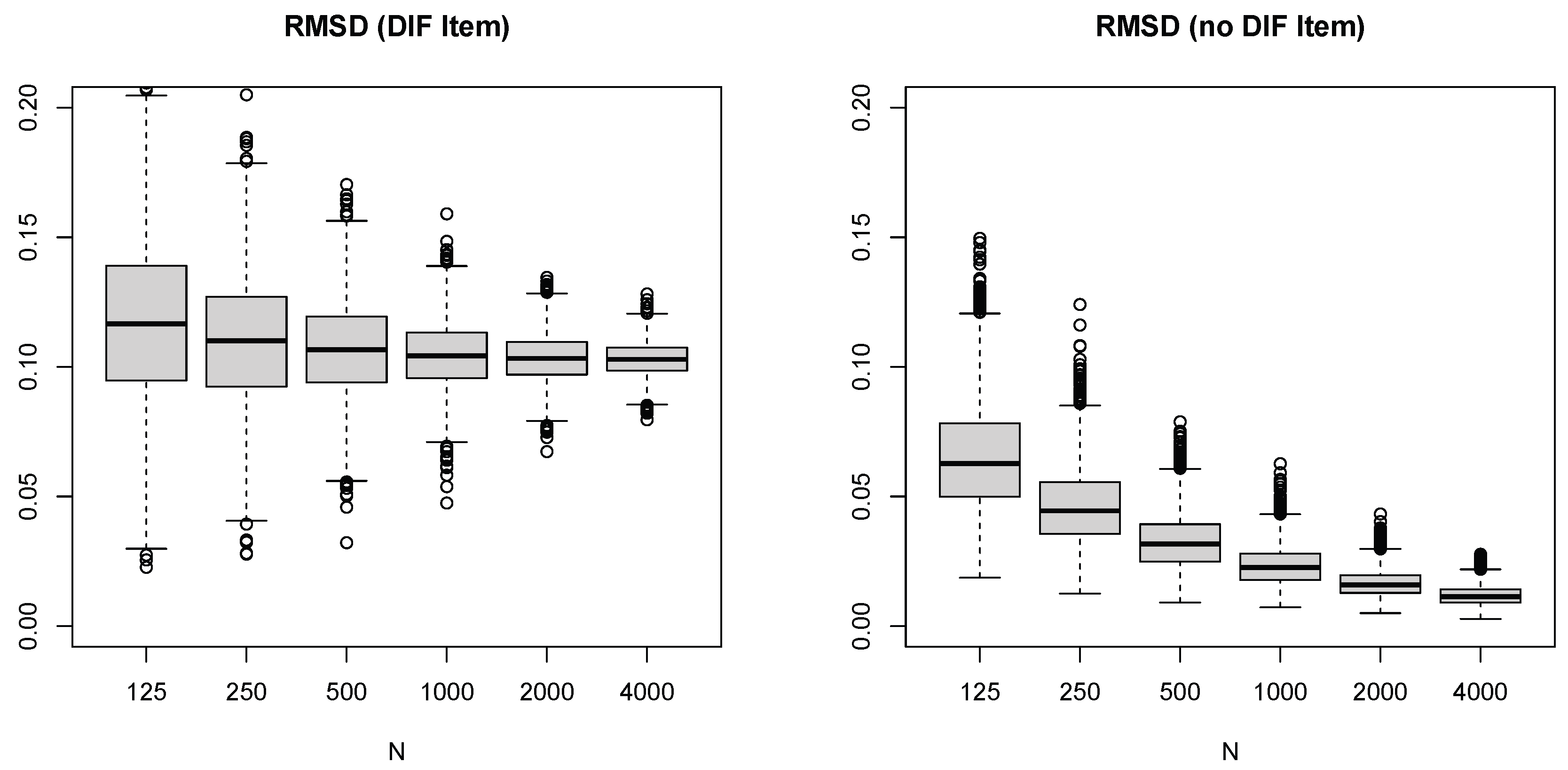

Table 1.
Simulation Study: Descriptive statistics, coverage rates and power rates for the MD statistic for DIF items as a function of item difficulty , DIF effect and sample size N
Table 1.
Simulation Study: Descriptive statistics, coverage rates and power rates for the MD statistic for DIF items as a function of item difficulty , DIF effect and sample size N
| Coverage rate | Power rate | ||||||||||
|---|---|---|---|---|---|---|---|---|---|---|---|
| M | SD | Skew | ASY | BNO | BPE | ASY | BNO | BPE | |||
| −1.8 | −0.6 | 125 | 0.065 | 0.027 | −0.156 | 92.9 | 92.9 | 92.9 | 13.4 | 13.3 | 13.4 |
| 250 | 0.065 | 0.019 | −0.080 | 93.8 | 93.8 | 93.7 | 14.6 | 14.5 | 14.7 | ||
| 500 | 0.065 | 0.013 | −0.025 | 94.8 | 94.8 | 94.7 | 21.6 | 21.6 | 21.9 | ||
| 1000 | 0.065 | 0.010 | −0.022 | 94.6 | 94.7 | 94.4 | 35.4 | 35.2 | 36.2 | ||
| 2000 | 0.065 | 0.007 | 0.032 | 95.0 | 95.0 | 94.6 | 57.9 | 57.7 | 59.1 | ||
| 4000 | 0.065 | 0.005 | −0.064 | 94.3 | 94.4 | 94.0 | 86.1 | 86.0 | 86.5 | ||
| 0.6 | 125 | −0.089 | 0.036 | −0.117 | 94.0 | 94.1 | 94.1 | 17.6 | 17.5 | 17.6 | |
| 250 | −0.088 | 0.026 | −0.107 | 93.9 | 94.0 | 93.9 | 31.7 | 31.6 | 31.7 | ||
| 500 | −0.088 | 0.018 | 0.025 | 94.3 | 94.4 | 94.2 | 56.6 | 56.4 | 56.9 | ||
| 1000 | −0.088 | 0.013 | −0.061 | 94.8 | 94.9 | 95.0 | 85.4 | 85.3 | 85.2 | ||
| 2000 | −0.088 | 0.009 | −0.029 | 95.0 | 95.1 | 94.7 | 98.8 | 98.8 | 98.9 | ||
| 4000 | −0.088 | 0.006 | −0.011 | 95.1 | 95.2 | 94.9 | 100.0 | 100.0 | 100.0 | ||
| −1.0 | −0.6 | 125 | 0.096 | 0.033 | −0.146 | 94.1 | 94.1 | 94.0 | 32.2 | 31.9 | 32.2 |
| 250 | 0.096 | 0.024 | −0.079 | 94.3 | 94.4 | 94.2 | 51.5 | 51.4 | 51.6 | ||
| 500 | 0.096 | 0.017 | −0.093 | 95.3 | 95.4 | 95.3 | 78.0 | 77.8 | 78.3 | ||
| 1000 | 0.096 | 0.012 | 0.010 | 94.8 | 94.8 | 94.7 | 97.0 | 97.0 | 97.1 | ||
| 2000 | 0.095 | 0.008 | 0.014 | 94.9 | 94.9 | 94.9 | 100.0 | 100.0 | 100.0 | ||
| 4000 | 0.096 | 0.006 | −0.021 | 95.1 | 95.1 | 95.2 | 100.0 | 100.0 | 100.0 | ||
| 0.6 | 125 | −0.113 | 0.040 | −0.021 | 94.3 | 94.4 | 94.2 | 36.6 | 36.5 | 37.1 | |
| 250 | −0.114 | 0.028 | −0.086 | 94.4 | 94.5 | 94.4 | 62.6 | 62.4 | 62.9 | ||
| 500 | −0.114 | 0.020 | −0.004 | 94.3 | 94.4 | 94.1 | 90.5 | 90.4 | 90.5 | ||
| 1000 | −0.114 | 0.014 | 0.026 | 94.8 | 94.9 | 94.7 | 99.5 | 99.5 | 99.5 | ||
| 2000 | −0.114 | 0.010 | −0.098 | 94.4 | 94.4 | 94.5 | 100.0 | 100.0 | 100.0 | ||
| 4000 | −0.114 | 0.007 | −0.014 | 95.6 | 95.7 | 95.5 | 100.0 | 100.0 | 100.0 | ||
| −0.2 | −0.6 | 125 | 0.118 | 0.038 | −0.041 | 94.1 | 94.1 | 94.1 | 44.4 | 44.1 | 44.3 |
| 250 | 0.119 | 0.027 | −0.078 | 95.1 | 95.1 | 95.1 | 72.1 | 71.9 | 72.5 | ||
| 500 | 0.119 | 0.019 | 0.012 | 95.2 | 95.1 | 95.1 | 94.7 | 94.6 | 95.0 | ||
| 1000 | 0.119 | 0.013 | −0.048 | 95.2 | 95.4 | 94.8 | 99.9 | 99.9 | 99.9 | ||
| 2000 | 0.119 | 0.010 | −0.029 | 95.1 | 95.2 | 95.0 | 100.0 | 100.0 | 100.0 | ||
| 4000 | 0.119 | 0.007 | −0.056 | 95.1 | 95.2 | 95.1 | 100.0 | 100.0 | 100.0 | ||
| 0.6 | 125 | −0.124 | 0.040 | 0.077 | 94.4 | 94.4 | 94.3 | 47.5 | 47.4 | 48.2 | |
| 250 | −0.124 | 0.028 | 0.031 | 94.4 | 94.4 | 94.5 | 75.3 | 75.3 | 75.7 | ||
| 500 | −0.124 | 0.020 | 0.030 | 94.8 | 94.8 | 94.7 | 96.6 | 96.6 | 96.6 | ||
| 1000 | −0.123 | 0.015 | 0.041 | 93.9 | 93.9 | 93.9 | 99.8 | 99.8 | 99.8 | ||
| 2000 | −0.124 | 0.010 | 0.027 | 94.9 | 94.9 | 94.9 | 100.0 | 100.0 | 100.0 | ||
| 4000 | −0.123 | 0.007 | −0.004 | 95.2 | 95.2 | 95.1 | 100.0 | 100.0 | 100.0 | ||
Note. M = mean; SD = standard deviation; Skew = skewness; CI = confidence interval; ASY = CI based on asymptotic theory; BNO = CI based on normal distribution; BPE = CI based on empirical percentiles; Coverage rates smaller than 91.0 or larger than 98.0 are printed in bold font. Power rates smaller than 80.0 are printed in bold font.
Table 2.
Simulation Study: Descriptive statistics, coverage rates and power rates for the MD statistic for non-DIF items as a function of item difficulty and sample size N
Table 2.
Simulation Study: Descriptive statistics, coverage rates and power rates for the MD statistic for non-DIF items as a function of item difficulty and sample size N
| Coverage rate | Type I error rate | |||||||||
|---|---|---|---|---|---|---|---|---|---|---|
| M | SD | Skew | ASY | BNO | BPE | ASY | BNO | BPE | ||
| −1.8 | 125 | 0.000 | 0.032 | −0.138 | 93.8 | 93.8 | 93.7 | 0.0 | 0.0 | 0.0 |
| 250 | 0.001 | 0.023 | −0.108 | 93.4 | 93.4 | 93.2 | 0.0 | 0.0 | 0.0 | |
| 500 | 0.000 | 0.016 | −0.071 | 95.2 | 95.2 | 95.1 | 0.0 | 0.0 | 0.0 | |
| 1000 | 0.000 | 0.011 | −0.105 | 95.3 | 95.3 | 95.2 | 0.0 | 0.0 | 0.0 | |
| 2000 | 0.001 | 0.008 | −0.031 | 95.6 | 95.7 | 95.5 | 0.0 | 0.0 | 0.0 | |
| 4000 | 0.001 | 0.006 | −0.013 | 94.4 | 94.4 | 94.5 | 0.0 | 0.0 | 0.0 | |
| −1.4 | 125 | 0.000 | 0.035 | −0.073 | 94.4 | 94.4 | 94.5 | 0.1 | 0.1 | 0.1 |
| 250 | 0.001 | 0.025 | −0.101 | 94.1 | 94.2 | 94.2 | 0.0 | 0.0 | 0.0 | |
| 500 | 0.000 | 0.017 | 0.011 | 94.8 | 94.8 | 94.9 | 0.0 | 0.0 | 0.0 | |
| 1000 | 0.001 | 0.012 | −0.103 | 94.8 | 94.9 | 94.6 | 0.0 | 0.0 | 0.0 | |
| 2000 | 0.001 | 0.009 | −0.065 | 95.0 | 95.0 | 94.8 | 0.0 | 0.0 | 0.0 | |
| 4000 | 0.001 | 0.006 | 0.025 | 96.2 | 96.2 | 95.9 | 0.0 | 0.0 | 0.0 | |
| −0.6 | 125 | 0.001 | 0.040 | −0.087 | 94.2 | 94.2 | 94.1 | 0.2 | 0.2 | 0.2 |
| 250 | 0.001 | 0.027 | −0.028 | 95.4 | 95.4 | 95.3 | 0.0 | 0.0 | 0.0 | |
| 500 | 0.000 | 0.019 | 0.012 | 95.3 | 95.4 | 95.4 | 0.0 | 0.0 | 0.0 | |
| 1000 | 0.001 | 0.014 | 0.004 | 95.2 | 95.2 | 95.1 | 0.0 | 0.0 | 0.0 | |
| 2000 | 0.000 | 0.010 | 0.053 | 94.5 | 94.6 | 94.2 | 0.0 | 0.0 | 0.0 | |
| 4000 | 0.000 | 0.007 | −0.030 | 94.5 | 94.5 | 94.2 | 0.0 | 0.0 | 0.0 | |
| −0.2 | 125 | −0.001 | 0.040 | −0.018 | 94.8 | 94.8 | 94.6 | 0.1 | 0.1 | 0.1 |
| 250 | 0.000 | 0.028 | 0.036 | 94.9 | 94.9 | 94.8 | 0.0 | 0.0 | 0.0 | |
| 500 | 0.000 | 0.020 | −0.088 | 94.6 | 94.6 | 94.3 | 0.0 | 0.0 | 0.0 | |
| 1000 | 0.000 | 0.014 | 0.014 | 94.6 | 94.7 | 94.7 | 0.0 | 0.0 | 0.0 | |
| 2000 | 0.000 | 0.010 | −0.049 | 95.5 | 95.5 | 95.2 | 0.0 | 0.0 | 0.0 | |
| 4000 | 0.000 | 0.007 | 0.065 | 94.3 | 94.3 | 94.1 | 0.0 | 0.0 | 0.0 | |
Note. M = mean; SD = standard deviation; Skew = skewness; CI = confidence interval; ASY = CI based on asymptotic theory; BNO = CI based on normal distribution; BPE = CI based on empirical percentiles; Coverage rates smaller than 91.0 or larger than 98.0 are printed in bold font. Type I error rates larger than 5.0 are printed in bold font.
Table 3.
Simulation Study: Descriptive statistics, coverage rates and power rates for the RMSD statistic for DIF items as a function of item difficulty , DIF effect and sample size N
Table 3.
Simulation Study: Descriptive statistics, coverage rates and power rates for the RMSD statistic for DIF items as a function of item difficulty , DIF effect and sample size N
| Coverage rate | Power rate | ||||||||||
|---|---|---|---|---|---|---|---|---|---|---|---|
| M | SD | Skew | ASY | BNO | BPE | ASY | BNO | BPE | |||
| −1.8 | −0.6 | 125 | 0.090 | 0.028 | 0.267 | 91.3 | 89.8 | 90.7 | 31.4 | 34.6 | 63.3 |
| 250 | 0.082 | 0.022 | 0.222 | 92.8 | 90.8 | 93.2 | 31.5 | 35.0 | 54.1 | ||
| 500 | 0.079 | 0.016 | 0.057 | 93.9 | 92.8 | 93.6 | 42.4 | 44.3 | 58.9 | ||
| 1000 | 0.077 | 0.012 | 0.036 | 94.3 | 93.7 | 94.2 | 62.4 | 63.6 | 72.9 | ||
| 2000 | 0.075 | 0.008 | 0.070 | 95.0 | 94.9 | 94.5 | 85.0 | 85.7 | 90.1 | ||
| 4000 | 0.075 | 0.006 | −0.049 | 94.5 | 94.4 | 94.0 | 98.2 | 98.3 | 98.9 | ||
| 0.6 | 125 | 0.114 | 0.035 | 0.277 | 94.2 | 90.5 | 95.3 | 38.6 | 45.3 | 77.0 | |
| 250 | 0.105 | 0.027 | 0.198 | 94.4 | 92.1 | 94.6 | 50.3 | 55.8 | 75.1 | ||
| 500 | 0.100 | 0.020 | −0.009 | 94.4 | 93.3 | 94.5 | 74.0 | 75.9 | 84.6 | ||
| 1000 | 0.098 | 0.014 | 0.064 | 95.1 | 94.7 | 95.2 | 93.0 | 93.7 | 96.5 | ||
| 2000 | 0.097 | 0.010 | 0.028 | 94.8 | 94.7 | 94.8 | 99.9 | 99.9 | 99.9 | ||
| 4000 | 0.096 | 0.007 | 0.027 | 95.4 | 95.3 | 95.2 | 100.0 | 100.0 | 100.0 | ||
| −1.0 | −0.6 | 125 | 0.117 | 0.033 | 0.122 | 93.1 | 90.5 | 94.1 | 51.6 | 57.4 | 85.1 |
| 250 | 0.110 | 0.025 | 0.046 | 94.3 | 92.6 | 93.7 | 66.6 | 70.2 | 85.2 | ||
| 500 | 0.107 | 0.018 | −0.037 | 95.5 | 94.5 | 95.1 | 86.2 | 87.7 | 94.3 | ||
| 1000 | 0.104 | 0.013 | 0.044 | 95.1 | 94.7 | 94.5 | 98.5 | 98.7 | 99.5 | ||
| 2000 | 0.103 | 0.009 | 0.034 | 94.8 | 94.7 | 94.8 | 100.0 | 100.0 | 100.0 | ||
| 4000 | 0.103 | 0.007 | 0.008 | 95.1 | 95.2 | 95.0 | 100.0 | 100.0 | 100.0 | ||
| 0.6 | 125 | 0.132 | 0.037 | 0.202 | 94.3 | 91.2 | 94.2 | 56.4 | 63.2 | 90.1 | |
| 250 | 0.126 | 0.028 | 0.121 | 94.8 | 92.7 | 93.8 | 77.4 | 81.3 | 92.7 | ||
| 500 | 0.122 | 0.021 | −0.016 | 94.6 | 94.1 | 94.3 | 94.9 | 95.9 | 98.1 | ||
| 1000 | 0.120 | 0.015 | −0.037 | 94.8 | 94.6 | 94.7 | 99.9 | 100.0 | 100.0 | ||
| 2000 | 0.119 | 0.010 | 0.105 | 94.6 | 94.4 | 94.7 | 100.0 | 100.0 | 100.0 | ||
| 4000 | 0.119 | 0.007 | 0.020 | 95.7 | 95.6 | 95.4 | 100.0 | 100.0 | 100.0 | ||
| −0.2 | −0.6 | 125 | 0.136 | 0.036 | 0.137 | 94.5 | 91.7 | 93.9 | 61.8 | 69.0 | 92.4 |
| 250 | 0.129 | 0.027 | 0.020 | 95.2 | 93.7 | 94.6 | 82.5 | 85.8 | 95.3 | ||
| 500 | 0.126 | 0.019 | 0.018 | 95.5 | 95.2 | 95.3 | 97.6 | 98.1 | 99.2 | ||
| 1000 | 0.124 | 0.014 | −0.030 | 95.2 | 94.9 | 94.9 | 100.0 | 100.0 | 100.0 | ||
| 2000 | 0.123 | 0.010 | −0.023 | 94.9 | 94.8 | 94.7 | 100.0 | 100.0 | 100.0 | ||
| 4000 | 0.123 | 0.007 | −0.054 | 95.5 | 95.5 | 95.3 | 100.0 | 100.0 | 100.0 | ||
| 0.6 | 125 | 0.141 | 0.037 | 0.119 | 94.6 | 92.0 | 94.1 | 66.8 | 72.3 | 94.1 | |
| 250 | 0.133 | 0.028 | 0.059 | 94.2 | 92.7 | 94.4 | 85.6 | 88.3 | 95.7 | ||
| 500 | 0.130 | 0.020 | 0.001 | 95.1 | 94.5 | 94.8 | 98.0 | 98.6 | 99.5 | ||
| 1000 | 0.128 | 0.015 | −0.018 | 94.4 | 94.1 | 94.0 | 99.9 | 99.9 | 100.0 | ||
| 2000 | 0.128 | 0.010 | −0.033 | 94.9 | 94.8 | 94.9 | 100.0 | 100.0 | 100.0 | ||
| 4000 | 0.127 | 0.007 | −0.009 | 95.1 | 95.1 | 95.1 | 100.0 | 100.0 | 100.0 | ||
Note. M = mean; SD = standard deviation; Skew = skewness; CI = confidence interval; ASY = CI based on asymptotic theory; BNO = CI based on normal distribution; BPE = CI based on empirical percentiles; Coverage rates smaller than 91.0 or larger than 98.0 are printed in bold font. Power rates smaller than 80.0 are printed in bold font.
Table 4.
Simulation Study: Descriptive statistics, coverage rates and power rates for the RMSD statistic for non-DIF items as a function of item difficulty and sample size N
Table 4.
Simulation Study: Descriptive statistics, coverage rates and power rates for the RMSD statistic for non-DIF items as a function of item difficulty and sample size N
| Coverage rate | Type I error rate | |||||||||
|---|---|---|---|---|---|---|---|---|---|---|
| M | SD | Skew | ASY | BNO | BPE | ASY | BNO | BPE | ||
| −1.8 | 125 | 0.060 | 0.020 | 0.575 | 98.0 | 98.5 | 92.8 | 2.5 | 3.2 | 20.9 |
| 250 | 0.043 | 0.015 | 0.649 | 98.5 | 98.9 | 93.6 | 0.3 | 0.4 | 2.2 | |
| 500 | 0.031 | 0.010 | 0.699 | 98.7 | 98.9 | 94.3 | 0.0 | 0.0 | 0.1 | |
| 1000 | 0.022 | 0.007 | 0.773 | 99.0 | 98.8 | 94.9 | 0.0 | 0.0 | 0.0 | |
| 2000 | 0.015 | 0.005 | 0.625 | 99.2 | 99.3 | 94.9 | 0.0 | 0.0 | 0.0 | |
| 4000 | 0.011 | 0.004 | 0.741 | 98.9 | 99.0 | 95.0 | 0.0 | 0.0 | 0.0 | |
| −1.4 | 125 | 0.063 | 0.021 | 0.641 | 98.5 | 98.7 | 93.1 | 2.7 | 3.4 | 26.4 |
| 250 | 0.046 | 0.015 | 0.689 | 98.7 | 98.9 | 94.0 | 0.3 | 0.3 | 2.9 | |
| 500 | 0.032 | 0.011 | 0.710 | 98.9 | 99.1 | 94.0 | 0.0 | 0.0 | 0.1 | |
| 1000 | 0.023 | 0.007 | 0.697 | 99.1 | 99.1 | 94.8 | 0.0 | 0.0 | 0.0 | |
| 2000 | 0.016 | 0.005 | 0.676 | 99.2 | 99.1 | 94.7 | 0.0 | 0.0 | 0.0 | |
| 4000 | 0.011 | 0.004 | 0.638 | 99.0 | 99.2 | 94.8 | 0.0 | 0.0 | 0.0 | |
| −0.6 | 125 | 0.068 | 0.023 | 0.636 | 98.2 | 98.4 | 94.1 | 3.2 | 4.1 | 37.1 |
| 250 | 0.048 | 0.015 | 0.662 | 99.2 | 99.1 | 94.9 | 0.3 | 0.4 | 3.6 | |
| 500 | 0.034 | 0.011 | 0.659 | 98.8 | 99.1 | 94.2 | 0.0 | 0.0 | 0.2 | |
| 1000 | 0.024 | 0.008 | 0.643 | 99.1 | 98.9 | 94.2 | 0.0 | 0.0 | 0.0 | |
| 2000 | 0.017 | 0.005 | 0.654 | 99.2 | 98.9 | 94.2 | 0.0 | 0.0 | 0.0 | |
| 4000 | 0.012 | 0.004 | 0.577 | 99.1 | 98.8 | 94.4 | 0.0 | 0.0 | 0.0 | |
| −0.2 | 125 | 0.068 | 0.022 | 0.616 | 99.0 | 99.1 | 93.7 | 2.7 | 4.0 | 37.0 |
| 250 | 0.048 | 0.015 | 0.632 | 99.3 | 99.1 | 94.6 | 0.3 | 0.4 | 4.0 | |
| 500 | 0.034 | 0.011 | 0.665 | 99.0 | 99.0 | 94.2 | 0.0 | 0.0 | 0.1 | |
| 1000 | 0.024 | 0.008 | 0.629 | 99.2 | 98.9 | 94.5 | 0.0 | 0.0 | 0.0 | |
| 2000 | 0.017 | 0.005 | 0.598 | 99.3 | 99.2 | 94.5 | 0.0 | 0.0 | 0.0 | |
| 4000 | 0.012 | 0.004 | 0.646 | 99.3 | 99.0 | 94.1 | 0.0 | 0.0 | 0.0 | |
Note. M = mean; SD = standard deviation; Skew = skewness; CI = confidence interval; ASY = CI based on asymptotic theory; BNO = CI based on normal distribution; BPE = CI based on empirical percentiles; Coverage rates smaller than 91.0 or larger than 98.0 are printed in bold font. Type I error rates larger than 5.0 are printed in bold font.
Disclaimer/Publisher’s Note: The statements, opinions and data contained in all publications are solely those of the individual author(s) and contributor(s) and not of MDPI and/or the editor(s). MDPI and/or the editor(s) disclaim responsibility for any injury to people or property resulting from any ideas, methods, instructions or products referred to in the content. |
© 2026 by the authors. Licensee MDPI, Basel, Switzerland. This article is an open access article distributed under the terms and conditions of the Creative Commons Attribution (CC BY) license (http://creativecommons.org/licenses/by/4.0/).
Copyright: This open access article is published under a Creative Commons CC BY 4.0 license, which permit the free download, distribution, and reuse, provided that the author and preprint are cited in any reuse.