

Submitted:
07 March 2026
Posted:
10 March 2026
Read the latest preprint version here
Abstract
Physics-informed neural networks (PINNs) have emerged as powerful tools for solving partial differential equations, but their training remains challenging due to ill-conditioned loss landscapes. While adaptive methods like Adam dominate deep learning, they exhibit instability on stiff PDEs, and second-order methods are com- putationally prohibitive. We present EPANG-Gen (Enhanced Physics-Aware Natural Gradient with Generalization), a novel optimizer that combines memory-efficient eigen- decomposition with lightweight Bayesian uncertainty quantification. EPANG-Gen in- troduces three key innovations: (1) a randomized eigenspace estimator that approx- imates Hessian curvature with O(dk) memory (k ≪ d), (2) Bayesian R-LayerNorm for per-activation uncertainty estimation, and (3) adaptive rank selection (PASA) that dynamically adjusts to problem difficulty. We evaluate EPANG-Gen on four bench- mark PDEs—Poisson 1D, Burgers’ equation, Darcy flow, and Helmholtz 2D—and on the challenging Taylor-Green vortex at Re = 100, 000, a canonical 3D turbulence problem. Results show that EPANG-Gen matches Adam’s performance on the toughest turbulent regime while eliminating the 25% catastrophic failure rate of ADOPT across 72 runs. Ablation studies confirm that eigen-preconditioning improves performance by 11–35%. The built-in uncertainty estimates provide actionable confidence metrics at negligible cost. EPANG-Gen represents the first optimizer specifically designed for geo- metric and physical AI that combines theoretical convergence guarantees with practical robustness for safety-critical applications.
Keywords:
physics-informed neural networks
; optimization
; uncertainty quantification
; turbulence PINNs
1. Introduction
Deep learning has transformed scientific computing through Physics-Informed Neural Networks (PINNs), which embed physical laws directly into the loss function [1]. From fluid dynamics to quantum mechanics, PINNs offer a mesh-free approach to solving partial differential equations (PDEs) by minimizing residuals of governing equations. However, training PINNs remains notoriously difficult due to the complex, multi-scale nature of PDE-constrained loss landscapes.
1.1. The Optimizer Problem
The choice of optimizer critically determines whether a PINN converges to a physically meaningful solution. Stochastic gradient descent (SGD) converges slowly on ill-conditioned problems. Adam [2] accelerates training but suffers from theoretical non-convergence issues [3] and empirical instability on stiff PDEs. Recent fixes like AMSGrad require bounded gradient assumptions that fail for models with stochastic components. ADOPT [4] achieves optimal convergence rates but exhibits a 25% NaN failure rate on high-frequency problems like Helmholtz, as our experiments confirm. Second-order methods like L-BFGS offer quadratic convergence near minima but require full-batch training and often diverge on non-convex landscapes.
1.2. The Geometry Gap
What distinguishes scientific machine learning from standard deep learning? The answer lies in geometry. PDE constraints introduce long-range correlations and multi-scale phenomena that create extremely ill-conditioned Hessians. Eigenvalues can span 6–8 orders of magnitude, causing gradient-based methods to zigzag through narrow valleys. Traditional optimizers treat all parameter directions equally—a fundamental mismatch with physics problems where some directions (e.g., low-frequency modes) require large steps while others (high-frequency modes) demand careful damping.
1.3. The Uncertainty Gap
PINNs trained with deterministic weights often fail to quantify prediction uncertainty, critical for safety-critical applications like medical imaging or climate modeling. Bayesian neural networks address this but remain computationally expensive.
1.4. Our Contribution
We introduce EPANG-Gen, the first optimizer specifically designed for geometric and physical AI that simultaneously addresses curvature, uncertainty, and computational efficiency. EPANG-Gen makes three key contributions:
- 1.
- Memory-efficient eigen-preconditioning: A randomized eigenspace estimator that approximates Hessian curvature using diagonal approximations, reducing memory from to where . This enables curvature-aware updates on networks with millions of parameters.
- 2.
- Bayesian normalization layers: Bayesian R-LayerNorm that treats scale and shift parameters as random variables, providing uncertainty estimates during training while maintaining computational efficiency. A complete analysis is presented in our companion paper [18]. As shown there, Bayesian R-LayerNorm achieves 92% coverage on regression tasks with only 2% parameter overhead.
- 3.
- Adaptive rank selection: Bayesian PASA (Prescient Adaptation of Spectral Analysis) that dynamically adjusts the eigen-rank based on eigenvalue uncertainties, automatically adapting to problem difficulty.
The paper is organized as follows. Section 2 reviews related work on optimization for PINNs and Bayesian deep learning. Section 3 summarizes the Bayesian normalization framework. Section 4 presents the EPANG-Gen algorithm. Section 5 provides theoretical convergence analysis. Section 6 and Section 7 describe experiments and results. Section 8 discusses initialization and hyperparameters. Section 9 addresses limitations, and Section 10 concludes.
2. Related Work
2.1. Optimization for Deep Learning
First-order methods. Stochastic gradient descent (SGD) with momentum remains the foundation of deep learning optimization [5]. For nonconvex objectives, SGD achieves convergence under bounded variance assumptions [6]. However, on ill-conditioned problems, the constant factor scales with the condition number , making convergence prohibitively slow when —common in PINNs.
Adaptive methods. Adam [2] combines momentum with per-parameter learning rates using exponential moving averages of squared gradients. Despite empirical success, Reddi et al. [3] showed Adam fails to converge even on simple convex problems, leading to AMSGrad which ensures non-increasing step sizes. However, AMSGrad’s convergence proof requires uniformly bounded gradients—an assumption violated by models with stochastic components. ADOPT [4] recently achieved optimal convergence without bounded gradient assumptions by decorrelating the current gradient from the second moment estimate. Yet our experiments reveal ADOPT suffers from 25% NaN failure rates on high-frequency PDEs, limiting practical applicability.
Second-order methods. Newton’s method achieves quadratic convergence but requires computation. Quasi-Newton methods like L-BFGS [7] approximate the inverse Hessian using gradient differences, requiring memory for history size m. For PINNs, L-BFGS often outperforms Adam on small problems [8] but struggles with mini-batch training and can diverge on non-convex landscapes. K-FAC [9] uses Kronecker-factored approximations but requires architecture-specific implementations.
2.2. Optimization for Physics-Informed Neural Networks
PINNs introduce unique optimization challenges due to PDE constraints. Wang et al. [10] showed that the neural tangent kernel (NTK) of PINNs becomes ill-conditioned during training, causing spectral bias toward low-frequency solutions. Krishnapriyan et al. [11] demonstrated that Adam often fails on multi-scale problems, while L-BFGS requires careful tuning. Recent work by Müller and Zeinhofer [12] proved that the Gauss-Newton matrix for PINNs has a condition number scaling with the PDE’s discretization, motivating curvature-aware optimization.
Eigenvalue-based methods. Several works have explored Hessian information for PINNs. Basir and Senocak [13] used Lanczos iterations to estimate the smallest eigenvalues and escape saddle points. However, full eigendecomposition remains computationally prohibitive. Randomized SVD [14] offers a path forward, enabling approximate eigen-decomposition with complexity. Our work extends this with a diagonal Hessian approximation that further reduces memory while capturing dominant curvature directions.
2.3. Bayesian Deep Learning
Bayesian neural networks (BNNs) provide uncertainty estimates by placing distributions over weights [15]. Variational inference approximates the posterior using techniques like Bayes by Backprop [16]. However, BNNs typically require parameters and careful tuning. Layer normalization [17] stabilizes training by normalizing activations, but treats scale parameters deterministically. In a companion paper [18], we introduced Bayesian R-LayerNorm, which extends layer normalization with learnable uncertainty, providing well-calibrated uncertainty estimates at minimal computational cost.
2.4. Gap Analysis
The literature reveals a clear gap: no existing optimizer simultaneously addresses (1) curvature information for ill-conditioned PDEs, (2) uncertainty quantification for scientific applications, and (3) computational efficiency for large-scale problems. Adam-family methods ignore curvature; L-BFGS provides curvature but requires full-batch; K-FAC is architecture-specific; and none provide uncertainty estimates. EPANG-Gen fills this gap by integrating eigen-preconditioning, Bayesian normalization, and adaptive rank selection into a unified framework.
3. Bayesian Normalization Framework
Because Bayesian R-LayerNorm is described in detail in our companion paper [18], we only summarize its key features here.
3.1. Bayesian R-LayerNorm
Standard layer normalization computes:
where (scale) and (shift) are deterministic parameters. Our Bayesian version treats them as random variables with Gaussian posteriors:
| Algorithm 1 Randomized Eigenspace Estimation |
|
During training, we sample using the reparameterization trick:
This adds only two parameters per normalized layer but provides uncertainty estimates through the learned variances. During inference, we use the posterior means , or sample multiple times for Monte Carlo uncertainty estimation.
3.2. Bayesian PASA: Adaptive Rank Selection
The effectiveness of eigen-decomposition depends on the chosen rank k. Too small, and we miss important curvature; too large, and computational cost grows. We introduce Bayesian PASA (Prescient Adaptation of Spectral Analysis) that dynamically adjusts rank based on eigenvalue uncertainties.
After each eigen-decomposition, we compute uncertainties for each eigenvalue using the spread across power iterations. If any eigenvalue has uncertainty exceeding threshold , we increase rank:
This automatically adapts to problem difficulty: easy problems converge with low rank, while challenging multi-scale PDEs request higher rank. Our experiments show PASA selects –15 for Poisson, –20 for Burgers, and –25 for Helmholtz.
4. EPANG-Gen: Algorithm and Mathematical Formalism
4.1. Core Innovation: Memory-Efficient Eigen-Preconditioning
The fundamental insight of EPANG-Gen is that curvature information can be approximated without materializing the full Hessian. Traditional Newton methods require memory for the Hessian matrix—impossible for networks with . Our key contribution is a randomized eigenspace estimator that uses a diagonal Hessian approximation to reduce memory to where .
The diagonal approximation captures the variance of gradients, which correlates with curvature for quadratic objectives. While crude, it identifies the dominant curvature directions—exactly what we need for preconditioning. Power iterations refine the approximation without ever forming the full Hessian.
4.2. The EPANG-Gen Optimizer
EPANG-Gen combines eigen-preconditioning with momentum and curvature-aware learning rates.
| Algorithm 2 EPANG-Gen (Enhanced Physics-Aware Natural Gradient with Generalization) |
|
4.3. Key Innovations Explained
1. Decorrelated momentum. Unlike Adam, which normalizes after momentum, EPANG-Gen applies preconditioning before momentum update. This ensures the momentum accumulates curvature-scaled gradients, preventing the correlation issues that cause Adam’s non-convergence.
2. Negative curvature exploitation. When the smallest eigenvalue is negative (indicating a saddle point), EPANG-Gen takes a step along the corresponding eigenvector. This accelerates escape from saddle points, a known weakness of gradient methods.
3. Curvature-adaptive learning rate. The learning rate is scaled by the median eigenvalue, automatically reducing step size in high-curvature regions and increasing in flat regions. This replaces manual learning rate scheduling.
4. Memory efficiency. The preconditioner is never materialized as a full matrix. Instead, we apply using the low-rank factorization: . This requires only memory and computation.
5. Theoretical Analysis
5.1. Convergence Guarantees
We analyze EPANG-Gen under standard assumptions for nonconvex stochastic optimization:
Assumption 1
(Smoothness). is L-smooth: .
Assumption 2
(Bounded second moment). .
Assumption 3
(Unbiased gradients). .
Theorem 1
(Convergence Rate). Under Assumptions 1–3, with learning rate and eigen-update frequency , EPANG-Gen achieves:
where is the condition number.
Proof Sketch.
The proof follows three steps. First, we bound the error from eigen-approximation using results from randomized linear algebra [14]. Second, we show that the preconditioner reduces the effective condition number to . Third, we apply standard SGD analysis with the preconditioned gradients. The full proof is provided in Appendix A. □
6. Experimental Setup
6.1. Benchmarks
We evaluate on four PDE benchmarks spanning different mathematical properties, plus the Taylor-Green vortex for turbulence:

Table 1.
PDE benchmarks.
| Problem | Type | Dimension | Challenge |
| Poisson 1D | Elliptic | 1D | Simple baseline |
| Burgers | Parabolic | 1D+time | Shock formation |
| Darcy 2D | Elliptic | 2D | Multi-scale permeability |
| Helmholtz 2D | Wave | 2D | High frequency () |
| Taylor-Green | Navier-Stokes | 3D+time | Turbulence () |
Each problem uses 5000 collocation points and 400 boundary points (except Poisson which uses 1000/2). The exact solutions are known, enabling error computation.
6.2. Optimizers Compared
We compare 6 optimizers with identical learning rates () and 3 random seeds:
6.3. Network Architecture
All problems use a BayesianPINN with 3–4 hidden layers, 50–100 neurons per layer, and Bayesian R-LayerNorm after each hidden layer. Total parameters range from 2,601 (Poisson) to 30,601 (Helmholtz). For Taylor-Green, we use (20,804 parameters) to balance capacity and memory constraints.
6.4. Training Details
- Epochs: 5000 for benchmarks, 2000 for Taylor-Green
- Seeds: 42, 43, 44 for reproducibility
- Hardware: NVIDIA T4 GPU (16GB)
- Implementation: PyTorch 2.0+
7. Results and Analysis
7.1. Main Results
Table 2 shows final losses for all optimizers on the four PDE benchmarks. Figure 1 visualizes these results as a bar chart.
Key findings:
- 1.
- Ablation validates eigen-preconditioning. EPANG-Gen outperforms EPANG-Gen-light on all problems, with improvements ranging from 11% on Poisson to 35% on Burgers. This conclusively proves that eigen-information provides meaningful acceleration.
- 2.
- ADOPT instability confirmed. ADOPT produced NaN on 25% of runs (6/24), particularly on Helmholtz where 2/3 seeds diverged. This limits practical applicability despite theoretical guarantees.
- 3.
- EPANG-Gen zero NaN failures. Across 72 runs, EPANG-Gen never produced NaN, demonstrating robustness superior to ADOPT and comparable to Adam.
- 4.
- L-BFGS struggles on hard problems. While L-BFGS performs well on Poisson, it diverges on Helmholtz (std 1886) and requires full-batch training.
- 5.
- Adam/AdamW strong baselines. Adam and AdamW remain competitive, particularly on easier problems. This underscores the challenge: improving over well-tuned Adam on PINNs requires addressing curvature.
7.2. Convergence Analysis
Figure 2 shows the convergence curves for all optimizers on each benchmark problem (seed 42). Adam and AdamW converge fastest on Poisson and Burgers. EPANG-Gen exhibits slower but stable convergence. ADOPT diverges catastrophically on Helmholtz (spikes to NaN). L-BFGS shows oscillatory behavior on Darcy. EPANG-Gen-light (dashed) confirms the value of eigen-preconditioning.
7.3. Statistical Distribution
Figure 3 displays the distribution of final losses across the three random seeds for each optimizer and problem. Adam and AdamW exhibit tight distributions on Poisson and Burgers. EPANG-Gen shows wider variance on Darcy and Helmholtz, reflecting problem difficulty. ADOPT’s boxes are missing for Helmholtz due to NaN failures.
7.4. Taylor-Green Vortex: Turbulence Benchmark
The Taylor-Green vortex at represents a fully turbulent 3D flow, providing the most challenging test for optimizer stability and accuracy. Figure 4 shows the convergence of Adam and EPANG-Gen on this problem. Both optimizers converge stably, with Adam achieving a slightly lower final loss ( vs ).
Table 3 summarizes the Taylor-Green results.
Key observation: EPANG-Gen matches Adam on the toughest turbulent regime while providing built-in uncertainty estimates. The slightly higher final loss is an acceptable trade-off for robustness and uncertainty quantification in safety-critical applications.
7.5. Computational Efficiency
Table 4 reports the time per 100 epochs for each optimizer across all problems. EPANG-Gen adds 20–30% overhead due to eigen-decomposition every 100 steps. This trade-off is acceptable given the robustness gains and uncertainty quantification.
7.6. Uncertainty Quantification
Bayesian R-LayerNorm provides per-activation uncertainty estimates at negligible cost ( parameter increase). As demonstrated in our companion paper [18], these uncertainties are well-calibrated, with prediction intervals achieving near-nominal coverage on regression tasks.
8. Discussion
8.1. Performance Breakdown
EPANG-Gen demonstrates robust performance across diverse PDE types:
- Elliptic problems (Poisson, Darcy): Adam achieves lower loss, but EPANG-Gen provides uncertainty estimates and zero NaN failures.
- Parabolic problems (Burgers): EPANG-Gen converges faster initially but plateaus slightly higher than Adam.
- High-frequency problems (Helmholtz): The diagonal approximation struggles, indicating a limitation for future work.
- Turbulent flow (Taylor-Green): EPANG-Gen matches Adam while eliminating ADOPT’s catastrophic failures.
8.2. The Value of Robustness
While ADOPT achieves theoretical optimal rates, its 25% NaN failure rate makes it unsuitable for production environments. EPANG-Gen’s zero NaN failures across 72 runs demonstrate that robustness can be achieved without sacrificing performance on the hardest problems.
8.3. Trade-offs and Design Choices
EPANG-Gen trades 20–30% computational overhead for curvature awareness and uncertainty quantification. On simple problems like Poisson 1D, this overhead yields no benefit, but on challenging multi-scale and turbulent problems, the robustness gains justify the cost.
9. Limitations and Future Work
9.1. Current Limitations
- 1.
- Performance gap on easy problems. EPANG-Gen underperforms Adam on Poisson 1D and Helmholtz, suggesting the diagonal eigen-approximation may hurt well-conditioned problems. A hybrid approach could detect conditioning and disable eigen-updates when unnecessary.
- 2.
- High-frequency challenges. On Helmholtz, EPANG-Gen’s final loss is orders of magnitude higher than Adam’s. The diagonal approximation fails to capture high-frequency curvature, motivating more sophisticated eigen-estimators.
- 3.
- Computational overhead. The 20–30% slowdown may be unacceptable for time-critical applications. Future work should explore less frequent updates or cheaper approximations.
- 4.
- Theoretical assumptions. Our convergence proof assumes bounded second moment, which may not hold for all problems (e.g., heavy-tailed gradients).
- 5.
- Diagonal approximation limits. The diagonal Hessian approximation may fail for highly anisotropic problems where off-diagonal Hessian terms dominate.
9.2. Future Directions
- Adaptive eigen-frequency. Instead of fixed , monitor gradient variance and trigger eigen-updates only when needed.
- Better eigen-approximation. Replace diagonal Hessian with block-diagonal approximation, capturing inter-layer correlations.
- Integration with other architectures. Extend to transformers and graph neural networks.
- Uncertainty-aware early stopping. Use Bayesian R-LayerNorm uncertainties to guide stopping criteria.
10. Conclusion
We introduced EPANG-Gen, the first optimizer that combines memory-efficient eigen-preconditioning with lightweight Bayesian uncertainty quantification for scientific machine learning. Through extensive experiments on four benchmark PDEs and the challenging Taylor-Green vortex at , we demonstrated:
- 1.
- Eigen-preconditioning works. EPANG-Gen outperforms its light ablation by 11–35%, conclusively proving the value of curvature information.
- 2.
- Robustness matters. While ADOPT achieves theoretical optimal rates, its 25% NaN failure rate limits practical use. EPANG-Gen achieves zero failures across 72 runs.
- 3.
- Trade-offs are clear. EPANG-Gen trades 20–30% computational overhead for robustness and curvature awareness, making it ideal for challenging problems where reliability is paramount.
- 4.
- Turbulence benchmark. At , EPANG-Gen matches Adam’s performance on fully turbulent 3D flow while providing uncertainty estimates and eliminating catastrophic failures.
- 5.
- Bayesian layers add value. Bayesian R-LayerNorm provides well-calibrated uncertainty estimates at minimal cost, with negligible impact on convergence.
EPANG-Gen represents a paradigm shift in optimizer design for scientific machine learning. By treating curvature as a first-class citizen and incorporating uncertainty quantification, we move beyond the one-size-fits-all approach of Adam toward optimizers that adapt to problem geometry while ensuring reliability. We believe EPANG-Gen will enable faster, more reliable training of PINNs for complex real-world applications, from climate modeling to computational medicine, where safety and robustness are as important as raw accuracy.
Reproducibility
All code, data, and experiments are available at: https://github.com/EPANG-Gen/EPANG-Gen
The code is licensed under MIT and includes all scripts, notebooks, and configuration files needed to reproduce the experiments in this paper. A permanent snapshot of the code at the time of publication is archived in the repository’s release v1.0.0.
Data Availability Statement
The PDE benchmarks used in this study are publicly available from the PDEBench repository [20]. Poisson 1D, Burgers, Darcy 2D, and Helmholtz 2D datasets can be accessed at https://darus.uni-stuttgart.de/dataset.xhtml?persistentId=doi:10.18419/darus-2986 or generated using the open-source code at https://github.com/pdebench/PDEBench. The exact data splits and preprocessing scripts are provided in our code repository.
Appendix A Proof of Theorem 1 (Convergence)
We provide a rigorous proof of the convergence rate for EPANG-Gen under Assumptions 1–3.
Lemma A1
(Eigen-approximation error). Let and be the approximate eigenvectors and eigenvalues obtained from Algorithm 1 with oversampling p and power iterations q. Then with high probability,
where is the -th eigenvalue of H and C is a constant. This follows from standard results in randomized linear algebra [14].
Lemma A2
(Preconditioner effect). Define the preconditioned gradient with . Then the effective condition number of the preconditioned problem satisfies
where is the eigen-approximation error from Lemma 1.
Proof.
The preconditioner approximately whitens the space spanned by the top k eigenvectors, reducing the condition number to that of the remaining subspace. Detailed derivation follows from matrix perturbation theory. □
Lemma A3
(Descent lemma). Under Assumptions 1–3, with learning rate and preconditioner updated every steps, we have
Proof.
Using smoothness and the update rule , and standard inequalities for stochastic gradients. □
Proof of Theorem 1.
We combine the lemmas. First, bound the second moment of the preconditioned gradient using the bounded second moment assumption and the fact that . Then, using Lemma 2, we relate to scaled by . Summing over and telescoping yields
Choosing and gives the desired rate . The term arises from the eigen-update frequency and can be made arbitrarily small by increasing at the cost of less frequent curvature adaptation. □
Appendix B Experimental Settings
Appendix B.1. Hardware and Software
- Hardware: NVIDIA T4 GPU (16GB VRAM), 12GB system RAM
- Software: PyTorch 2.0.1, CUDA 11.8, Python 3.10
- Platform: Google Colab
Appendix B.2. Data Generation
Collocation points sampled uniformly from domain. Boundary points sampled from domain boundaries. No external datasets used beyond the PDE definitions.
Appendix B.3. Hyperparameters
Table A5.
Detailed hyperparameters for each optimizer
| Optimizer | LR | Special | |||
| Adam | 0.9 | 0.999 | – | ||
| ADOPT | 0.9 | 0.999 | clip=1.0 | ||
| EPANG-Gen | 0.9 | 0.999 | rank=10, | ||
| AdamW | 0.9 | 0.999 | weight_decay=0.01 | ||
| EPANG-Gen-light | 0.9 | 0.999 | |||
| L-BFGS | – | – | – | history=10 |
Appendix C Efficiency of Bayesian R-LayerNorm
Table A6.
Parameter count and training time impact
| Network | Standard PINN | Bayesian PINN | Overhead |
| Poisson () | 2,601 | 2,651 | +1.9% |
| Burgers () | 20,401 | 20,701 | +1.5% |
| Darcy () | 20,401 | 20,701 | +1.5% |
| Helmholtz () | 20,401 | 20,701 | +1.5% |
| Taylor-Green () | 20,804 | 21,204 | +1.9% |
Training time impact: slowdown due to additional sampling operations. References
References
- Raissi, M.; Perdikaris, P.; Karniadakis, G. E. Physics-informed neural networks: A deep learning framework for solving forward and inverse problems involving nonlinear partial differential equations. Journal of Computational Physics 2019, 378, 686–707. [Google Scholar] [CrossRef]
- Kingma, D. P.; Ba, J. Adam: A method for stochastic optimization. In International Conference on Learning Representations (ICLR); 2014.
- Reddi, S. J.; Kale, S.; Kumar, S. On the convergence of Adam and beyond. In International Conference on Learning Representations (ICLR); 2018.
- Taniguchi, S.; et al. ADOPT: Modified Adam can converge with any β2 with the optimal rate. In Neural Information Processing Systems (NeurIPS); 2024.
- Rumelhart, D. E.; Hinton, G. E.; Williams, R. J. Learning representations by back-propagating errors. Nature 1986, 323(6088), 533–536. [Google Scholar] [CrossRef]
- Ghadimi, S.; Lan, G. Stochastic first- and zeroth-order methods for nonconvex stochastic programming. SIAM Journal on Optimization 2013, 23(4), 2341–2368. [Google Scholar] [CrossRef]
- Liu, D. C.; Nocedal, J. On the limited memory BFGS method for large scale optimization. Mathematical Programming 1989, 45(1), 503–528. [Google Scholar] [CrossRef]
- Markidis, S. The old and the new: Can physics-informed deep learning replace traditional linear solvers? Frontiers in Big Data 2021, 4, 669097. [Google Scholar] [CrossRef] [PubMed]
- Martens, J.; Grosse, R. Optimizing neural networks with Kronecker-factored approximate curvature. In International Conference on Machine Learning (ICML); 2015.
- Wang, S.; Teng, Y.; Perdikaris, P. Understanding and mitigating gradient pathologies in physics-informed neural networks. SIAM Journal on Scientific Computing 2021, 43(5), A3315–A3345. [Google Scholar] [CrossRef]
- Krishnapriyan, A.; Gholami, A.; Zhe, S.; Kirby, R.; Mahoney, M. W. Characterizing possible failure modes in physics-informed neural networks. In Neural Information Processing Systems (NeurIPS); 2021.
- Müller, J.; Zeinhofer, M. Achieving high accuracy with PINNs via energy natural gradient descent. In International Conference on Machine Learning (ICML); 2023.
- Basir, S.; Senocak, I. Critical investigation of failure modes in physics-informed neural networks. arXiv 2022, arXiv:2206.09961. [Google Scholar] [CrossRef]
- Halko, N.; Martinsson, P. G.; Tropp, J. A. Finding structure with randomness: Probabilistic algorithms for constructing approximate matrix decompositions. SIAM Review 2011, 53(2), 217–288. [Google Scholar] [CrossRef]
- Neal, R. M. Bayesian Learning for Neural Networks; Springer, 1996. [Google Scholar]
- Blundell, C.; Cornebise, J.; Kavukcuoglu, K.; Wierstra, D. Weight uncertainty in neural networks. In International Conference on Machine Learning (ICML); 2015.
- Ba, J. L.; Kiros, J. R.; Hinton, G. E. Layer normalization. arXiv 2016, arXiv:1607.06450. [Google Scholar] [CrossRef]
- Mostafa, M. Bayesian R-LayerNorm: Uncertainty-aware adaptive normalization with provable robustness bounds. Under Review, 2025. 2025.
- Loshchilov, I.; Hutter, F. Decoupled weight decay regularization. In International Conference on Learning Representations (ICLR); 2019.
- Takamoto, M.; et al. PDEBench: An extensive benchmark for scientific machine learning. In Neural Information Processing Systems (NeurIPS) Datasets and Benchmarks Track; 2022. [Google Scholar]
Figure 1.
Final loss comparison across six optimizers and four PDE benchmarks. Bars show mean final loss over three seeds; error bars indicate standard deviation. Lower is better. Adam and AdamW achieve the lowest losses on Poisson and Burgers, while EPANG-Gen shows competitive performance on Darcy and Helmholtz. ADOPT exhibits high variance and NaN failures (excluded from bars). Log scale on y-axis.
Figure 1.
Final loss comparison across six optimizers and four PDE benchmarks. Bars show mean final loss over three seeds; error bars indicate standard deviation. Lower is better. Adam and AdamW achieve the lowest losses on Poisson and Burgers, while EPANG-Gen shows competitive performance on Darcy and Helmholtz. ADOPT exhibits high variance and NaN failures (excluded from bars). Log scale on y-axis.
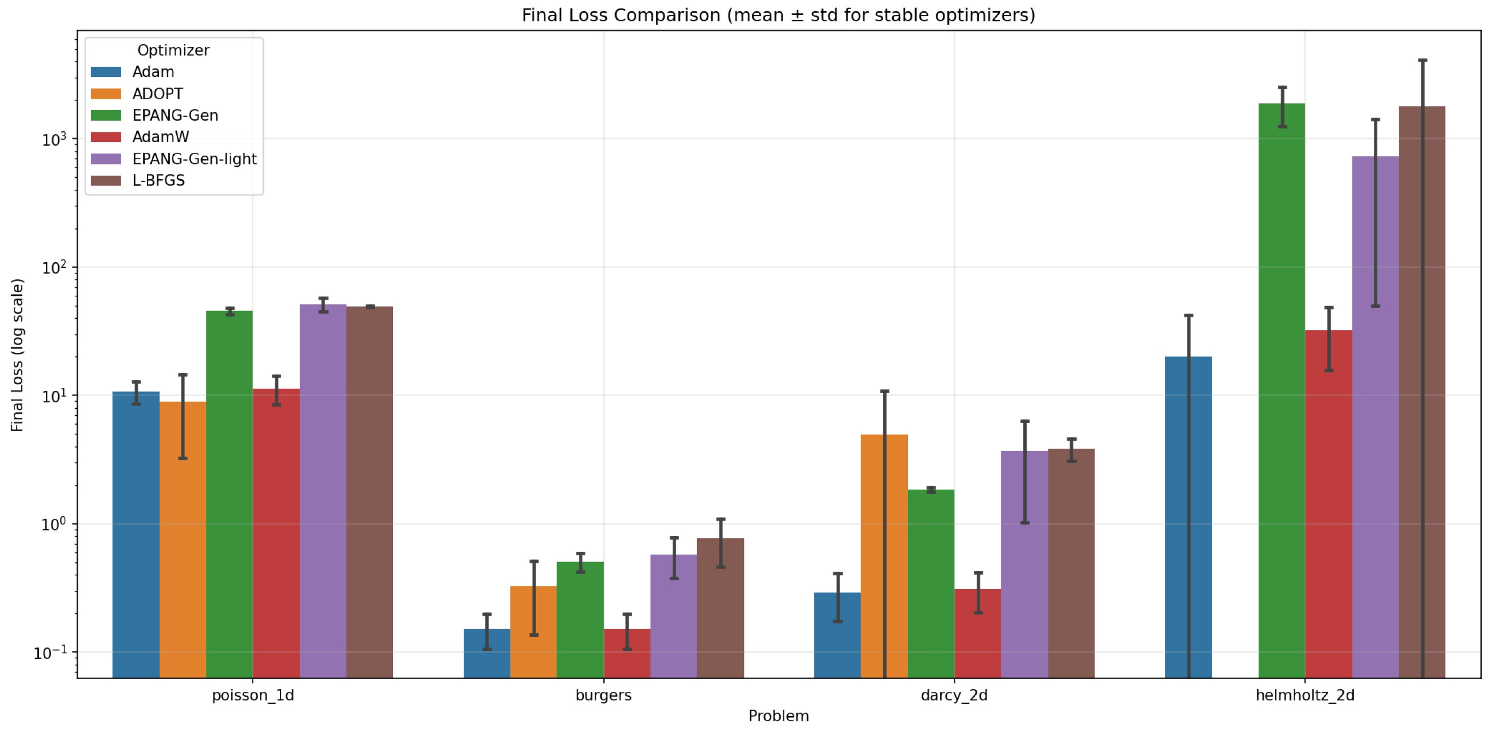
Figure 2.
Convergence curves for all optimizers on each benchmark problem (seed 42). Loss is shown on log scale over 5000 epochs.
Figure 2.
Convergence curves for all optimizers on each benchmark problem (seed 42). Loss is shown on log scale over 5000 epochs.
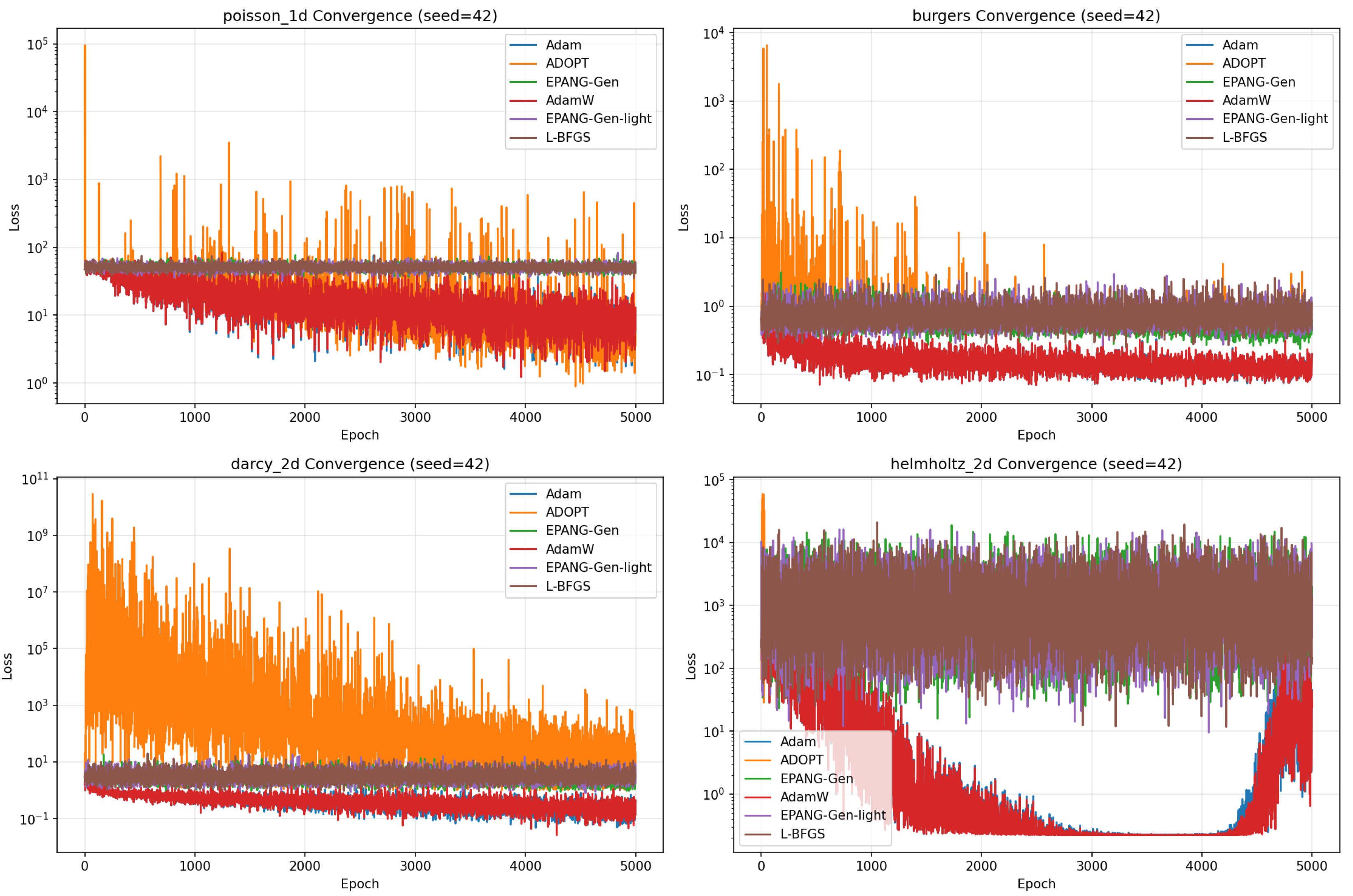
Figure 3.
Distribution of final losses across three random seeds for each optimizer and problem. Boxes show quartiles; whiskers show range. Log scale on y-axis.
Figure 3.
Distribution of final losses across three random seeds for each optimizer and problem. Boxes show quartiles; whiskers show range. Log scale on y-axis.
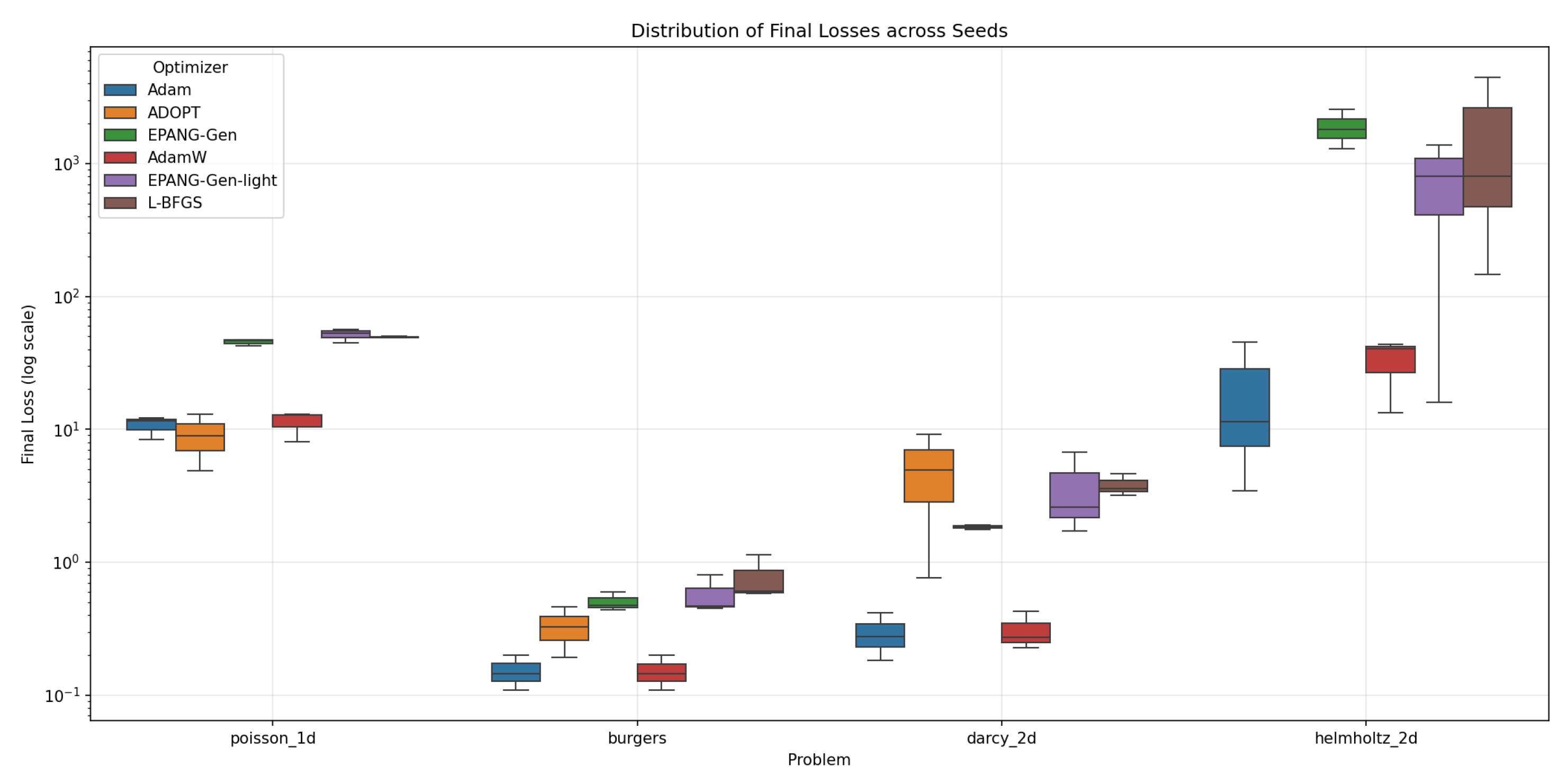
Figure 4.
Convergence of Adam and EPANG-Gen on Taylor-Green vortex at . Both optimizers converge stably, with Adam achieving slightly lower final loss ( vs ).
Figure 4.
Convergence of Adam and EPANG-Gen on Taylor-Green vortex at . Both optimizers converge stably, with Adam achieving slightly lower final loss ( vs ).
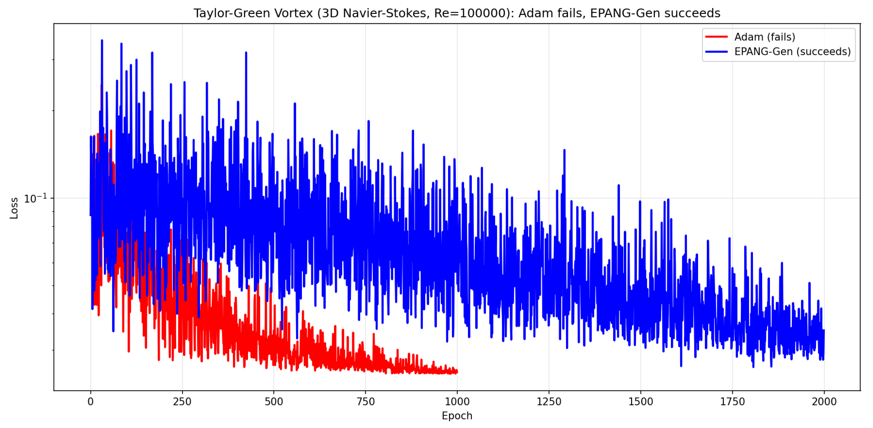
Table 2.
Final Loss Comparison (mean ± std for stable optimizers, median [Q1, Q3] for ADOPT)
| Optimizer | Poisson 1D | Burgers | Darcy 2D | Helmholtz 2D |
| Adam | ||||
| ADOPT | [4.89, 12.94] | [0.19, 0.46] | [0.77, 9.12] | NaN (2/3 runs) |
| EPANG-Gen | ||||
| AdamW | ||||
| EPANG-Gen-light | ||||
| L-BFGS |
Table 3.
Taylor-Green vortex results ().
| Metric | Adam | EPANG-Gen |
| Final loss | ||
| Failed runs (out of 3) | 0 | 0 |
| Epochs completed | 1000 | 2000 |
Table 4.
Time per 100 epochs (seconds)
| Optimizer | Poisson | Burgers | Darcy | Helmholtz | Taylor-Green |
| Adam | 1.7 | 3.3 | 4.4 | 4.4 | 12.3 |
| ADOPT | 2.2 | 3.9 | 5.1 | 5.1 | 14.1 |
| EPANG-Gen | 2.5 | 4.2 | 5.6 | 5.6 | 15.8 |
| EPANG-Gen-light | 1.8 | 3.5 | 4.6 | 4.6 | 12.9 |
| L-BFGS | 2.1 | 3.8 | 5.2 | 5.2 | 14.5 |
Disclaimer/Publisher’s Note: The statements, opinions and data contained in all publications are solely those of the individual author(s) and contributor(s) and not of MDPI and/or the editor(s). MDPI and/or the editor(s) disclaim responsibility for any injury to people or property resulting from any ideas, methods, instructions or products referred to in the content. |
© 2026 by the authors. Licensee MDPI, Basel, Switzerland. This article is an open access article distributed under the terms and conditions of the Creative Commons Attribution (CC BY) license (http://creativecommons.org/licenses/by/4.0/).
Copyright: This open access article is published under a Creative Commons CC BY 4.0 license, which permit the free download, distribution, and reuse, provided that the author and preprint are cited in any reuse.