
Submitted:
03 March 2026
Posted:
05 March 2026
You are already at the latest version
Abstract
This study aims to prove the Riemann Hypothesis and the Generalized Riemann Hypothesis by ex-tending the Riemann zeta function and Dirichlet L -functions to the elliptic complex domain, based ona newly constructed system of elliptic complex numbers Cλ(λ < 0) . The core challenge addressed is theinherent difficulty in resolving these conjectures within the traditional ”circular complex domain” frame-work (λ = −1); the author posits that a complete proof is unattainable strictly within this conventionalsetting.The primary innovation of this work lies in the formulation of the theory of elliptic complex numbers,specifically identifying the limiting case as λ → 0− as the key to the proof. Through rigorous deduction,a bijective correspondence between zeros across different complex planes is established. By employingproof by contradiction and leveraging the correspondence between Cλ (as λ → 0) and the circle complexplane C, the Riemann Hypothesis and the Generalized Riemann Hypothesis are ultimately proven. Thispaper is organized into three parts:(1) Construction and Geometric Properties: The first part details the construction of elliptic complexnumbers and their fundamental geometric properties, laying the necessary foundation for subsequentanalysis and the proof of the conjectures.(2) Analytic Extension: The second part introduces elliptic complex numbers into mathematical anal-ysis, deriving numerous results analogous to those in classical complex variable function theory.(3) Proof of Conjectures: The final part presents the formal proofs of the Riemann Hypothesis and theGeneralized Riemann Hypothesis.
Keywords:
the Riemann hypothesis
; elliptic complex analysis
1. Introduction
In the 1740s, Euler first revealed the connection between prime numbers and functions, establishing the famous Euler product formula:
This formula transformed an additive problem (summation) into a multiplicative one (product over primes), for the first time building a bridge between prime numbers and analytic functions [1].
In 1859, the 32-year-old Bernhard Riemann, in his seminal paper "On the Number of Primes Less Than a Given Magnitude" (originally Ueber die Anzahl der Primzahlen unter einer gegebenen Grösse) [2], treated the zeta function as a function of a complex variable. He proposed two revolutionary ideas:
- (1)
- Using analytic continuation, the domain of the zeta function can be extended to the entire complex plane (except for a simple pole at s = 1). This continued function is what is now known as the Riemann zeta function.
- (2)
- The non-trivial zeros of this analytically continued zeta function determine the precise law governing the distribution of prime numbers [3].
Riemann’s paper, a mere eight pages long, contains profoundly deep insights and opened up entirely new paths for research into the distribution of prime numbers. The function was formally named the Riemann zeta function in his honor.
1.1. The Formulation of the Riemann Hypothesis
Riemann reached the following conclusion in his 1859 paper: the zeros of the Riemann zeta function are divided into two parts:
- (1)
- Real zeros are all negative even integers, i.e., the trivial zeros [1];
- (2)
- There also exist complex zeros, which are distributed in the critical strip . Actually, Riemann originally proposed that the non-trivial zeros lie in the critical strip ; later mathematicians refined this conclusion [4].
In his paper, Riemann presented three propositions [2].
Theorem 1.1.
If we define as the number of non-trivial zeros of with , then
Theorem 1.2.
If we define as the number of non-trivial zeros of on the critical line with , then
These were Riemann’s first and second propositions, which seemed so certain to him. However, the first proposition was only proven 46 years later (in 1905) by the mathematician von Mangoldt [5]. The second proposition was not proven until nearly a century later (in 1942) by the mathematician Atle Selberg [6].
Combining numerous "pieces of evidence," Riemann boldly conjectured: All non-trivial zeros of the function lie on the critical line [3].
When the Riemann Hypothesis was first proposed in 1859, it did not immediately create a sensation [1]. On one hand, Riemann’s paper was exceedingly brief, with many crucial steps "omitted from the proof," making it difficult for mathematicians of the time to fully grasp its profound implications. On the other hand, its conclusions were so ahead of their time that some mathematicians even viewed it with skepticism [7].
However, there was one mathematician who was full of confidence in it, believing that it would be solved within 50 years. This optimist was Charles Hermite [8]. According to some historical sources on mathematics, Hermite expressed this view in letters to friends, showing great optimism about the prospects of the Riemann Hypothesis. History proved him overly optimistic, however, as the conjecture remains unproven to this day.
In 1900, Hilbert delivered his famous lecture at the International Congress of Mathematicians in Paris, presenting the influential "23 Mathematical Problems" that charted the course for 20th-century mathematical research [9]. The Riemann Hypothesis was included as part of Problem 8, alongside other number theory challenges such as the Goldbach Conjecture [10]. It was due to Hilbert’s enormous influence that the Riemann Hypothesis was elevated to an unprecedented status, becoming a towering peak that mathematicians aspired to conquer [11].
Today, of Hilbert’s 23 problems, apart from Problem 8, the remaining 22 problems have either been completely or partially solved, or have been proven to be untenable in certain formulations [10,12]. The Riemann Hypothesis has thus become the most influential and perhaps the most difficult unsolved mystery of all [3,13].
1.2. Important Milestones in the Study
Since Riemann first proposed the hypothesis in 1859, mathematicians have engaged in continuous attempts to prove it [1]. Here we will list only those results that have played a decisive role, hold significant meaning, or even represent the current state-of-the-art conclusions .
1.2.1. The Prime Number Theorem
In 1896, Hadamard and de la Vallée-Poussin independently proved the crucial result that the Riemann zeta function has no zeros on the line [19,20]. From this zero-free region, they were able to prove the Prime Number Theorem, which describes the asymptotic distribution of prime numbers [4]:
where denotes the number of primes less than or equal to x, and is the logarithmic integral function [21].
1.2.2. The Number of Zeros on the Critical Line
In 1905, von Mangoldt proved and obtained the exact formula for the zero-counting function[22], namely the Riemann-von Mangoldt Formula [1,4]:
Furthermore, in 1914, Hardy utilized the function to obtain a proof of Hardy’s Theorem [22,23]:
That is, has infinitely many zeros on the critical line .
Of course, at this time, this was still a non-quantitative result. By 1921, Hardy and Littlewood proved that the number of zeros of the Riemann zeta function on the critical line is at least proportional to the height T [24], i.e.,
laying the foundation for subsequent research on zero-density estimates [6,25,26,27].
1.2.3. Riemann-Siegel Formula
In 1932, the German mathematician Siegel discovered an astonishing secret from Riemann’s manuscripts, which had lain dormant for 73 years [1,28]: Riemann not only proposed the hypothesis based on intuition, but he also personally calculated several zeros, such as and , using computational methods far ahead of the mathematical community of his time [23]. From these cryptic manuscripts, Siegel reconstructed a highly efficient formula for computing zeros [7]:
whose computational complexity is only , far superior to the Euler-Maclaurin formula’s [29].
Building upon this foundation, mathematicians have employed an efficient "double-counting" strategy [30,31]:
- (1)
- Zeros on the Critical Line: Using the Riemann-Siegel formula, we can compute the sign changes of the real function [6]. Whenever changes from positive to negative or from negative to positive, a zero is captured. In this way, we can count that within the range of imaginary parts , at least N zeros are found on the critical line.
- (2)
- Total Zeros in the Critical Strip: Using another known mathematical theorem (the argument principle), we can precisely calculate the total number M of all non-trivial zeros within the rectangular region [33]. This calculation does not depend on the specific locations of the zeros.
If the number of zeros N found on the critical line in the first step exactly equals the total number M of zeros in the entire region calculated in the second step, then an irrefutable conclusion can be drawn: Within this region, all M non-trivial zeros, without exception, lie on the critical line! [3].
1.2.4. Theorem on the Density of Critical Zeros
In 1942, the Norwegian mathematician Atle Selberg achieved a major breakthrough in the study of the Riemann zeta function [6,35]. Using the mollifier method, he carefully constructed the mollifier function
where is the Möbius function and f is a smooth cutoff function [4]. The parameter X is chosen optimally as a power of T.
Using this mollifier function, Selberg further constructed the core inequality [1,23]:
where the notation means that the left-hand side is at least a constant multiple of T for sufficiently large T.
From this inequality, Selberg obtained his celebrated theorem [6]: There exists a constant such that
where is the total number of non-trivial zeros with imaginary part between 0 and T, and is the number of such zeros lying on the critical line .
This result was revolutionary because it was the first time mathematicians could prove that a fixed positive percentage of zeros (not just infinitely many) lie on the critical line [35]. Selberg’s original constant c was very small, but subsequent work by Levinson, Conrey, and others has significantly improved this proportion [25,26,27].
In 1974, Norman Levinson achieved a major breakthrough in the study of the Riemann zeta function [25,36]. Building upon Selberg’s mollifier method, he proved that more than one-third of the non-trivial zeros lie on the critical line [1,23].
Levinson considered a deformation of the function [25]:
where is the Riemann xi function, defined as [4].
Using the mollifier function
with for some , he constructed two core integrals [26]
and obtained the key inequality
where R is a parameter related to the choice of y [25].
Through precise estimates of the integrals I and J, Levinson proved that
and with more careful calculations, he obtained the numerical value .
This result improved significantly upon Selberg’s earlier work, which had only established the existence of a positive proportion without giving a specific numerical value [6]. Levinson’s work opened the door for subsequent improvements by Conrey and others [26,27].
In 1989, Conrey significantly improved this result to; In 2020, Pratt, Robles, Zaharescu, and Zeindler further raised it [37,38] to .
In summary, this is the Critical Line Density Theorem: At least of the zeros lie definitively on the critical line, and this portion of zeros is of the same order as the total zeros.
1.2.5. Ingham Bound
In 1940, Albert Ingham proved the classical result on zero-density estimates, known as Ingham’s Theorem [39,40]:
where is the zero-density function [4,23].
For in particular [40],
The Ingham bound is a foundational result in zero-density estimates, used to control the number of zeros that may deviate from the critical line [1]. This bound remained essentially unimproved for over 80 years [3,41].
1.3. Comparative Study of Leading Research Approaches
From the perspective of analytic number theory, mathematicians can directly improve zero-density estimates, gradually pushing the proportion
towards the ultimate goal of 100% [3,4]. The current best result is obtained by the Levinson-Conrey method [26,27,46].
However, the limit of current methods is approximately 50-60% [3,47], and even advancing by a small fraction may consume decades or even centuries of research effort from the academic community [48]. Even if new methods could be found and eventually push the result to 99%, the final 1% might still be an insurmountable chasm [13].
In fact, even if one could push the result to 100%, i.e., prove that 100% of zeros lie on the critical line, this would not be equivalent to proving the Riemann Hypothesis [1,23].
This is because one would still need to exclude the possibility of exceptional zeros at infinity; such zeros could exist at least one, or even infinitely many [6,25]. Current methods cannot eliminate "sparse but infinite" zeros deviating from the critical line, and therefore entirely new nonlinear or global methods are needed to provide a solution [42,44,45].
The distinction between "100% in density" and "all zeros" is crucial: density results only control the proportion of zeros up to height T, but they do not rule out the existence of a sparse set of zeros off the critical line that grows more slowly than [40]. Such a set could still contain infinitely many zeros, each of which would be a counterexample to the Riemann Hypothesis [3].
Beyond the classical analytic methods, several profound alternative approaches to the Riemann Hypothesis have emerged, drawing connections to algebraic geometry, noncommutative geometry, random matrix theory, and quantum physics [1,3,13].
1.3.1. The Algebraic Geometry Analogy: Weil Conjectures
Another direction is the algebraic geometry analogy, namely seeking possible proof patterns over number fields through the Weil conjectures over finite fields [49,50]. The Weil conjectures over finite fields were proved by Deligne in 1974 [50], and the Riemann hypothesis part of the Weil conjectures is precisely the Riemann hypothesis over finite fields [51].
However, it should be noted that although Deligne’s proof represents the pinnacle of 20th-century mathematics, the essential differences between number fields and finite fields make generalization extremely difficult [52]. This is the fundamental difference between characteristic p and characteristic 0, and the Frobenius endomorphism has no direct analog in number fields [53,54].
1.3.2. Noncommutative Geometry: Connes’ Approach
Another promising direction is noncommutative geometry, which transforms number-theoretic problems into space-spectrum problems [55,57]. Connes conjectured a global trace formula, which is the sum of contributions from local trace formulas; this conjecture is equivalent to the Riemann hypothesis [55,58].
Currently, the local formula has been rigorously proved, but the convergence of the global summation remains unresolved [54,58]. It can be seen that Connes’ method provides the deepest conceptual framework, but the technical details are not yet complete. This may require the development of new tools beyond current noncommutative geometry [54,59].
1.3.3. Random Matrix Theory
In fact, random matrix theory is also a promising approach to studying the Riemann hypothesis [60,61]. Mathematicians use GUE eigenvalue statistics to predict zero distributions and seek deeper structures [62,63].
However, although random matrix theory provides powerful heuristic evidence, it has not yet provided a rigorous path to proving the Riemann Hypothesis [3,13]. This is because the statistical correspondence may be a "coincidence" or "universality" phenomenon, lacking a bridge from statistics to determinism [64].
1.3.4. The Hilbert-Pólya Operator
Another intriguing research direction is the Hilbert-Pólya operator method, whose core strategy is to find a self-adjoint operator H whose eigenvalues correspond to the zeros of the function [65,66]. Scientists hope to construct a concrete quantum Hamiltonian operator and prove a one-to-one correspondence between its spectrum and the zeros; if the operator is self-adjoint, this could further prove the Riemann hypothesis itself [62,66].
Although this method promises that finding the Hilbert-Pólya operator would immediately prove the Riemann hypothesis, no concrete construction has yet been achieved [13]. Moreover, this approach lacks a rigorous correspondence from classical chaos to quantum spectra, requiring an entirely new quantization framework [64,66].
These diverse approaches—algebraic geometry, noncommutative geometry, random matrix theory, and quantum physics—each offer profound insights into the Riemann hypothesis [1,13,54]. While none has yet provided a complete proof, they continue to inspire new mathematical developments and deepen our understanding of the connections between number theory and other areas of mathematics and physics [64,67].
1.4. The Undecidability of the Riemann Hypothesis
In fact, there is a view, which is not mainstream in the mathematical community, that the Riemann Hypothesis (RH) is unprovable. The core idea of this view is that if RH is unprovable, then it must be true. This makes it a potential candidate for the most dramatic instance of Gödel’s Incompleteness Theorems in number theory.
Gödel’s Incompleteness Theorems state that in any sufficiently powerful axiomatic system that contains basic arithmetic such as ZFC , there exist propositions that can neither be proven nor disproven i.e., "independent" propositions . The history of mathematics indeed contains important number-theoretic statements that have been proven independent . For example , the Continuum Hypothesis is independent of ZFC, but is not an arithmetic statement; while Goodstein’s theorem and the Paris-Harrington theorem are arithmetic statements independent of the Peano axioms but provable in ZFC . This invites speculation about whether RH might also be independent of ZFC.
Gregory Chaitin, the founder of algorithmic information theory, is one of the most prominent mathematicians to publicly discuss the idea that the RH might require new axioms.
Chaitin argues that the distribution of prime numbers exhibits a certain "randomness" (pseudo-randomness). In his books and papers, he proposes that the truth of RH may stem from this arithmetic randomness, which, to some extent, resembles the intrinsic randomness of quantum mechanics and cannot be fully captured by a finite, deterministic axiomatic system [32,84]. He speculates that proving RH might require introducing "new axioms," analogous to physical laws, or acknowledging that certain mathematical facts are "accidentally true" rather than logical necessities.
Yuri Matiyasevich proved the undecidability of Hilbert’s Tenth Problem (the solvability of Diophantine equations). He demonstrated how to transform RH into a question about the existence of solutions to a massive Diophantine equation. Matiyasevich suggests that since the general problem of Diophantine equations is undecidable, a specific, extremely complex equation (such as the one corresponding to RH) might also be undecidable within the current axioms [56,85].
As one of the leading figures in contemporary analytic number theory, Brian Conrey holds a more pragmatic attitude towards RH but also acknowledges this possibility. In his renowned survey article, he points out that while the numerical evidence overwhelmingly supports RH, we cannot rule out the possibility that it is unprovable in ZFC. If RH were undecidable, it would be a groundbreaking discovery because it would mean RH is true (as argued above), but we could never prove it within our existing framework [3].
The idea that RH might be unprovable is a fascinating philosophical possibility and a logical fallback, especially in light of the long-standing failure to find a proof. It serves as a reminder that our system of axioms might be insufficient to capture all mathematical truths. However, in practical research, this is more of a "last resort." The current direction of effort remains focused on finding new mathematical tools (such as noncommutative geometry, random matrix theory, and new developments in algebraic geometry) to prove it, rather than proving its unprovability.
1.5. Research Objectives
Regardless of perspective, we must first reach a consensus: it is impossible to obtain a complete proof of the Riemann Hypothesis using only the basic tool of complex numbers.
In fact, looking back at the history of mathematicians’ research on the Riemann Hypothesis, we can observe the following fact: ever since Riemann introduced the function into the complex domain, studied the zero distribution of the function, and proposed formula 1 and the Riemann Hypothesis, mathematicians have become inextricably trapped in the path suggested by Riemann’s formula 1 , embarking on the so-called research journey. However, following this direction, our research is doomed to fail. As analyzed in Section 1.3 , a proof of the Riemann Hypothesis itself is still considered ’miles away’ even if the results are optimized to their theoretical limit . Although it is undeniable that the new tools developed during this research may advance the field of mathematics, I believe that no matter how much progress we make in this direction, it is ultimately meaningless for the Riemann Hypothesis itself.
Although scientists have attempted to find other possible directions, such as using new methods like random matrix theory to study the Riemann Hypothesis, these efforts are largely approached in a spirit of "verification" rather than proof itself. Such approaches seem more like an act of helplessness when unable to find a genuine proof.
Returning to the very beginning of Riemann’s work, i.e., "introducing the function into the complex domain," it might be considered to expand the complex domain, finding algebraic systems parallel to the complex domain, studying the zero distribution of the function in these algebraic systems, and thereby gaining insight into the essence of the Riemann Hypothesis as a whole?
This is the fundamental research approach of this paper. No argument is made regarding whether the Riemann Hypothesis is provable in the complex domain; instead, algebraic systems with properties similar to those of the complex domain—namely, elliptic complex numbers—are directly constructed . Subsequently, the geometric, algebraic, and analytic properties of elliptic complex numbers will be investigated, given their role as essential foundational material for the proof of the Riemann Hypothesis . It should be noted that elliptic complex numbers do not refer to a specific algebraic system, but rather a collection of algebraic systems with properties analogous to complex numbers. In a sense, all elliptic complex numbers, inclusive of ordinary complex numbers, would be regarded as ’variables’ within the scope of this study.
Regarding the proof of the Riemann Hypothesis, this paper will investigate the correspondence of the zero distribution of the Riemann function across the complex planes corresponding to all elliptic complex numbers. From this correspondence, we discover that on one particular complex plane, the Riemann Hypothesis is "self-evident," and this naturally corresponds to all other complex planes, ultimately providing a proof of the Riemann Hypothesis.
Of course, the proof of the Generalized Riemann Hypothesis will also be presented at the end using the same method .
2. Elliptic Complex Numbers and Their Geometric Significance
As a special kind of algebraic system, complex numbers are introduced out of necessity when solving algebriaic questions in the 16th century [68,69].In the mid-16th century, the Italian mathematician Cardan, when solving cubic equations in 1545, first conceived the idea of taking square roots of negative numbers [70,71]. To make square roots of negative numbers meaningful, it was necessary to extend the number system once again, thus introducing the imaginary number . Euler systematically established the theory of complex numbers in 1777, using i to replace as the unit of imaginary numbers [72,73].
In fact, in a broad sense, mathematicians have discovered (invented) three types of binary numbers: complex numbers (hereafter referred to as circular complex numbers to distinguish them), hyperbolic complex numbers (hereafter referred to as equilateral hyperbolic complex numbers to distinguish them), and dual numbers [74,75,76]. Remarkably, all three types of complex numbers satisfy the commutative law and associative law of multiplication; however, only circular complex numbers form a division algebra, while equilateral hyperbolic complex numbers and dual numbers are not divisible [77,78,79].
This chapter will construct a series of generalized binary complex numbers and study their algebraic properties and underlying geometric properties .
2.1. Construction of Generalized Complex Numbers
Based on the three types of binary numbers given by mathematicians [74,75,76], we present the construction of generalized binary complex numbers [77,78,80].
Definition 2.1
In particular, when , this corresponds to equilateral hyperbolic complex numbers; when , this corresponds to circular complex numbers; when , this corresponds to dual numbers [76,77].
The addition and scalar multiplication operations of generalized complex numbers are defined as follows: Let , ,
Two generalized complex numbers and are equal if and only if their corresponding real and imaginary parts are equal, i.e.,
Thus we have the zero element of generalized complex numbers
If the imaginary part of a generalized complex number is 0, i.e., , then it is a real number; if the real part of a generalized complex number is 0, i.e., , then it is called a pure generalized complex number, or pure imaginary number [70,72]. These definitions are consistent with those of circular complex numbers [68,69].
2.2. Operational Rules of Generalized Complex Numbers
This section mainly discusses the rules of multiplication. The rules of addition, through the definitions of addition and scalar multiplication given above, can easily be seen to satisfy associativity, commutativity, and distributivity with respect to real numbers; division operations will be discussed subsequently [76,77].
From Definition 2.1, we obtain the multiplication operation of generalized complex numbers [78,80]
where is the vector form of generalized complex numbers, and
are called the multiplier matrix and inverse multiplier matrix with respect to the product , respectively [79,81].
2.3. Elliptic Complex Numbers
In comparison, we prefer the most familiar real numbers, so no matter how complex the algebraic system we encounter, we tend to find the simplest mapping from that algebraic system to the real numbers [76,77]. Thus,
Definition 2.2
Obviously,
Definition 2.3
(Norm). Let , then is called the norm of the complex number z, i.e.,
When , we always have , and in this case is called the modulus of the complex number z [79,81]. In this case, let , from Equation 3 we obtain
This equation represents an ellipse, showing the geometric interpretation of generalized complex numbers with [76,77]. It can be seen that this is a general equation of an ellipse, whose eccentricity is . Substituting gives
When , which corresponds to circular complex numbers , the eccentricity [78,80]. Therefore, we have the following definition:
Definition 2.4
This classification unifies the geometric interpretation of generalized complex numbers with negative values, with the special case corresponding to the familiar circular complex numbers (ordinary complex numbers) [76,77].
When , from Equation 3 we see that its norm is not positive definite [76,77], and its norm corresponds to
which is the equation of a hyperbola [78,80], with eccentricity consistent with Equation 4. The equilateral hyperbolic complex numbers correspond to , with eccentricity , taking the form of an equilateral hyperbola [76,79].
In general, generalized complex numbers with are collectively called hyperbolic complex numbers [77,81]. Obviously, hyperbolic complex numbers cannot represent points on the asymptotes in the complex plane, because the norm (or modulus) of points on these asymptotes is zero; this is precisely the geometric reason why hyperbolic complex numbers do not form a division algebra [78,80].
To distinguish between them, we stipulate that the imaginary unit for elliptic complex numbers is denoted by i, so they take the form
and the imaginary unit for hyperbolic complex numbers is denoted by j, so they take the form
Subsequent research will mainly focus on the more "perfect" elliptic complex numbers, as they possess positive definite norms and form division algebras, making them more suitable for various applications.
2.4. Euler’s Formula for Generalized Complex Numbers
One might doubt whether the generalized complex numbers defined in this way are meaningful [76,77]. Next, we will further explore the algebraic properties of generalized complex numbers and reveal more of their elegant properties [78,80]. Using methods similar to those for complex numbers (i.e., circular complex numbers), we have the following conclusion.
Proposition 2.5
Proof.
Proposition 2.6
Corollary 2.7.
Following the same procedure, it follows that
which is Euler’s formula in the generalized sense for hyperbolic complex numbers [78,80].
Proposition 2.8
(Exponential Additivity). Let , then .
Proof.
Corollary 2.9.
Analogously, it follows that
2.5. Division Operations for Generalized Complex Numbers
Definition 2.10
Since , elliptic complex numbers have no non-zero zero divisors and form a division algebra [77,79]. As the same way,
Definition 2.11
2.6. Vectors on the Elliptic Complex Plane
Similar to the circular complex plane , we define the vector corresponding to the complex number in the elliptic complex plane as [76,77]. For convenience, unless otherwise specified, in the following we always assume .
This vector representation allows us to study elliptic complex numbers geometrically, with the real part x and imaginary part y serving as coordinates in the elliptic plane [79,81]. The parameter determines the geometry of this plane, with the special case corresponding to the ordinary complex plane [76].
Consider the unit complex number. According to Euler’s formula , it is easy to see that for a point in the complex plane compared to a point on the unit circle in the circular complex plane , its abscissa remains unchanged while its ordinate becomes times the original [76,77]. As shown in Figure 1, here we take as an example.
It is easy to see that . From an ordinary geometric perspective, the modulus of the vector z in the figure is greater than 1, which is the modulus of its corresponding point on the unit circle; however, in the complex plane , the modulus of the vector z is exactly 1 . Similarly, from an ordinary geometric perspective, the angle of the vector z should be , but in , its angle is .
Corollary 2.12
(the Angle in the Elliptic Complex Plane). In summary, the angle α in the complex plane , when measured in the ordinary geometric sense, is β, and they satisfy .
Consider two vectors in the complex plane . Their angles in the ordinary geometric sense are respectively, while their angles in are respectively [81]. Then it follows that
Thus when the angle is , it follows that
This relationship shows how orthogonality in the elliptic complex plane (with angle having difference ) translates to a specific product relationship of the ordinary geometric angles [76,78].
2.6.1. Length and Angle of Vectors on the Elliptic Complex Plane
In order to correctly describe vectors in the complex plane corresponding to the definition of elliptic complex multiplication [76,77], we can introduce the following definitions.
Definition 2.13
By the same token,
Definition 2.14
(Vector Angle). Define the angle between and in by
Now let us analyze the reasonableness of this definition . Let the angles between the vectors and the positive direction of the X-axis in the coordinate system corresponding to the elliptic complex plane be respectively [78,80]. Then when ,
Obviously, Equation 9 satisfies the trigonometric identity [79,81]. Furthermore, from Equation 7 it is easy to obtain the unit vectors of and as
According to Equation 8 combined with Equation 7, we have , that is
This is consistent with the result in trigonometric identities [76]. It can be seen that such a definition is reasonable.
Based on Equation 6, the vectors and in the complex plane are perpendicular to each other [78]. In this case, from Definition 2.13 we know that , thus we have the conclusion:
Proposition 2.15
2.6.2. Right Angles on the Elliptic Complex Plane
As mentioned above: from an ordinary geometric perspective, the angle of the vector should be , but in , the magnitude of this angle is [76,77]. The angle between two vectors in the complex plane defined above is precisely the magnitude of in [78,80]. Now we determine the value of the aforementioned in the ordinary geometric sense, i.e., the value of in the circular complex plane , denoted as [79,81].
For the unit vectors in Equation 10, their angle in satisfies
Based on Equation 11, when , i.e., , it can be shown that . This means
Corollary 2.16
If the vectors are mutually perpendicular in the elliptic complex plane , then from equation (1.18) we know that [80]. Substituting this into Equation 11 yields
It can be seen that even for two vectors that are mutually perpendicular in the complex plane , their angle in the circular complex plane will vary with changes in or [79,81]. Therefore it leads to
Corollary 2.17
This result highlights a fundamental difference between elliptic complex geometry (with ) and Euclidean geometry: while straight lines remain straight under the transformation between different planes, the measure of angles, particularly right angles, is not preserved in a uniform way [76,80].
It is well known that one of the five postulates of Euclidean geometry states: "All right angles are congruent to one another" [68,69]. Clearly, the geometry corresponding to elliptic complex numbers does not satisfy this postulate [77,81]. This result demonstrates that the geometry induced by the elliptic complex plane with (i.e., ) is non-Euclidean [76,78].
2.7. Geometric Significance of Elliptic Complex Numbers
For a point in the elliptic complex plane , let the coordinate origin be O [76,77]. Then the corresponding vector is , with [78,80]. Now consider the vector
so the coordinates of point B are [79,81]. As a result,
which yields the same result as Equation 6 [78]. In particular, if we set , then A is exactly a point on the positive X-axis, and B is exactly a point on the positive Y-axis. It can be seen that when , the angle between the positive X-axis and the positive Y-axis in the complex plane is no longer a right angle [80]. Consequently,
Corollary 2.18
Furthermore, consider the vector [76,77]. Obviously, in the complex plane , we have and [78,80]. Consequently,
Corollary 2.19
(Orthogonal Equal-Length Vectors). Two vectors in the complex plane are mutually orthogonal and of equal length if and only if
This is the geometric interpretation of the correspondence between a complex number (or vector) z and the complex number (or vector) in the complex plane [79,81].
2.7.1. Normal Ellipse
Just as the definition of a "circle" in the circular complex plane , we also need to find analogous geometric elements in the elliptic complex plane [76,77].
From the definitions of norm and modulus for elliptic complex numbers , we have [78,80]
whose geometric interpretation is an ellipse centered at the coordinate origin in the complex plane [79,81]. When , the semi-major axis length of this ellipse is , and the semi-minor axis length is ; when , this ellipse degenerates into a circle with radius , which is the geometric interpretation of circular complex numbers; when , the semi-major axis length is , and the semi-minor axis length is [76,78].
This type of ellipse, which can define the norm or modulus in the complex plane , possesses very essential characteristics [77,80]. To fully characterize this geometric element, we first give the following definitions:
Definition 2.20.
When , the direction of the minor axis of the ellipse is its principal axis direction, and the direction of the major axis is its secondary axis direction; when , the direction of the major axis of the ellipse is its principal axis direction, and the direction of the minor axis is its secondary axis direction [78,79].
Definition 2.21.
Combined with Equation 4, The following definition is established.
Definition 2.22
2.7.2. Representation of Normal Ellipses on the Complex Plane
Let [78,80]. Then . Hence it leads to the complex equation of a straight line [79,81]
that is
where . This is the equation representation of a straight line in the elliptic complex plane [76,78].
Now we discuss the representation of a normal ellipse in the complex plane [77,80]. Since
so represents a normal ellipse centered at [79,81].
Let a normal ellipse in the complex plane be . Squaring both sides and expanding gives
That is, the equation of a normal ellipse in the complex plane is
where when , the equation degenerates into the form of a straight line equation [78,80]. Therefore, the normal ellipses and the straight lines in the complex plane are unified, with a straight line being a normal ellipse with infinite principal radius [76,79].
2.7.3. Limiting Cases of Elliptic Complex Numbers
Proof.
From this, we can see
Corollary 2.24
It should be noted that, as shown in Figure 2 , the angle tending to 0 does not mean that the X-axis and Y-axis coincide [76,77]. The region between the positive X-axis and the positive Y-axis, as shown in (1) of the figure, still contains infinitely many points [78,80], and there is a one-to-one correspondence with the points in the region between the positive X-axis and the positive Y-axis in the orthogonal plane shown in (2) of the figure [79,81].
Furthermore, the geometric interpretation of the complex plane as is shown in Figure 3 [78,80]: the corresponding complex plane represents an oblique coordinate plane where the angle between the positive Y-axis and the positive X-axis tends to [79,81].
In fact, it is difficult to determine the exact angle between the positive Y-axis and the positive X-axis for the coordinate system corresponding to each complex plane [76,77]. What we can determine is that as , the plane reaches a "sufficient limit" that allows us to glimpse the essential properties within the "black box" of elliptic complex numbers [78,80].
2.8. Conclusion
It should be noted that mathematicians have already given certain special "elliptic complex numbers" in the algebraic sense, such as the integral domains , , etc., as well as imaginary quadratic fields , where d is a negative square-free integer. However, mathematicians tend to study the algebraic properties corresponding to these special "elliptic complex numbers," and even more so, to explore the properties of divisibility at present .
In a sense, this behavior of mathematicians is more like studying the discrete mathematical structures of "elliptic complex numbers." But the Riemann Hypothesis itself belongs to the realm of analysis. We naturally hope to construct a series of "continuous" algebraic structures, and even treat these algebraic structures as parameters, to study the zero distribution of the Riemann function holistically using the tools of mathematical analysis.
From a purely algebraic perspective, elliptic complex numbers are algebraically isomorphic to circular complex numbers. From a geometric perspective, however , elliptic complex numbers represent geometric elements in a Cartesian coordinate system that have been transformed from an oblique coordinate system.
It is important to note that we require to be a constant. The reason is that to solve the proof of the Riemann Hypothesis itself, letting be a constant is sufficient. As for further research on the distribution of zeros on the critical line, it may require designing special elliptic complex numbers to resolve. In fact, if is a function of one or more variables , then it corresponds to a curved or even surface coordinate system. This would then correspond to geometry in curved spaces.
On the other hand, we consider the case , which does not mean that is a variable. Its true meaning is that equals a constant approaching 0. It can be seen that the elliptic complex numbers with also form a number field, corresponding to an oblique coordinate plane where the angle between the positive Y-axis and the positive X-axis tends to 0. However, it is particularly important to note that the elliptic complex numbers at this point still represent geometric elements in a Cartesian coordinate system.
In fact, using elliptic complex numbers allows us to appreciate the unique charm of observing a geometric object from different geometric perspectives. As is well known, the world in our human eyes is completely different from the world as seen by other creatures such as cats, dogs, etc. Are there civilizations in the universe that are similar to us or even more advanced than us ? What differences would there be between the physical world observed by these civilizations and that observed by us humans? Elliptic complex numbers are precisely what we need to predict our physical world from all these possible perspectives.
As demonstrated, elliptic complex numbers essentially provide an alternative formulation for calculating vector lengths within the defined space. While this definition is fundamentally simple, it possesses the potential to profoundly reshape our conceptual framework for understanding the physical world. The author posits the significant value of this approach and anticipates its validation and further exploration by the broader scientific community.
Part I
Mathematical Analysis on Elliptic Complex Numbers
3. Theory of Elliptic Complex Functions
3.1. Ellipsoidal Representation of Elliptic Complex Numbers and the Extended Complex Plane
In the plane, there is no point corresponding to ∞ [76,77]. Of course, we can introduce an "ideal" point, called the point at infinity [68]. All points in the plane together with the point at infinity form the extended complex plane [69]. We stipulate that every straight line passes through the point at infinity; consequently, there is no half-plane that contains this ideal point [78]. Previously, we unified normal ellipses and straight lines through their equations [80].
In fact, the unification of normal ellipses and straight lines can be achieved by introducing the point at infinity, which leads to the concept of a complex ellipsoid [79,81].
Definition 3.1
(Ellipsoid and Polar Projection). Consider in the three-dimensional rectangular coordinate system the ellipse If we rotate C around the X-axis, we obtain a rotational ellipsoid
The vertex of is called the X-system pole of the ellipsoid, denoted by [78,80]. For any point on , draw the line connecting and and extend it; it necessarily intersects the coordinate plane at a point [79]. We call the X-system ellipsoidal polar projection of , and the correspondence is called its X-system ellipsoidal polar mapping [81].
Now we find the correspondence relation for [76,77]. Let and , with its corresponding point in the complex plane being [78]. From geometric relations we obtain
Thus
Conversely,
and
Definition 3.2
(Y-System Ellipsoid and Polar Projection). If we rotate C around the Y-axis, we obtain a rotational ellipsoid
The vertex of is called the Y-system pole of the ellipsoid, denoted by [76,77]. For any point on , draw the line connecting and and extend it; it necessarily intersects the coordinate plane at a point [78,80]. We call the Y-system ellipsoidal polar projection of , and the correspondence is called its Y-system ellipsoidal polar mapping [79,81].
Now consider the X-system pole (or the Y-system pole ) [76]. Clearly, (or ) corresponds to the point at infinity in the complex plane [68,69]. Thus we introduce a new elliptic complex number ∞ corresponding to it. The complex plane together with this point forms the extended complex plane, or complex ellipsoid, denoted by [78,80]. The operations for this new elliptic complex number ∞ are defined as follows:
3.2. The Topology of the Elliptic Complex Plane
As established in Section 2.7.1, the normal ellipse is the fundamental tool for describing the magnitude and direction of vectors on the elliptic complex plane. Similar to the method for the circular complex plane, we now use normal ellipses to analyze the topological structure within the elliptic complex plane [78,80].
Definition 3.3
From the properties of neighborhoods around a point, we have:
Definition 3.4
(Limit Point, Interior Point, Boundary Point). Let and . Then,
If but is not a limit point of E, then it is called an isolated point of E [78]. The set of all boundary points of E is called the boundary of E, denoted by ; the set is called the closure of E [80].
Definition 3.5
Definition 3.6
(Region). Let D be a point set in the complex plane satisfying
It can be seen that a region is a connected open set [77]. If a region together with its boundary is considered, it is called a closed region [76].
Definition 3.7
A simple continuous curve is called a Jordan curve [76,77]. A simple continuous closed curve (with its endpoints coinciding) is called a Jordan closed curve (or simple closed curve) [69,78].
Definition 3.8
(Jordan Curve Theorem for ). Any simple closed curve divides the complex plane into two regions with no common points [76,80], one of which is a bounded region (called the interior region) and the other is an unbounded region (called the exterior region) [77,79], and both regions share this closed curve as their common boundary [78,81].
Definition 3.9
These definitions establish the fundamental concepts of connectivity in the elliptic complex plane , analogous to those in the standard complex plane [69,81]. The Jordan curve theorem ensures that every simple closed curve has a well-defined interior and exterior, which is essential for understanding the topological structure of regions in and for the subsequent study of elliptic complex functions, their continuity, and limits [78,80].
3.3. Elliptic Complex Functions: Continuity and Limits
The definition of elliptic complex functions is, in form, actually the same as the definition of functions in mathematical analysis and in (circular) complex function theory studied by mathematicians [76,77].
Definition 3.10
Just like circular complex functions, elliptic complex functions also have single-valued and multi-valued complex functions [79,81]. If there is a uniquely determined w corresponding to it, it is a single-valued complex function; if there are multiple or infinitely many w corresponding to it, it is a multi-valued complex function [78]. For now, the complex functions we refer to are all single-valued complex functions.
From the definition, we have [80]. To describe the graph of , we would need to use four-dimensional space (which is clearly beyond our imagination) [76]. To avoid this difficulty, we use two complex planes: the z-plane and the w-plane [77]. We understand complex functions as mappings between point sets in these two complex planes [79,81].
Definition 3.11
Definition 3.12
As a result, we have the following conclusion.
Proposition 3.13
Proof.
Note that q is a nonzero constant [78]. Hence,
⇒: Since , the first inequality gives the result;
Definition 3.14
(Continuity of a Function). Let be a complex function defined on a point set E, let be a limit point of E, and [76]. If
Proposition 3.15
Analogously, the four arithmetic operations are closed for continuous functions, i.e., if and are continuous at , then the functions
are also continuous at [78,79].
Definition 3.16
It should be noted that continuity is a local property, generally concerning a single point, while uniform continuity is a global property [79,81].
Theorem 3.17
Theorem 3.18
Theorem 3.19.
Definition 3.20
3.4. Derivatives of Elliptic Complex Functions and Analytic Functions
Based on the above discussion, we begin to explore the differential structure of elliptic complex functions [76,77].
3.4.1. Basic Concepts of Analytic Functions
Definition 3.21
The quantity is called the differential of at z, denoted by or , i.e., [79,81]. In fact, from the properties of differentials, the function is differentiable at if and only if
Definition 3.22
(Analyticity). Let be a single-valued complex function defined on a region D, and let [76,78]. If there exists a neighborhood of such that is differentiable at every point in this neighborhood, then the function is said to be analytic at [77,80]. If the function is analytic at every point in the region D, then is said to be analytic in the region D [79,81].
It can be seen that differentiability is a local concept, while analyticity is a global concept [76,77]. A function may be differentiable at a point without being analytic there, but if it is analytic at a point, it must be differentiable there [78,80]. Analyticity in a region is equivalent to differentiability in that region [79,81].
Similarly, the four arithmetic operations are closed for analytic functions, i.e., if and are analytic in a region D, then the functions
are also analytic in the region D, and it is obtained that
3.4.2. The C.-R. Equations for Analytic Functions
We know that a real-valued function of two variables is differentiable at a point if there exist numbers independent of such that [76,77]
where [78,80]. In this case, , , and [79,81].
Let be a complex function defined on a region D[76]. When and are given, the function is also determined. However, in general, if and are independent of each other, even if the partial derivatives of and with respect to x and y exist, the function may not be differentiable [77,78].
Theorem 3.23
(Cauchy-Riemann Equations for Elliptic Complex Analytic Functions). Let be a complex function defined on a region D in the complex plane [79,80]. Then is differentiable at if and only if the functions and are differentiable at and satisfy
where q satisfies () [81]. Equation (2.11) is called the Cauchy-Riemann equations (abbreviated as C.-R. equations) for elliptic complex analytic functions [76,78].
Proof.
□
Substituting Equation 13 into Equation 14 yields other forms of the derivative of the complex function [76,77]. If we set , the C.-R. equations can also be written as [78,80]
3.5. Elementary Univalent Elliptic Complex Functions
Next, several fundamental elementary functions in elliptic complex analysis shall be derived based on the Cauchy-Riemann equations.
3.5.1. Exponential Function
Similar to the exponential function in real analysis, the exponential function in elliptic complex function theory should satisfy the following conditions [76,77]:
- (1)
- When restricted to the real numbers, for , ;
- (2)
- (3)
- , .
From (1) and (3), [79,81]. Then from (2), we know that and must satisfy the Cauchy-Riemann equations [76], giving
with particular solutions , [78,80]. Thus we have the definition of the exponential function:
Definition 3.25
(Exponential Function). Let . The exponential function in the elliptic complex function domain is defined as
Obviously, the elliptic complex exponential function possesses properties as elegant as those of the (circular) complex exponential function [76,81].
Proposition 3.26
For , .
Proof.
Proposition 3.27
, . The function is analytic in the entire complex plane, and .
Proof.
From the definition of the exponential function, let [77]. Then the functions and are differentiable [79], and
As is evident from the above, the C.-R. equations are satisfied, which implies the analyticity of the function in the entire complex plane, and
In summary, the proposition is proved . □
Proposition 3.28
3.5.2. Trigonometric Functions
Consequently,
Definition 3.29
Proposition 3.30
Proof.
Proposition 3.31
Proposition 3.32
Proposition 3.33
Proof.
Therefore, when extending the sine and cosine functions to the elliptic complex domain, their zeros do not increase [78,80].
Proposition 3.34
- (1)
- (2)
From the definitions of the sine and cosine functions [76,77], we can further define other trigonometric functions.
Definition 3.35
It can be seen that the singularities of the function are precisely the zeros of , and the singularities of the function are precisely the zeros of [76,77]. Furthermore, we have
Definition 3.36
It is easy to see that the functions and , like , both have period [78,80], are analytic on [79,81], and satisfy
These two formulas have many applications in the derivation of relevant formulas in subsequent series of articles on the Riemann Hypothesis in the elliptic complex domain [78,80]. The proof of the formulas can be obtained from the basic definitions; readers are encouraged to attempt it themselves [79,81].
3.6. Elementary Multivalent Elliptic Complex Functions
The preceding discussion has focused exclusively on single-valued complex functions; we now turn our attention to multivalued complex functions.
3.6.1. The Argument and Logarithm Functions
It can be seen that the definition of the argument function in the field of elliptic complex functions is consistent with that in the field of circular complex functions [76,77], namely:
Definition 3.37
(Argument Function). When , we call
The above region can be viewed as a region obtained by cutting the entire complex plane along the negative real axis [79,81], where the negative real axis is called a cut line, serving as the boundary of the region D. In general, we take an unbounded simple continuous curve K connecting the origin O to the point at infinity ∞ as a cut line, obtaining a region , called a slit region, whose boundary is the curve K [76,77].
Let , with , take , and consider a simple continuous curve in E connecting and [78,80]. As z moves continuously from to along , also changes continuously from to . Thus, starting from the value of at , we can determine the values at any other position in E, thereby obtaining a single-valued continuous function in E, i.e., a single-valued continuous branch [79,81].
In fact, for a fixed , is also a single-valued continuous branch of the argument function, showing that the argument function is a multi-valued function [76,77].
Proposition 3.38
(Addition and Subtraction Properties). Let , then
Definition 3.39
Now we need to derive the formula for the logarithmic function .
Let (this definition is chosen for the convenience of later definitions of power functions and root functions) [76,77], and . Then from it can be shown that
so , i.e.,
Equation 15 is called the logarithmic function of z [78,80]. Due to the (infinite) multi-valuedness of the argument function, the logarithmic function is also multi-valued [79,81]. In fact, the inverse function of the logarithmic function, namely the exponential function, is periodic, so the logarithmic function is multi-valued [76,77].
From , we call the principal value of the logarithm of z [78,80]. Then
which shows that non-zero complex numbers have infinitely many logarithms, and any two values differ by an integer multiple of [79,81].
Proposition 3.40
It can be seen that for the logarithmic function [78,80], taking each fixed k, the function is a single-valued continuous branch on the slit region [79,81]. Thus we have the following property:
Proposition 3.41
3.6.2. Power and Root Functions
Definition 3.42
From the single-valuedness of the logarithmic function and the analyticity of rational expressions, it follows that the single-valued transformation branches of the power function are also analytic [79,81].
4. Integral Theory of Analytic Functions
In the previous articles, we studied some fundamental theories of elliptic complex functions, including analytic functions, elementary analytic functions, and the Cauchy–Riemann equations. Building on this foundation, this chapter delves into another very important theory—contour integration.
4.1. Fundamental Theory of Contour Integration
4.1.1. Basic Concepts and Conclusions of Integration
Let C be a simple curve (smooth or piecewise smooth) in the complex plane connecting to z, and let the function
be continuous on C. Insert partition points on the curve C: [79,81]. Let , , . Arbitrarily take
and form the sum:
where q satisfies .
Denote . Then as ,
The above limit is defined as the (contour) integral of the function along the curve C, denoted by [76,77]. That is,
Consider expressing the curve in parametric form. Let the simple curve . Then
In summary, it yields the following conclusion.
4.1.2. Basic Properties of Integrals
According to the definition of the integral of elliptic complex functions, its general properties can be easily derived [79,81].
Corollary 4.2
(Properties of Integrals). Let the functions be continuous on the curve C. Then
- (1)
- , where α is a complex constant;
- (2)
- (3)
- , where the curve C is composed of smooth curves connected together;
- (4)
- (5)
- If on the curve C we have , and L is the arc length of the curve C, then we have the integral (estimation) inequality
Proof.
Here we only prove Item 5. From the definition of the integral,
Proposition 4.3
(Fundamental Integral). Let C be the ellipse , oriented counterclockwise. Hence,
Proof.
Owing to , i.e., , we have
When , the integral is
When , the integral is
4.2. Cauchy Integral Theorem
Definition 4.4
If and are both primitive functions of in the region D, then
Hence with and . From this, if a function defined in a region has a primitive function, then it necessarily has infinitely many primitive functions, and any two differ by a constant c [78,80].
Let be a primitive function of in the region D. Then its indefinite integral is expressed as
4.2.1. Three Lemmas
Lemma 4.5
(Polygon Boundary Integral). Let the function be analytic in a simply connected region D, and let C be any polygonal boundary in D. Then
Proof.
Lemma 4.6
(Existence of Primitive Function in Convex Regions). Let the function be analytic in a convex region D. Then necessarily has a primitive function in the region D.
Proof.
Since D is a convex region, for any two points in D, the line segment connecting them must lie entirely in D. Define
Let . By Lemma 4.5, if the function is analytic in a simply connected region D and C is any polygonal boundary in D, then . Hence
The function is analytic in D, i.e., is continuous in D. Thus , such that , and when there exists [76,77].
When , it yields . Then
Lemma 4.7
(Integral with Primitive Function). Let be a continuous function in the region D, and suppose it has a primitive function in D. If two points , and C is a simple curve in D connecting α and β, then
4.2.2. Cauchy Integral Theorem and Related Conclusions
Theorem 4.8
(Cauchy Integral Theorem). Let be an analytic function in a simply connected region D in the complex plane .
- (1)
- Let C be any simple closed curve in the region D. Then
- (2)
- Let C be any simple curve in the region D connecting and z. Then the value of the integral from to z along C does not depend on the path C, but only on and z themselves.
This is the Cauchy Integral Theorem. In fact, conclusion (2) is a corollary of conclusion (1); it suffices to prove (1) [76,77].
Proof.
For , such that the elliptic disk . By Lemma 4.6, has a primitive function on the convex region , and for any two points in , by Lemma 4.7,
In view of the fact that C is a bounded closed curve (i.e., compact), there exist finitely many open elliptic disks in D that completely cover C[78,80]. Choose points . Clearly, has primitive functions on the convex regions . Let denote the line segment, and let denote the curve segment along C from to . Subsequently, by Lemma 4.5,
□
Alternatively, Cauchy’s theorem can be proved using Green’s formula and the C.-R. equations [79,81]:
Proof.
Let , . Since is analytic in D, and are differentiable in D. By Green’s formula
combined with the Cauchy-Riemann equations, it can be shown that
and
Therefore,
This proves the proposition. □
Corollary 4.9.
Theorem 4.10
Proof.
By Theorem 4.8, the integral is path-independent. Define the primitive function as
Then . Hence for ,
Now consider multiply connected regions.
Theorem 4.11
(Cauchy’s Theorem for Multiply Connected Regions). Let there be simple closed curves , where each of the curves lies in the exterior region of the remaining curves, and all lie in the interior region of . That is, together with encloses a multiply connected region D whose closure is . If the function is analytic on the region , then
where is the entire boundary of region D. This conclusion is equivalent to
Combined with Proposition 4.3, it could be shown as the following conclusion.
Corollary 4.12.
Let C be a simple closed curve containing α. Then
Note that if is an analytic function in a multiply connected region D, and we define its primitive function as , then may be a multi-valued function [76,77]. This is because two simple curves in a multiply connected region D from to z may not be able to be combined into the same simple curve within D (with the same starting point). Take a simply connected subregion in D, where . Let be a fixed simple curve in D from to z. Define the function
4.3. Cauchy’s Integral Formula
We know that represents a normal ellipse centered at in the complex plane [79,81]. For simplicity, let the normal ellipse be , i.e., the parametric equation . Then by the symmetry of the ellipse, its perimeter is
Let , and let the principal radius of the ellipse be r. Clearly, . Then when , , and the ellipse perimeter is
When , , and the ellipse perimeter is
Here,
are called the contour coefficients of the normal ellipse in the complex plane when and when , respectively, collectively referred to as the contour coefficients of the complex plane [76,77]. Clearly, for a given complex plane , its contour coefficient is a definite constant. When , we have the classical complex plane , and the contour coefficients [78,80].
Now we proceed to derive the integral formula from the integral theorem.
Proposition 4.13
(Cauchy Integral Formula). Let D be a bounded region with boundary consisting of finitely many simple closed curves C, and let the function be analytic on the closed region consisting of D and C. Then for ,
Proof.
For any point z in D, draw an elliptic circle such that the closed elliptic disk enclosed by lies entirely within D [79,81].
Since is continuous at , for , such that when ,
Therefore, when , if ,
if ,
In summary, since for a given , and are nonzero constants, it leads to
This is the Cauchy integral formula, which can also be written as
Proposition 4.14
(Mean Value Theorem). Let be analytic on the elliptic disk enclosed by . Then
4.4. Cauchy’s Integral Formula for Derivatives of Arbitrary Order
Now, we need to derive the higher-order Cauchy integral formula based on the above integral formula, as stated in the following proposition:
Proposition 4.15
(Higher-Order Cauchy Integral Formula). Let D be a bounded region with boundary consisting of finitely many simple closed curves C, and let the function be analytic on the closed region consisting of D and C. Then has derivatives of all orders in D, and
Proof.
For any , such that . Let , and let L be the arc length of C. Then when ,
Therefore,
Now use mathematical induction to prove the general case [78,80]. Assume the conclusion holds for , i.e.,
Then for ,
Hence,
Corollary 4.16.
The higher-order Cauchy integral formula can also be rewritten as
4.5. Applications of Cauchy’s Theorem
Proposition 4.17
(Cauchy’s Inequality). Let the function be analytic on the closed elliptic disk bounded by , and let . Thereafter,
Proof.
When ,
In particular, when , we have , which is the case of circular complex functions [76,77]. Formula 26 is also called Cauchy’s Inequality.
Definition 4.18
Proof.
Let be a bounded function, i.e., such that for all . Then for any and any , when ,
when ,
By the same token, in the elliptic complex domain, there is also a corresponding Fundamental Theorem of Algebra [78,80].
Proposition 4.20
(Fundamental Theorem of Algebra). Any algebraic equation of degree n
Proof.
Proposition 4.21
(Morera’s Theorem). If the function is continuous in the region D, and for every simple closed curve C in D it leads to
5. Series Representations of Analytic Functions
Clearly, the definitions of complex series and the related theory of series convergence in the elliptic complex domain are the same as the corresponding basic theory in the circular complex domain, so we will not repeat them here (interested readers can refer to relevant materials on (circular) complex function theory) [76,77]. We will start directly from the theory of Taylor series [78,80].
5.1. Taylor Expansion of Analytic Functions
Definition 5.1
(Power Series). Let and be complex constants in the complex plane . Then
5.1.1. Basic Theory of Power Series
Proposition 5.2.
Proof.
In fact, if (1) is true, then (2) must be true [76,77]. Assume (2) is false, then the power series diverges at , and there exists some point in the region outside the elliptic disk satisfying such that the series converges. Then by (1), for any point z in the elliptic disk region satisfying (clearly including ), the series converges, contradicting the assumption [78,80]. Therefore, we only need to prove (1).
Owing to the series converges, by the necessary condition for convergence: , there exists a constant such that
Therefore, for any point z in the elliptic disk region satisfying , it can be seen that
Proposition 5.3
- (1)
- (2)
- (3)
Proof.
Proposition 5.4
(Convergence Radius Formulas). If any of the following conditions holds:
- (1)
- (2)
- (3)
5.1.2. Basic Theory of Taylor Series
Proposition 5.6
Proof.
From Proposition 5.6, we can arrive at the Taylor expansions (at ) of basic elementary functions [76,77]:
and so on.
Proof.
Likewise, we can obtain the Taylor expansion (at ) of the logarithmic function [78,80]. Clearly, is an infinitely multi-valued function, with branch points at [79,81]. Cutting the z-plane along the negative real axis from to ∞, in the resulting region G, the function yields infinitely many single-valued analytic branches [76,77]. Taking the principal value branch , in view of
the Taylor coefficients are
so it leads to
Consequently , the Taylor expansion of at is
In the same manner, we can obtain the expansion of the principal value branch of the function [78,80]:
□
5.2. Isolation of Zeros and Uniqueness Theorem of Analytic Functions
5.2.1. Zeros of Analytic Functions
In many practical problems, it is often necessary to find points where a function equals zero, i.e., to determine roots [76,77].
Definition 5.7
Proposition 5.8
For example, find all zeros of the function [76,77]. Setting , we have
so the zeros are . Due to the fact that
Proposition 5.9
Proof.
5.2.2. Uniqueness Theorem
Lemma 5.10
Proof.
Suppose at some point in D, there exists a neighborhood such that . Arbitrarily take , connect and z with a finite polygonal line L in D, such that the distance between L and the boundary of D is greater than , ensuring that every point on L has some neighborhood contained in D[78,80]. On L, take successively
such that , and the neighborhood of contains , the neighborhood of contains , ..., the neighborhood of contains . Then , so . Hence
From Proposition 5.9 , for a non-identically zero analytic function , its zeros must be isolated; if the zero is isolated, then the function [76,77]. Furthermore , the conclusion below follows. [78,80].
Proposition 5.11
Corollary 5.12.
5.3. Laurent Expansion of Analytic Functions
Let the convergence radii of the two power series be R and respectively [79,81]. Then series 33 converges in , while series 34 converges in , i.e., in [76,77].
Therefore , when , the series
converges in the elliptic annulus [78,80]. Series 35 is called a Laurent series (expansion), where series 33 is called the analytic part of the Laurent expansion, and series 34 is called the principal part of the Laurent expansion [79,81].
Proposition 5.14
(Laurent Expansion). Let the function be analytic in the elliptic annulus . Then in U, has the expansion
and this expansion is unique , where
Proof.
Arbitrarily take . Then there must exist and such that
For , it is concluded that , so
For , we have , so
Therefore,
For the part , let . Then when , we have . Hence,
Combined with the Cauchy integral theorem, it follows that
which gives the conclusion [76,77]. Regarding the uniqueness of the expansion, consider another possible Laurent series with coefficients . By formula 36 [78,80],
By the basic property of integrals as shown in Proposition 4.3 of Section 4.1.2, holds for all k. Hence the Laurent expansion is unique [76,77]. □
5.4. Isolated Singularities of Analytic Functions
Definition 5.15
5.4.1. Basic Theory of Isolated Singularities
Definition 5.16
(Isolated Singularity). If the function is not analytic at , and there exists a punctured elliptic disk
The difference between a singular point and an isolated singular point is that in any neighborhood of a singular point, there are points where is analytic, but the function may not be analytic throughout that neighborhood. An isolated singular point requires the existence of such a punctured neighborhood where is entirely analytic [76,77].
Definition 5.17
(Classification of Isolated Singularities). Let be an isolated singular point of the function . Regarding the Laurent coefficients being zero, there are three cases [78,80]:
- (1)
- (2)
-
If only finitely many have , then is called a pole of . If there exists a positive integer m such that while for all , then is called a pole of order m of , i.e.,
- (3)
Proposition 5.18
(Characterization of Removable Singularities). Let be an isolated singular point of the function . Then is a removable singular point of if and only if
Proposition 5.19
(Characterization of Poles). Let be an isolated singular point of the function . Then is a pole of if and only if
(Sufficiency) Suppose . Let . Then , so is a removable singular point of [78,80]. Thus, in some punctured neighborhood of , has the Laurent expansion
Since is not defined at , we can define , making analytic at . As , suppose and . Then
where is analytic at and . Accordingly,
From Propositions 5.18 and 5.19 and the definition of essential singularities , it is found that essential singularities admit an equivalent characterization [76,77]:
Proposition 5.20
Proposition 5.21
5.4.2. Properties of Analytic Functions at Infinity
Definition 5.22
Clearly, has ∞ as an isolated singular point if and only if the function has as an isolated singular point [76,77]. Thus ,
Definition 5.23
(Laurent Expansion at Infinity). Let the function be analytic in (). Then
Proposition 5.24
5.5. Entire and Meromorphic Functions
Based on the characteristics of isolated singularities of analytic functions, there exist two classical families of analytic functions that can be obtained [79,81].
Definition 5.26
Proposition 5.27
Proof.
□
From the definition of meromorphic functions, rational functions [78,80]
are meromorphic functions [79,81].
Proposition 5.28
6. Theory of Residues
Residue theory is an application of series theory and another powerful tool for studying analytic functions [76,77]. It can be used not only to compute complex integrals but also to determine the zero distribution of functions within a region [78,80].
6.1. Residues and the Residue Theorem
Definition 6.1
(Residue). Let be an isolated singular point of the function , and let be analytic in the punctured elliptic disk . Take ( ). It could be seen that
Let the Laurent expansion of in be
Therefore ,
It can be shown that is the coefficient corresponding to the term in the Laurent expansion of in . Whence , the residue of a function at a finite removable singular point (not ∞) is zero [78,80].
Proposition 6.2
(Residue Theorem). Let D be a bounded region in the complex plane, whose boundary consists of one (or finitely many) simple closed curves. If the function is analytic in D except for finitely many isolated singular points , and is also analytic on the boundary , then
Proof.
Proposition 6.3
(Residue at a Pole). Let be a pole of order n of the function , and let , where is analytic at and . Consequently ,
Proof.
Specifically , when , i.e., is a simple pole of ,
when , i.e., is a pole of order 2 of ,
For example, the function has two simple poles at [76,77]. The residues at these singular points are
Consequently , by the Residue Theorem, for any region in the complex plane containing these two singular points, it is established that [78,80]
Proposition 6.4
(Residue for Rational Functions). Let , where and are analytic at , and is a simple zero (zero of order one) of . Then
6.2. Argument Principle
Lemma 6.5
Proof.
Let be the region obtained by removing all poles of in D. Then is analytic in and not identically zero. We now prove that has only finitely many zeros in [79,81].
Assume that has infinitely many zeros in . Since is a bounded region, the sequence must have a limit point . By the Uniqueness Theorem for analytic functions, , because if , then would be identically zero in , a contradiction [76,77]. Thus may lie on the boundary C or be a pole of .
Lemma 6.6
(Logarithmic Residue).
- (1)
- If is a zero of order n of , then
- (2)
- If is a pole of order m of , then
Proof.
□
Proposition 6.7
(Argument Principle). Let D be a bounded region in the complex plane whose boundary C consists of one or finitely many simple closed curves. Let be a meromorphic function in D, analytic on C and having no zeros on C. Then
where and are the numbers of zeros and poles, respectively, within the region bounded by C. Here a zero of order n counts as n zeros, and a pole of order m counts as m poles [76,77].
Proof.
Corollary 6.8
(Argument Principle in Terms of Argument Variation). Under the conditions of Proposition 6.7 , it follows that
where are the closed curves that constitute C, each taken in the positive direction with respect to the region D (i.e., when traversing the boundary, if the left-hand side is always inside the region, and if the right-hand side is always inside the region). denotes the continuous change in as z traverses once in the positive direction with respect to D [78,80].
Proof.
Due to the fact that there are no zeros or poles on , we can find finitely many elliptic disks that contain no zeros or poles of and completely cover [79,81]. It is easy to see that is analytic and non-zero on each elliptic disk , so the function can be decomposed into single-valued analytic branches on , with [76,77].
Fix the value of at as . This determines an analytic branch of in . Similarly, we can determine analytic branches of in . Clearly, for all , and in general,
Accordingly,
6.3. Rouché Theorem
Proposition 6.9
(Rouché Theorem). Let D be a bounded region in the complex plane whose boundary C consists of one or finitely many simple closed curves. Let the functions and be analytic on the closed region consisting of D and C, and suppose
Proof.
Proposition 6.9 is also called Rouché’s Theorem in the elliptic complex plane, which is a corollary of the Argument Principle and can be used to determine the distribution of zeros of a function in a given region [76,77].
Proposition 6.10
(Fundamental Theorem of Algebra). Rouché’s Theorem can also be used to prove the Fundamental Theorem of Algebra: any equation of degree n
Proposition 6.11
(Zero Distribution of Polynomials). Let the polynomial of degree n
satisfy
7. Integral Transforms in the Elliptic Complex Setting
As is well known , a simple periodic motion can be represented as a harmonic function [76,77]
where A is the amplitude, w is the angular frequency, and is the initial phase. A complex periodic motion can be represented as a superposition of harmonics [78,80]
where can be expanded as . Letting , , , and , then it follows that [79,81]
Theorem 7.1
(Orthogonality of Trigonometric System). The system of functions that constitute trigonometric series
Proof.
If ,
In the same manner, we arrive at
However, the integral of the product of two identical trigonometric functions over is not zero . For example , [76,77]
where the second formula in Equation 41 can be obtained using and [78,80]. Now we use these conclusions to derive the Fourier integral formula in the elliptic complex domain [79,81].
7.1. Trigonometric Series and Fourier Series
Theorem 7.2
Proof.
Now and as seen in Equation 43 are called the Fourier coefficients of the function , and 42 is the Fourier series (expansion) of [79,81].
Theorem 7.3
(Fourier Series for Periodic Functions). Let be a periodic function with period T, satisfying the Dirichlet conditions on [76,77] as follows ,
- (1)
- is continuous or has only finitely many discontinuities of the first kind;
- (2)
- has only finitely many extremal points.
Introducing the forms of trigonometric functions in the elliptic complex domain as given in Definition 3.29 , it is obtained that [78,80]
This is the Fourier expansion of the periodic function with period T in the elliptic complex domain [79,81]. For a non-periodic function , we can view it as obtained from some periodic function as . Therefore [76,77],
It can be seen that for all integers n, the corresponding are uniformly distributed on the real line [78,80]. Let denote the distance between two adjacent points, then , i.e., , and as , . Hence Formula 44 can be rewritten as [79,81]
that is,
Formula 45 is also called the elliptic complex form of the Fourier integral formula [76,77]. Furthermore, the following result is established.
Theorem 7.4
- (1)
- satisfies the Dirichlet conditions on any finite interval;
- (2)
- is absolutely integrable on the infinite interval (i.e., the integral converges),
7.2. Fourier Transform
From the above integral formulas, we give the definition of the Fourier integral transform and study its basic properties [76,77].
7.2.1. Basic Theory of Fourier Transform
Definition 7.5
(Fourier Transform). If the function satisfies the conditions of the Fourier Integral Theorem on , the function [78,80]
is called the inverse Fourier transform of , denoted by , i.e., .
Thus, the functions and form a Fourier transform pair [76,77]. Clearly, and have the same parity. When is an odd function, from formula 46 , the transform function is [78,80]
called the Fourier sine transform of , and the function [79,81]
is called the inverse Fourier sine transform of .
7.2.2. Unit Impulse Function and Its Fourier Transform
Definition 7.6
From the geometric interpretation of , it is easy to see that . Furthermore, taking , from Definition 7.5 , it follows that [78,80]
Corollary 7.7
Proof.
□
Proof.
Thus, the Fourier transform of the function also depends on the elliptic complex domain itself [76,77].
Proposition 7.8
Proof.
Formula 50 can be used to find the Fourier transform of many functions [79,81]. For example, find the Fourier transform of [76,77]
Definition 7.9
(Unit Step Function and Exponential Decay Function). The function [78,80] is called the unit step function. The function [79,81]
is called the exponential decay function.
Proposition 7.10
Proposition 7.11
7.3. Properties of the Fourier Transform
Further, we need to study some operational properties of the Fourier transform [78,80]. For convenience, we assume that all functions satisfy the conditions of the Fourier Integral Theorem [79,81].
Corollary 7.13
(Shift Property).
- (1)
- (2)
Proof.
Corollary 7.14
(Differentiation Property).
This shows that the Fourier transform of the derivative of a function equals the Fourier transform of the function multiplied by the factor [78,80].
Corollary 7.15
Proof.
This shows that the Fourier transform of the integral of a function equals the Fourier transform of the function divided by the factor [79,81].
Corollary 7.16
- (1)
- (2)
Proof.
Formula 51 is also called Parseval’s identity, which has important applications in estimating zeros of the Riemann zeta function [78,80].
Proof.
7.4. Laplace Transform
The Fourier transform requires that the function satisfy the Dirichlet conditions and be absolutely integrable on [76,77]. These conditions are somewhat restrictive. Many classical functions such as the unit step function, sine function, cosine function, and linear functions do not satisfy these conditions. Moreover, many practical problems only require the function to be defined on [78,80].
Thus, we wish to modify the Fourier transform. Consider the unit step function introduced in the Fourier transform [79,81]
and the exponential decay function [76,77]
Clearly, can transform the integration interval of a function from to , while can make it absolutely integrable [78,80]. That is, by modifying to with an appropriate , such a Fourier transform will exist [79,81].
7.4.1. Laplace Transform
Taking the Fourier transform of (with ), we obtain [76,77]
where and [78,80]. Letting , it follows that
Definition 7.18
It can be seen that the result of the Laplace transform is the same in the elliptic complex domain as in the circular complex domain (including the corresponding convolution and convolution theorem) [78,80]. We will not repeat these here. The difference from the theory in the circular complex domain lies in the corresponding inverse Laplace transform [79,81].
7.4.2. Inverse Laplace Transform
From the definition of the Laplace transform, the Laplace transform of is actually the Fourier transform of (with ) [76,77]. Thus, when satisfies the conditions of the Fourier Integral Theorem, at points of continuity of , we have the integral expression [78,80]
Making the substitution , it can be given that , and [76,77]
which is also called the Laplace inversion formula [78,80]. Here, the integral is the inverse Laplace transform of , denoted by . We could say that and form a Laplace transform pair [79,81].
Proposition 7.19.
Proof.
As shown in Figure 4 , let be a closed curve, where the line segment is directed from A to B, and the arc is directed from B to A[78,80]. Moreover, lies in the region and is a (normal) elliptic arc with principal radius r. When r is sufficiently large, all singular points of are contained within the region enclosed by C[79,81]. It is easy to see that the points are and .
Part II
The Proof of the Riemann Hypothesis
8. Functional Equation and Zero Distribution of the Riemann - Function
It is well known that Euler gave the definition of the zeta function in the real domain: , [76,77]. Riemann extended it to the circular complex domain , i.e., the form before analytic continuation [78,80]
called the Riemann zeta function [79,81].
The purpose of this chapter is to extend the Riemann zeta function to the elliptic complex domain , perform its analytic continuation to the entire elliptic complex plane, and further derive its corresponding functional equation [76,77].
Unless otherwise specified, in this paper, ellipse refers to a normal ellipse in the complex plane (rather than a general ellipse) [78,80]. In the complex plane , suppose , , where q is called the elliptic coefficient in [79,81].
8.1. Riemann Zeta Function and Gamma Function
The Riemann zeta function is closely related to the gamma function [76,77]. We first give the integral definition of the gamma function
where [78,80]. Although the gamma function is introduced into a new algebraic system, namely the elliptic complex domain , it is easy to prove that its basic properties in the elliptic complex domain are the same as those in the circular complex domain [79,81]. Below we will give, without proof, some properties of the gamma function useful for this chapter [76,77].
Corollary 8.1
(Basic Properties of Gamma Function).
- (1)
- ,
- (2)
- ,
Corollary 8.2
(Limit Definition and Analytic Continuation of Gamma Function). The gamma function has its limit definition
and can be analytically continued to the entire elliptic complex plane in the form
Corollary 8.4
(Reflection Formula). In the entire complex plane , we have the relationship between the beta function and the gamma function
Furthermore, we have the complement formula
Similarly, we can use the gamma function to convert the Riemann zeta function into integral form [76,77]:
8.2. Analytic Continuation of the Riemann Zeta Function
We know that elliptic complex functions have the corresponding Cauchy integral formula [78,80]
as seen in Proposition 4.13 .
Combined with Formula 56 , we consider the following integral [79,81]:
where , and the contour is shown in Figure 5 , where the normal ellipse corresponding to has principal radius [76,77]
It is necessary to first show that is analytic in the entire complex plane, then show that when , can be expressed by , and finally redefine through , thereby achieving the analytic continuation of [78,80].
Regarding , with , it could be seen that [79,81]. Thus, further estimating this integral by means of that
Through the following estimate [78,80]
it can be shown that the absolute value of the derivative is bounded, thus showing that the integral on is analytic [79,81]. Similarly, using analogous methods, we can show that the integral expressions on and are analytic, finally proving that is analytic [76,77].
Clearly, when , becomes a closed normal ellipse [79,81]. According to the Cauchy integral theorem in the elliptic complex domain as given in Proposition 4.8 , the integral over tends to 0 [76,77]. Combined with the definition of the sine function in the elliptic complex domain, further simplifies to
8.3. Functional Equation of the Riemann Zeta Function
Now we replace the contour of the analytically continued Riemann zeta function with the one shown in Figure 6 , , where and are both normal ellipses in the complex plane , with having principal radius and having principal radius [78,80].
Consider the integral
Owing to the fact that the contour is traversed clockwise 1, we need to add a negative sign outside the summation [79,81] when applying the residue theorem . It is easy to obtain that
which means that it is required to be proven that the integral over tends to zero as the principal radius tends to positive infinity [76,77]. Now we can expand this contour integral using the residue theorem [78,80].
Clearly, the function
has poles inside the contour at , [79,81]. It is easy to see that these poles are all simple poles. Therefore, the final integral can be expanded as
where [76,77]
i.e.,
Finally, combining with the definition of the cosine function in the elliptic complex domain, substituting formulas 60 and 61 into 59 yields [79,81]
Hence according to Formula 58 ,
Note that when s is an even integer. When (), from formula 54 , has a simple pole, so there are no zeros [76,77]; when , has a pole (non-analytic), so there are also no zeros. Thus, we can find many zeros of the Riemann function [78,80]
Being obvious and real numbers , these zeros are called the trivial zeros of the zeta function [79,81]. Zeros other than these are complex numbers and are called non-trivial zeros [76,77].
It can be seen that although the form of the Riemann zeta function in the elliptic complex domain after analytic continuation differs from that in the circular complex domain, its functional equation as seen in Equation 62 is the same as in the circular complex domain [78,80]. This will make our subsequent research very convenient [79,81].
8.4. Symmetric Form of the Functional Equation
Based on the analytic form and functional equation derived above, it is next necessary to derive the symmetric form of the Riemann zeta function’s functional equation and further analyze the distribution of its zeros [76,77].
Proposition 8.5.
In the entire complex plane ,
Proof.
8.5. Distribution of Zeros of the Riemann Zeta Function
The reason mathematicians are passionate about studying the Riemann zeta function originates from Euler’s product formula, which reveals the direct connection between the zeta function and the distribution of all prime numbers [78,80].
8.5.1. Euler Product Formula
Proposition 8.6
(Euler Product Formula). For ,
Proof.
Furthermore, formula 68 can be rewritten as
8.5.2. Distribution of Zeros
From the symmetric form of the Riemann zeta function’s functional equation, i.e., Equation 67 , it can be defined that [76,77]
which means that
Here note that has poles but no zeros , and [79,81]. However, . Therefore, from Equation 69 , the zeros of are precisely the zeros of [76,77].
Furthermore, the trivial zeros of at () are exactly the poles of . Thus, () are not zeros of either [78,80]. In summary,
Corollary 8.8
Proof.
Now assume there exists such that [79,81]. Then by the mean value theorem ,
where is a constant depending only on t[76,77]. Similarly, , where is a constant depending only on t[78,80]. On the other hand, we know that has a simple pole at , and its Laurent expansion around is [79,81]
where is analytic at [76,77]. Hence, in some neighborhood of , by the maximum modulus principle in elliptic complex function theory, [78,80]. Thus, .
Corollary 8.10.
9. Proof of the Riemann Hypothesis
In his 1859 paper "On the Number of Primes Less Than a Given Magnitude" , Riemann proposed the Riemann Hypothesis in : all non-trivial zeros of the function lie on the critical line [76,77]. Naturally, it could be conjectured that this proposition also holds in the elliptic complex domain [78,80].
According to the reflection principle for elliptic complex functions that , it can be shown that [79,81]. Combined with the definition of the gamma function,
It is precisely because of Proposition 9.1 that we can determine the values of t by the sign changes of , i.e., determine the positions of non-trivial zeros on [78,80]. Furthermore, if we define [79,81] ,
Thus, is an even function of t[76,77]. Therefore, the zeros of the Riemann zeta function on the critical line are symmetric about the X-axis. Generally, we only need to study the upper half-plane , with [78,80].
Having laid the groundwork, we proceed in this chapter to demonstrate the Riemann Hypothesis by exploiting the inherent structure of the elliptic complex domain.
9.1. Mellin Transform on the Elliptic Complex Plane
The proof in this chapter requires the use of the Fourier transform and its "variant," the Mellin transform [76,77].
From the Fourier series, we can easily obtain the Fourier integral formula in the elliptic complex domain [78,80]
Definition 9.2
(Fourier Transform). If the function f satisfies the conditions of the Fourier integral theorem on , then the function
is called the Fourier transform of , denoted by ; and the function
Definition 9.3
(Mellin Transform). Let . The function
is called the Mellin transform of the function , denoted by . Correspondingly, the function
9.2. An Equivalent Proposition of the Riemann Hypothesis
According to the previous content, we know that must be a real-valued even function [79,81]. As a result , in the above formula,
must also be an even function [76,77].
Now let . Expanding formula 77 yields [78,80]
that is , , which shows that is also an even function [79,81]. Therefore, combined with the inverse Fourier transform formula 74 in the elliptic complex domain [76,77] ,
9.3. Correspondence of Zeros Between Complex Planes
Proposition 9.4 above suggests that we can discuss the real and imaginary parts of the zeros s of separately [78,80].
Consider the region of the critical strip . Let be a given constant [79,81]. Then formula 76 can be directly transformed into
Substituting into the above formula [76,77] ,
where , clearly, in this formula is no longer necessarily an even function [78,80]. From equation 79 combined with the inverse Fourier transform formula as seen in 75 ,
When z is a fixed real number, the functions and have the same values on any two complex planes and , because at this point and are both real functions [79,81].
On the other hand, assuming z is real, already accounts for all cases in the region of the complex plane [76,77]. Therefore, we have the following conclusion.
Proposition 9.5
(Correspondence of Zeros).
9.4. Final Proof
In what follows, recourse is had to proof by contradiction, a method readily accessible to the general reader [79,81]. Assume the Riemann Hypothesis is false, i.e., on the circular complex plane , the zeta function has a non-trivial zero not on the critical line [76,77].
According to Lemma 8.10 , assume this zero is . Then, by Proposition 9.5 and Corollary 9.6 , the zeta function has a corresponding zero on the complex plane , where [78,80].
Let the angle corresponding to "" on the complex plane in the ordinary geometric sense be [79,81]. Returning to Proposition 2.12 , it is easy to see that as shown in Figure 7 . Therefore, as ,
It should be noted that as , the corresponding zeros tend to infinity away from the X -axis by Proposition 9.5 , i.e., , which implies .
Equation 82 means that the angle corresponding to the zero s on the complex plane should be , that is, this zero should lie on the critical line [78,80]. This contradicts the initial assumption.
Thus, the Riemann Hypothesis is correct [79,81]. In fact, according to the above derivation, the Riemann Hypothesis holds on all complex planes [76,77].
To summarize, in conjunction with Theorem 1.1 , the following result is established.
Theorem 9.7.
On the complex planes , if we define as the number of non-trivial zeros of with , and as the number of non-trivial zeros of on the critical line with , then
in which q is subject to the condition .
The result regarding the order appearing in Formula 83 may also be established via alternative methods of greater rigor.
10. Proof of the Generalized Riemann Hypothesis
Dirichlet functions are generalizations of the Riemann zeta function, and the distribution of zeros of Dirichlet functions is a generalization of the Riemann Hypothesis, which we call the Generalized Riemann Hypothesis [76,77].
In fact, according to the definition of the Riemann zeta function , equations 84 and 86 correspond to and respectively, while the other series belong to special Dirichlet series [79,81].
10.1. Dirichlet Functions and Dirichlet Characters
To consider other series, we introduce Dirichlet characters [76,77]. Noting that the residue classes modulo m
form a ring, and the set of multiplicative invertible elements [78,80]
forms a multiplicative group of order , the following definition could be established [79,81].
Definition 10.1
(Dirichlet Character). Let be a group homomorphism satisfying the multiplicative property
On the other hand, because and , there invariably holds the identity .
Let be a Dirichlet character modulo m. When , , due to Euler’s theorem [76,77]. Owing to periodicity and complete multiplicativity,
Thus when , which means that the values of the character are all -th roots of unity [78,80]. Consequently, . If , then is called an even character; if , then is called an odd character [79,81].
Now re-examining the previous series, we find that the Dirichlet functions corresponding to formulas 85 and 87 are associated with the Dirichlet character modulo 4 [76,77] as
Therefore , it implies that for and for [78,80]. Here we can seen that , so is an odd character [79,81].
The Dirichlet function corresponding to formula 88 is associated with the Dirichlet character modulo 3 [76,77] like
The Dirichlet function corresponding to formula 89 is associated with the Dirichlet character modulo 8 [76,77] in accordance with
Corollary 10.2
(Properties of Dirichlet Characters). Let be a positive integer. The arithmetic function satisfies the following properties [78,80]:
- (1)
- When , ;
- (2)
- Periodicity: For any integer n, ;
- (3)
- Complete multiplicativity: For any integers , .
Given that is a root of unity, the inverse of the character is given by [79,81]. As a result , the inverse character can usually be written directly as and is called the conjugate character of [76,77]. What is more ,
Definition 10.3
(Principal Character). If for all n with , then χ is called the principal character (or trivial character), denoted by . That is,
When , complex characters may appear [79,81]. For example, it could be shown that , [76,77]. Specifically, has the following characters.
- (1)
- Principal (trivial) character: , , , ;
- (2)
- Complex character (also odd character): , , , ;
- (3)
- Real character (also even character): , , , ;
- (4)
- Complex character (also odd character): , , , .
Corollary 10.4
(Additional Properties).
10.2. Analytic Continuation of Dirichlet Functions
10.2.1. Gauss Sums on the Elliptic Complex Plane
It is easy to see that the n-th roots of unity on the complex plane are [78,80]
and the conjugate of is [79,81].
10.2.2. Two Lemmas
Let be a character on the complex plane . Corresponding to the parity of the character, define [76,77]
Clearly, eliminates the influence of the trivial zeros of Dirichlet functions; the zeros of are precisely the non-trivial zeros of Dirichlet functions [79,81].
To obtain the symmetric functional equation for Dirichlet functions, appeal is made to the following propositions as preparation [76,77] .
Lemma 10.5
(Theta Function Transformation). Define the function
Then
Proof.
Theorem 10.6
(Functional Equations for Theta Series). Let χ be a primitive character modulo h on the complex plane . When , define
when , define
Proof.
10.2.3. Symmetric Functional Equation and Zero Distribution of Dirichlet Functions
In correspondence, the following conclusion is reached.
Theorem 10.7
(Functional Equation for Dirichlet Functions). Dirichlet functions can be analytically continued to the entire complex plane and satisfy the functional equation [78,80]
where
Proof.
- (1)
-
When , using the Laplace transform of power series as seen in Definition 7.18 ,By the definition of as given in Equation 103 ,
- (2)
□
It can be seen that , in sight of that the function only has simple poles at , the function corresponding to a primitive character modulo has trivial simple zeros at according to formula 96 [78,80].
Owing to the fact that , it given that . Thus, making the substitutions and in formula 103 yields [79,81]
which also gives formula 103 , showing that the function is invariant under the substitutions and [76,77].
On the other hand , because [78,80]
the function is a real function if and only if is a real character [79,81]. In this case, .
Proposition 10.8
- (1)
- The zeros of the function are symmetric about the point ;
- (2)
- The function is a real-valued even function.
Further, pursuant to the conclusion previously set forth in Proposition 2.23 , the following is established [78,80] .
Proposition 10.9
10.3. An Equivalent Proposition of the Generalized Riemann Hypothesis
In the following, unless otherwise specified, we assume that is a character on the elliptic complex domain , where , , and .
10.3.1. For a Real Character
When is a real character, Two cases are to be considered, namely odd character and even character[79,81].
- (1)
-
When .Therefore, for all which is ensured that lies to the right of all poles of the integrand , using the inversion formula for the Mellin transform as given in Definition 9.3 , it follows that [79,81]Consider the case where is the trivial character [76,77]. Since the residue of the integrand at is , now shifting the integration path to the left and applying the Cauchy integral theorem and residue theorem in the elliptic complex domain [78,80] ,Consider the case where is a non-trivial character [79,81]. Since the integrand has no poles for , we can directly shift the integration path to the left to obtainAccording to Proposition 10.8 , and must be real-valued even functions [78,80]. From Equation 112 consequently ,must also be an even function [79,81].Now define [76,77]. Expanding Equation 114 yieldswhich shows that is also an even function [78,80]. Thus combined with the inverse Fourier transform formula in the elliptic complex domain [79,81] ,Similarly, from Equation 113 , when is a non-trivial character [76,77],is also an even function [78,80]. Therefore, combined with the inverse Fourier transform formula in the elliptic complex domain[79,81] ,
- (2)
-
When .Owing to the fact that the integrand has no poles for , using the inversion formula for the Mellin transform and shifting the integration path to the left [79,81] ,Clearly, when is a real character, the function [79,81]is an even function [76,77]. Therefore, combined with the inverse Fourier transform formula in the elliptic complex domain [78,80] ,
10.3.2. For a Complex Character
When is a complex character, the corresponding and are no longer even functions. Therefore, we cannot simply consider the critical line , but must consider the critical strip .
10.4. Correspondence of Zeros between Different Complex Planes
As stated in Proposition 10.8 , consider the region of the critical strip . Let be a given constant. Two cases are also divided for discussion [79,81] .
10.4.1. For a Real Character
When is a real character, formulas 111 , 110 , and 116 can be directly transformed into [76,77]
corresponding to the case of the trivial character ,
with regard to the case of a non-trivial real character with , and
as regards the case of a non-trivial real character with .
- (1)
-
When .Clearly, the functions and are no longer necessarily even functions [78,80]. From equation 120 , combined with the inverse Fourier transform formula in the elliptic complex domain [79,81] ,When z is a fixed real number, the functions and have the same values on any two complex planes and , because at this point and are both real functions according to their definitions [76,77].On the other hand, assuming z is real, already accounts for all cases in the region of the complex plane [78,80].Therefore, the following conclusion follows from the above analysis.Proposition 10.13(Correspondence for Trivial Character).Based on Proposition 10.13 , combined with Proposition 10.8 , if we set and , where , then and [79,81]. According to the definition of a normal ellipse, the following conclusion is drawn [76,77].Then it is given thatOf course, a conclusion similar to Corollary 10.14 also holds for when is an even character.
- (2)
-
When .
10.4.2. For a Complex Character
When is a complex character on the complex plane with , it can be expressed in the form since is a root of unity [79,81]. Combined with the definitions of the functions and , and the forms of the functions and , the following conclusion can also be drawn.
When is a complex character , the functions and (for ) are complex-valued functions if z is a fixed real number . However, their real parts have the same value on two different complex planes, and their imaginary parts are proportional on two different complex planes [78,80].
This proportionality constant is easy to determine, but it is not necessary to know its specific value because we only care about zeros. If the functions and are zero on one complex plane , they are also zero on another complex plane [79,81].
Furthermore, The following conclusion is also drawn.
Proposition 10.17
In fact, according to Propositions 10.9 and 10.17 , the following conclusion can be obtained.
Corollary 10.18
With these preparations complete, we now turn to the actual proof of the Generalized Riemann Hypothesis.
10.5. Final Proof
Similarly, proof by contradiction is employed[79,81]. Assume the Generalized Riemann Hypothesis is false, i.e., on the circular complex plane , there exists a non-trivial zero of the Dirichlet function not on the critical line [76,77].
According to Proposition 10.8 and Corollary 10.18 , assume without loss of generality that this zero is [78,80]. Then, by Propositions 10.13 , 10.15, 10.16 and 10.17 , on the complex plane , the Dirichlet function has a corresponding zero , where [79,81].
Let the angle corresponding to "" on the complex plane in the ordinary geometric sense be [76,77]. From geometric relations, it is easy to see that as shown in Figure 7 .
References
- Edwards, H. M. Riemann’s Zeta Function; Pure and Applied Mathematics; Academic Press: New York, Reprinted by Dover Publications; 1974; Vol. 58, ISBN 978-0486417400. [Google Scholar]
- Riemann, B. Ueber die Anzahl der Primzahlen unter einer gegebenen Grösse. In Monatsberichte der Berliner Akademie; English translation in [1]; Clay Mathematics Institute; pp. pages 671–680, 1859.
- Conrey, J. B. The Riemann hypothesis. In Notices of the AMS; AMS Notices, 2003; Volume 50, 3, pp. 341–353. [Google Scholar]
- Iwaniec, H.; Kowalski, E. Analytic Number Theory; Colloquium Publications; American Mathematical Society: Providence, RI, 2004; Vol. 53. [Google Scholar] [CrossRef]
- von Mangoldt, H. Zur Verteilung der Nullstellen der Riemannschen Funktion ξ(t). Mathematische Annalen 63, 397–412, 1907. [CrossRef]
- Selberg, A. On the zeros of Riemann’s zeta-function on the critical line. In Archiv for Mathematik og Naturvidenskab; Reprinted in Collected Works; Springer, 1942; Volume 45, pp. 101–114. [Google Scholar]
- Borwein, P.; Choi, S.; Rooney, B.; Weirathmueller, A. The Riemann Hypothesis: A Resource for the Afficionado and Virtuoso Alike; CMS Books in Mathematics; Springer: New York, 2008. [Google Scholar] [CrossRef]
- Hermite, C.; Mittag-Leffler, G. The Hermite-Mittag-Leffler Correspondence: 1874-1883; Sørensen, C. O., Lützen, J., Eds.; Springer-Verlag, Berlin, 2023. [Google Scholar] [CrossRef]
- Hilbert, D. Mathematical problems. Lecture delivered before the International Congress of Mathematicians, Paris, 1900; English translation in Bull. Amer. Math. Soc.; AMS Bulletin, 1902; Volume 8, 10, pp. 437–479. [Google Scholar]
- Gray, J.; Rowe, D. E. Hilbert’s legacy: Mathematical problems after 1900. Notices of the American Mathematical Society 2021, 68(9), 1512–1525. [Google Scholar] [CrossRef]
- Rowe, D. E. David Hilbert: A Life in Mathematics See Chapter 7: "The Paris Lecture and Its Aftermath"; Cambridge University Press: Cambridge, 2022. [Google Scholar] [CrossRef]
- Hadamard, J.; Hilbert, D. The legacy of Hilbert’s problems: A century of mathematical progress. Proceedings of the International Congress of Mathematicians 2023, 2, 112–145. [Google Scholar] [CrossRef]
- Sarnak, P.; Nash, J. The Riemann Hypothesis and its generalizations. In Open Problems in Mathematics, 2nd ed.; Springer, 2024. [Google Scholar] [CrossRef]
- Clay Mathematics Institute. Millennium Prize Problems. Official announcement; Collège de France, Paris, Clay Mathematics Institute, 24 May 2000. [Google Scholar]
- Jaffe, A. The Millennium Grand Challenge in mathematics. In Notices of the AMS; AMS Notices, 2006; Volume 53, 6, pp. 652–660. [Google Scholar]
- Derbyshire, J. Prime Obsession: Bernhard Riemann and the Greatest Unsolved Problem in Mathematics, 2nd edition; Joseph Henry Press: Washington, DC, 2024. [Google Scholar] [CrossRef]
- Sabbagh, K. The Riemann Hypothesis: The Greatest Unsolved Problem in Mathematics, 2nd edition; Farrar, Straus and Giroux, New York, 2023; ISBN 978-0374529356. [Google Scholar]
- Bornemann, F. A numerical approach to the Riemann Hypothesis. Mathematics of Computation 2022, 91(334), 891–920. [Google Scholar] [CrossRef]
- Hadamard, J. Sur la distribution des zéros de la fonction ζ(s) et ses conséquences arithmétiques. Bulletin de la Société Mathématique de France 1896, 24, 199–220. [Google Scholar] [CrossRef]
- de la Vallée-Poussin, C. J. Recherches analytiques sur la théorie des nombres premiers. In Annales de la Société Scientifique de Bruxelles; Google Books, 1896; Volume 20, pp. 183–256. [Google Scholar]
- Apostol, T. M. Introduction to Analytic Number Theory; Undergraduate Texts in Mathematics; Springer-Verlag: New York, 1976. [Google Scholar] [CrossRef]
- Hardy, G. H. Sur les zéros de la fonction ζ(s) de Riemann. In Comptes Rendus de l’Académie des Sciences; Gallica, 1914; Volume 158, pp. 1012–1014. [Google Scholar]
- Titchmarsh, E. C. The Theory of the Riemann Zeta-Function, 2nd edition; Heath-Brown, D. R., Ed.; Oxford University Press: Oxford, 1986; ISBN 978-0198533696. [Google Scholar]
- Hardy, G. H.; Littlewood, J. E. The zeros of Riemann’s zeta-function on the critical line. Mathematische Zeitschrift 10(3-4), 283–317, 1921. [CrossRef]
- Levinson, N. More than one third of zeros of Riemann’s zeta-function are on σ=1/2. Advances in Mathematics 1974, 13(4), 383–436. [Google Scholar] [CrossRef]
- Conrey, J. B. More than two fifths of the zeros of the Riemann zeta function are on the critical line. Journal für die reine und angewandte Mathematik 1989, 399, 1–26. [Google Scholar] [CrossRef]
- Pratt, K.; Maynard, J. Half-isolated zeros and zero-density estimates. International Mathematics Research Notices 2025, 3, 112–156, 2025. [Google Scholar] [CrossRef]
- Siegel, C. L. Über Riemanns Nachlaß zur analytischen Zahlentheorie. In Quellen und Studien zur Geschichte der Mathematik, Astronomie und Physik; English translation in [1]. Reprinted in Gesammelte Abhandlungen; Springer, 1932; Volume 2, pp. 45–80. [Google Scholar]
- Odlyzko, A. M. The 1020-th zero of the Riemann zeta function and 70 million of its neighbors. AT&T Bell Laboratories Technical Report, 1990; Odlyzko Archive. [Google Scholar]
- Gourdon, X. The 1013 first zeros of the Riemann Zeta function, and zeros computation at very large height. Technical Report;Online Resource. 2004. [Google Scholar]
- López, F. J. Computational verification of the Riemann Hypothesis up to the 1013-th zero. Experimental Mathematics 2024, 33(1), 78–102. [Google Scholar] [CrossRef]
- Chaitin, G. J. Metamaths! The Quest for Omega; Atlantic Books: London, 2006. [Google Scholar]
- Davenport, H. Multiplicative Number Theory, Graduate Texts in Mathematics, 2nd edition; Springer-Verlag: New York, 1980; Vol. 74. [Google Scholar] [CrossRef]
- Odlyzko, A. M. The 1021-st zero of the Riemann zeta function. AT&T Labs-Research Technical Report, 2001; Odlyzko Archive. [Google Scholar]
- Selberg, A. Contributions to the theory of the Riemann zeta-function. In Archiv for Mathematik og Naturvidenskab; Reprinted in Collected Works; Springer, 1946; Volume 48, 5, pp. 89–155. [Google Scholar]
- Levinson, N. A simplification of the proof that. Advances in Mathematics 1975, 18(2), 239–242. [Google Scholar] [CrossRef]
- Pratt, K.; Robles, N.; Zaharescu, A.; Zeindler, D. More than five-twelfths of the zeros of ζ are on the critical line. Research in the Mathematical Sciences 2020, 7(2), 1–49. [Google Scholar] [CrossRef]
- Pratt, K.; Robles, N.; Zaharescu, A.; Zeindler, D. More than five-twelfths of the zeros of ζ are on the critical line. Research in the Mathematical Sciences 2020, 7(2). [Google Scholar] [CrossRef]
- Ingham, A. E. On the difference between consecutive primes. Quarterly Journal of Mathematics 1937, 1, 255–266. [Google Scholar] [CrossRef]
- Ingham, A. E. On the estimation of N(σ,T). Quarterly Journal of Mathematics 11(1), 201–202, 1940. [CrossRef]
- Simonič, A. An explicit form of Ingham’s zero density estimate. Seminar talk, Seminar Announcement. University of Ljubljana, October 2025. [Google Scholar]
- Guth, L.; Maynard, J. New large value estimates for Dirichlet polynomials. arXiv 2025, arXiv:2405.20552. [Google Scholar] [CrossRef]
- Chen, B. Large value estimates for Dirichlet polynomials, and the density of zeros of Dirichlet’s L-functions. arXiv 2025, arXiv:2507.08296. [Google Scholar]
- Tao, T. Zero density estimates for the Riemann zeta function. What’s New (blog), May 2024; Terry Tao Blog. [Google Scholar]
- Guth, L. Large value estimates in number theory, harmonic analysis, and computer science. arXiv 2025, arXiv:2503.07410. [Google Scholar] [CrossRef]
- Pratt, K.; Robles, N.; Zaharescu, A.; Zeindler, D. More than five-twelfths of the zeros of ζ(s) are on the critical line. Research in the Mathematical Sciences 2020, 7(2), 1–49. [Google Scholar] [CrossRef]
- Feng, S.; Wu, X. On the proportion of zeros of the Riemann zeta-function on the critical line. Transactions of the American Mathematical Society 2024, 377(2), 891–920. [Google Scholar] [CrossRef]
- Ki, H.; Lee, Y. On Levinson’s method and the proportion of zeros of the Riemann zeta-function. Journal of Number Theory 2024, 256, 1–28. [Google Scholar] [CrossRef]
- Weil, A. Numbers of solutions of equations in finite fields. Bulletin of the American Mathematical Society 1949, 55(5), 497–508. [Google Scholar] [CrossRef]
- Deligne, P. La conjecture de Weil. I. In Publications Mathématiques de l’IHÉS; Numdam, 1974; Volume 43, pp. 273–307. [Google Scholar]
- Deligne, P. La conjecture de Weil. II. In Publications Mathématiques de l’IHÉS; Numdam, 1980; Volume 52, pp. 137–252. [Google Scholar]
- Serre, J.-P. Valeurs propres des endomorphismes de Frobenius. In Séminaire Bourbaki; Numdam, 1975; Volume 446, pp. 1–18. [Google Scholar]
- Katz, N. M. An overview of Deligne’s proof of the Riemann hypothesis for varieties over finite fields. Proceedings of Symposia in Pure Mathematics 1976, 28, 275–305. [Google Scholar] [CrossRef]
- Connes, A.; Consani, C. The Riemann Hypothesis and noncommutative geometry: Current status and future directions. Notices of the American Mathematical Society 2024, 71(2), 201–215. [Google Scholar] [CrossRef]
- Connes, A. Noncommutative Geometry; Academic Press: San Diego, 1994. [Google Scholar] [CrossRef]
- Matiyasevich, Y. The Riemann Hypothesis and Hilbert’s Tenth Problem. The Mathematical Intelligencer 2000, 22(2), 23–30. [Google Scholar] [CrossRef]
- Connes, A. An essay on the Riemann Hypothesis. In Open Problems in Mathematics; Springer, 2015. [Google Scholar] [CrossRef]
- Connes, A.; Consani, C. The Riemann-Roch strategy: From characteristic one to absolute algebra. Journal of Number Theory 2021, 221, 1–45. [Google Scholar] [CrossRef]
- Marcolli, M. Noncommutative Geometry and Number Theory; Springer: Berlin, 2022. [Google Scholar] [CrossRef]
- Montgomery, H. L. The pair correlation of zeros of the zeta function. Proceedings of Symposia in Pure Mathematics 1973, 24, 181–193. [Google Scholar] [CrossRef]
- Dyao, Y.; Zworski, M. Random matrix theory and number theory. In Notices of the AMS; AMS Notices, 2003; Volume 50, 3, pp. 354–363. [Google Scholar]
- Keating, J. P.; Snaith, N. C. Random matrix theory and ζ(1/2+it). Communications in Mathematical Physics 1999, 214(1), 57–89. [Google Scholar] [CrossRef]
- Mezzadri, F.; Snaith, N. C. Recent Perspectives in Random Matrix Theory and Number Theory; Cambridge University Press: Cambridge, 2003. [Google Scholar] [CrossRef]
- Bourbaki, N. The Riemann Hypothesis: A Panoramic View; Springer: Berlin, 2024. [Google Scholar] [CrossRef]
- Hilbert, D.; Pólya, G. Unpublished manuscripts and private communications, 1910s-1920s. Discussed in edwards1974riemann, berry1986.
- Berry, M. V. Riemann’s zeta function: A model for quantum chaos? In Quantum Chaos and Statistical Nuclear Physics; Springer, 1986. [Google Scholar] [CrossRef]
- Green, B.; Tao, T. Arithmetic progressions of primes in short intervals beyond the 17/30 barrier. arXiv 2025, arXiv:2509.04883. [Google Scholar] [CrossRef]
- Cajori, F. A History of Mathematical Notations; Reprinted by; Open Court Publishing: Chicago; Dover Publications, 1928. [Google Scholar]
- Stillwell, J. Mathematics and Its History, 3rd edition; Springer: New York, 2010. [Google Scholar] [CrossRef]
- Cardano, G. Artis Magnae, Sive de Regulis Algebraicis. Johann Petreius, Nürnberg, 1545; English translation: The Great Art; MIT Press, 1968. [Google Scholar]
- Kline, M. Mathematical Thought from Ancient to Modern Times; Oxford University Press: New York, 1972. [Google Scholar]
- Euler, L. De formulis differentialibus angularibus maxime irrationalibus, quas tamen per logarithmos et arcus circulares integrare licet. Institutio Calculi Integralis 4, 183–194, 1777.
- Euler, L. Introductio in Analysin Infinitorum; Marcum-Michaelem Bousquet, Lausanne; English translation: Introduction to Analysis of the Infinite; Springer, 1748. [Google Scholar]
- Clifford, W. K. Preliminary sketch of biquaternions. Proceedings of the London Mathematical Society 4, 381–395, 1873. [CrossRef]
- Study, E. Geometrie der Dynamen; Teubner: Leipzig, 1903. [Google Scholar]
- Yaglom, I. M. Complex Numbers in Geometry; Academic Press: New York, 1968. [Google Scholar] [CrossRef]
- Kantor, I. L.; Solodovnikov, A. S. Hypercomplex Numbers: An Elementary Introduction to Algebras; Springer-Verlag: New York, 1989. [Google Scholar] [CrossRef]
- Ulrich, B. Generalized complex numbers and their geometric interpretations. Journal of Algebra and Its Applications 2023, 22(5), 2350112. [Google Scholar] [CrossRef]
- Li, M.; Zhang, Y.; Liu, H. Algebraic properties of generalized dual numbers. Linear Algebra and Its Applications 2025, 705, 1–25. [Google Scholar] [CrossRef]
- Chen, L.; Wang, X. A unified approach to binary number systems. Advances in Applied Clifford Algebras 2024, 34(3), 28. [Google Scholar] [CrossRef]
- Wang, S. Geometric interpretations of generalized binary complex numbers. Journal of Geometry and Physics 198, 105234, 2025. [CrossRef]
- Apostol, T. M. Calculus, Volume I: One-Variable Calculus with an Introduction to Linear Algebra, 2nd edition; John Wiley & Sons: New York, 1967. [Google Scholar]
- Euler, L. Introductio in Analysin Infinitorum; Marcum-Michaelem Bousquet, Lausanne; English translation: Introduction to Analysis of the Infinite; Springer, 1748. [Google Scholar]
- Chaitin, G. J. Thoughts on the Riemann hypothesis. arXiv 2004, arXiv:math. [Google Scholar] [CrossRef]
- Matiyasevich, Y. Hilbert’s 10th Problem; MIT Press: Cambridge, MA, 1993; ISBN 978-0262511999. [Google Scholar]
| 1 | Here we consider the case where , i.e., the positive direction is counterclockwise. |
Figure 1.
Points on the elliptic complex plane
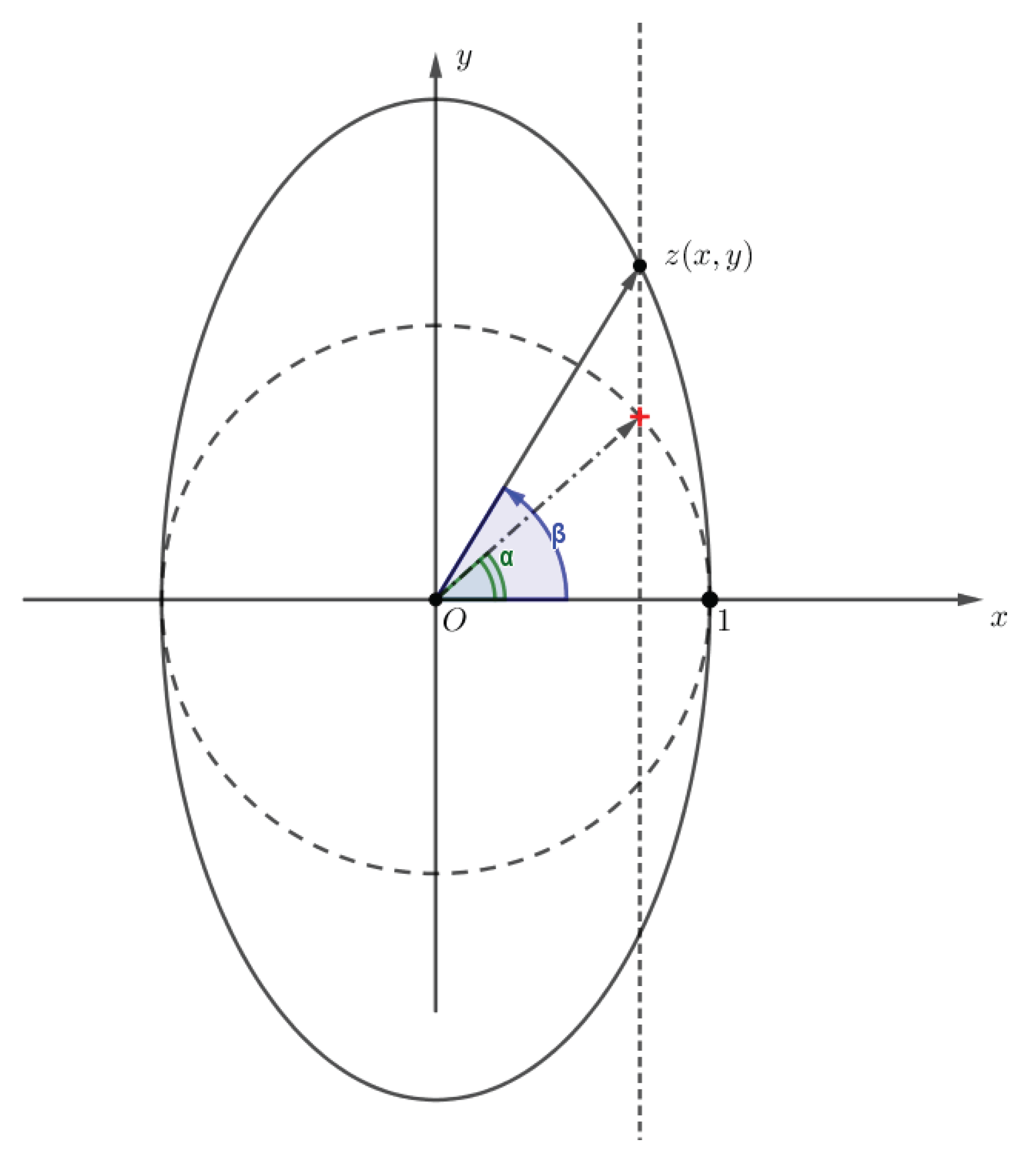
Figure 2.
The geometric significance of the complex plane ()
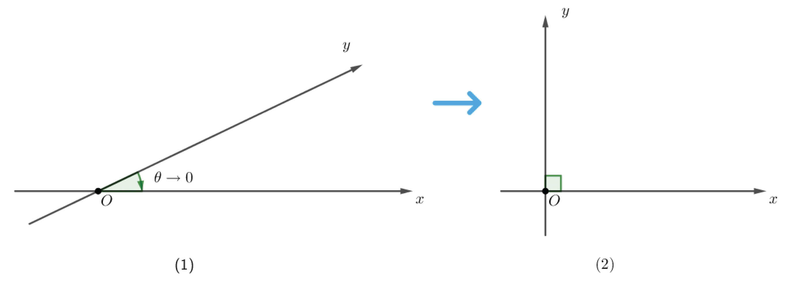
Figure 3.
The geometric significance of the complex plane ()
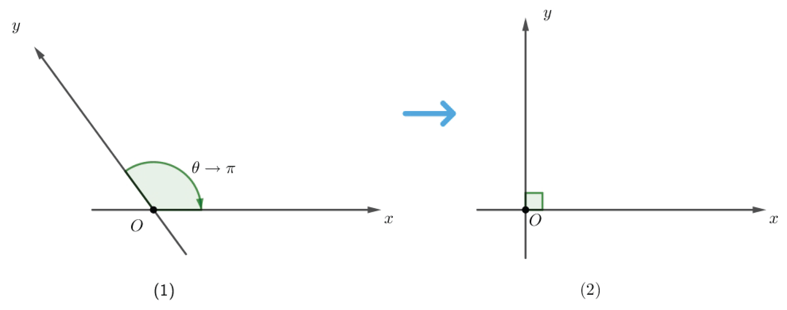
Figure 4.
The closed curve in the complex plane where .
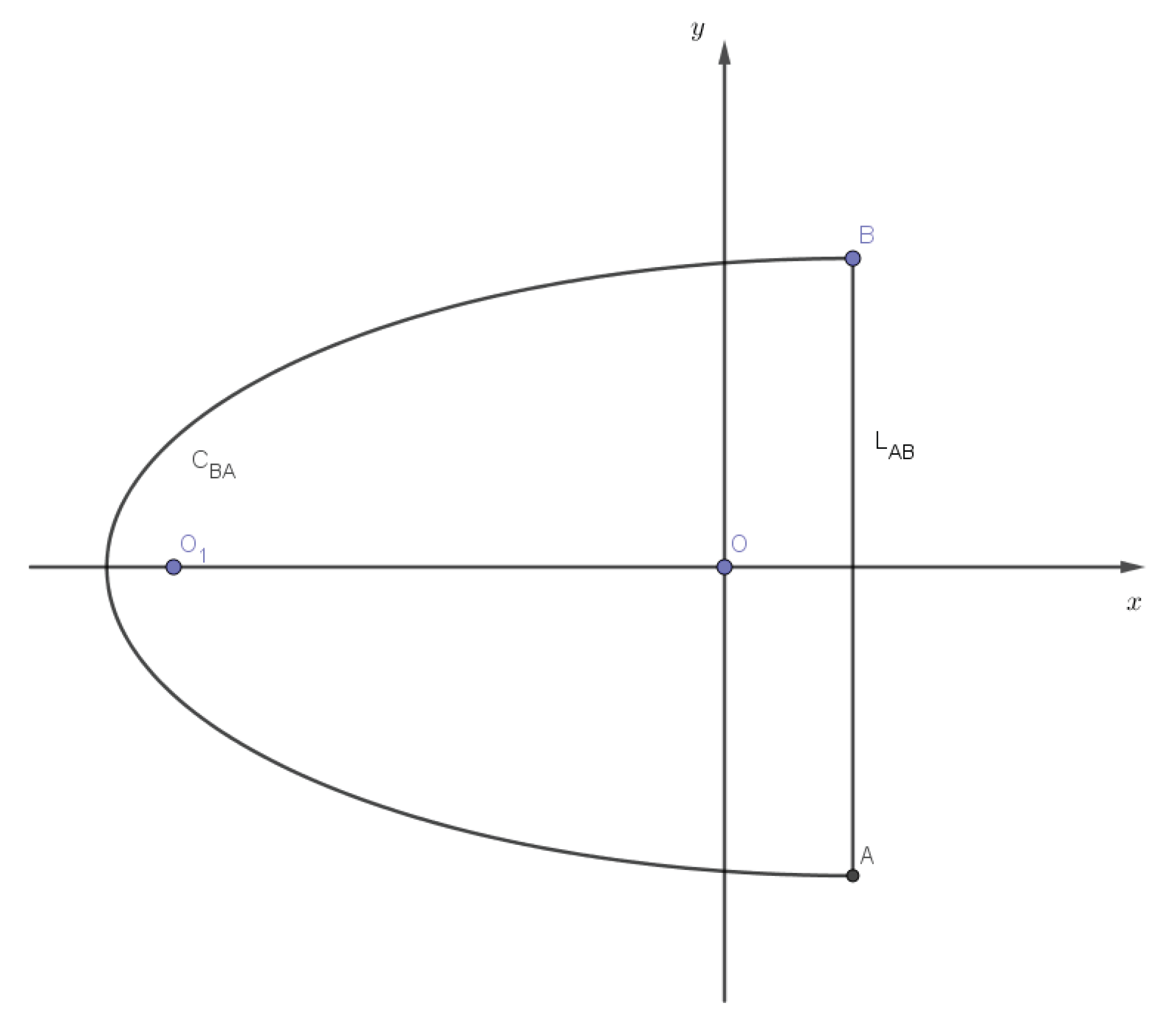
Figure 5.
The contour employed for the function in the complex plane .
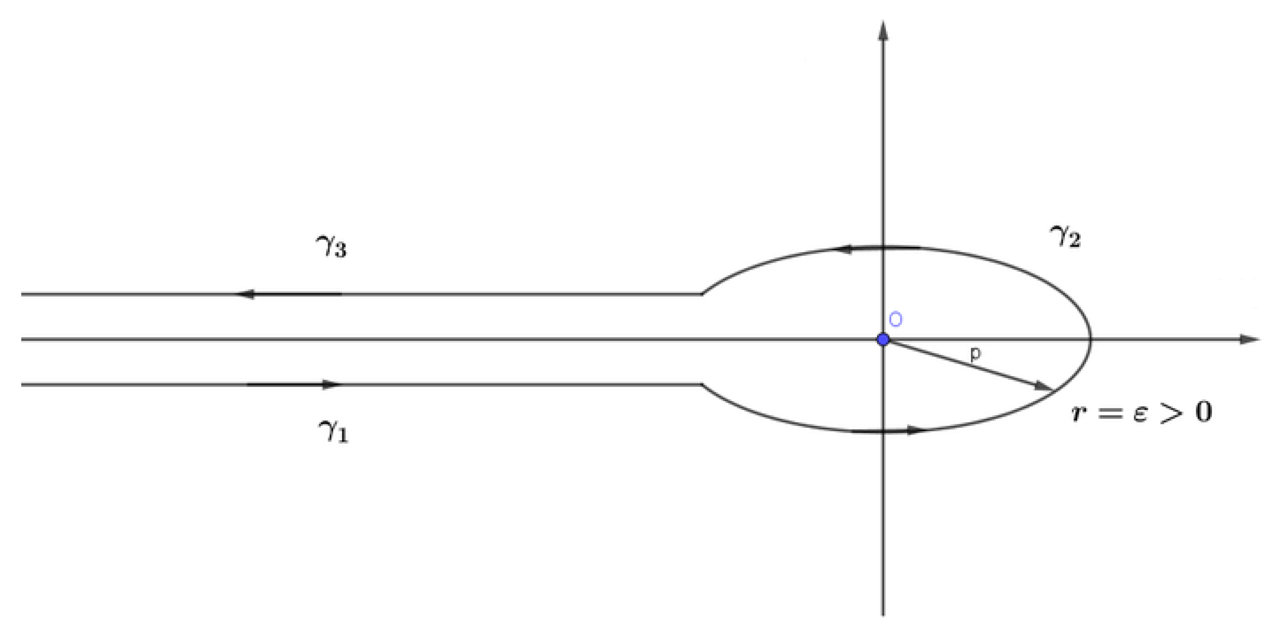
Figure 6.
The contour employed for the function in the complex plane .
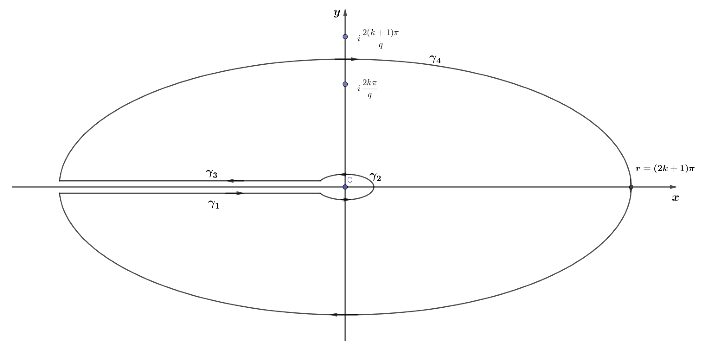
Figure 7.
The correspondence of zeros of between elliptic complex planes.
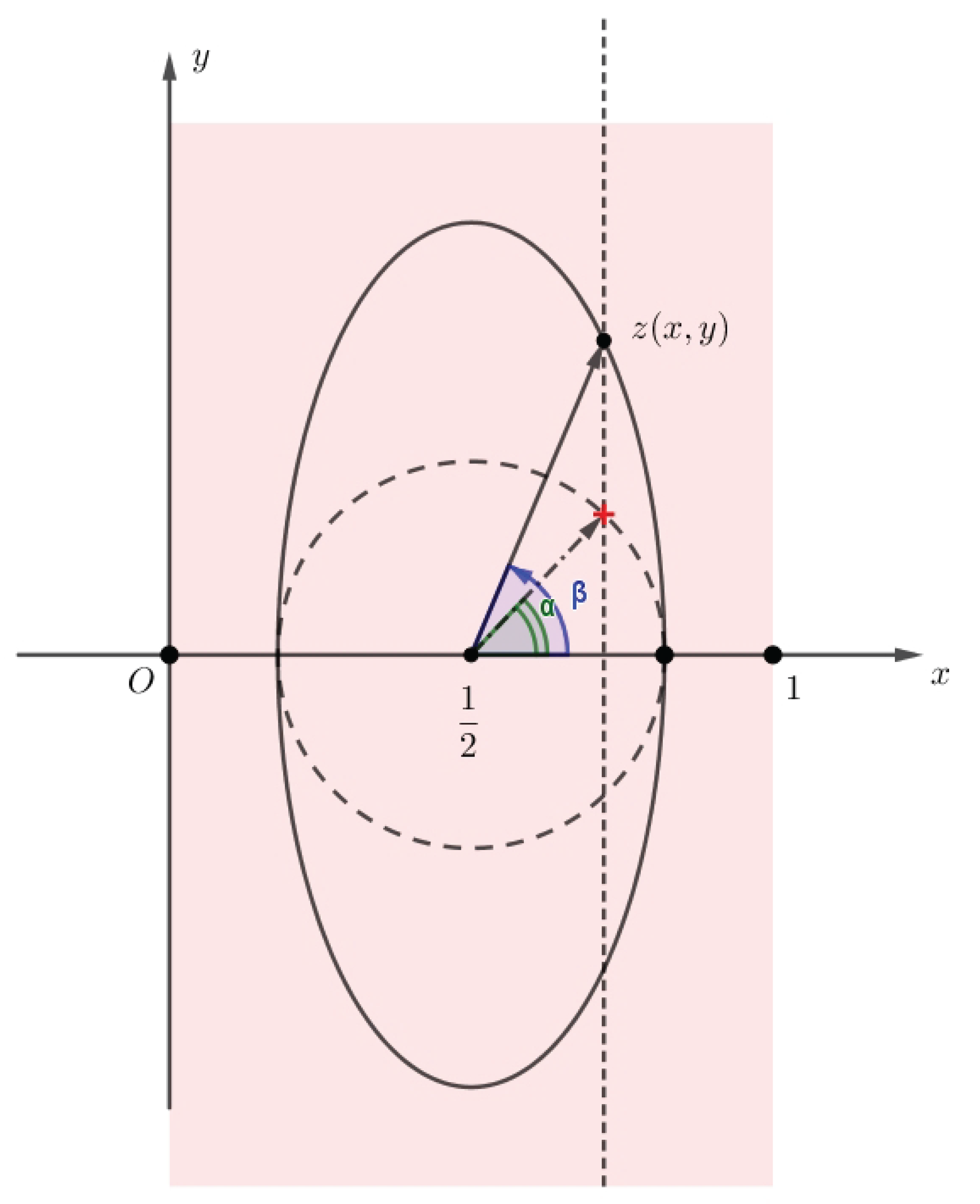
Disclaimer/Publisher’s Note: The statements, opinions and data contained in all publications are solely those of the individual author(s) and contributor(s) and not of MDPI and/or the editor(s). MDPI and/or the editor(s) disclaim responsibility for any injury to people or property resulting from any ideas, methods, instructions or products referred to in the content. |
© 2026 by the authors. Licensee MDPI, Basel, Switzerland. This article is an open access article distributed under the terms and conditions of the Creative Commons Attribution (CC BY) license (http://creativecommons.org/licenses/by/4.0/).
Copyright: This open access article is published under a Creative Commons CC BY 4.0 license, which permit the free download, distribution, and reuse, provided that the author and preprint are cited in any reuse.