Homotopy Groups of Spheres, Hopf Fibrations and Villarceau Circles II Advances in Fiber Bundle Topology and Spherical Homotopy Theory

1. Introduction

The study of spheres is a cornerstone of topology. While in geometry we are concerned with exact distances and curvature, topology treats spheres as fundamental shapes that can be stretched and deformed. The central question of homotopy theory is: How can one sphere be continuously deformed into another? More formally, we study the set of continuous maps from one sphere to another, up to continuous deformation, or homotopy. These sets form groups, known as the homotopy groups of spheres, denoted ${\pi }_n\left(S^k\right)$.1

At first glance, one might think that ${\pi }_n\left(S^k\right)$ is trivial for $n<k$, as it seems impossible to wrap a smaller sphere around a larger one in an essential way. This is indeed true: ${\pi }_n\left(S^k\right)=0$ for $n<k$.2 The first non-trivial case appears when $n=k$, where ${\pi }_k\left(S^k\right)\cong \mathbb{Z}$, classified by the degree of the map.3 The true complexity and beauty of the subject emerge when $n>k$. For instance, ${\pi }_3\left(S^2\right)\cong \mathbb{Z}$, a result that is not at all obvious from a geometric standpoint. How can a 3-sphere wrap around a 2-sphere in an infinite number of essentially different ways? The answer lies in the Hopf fibration.

This paper aims to demystify these concepts. We will start with the fundamentals of homotopy theory, then delve into the theory of fibrations, with a laser focus on the Hopf fibrations. We will show how the Hopf map $h:S^3\to S^2$ serves as the generator of ${\pi }_3\left(S^2\right)$. Finally, we will uncover the surprising link to Villarceau circles, showing that the fibers of the Hopf map are not just abstract circles, but are precisely the Villarceau circles that lie on nested tori filling $S^3$. This connection provides a tangible geometric visualization of a deep topological fact.

The subject of homotopy groups of spheres has a rich history, from the early work of Brouwer and Hopf to the modern era of stable homotopy theory and chromatic methods. The calculation of these groups remains one of the most challenging and fundamental problems in algebraic topology. In this expanded exposition, we aim to provide a thorough grounding in the classical results while also pointing toward contemporary developments. We will discuss the Freudenthal suspension theorem, the stable homotopy groups, the Hopf invariant one problem solved by Adams, and the recent connections to Calabi-Yau manifolds and mirror symmetry. Throughout, we emphasize the interplay between algebraic and geometric methods.

The structure of the paper is as follows. Section 2 covers the foundational concepts of homotopy, homotopy equivalence, and the basic properties of homotopy groups. Section 3 introduces fibrations and the long exact sequence, with many examples. Section 4 is devoted entirely to the Hopf fibrations, including the real, complex, quaternionic, and octonionic cases, and their role in computing homotopy groups. Section 5 explores the beautiful geometry of Villarceau circles and their relation to the Hopf fibration. Section 6 discusses stable homotopy theory and the known calculations. Section 7 outlines recent generalizations to Calabi-Yau manifolds and the SYZ conjecture. Finally, Section 8 concludes with open problems and future directions. Several appendices provide detailed proofs, tables of homotopy groups, and algorithmic approaches to computations.

2. Foundations of Homotopy Theory

To understand the homotopy groups of spheres, we must first establish the formal language of homotopy theory. This section provides the necessary definitions and foundational theorems, accompanied by numerous examples and exercises.

2.1. Homotopy and Homotopy Equivalence

Definition 2.1 

(Homotopy). Let $f,g:X\to Y$ be continuous maps between topological spaces. A homotopy from f to g is a continuous map

$$H:X\times [0,1]\to Y$$

such that $H(x,0)=f\left(x\right)$ and $H(x,1)=g\left(x\right)$ for all $x\in X$. If such a homotopy exists, we say f is homotopic to g, and write $f\simeq g$.4

Definition 2.2 

(Homotopy Equivalence). Two spaces X and Y are homotopy equivalent, or have the same homotopy type, if there exist continuous maps $f:X\to Y$ and $g:Y\to X$ such that $g\circ f\simeq$ and $f\circ g\simeq$ . The maps f and g are called homotopy equivalences.5

Example 2.3 

(Contractible Spaces). A space that is homotopy equivalent to a point is called contractible. For instance, ${\mathbb{R}}^n$ is contractible: the map $H(x,t)=(1-t)x$ gives a homotopy from the identity to the constant map at the origin. Similarly, any convex subset of ${\mathbb{R}}^n$ is contractible.

Example 2.4 

(Homotopy Equivalence of $S^1$ and ${\mathbb{R}}^2\setminus \left\{0\right\}$). The circle $S^1$ and the punctured plane ${\mathbb{R}}^2\setminus \left\{0\right\}$ are homotopy equivalent. Define $f:S^1\hookrightarrow {\mathbb{R}}^2\setminus \left\{0\right\}$ as inclusion, and $g:{\mathbb{R}}^2\setminus \left\{0\right\}\to S^1$ by $g\left(x\right)=x/\left|x\right|$. Then $g\circ f={id}_{S^1}$, and $f\circ g$ is homotopic to the identity via $H(x,t)=(1-t)x+tx/\left|x\right|$. This homotopy is well-defined because the line segment from x to its unit normalization never passes through the origin.

Definition 2.5 

(Relative Homotopy). Let $A\subset X$ be a subspace. Two maps $f,g:X\to Y$ are homotopic relative to A if there is a homotopy $H:X\times I\to Y$ such that $H(a,t)=f\left(a\right)=g\left(a\right)$ for all $a\in A$ and all $t\in I$. We write $f\simeq g\mathrm{rel}A$.

2.2. Cell Complexes and CW Approximation

Many spaces of interest, including spheres, can be built by attaching cells. This structure is captured by the notion of a CW complex, introduced by J. H. C. Whitehead. CW complexes are particularly convenient for homotopy theory because of the cellular approximation theorem.

Definition 2.6 

(CW Complex). A CW complex is a topological space X equipped with a filtration

$$X^0\subset X^1\subset X^2\subset \cdots \subset X$$

such that:

• $X^0$ is a discrete set of points (0-cells).
• For each $n\ge 1$, $X^n$ is obtained from $X^{n-1}$ by attaching n-cells $e_{\alpha }^n$ via attaching maps ${\phi }_{\alpha }:S^{n-1}\to X^{n-1}$.
• The topology on X is the weak topology: a set is closed iff its intersection with each $X^n$ is closed.
• X has the closure-finite condition: each cell meets only finitely many other cells.

Spheres have a natural CW structure: $S^n$ can be built from one 0-cell and one n-cell, with the attaching map collapsing the boundary of the n-disk to the point.

Theorem 2.7 

(Cellular Approximation Theorem). Every continuous map $f:X\to Y$ between CW complexes is homotopic to a cellular map, i.e., a map satisfying $f\left(X^n\right)\subset Y^n$ for all n. Moreover, if f is already cellular on a subcomplex, the homotopy can be chosen to be stationary on that subcomplex.

For a proof, see ([1] Theorem 4.8). This theorem is instrumental in proving many basic results about homotopy groups.

2.3. Homotopy Groups

Homotopy groups are higher-dimensional analogs of the fundamental group. They capture information about the number of “holes” in a space in each dimension.

Definition 2.8 

(Homotopy Group). Let X be a topological space with a chosen basepoint $x_0\in X$. Consider the set of continuous maps $f:(I^n,\partial I^n)\to (X,x_0)$, where $I^n$ is the n-dimensional cube and $\partial I^n$ is its boundary. Two such maps are considered equivalent if they are homotopic through maps that keep the boundary fixed at $x_0$. The set of equivalence classes, denoted ${\pi }_n(X,x_0)$, forms a group under concatenation of maps. For $n\ge 1$, this is the n-th homotopy group. For $n=1$, this is the fundamental group.6

Remark 2.9. 

For path-connected spaces, the homotopy groups are independent of the basepoint up to isomorphism, so we often write ${\pi }_n\left(X\right)$.

Example 2.10. 

• ${\pi }_n\left(\mathrm{point}\right)=0$ for all n.
• ${\pi }_1\left(S^1\right)\cong \mathbb{Z}$, ${\pi }_n\left(S^1\right)=0$ for $n>1$ because the universal cover $\mathbb{R}$ is contractible.
• ${\pi }_n\left(S^n\right)\cong \mathbb{Z}$, generated by the identity map.
• ${\pi }_3\left(S^2\right)\cong \mathbb{Z}$, as we will see via the Hopf fibration.

2.4. First Calculations and the Freudenthal Suspension Theorem

The very first calculations are straightforward for $n\le k$.

Theorem 2.11. 

For $n<k$, ${\pi }_n\left(S^k\right)=0$. For $n=k$, ${\pi }_k\left(S^k\right)\cong \mathbb{Z}$.7

The case $n>k$ is far more intricate. A fundamental tool for understanding the relationship between homotopy groups in different dimensions is the Freudenthal suspension theorem.

Definition 2.12 

(Suspension). The (reduced) suspension $\Sigma X$ of a pointed space $(X,x_0)$ is the quotient

$$\Sigma X=(X\times I)/(X\times \left\{0\right\}\cup X\times \left\{1\right\}\cup \left\{x_0\right\}\times I).$$

For a sphere, $\Sigma S^n\cong S^{n+1}$. Given a map $f:X\to Y$, the suspension $\Sigma f:\Sigma X\to \Sigma Y$ is defined by $(\Sigma f)\left(\right[x,t\left]\right)=\left[f\right(x),t]$.

Theorem 2.13 

(Freudenthal Suspension Theorem). The suspension homomorphism $E:{\pi }_n\left(S^k\right)\to {\pi }_{n+1}\left(S^{k+1}\right)$ is an isomorphism for $n<2k-1$ and a surjection for $n=2k-1$.8

The Freudenthal theorem is proved using CW approximation and the fact that the suspension map induces an isomorphism in a certain range. It implies that for fixed n, the groups ${\pi }_{n+k}\left(S^k\right)$ eventually become constant as k increases. This stable value is denoted ${\pi }_n^s$, the n-th stable homotopy group of spheres.

Table 1. Some low-dimensional homotopy groups of spheres (source: [11])

$\mathit{k}\setminus \mathit{n}$	1	2	3	4	5	6
1	$\mathbb{Z}$	0	0	0	0	0
2	0	$\mathbb{Z}$	$\mathbb{Z}$	${\mathbb{Z}}_2$	${\mathbb{Z}}_2$	${\mathbb{Z}}_{12}$
3	0	0	$\mathbb{Z}$	${\mathbb{Z}}_2$	${\mathbb{Z}}_2$	${\mathbb{Z}}_{12}$
4	0	0	0	$\mathbb{Z}$	${\mathbb{Z}}_2$	${\mathbb{Z}}_2$
5	0	0	0	0	$\mathbb{Z}$	${\mathbb{Z}}_2$
6	0	0	0	0	0	$\mathbb{Z}$

Table 1. Some low-dimensional homotopy groups of spheres (source: [11])

$\mathit{k}\setminus \mathit{n}$	1	2	3	4	5	6
1	$\mathbb{Z}$	0	0	0	0	0
2	0	$\mathbb{Z}$	$\mathbb{Z}$	${\mathbb{Z}}_2$	${\mathbb{Z}}_2$	${\mathbb{Z}}_{12}$
3	0	0	$\mathbb{Z}$	${\mathbb{Z}}_2$	${\mathbb{Z}}_2$	${\mathbb{Z}}_{12}$
4	0	0	0	$\mathbb{Z}$	${\mathbb{Z}}_2$	${\mathbb{Z}}_2$
5	0	0	0	0	$\mathbb{Z}$	${\mathbb{Z}}_2$
6	0	0	0	0	0	$\mathbb{Z}$

2.5. Relative Homotopy Groups and Exact Sequences

For a pair $(X,A)$ with basepoint $x_0\in A$, one defines relative homotopy groups ${\pi }_n(X,A,x_0)$ consisting of homotopy classes of maps $(D^n,S^{n-1},s_0)\to (X,A,x_0)$. There is a long exact sequence:

$$\cdots \to {\pi }_n\left(A\right)\to {\pi }_n\left(X\right)\to {\pi }_n(X,A)\to {\pi }_{n-1}\left(A\right)\to \cdots \to {\pi }_0\left(X\right).$$

This sequence is a fundamental tool for computations. For a fibration, a similar long exact sequence exists, which we will explore in the next section.

3. Fibrations and Covering Spaces

To compute higher homotopy groups, we need tools that relate the homotopy groups of different spaces. Fibrations are one such tool, acting as a topological version of a projection map with a “homotopy lifting property.”

3.1. Definition and Homotopy Lifting Property

Definition 3.1 

(Fibration). A continuous map $p:E\to B$ has the homotopy lifting property with respect to a space X if for every homotopy $f_t:X\to B$ and a lift ${\tilde{f}}_0:X\to E$ of $f_0$ (i.e., $p\circ {\tilde{f}}_0=f_0$), there exists a homotopy ${\tilde{f}}_t:X\to E$ lifting $f_t$ (i.e., $p\circ {\tilde{f}}_t=f_t$). A map $p:E\to B$ is a fibration (or Hurewicz fibration) if it has the homotopy lifting property with respect to all spaces X. A Serre fibration has this property for all cubes $X=I^n$.9

Example 3.2 

(Product Fibrations). The projection $p:B\times F\to B$ is a fibration (in fact a trivial fiber bundle). The fiber is F. Lifting a homotopy is simply given by ${\tilde{f}}_t\left(x\right)=(f_t\left(x\right),{\tilde{f}}_0{\left(x\right)}_F)$ where ${\tilde{f}}_0{\left(x\right)}_F$ is the F-component of the initial lift.

Example 3.3 

(Covering Spaces). A covering space $p:\tilde{X}\to X$ is a fibration with discrete fiber. The homotopy lifting property holds uniquely; this is the classical path-lifting property.

Example 3.4 

(Hopf Fibrations). The Hopf maps $S^3\to S^2$, $S^7\to S^4$, $S^{15}\to S^8$ are fibrations with fibers $S^1,S^3,S^7$ respectively. They are not product fibrations; they are nontrivial fiber bundles.

3.2. The Long Exact Sequence of a Fibration

The primary utility of a fibration $F\hookrightarrow E\stackrel{p}{\to }B$ is the long exact sequence of homotopy groups it induces.

Theorem 3.5 

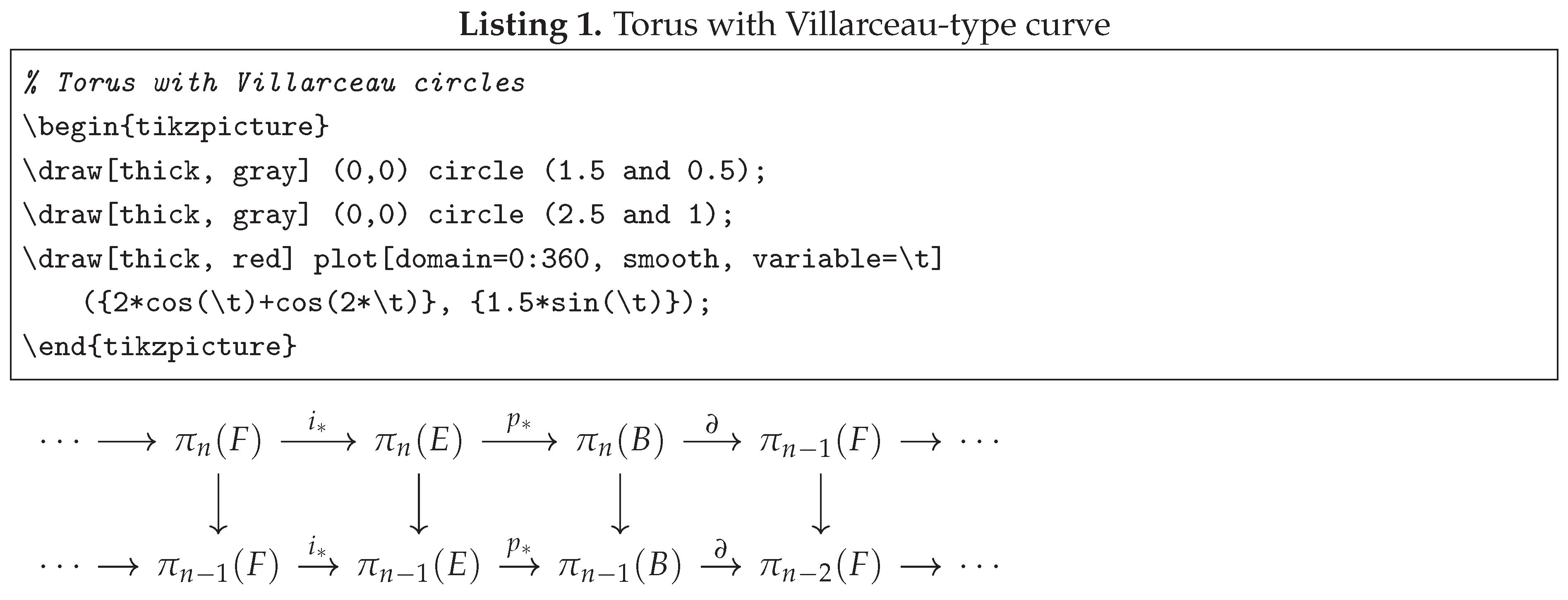
(Long Exact Sequence of a Fibration). For a Serre fibration $p:E\to B$ with fiber $F=p^{-1}\left(b_0\right)$, there is a long exact sequence of homotopy groups:

$$\cdots \to {\pi }_n\left(F\right)\stackrel{i_{*}}{\to }{\pi }_n\left(E\right)\stackrel{p_{*}}{\to }{\pi }_n\left(B\right)\stackrel{\partial }{\to }{\pi }_{n-1}\left(F\right)\to \cdots \to {\pi }_0\left(E\right)\to {\pi }_0\left(B\right)$$

where $i:F\hookrightarrow E$ is the inclusion, and ∂ is the connecting homomorphism.10

The proof uses the homotopy lifting property to construct the boundary map and exactness is verified by standard diagram chasing. A detailed proof can be found in ([1] Section 4.2).

Example 3.6 

(Hopf fibration $S^1\to S^3\to S^2$). Applying the long exact sequence:

$$\cdots \to {\pi }_3\left(S^1\right)\to {\pi }_3\left(S^3\right)\to {\pi }_3\left(S^2\right)\to {\pi }_2\left(S^1\right)\to {\pi }_2\left(S^3\right)\to \cdots$$

We know ${\pi }_n\left(S^1\right)=0$ for $n>1$ and ${\pi }_3\left(S^3\right)\cong \mathbb{Z}$. Also ${\pi }_2\left(S^3\right)=0$. Thus we get:

$$0\to \mathbb{Z}\to {\pi }_3\left(S^2\right)\to 0,$$

so ${\pi }_3\left(S^2\right)\cong \mathbb{Z}$. The generator is the homotopy class of the Hopf map itself.

Example 3.7 

(Hopf fibration $S^3\to S^7\to S^4$). The long exact sequence gives:

$$\cdots \to {\pi }_7\left(S^3\right)\to {\pi }_7\left(S^7\right)\to {\pi }_7\left(S^4\right)\to {\pi }_6\left(S^3\right)\to \cdots$$

Using known facts: ${\pi }_7\left(S^7\right)\cong \mathbb{Z}$, ${\pi }_7\left(S^3\right)\cong {\mathbb{Z}}_2$ (this is a deep result), and ${\pi }_6\left(S^3\right)\cong {\mathbb{Z}}_{12}$. The sequence helps compute ${\pi }_7\left(S^4\right)$; it turns out to be $\mathbb{Z}\oplus {\mathbb{Z}}_{12}$. This is a nontrivial calculation that illustrates the power of the long exact sequence.

3.3. More Examples of Fibrations

• Path-loop fibration: For any space X with basepoint, the evaluation map $\mathrm{ev}:PX\to X$ from the space of paths starting at the basepoint is a fibration with fiber the loop space $\mathsf{\Omega }X$. The long exact sequence gives a relationship between homotopy groups of X and loop spaces: ${\pi }_n\left(\mathsf{\Omega }X\right)\cong {\pi }_{n+1}\left(X\right)$.
• Sphere bundles: The tangent sphere bundle of a manifold is a fibration. For $S^2$, the unit tangent bundle is $SO\left(3\right)\cong \mathbb{R}{P}^3$, giving a fibration $S^1\to S^3\to S^2$ again.
• Principal bundles: Given a topological group G and a principal G-bundle $G\to E\to B$, the long exact sequence relates homotopy groups of G, E, and B.

4. The Hopf Fibrations

The Hopf fibrations are a family of four remarkable fibrations of spheres by spheres. They are the only such fibrations and are deeply connected to the real numbers, complex numbers, quaternions, and octonions.

4.1. The Complex Hopf Fibration: $S^1\hookrightarrow S^3\to S^2$

This is the most famous and the one most relevant to this paper.

Definition 4.1 

(Hopf Map). Consider $S^3$ as the set of points in ${\mathbb{C}}^2$ with $|z_1{|}^2+{\left|z_2\right|}^2=1$, and $S^2$ as the complex projective line ${\mathbb{CP}}^1$, which is the set of complex lines through the origin in ${\mathbb{C}}^2$. The Hopf map $h:S^3\to S^2$ is defined by

$$h(z_1,z_2)=[z_1:z_2]\in {\mathbb{CP}}^1.$$

In terms of coordinates on $S^2\cong \mathbb{C}\cup \{\infty \}$, this is often written as $h(z_1,z_2)=z_1/z_2$, interpreting the result as a point on the Riemann sphere.11

Theorem 4.2. 

The Hopf map $h:S^3\to S^2$ is the generator of ${\pi }_3\left(S^2\right)\cong \mathbb{Z}$.12

4.2. The Quaternionic Hopf Fibration: $S^3\hookrightarrow S^7\to S^4$

Using quaternions $\mathbb{H}$, we define $S^7\subset {\mathbb{H}}^2$ as unit vectors. The Hopf map $h:S^7\to S^4$ is given by $h(q_1,q_2)=[q_1:q_2]\in {\mathbb{HP}}^1$, the quaternionic projective line, which is homeomorphic to $S^4$. The fibers are quaternionic lines, i.e., copies of $S^3$ (unit quaternions). This yields a fibration $S^3\to S^7\to S^4$.

Theorem 4.3. 

The quaternionic Hopf map generates a nontrivial element in ${\pi }_7\left(S^4\right)$. Using the long exact sequence, one can show that ${\pi }_7\left(S^4\right)\cong \mathbb{Z}\oplus {\mathbb{Z}}_{12}$, where the $\mathbb{Z}$ factor is generated by the Hopf map.

4.3. The Octonionic Hopf Fibration: $S^7\hookrightarrow S^{15}\to S^8$

Octonions $\mathbb{O}$ are non-associative, but one can still define a map $h:S^{15}\subset {\mathbb{O}}^2\to S^8$ by $h(o_1,o_2)=[o_1:o_2]$ with the understanding that projectivization requires care due to non-associativity. Nevertheless, this gives a fibration $S^7\to S^{15}\to S^8$ in the sense of a fiber bundle (though not a principal bundle because of non-associativity). It is still a Serre fibration.

Theorem 4.4 

(Adams’ Theorem on Hopf Invariant One). The only spheres that can support a Hopf fibration (i.e., a fiber bundle $S^a\to S^{2a+1}\to S^{a+1}$) occur for $a=1,3,7$. These correspond exactly to the real normed division algebras: $\mathbb{R}$, $\mathbb{C}$, $\mathbb{H}$, $\mathbb{O}$. Moreover, there is no such fibration for any other a because the Hopf invariant of such a map would be one, and Adams proved that elements of Hopf invariant one only exist in dimensions 1, 2, 4, 8 (i.e., for $a=1,3,7$). [3]

Table 2. The four Hopf fibrations

Fiber	Total space	Base space	Division algebra
$S^0$	$S^1$	$S^1$	$\mathbb{R}$
$S^1$	$S^3$	$S^2$	$\mathbb{C}$
$S^3$	$S^7$	$S^4$	$\mathbb{H}$
$S^7$	$S^{15}$	$S^8$	$\mathbb{O}$

Table 2. The four Hopf fibrations

Fiber	Total space	Base space	Division algebra
$S^0$	$S^1$	$S^1$	$\mathbb{R}$
$S^1$	$S^3$	$S^2$	$\mathbb{C}$
$S^3$	$S^7$	$S^4$	$\mathbb{H}$
$S^7$	$S^{15}$	$S^8$	$\mathbb{O}$

4.4. Linking and the Hopf Invariant

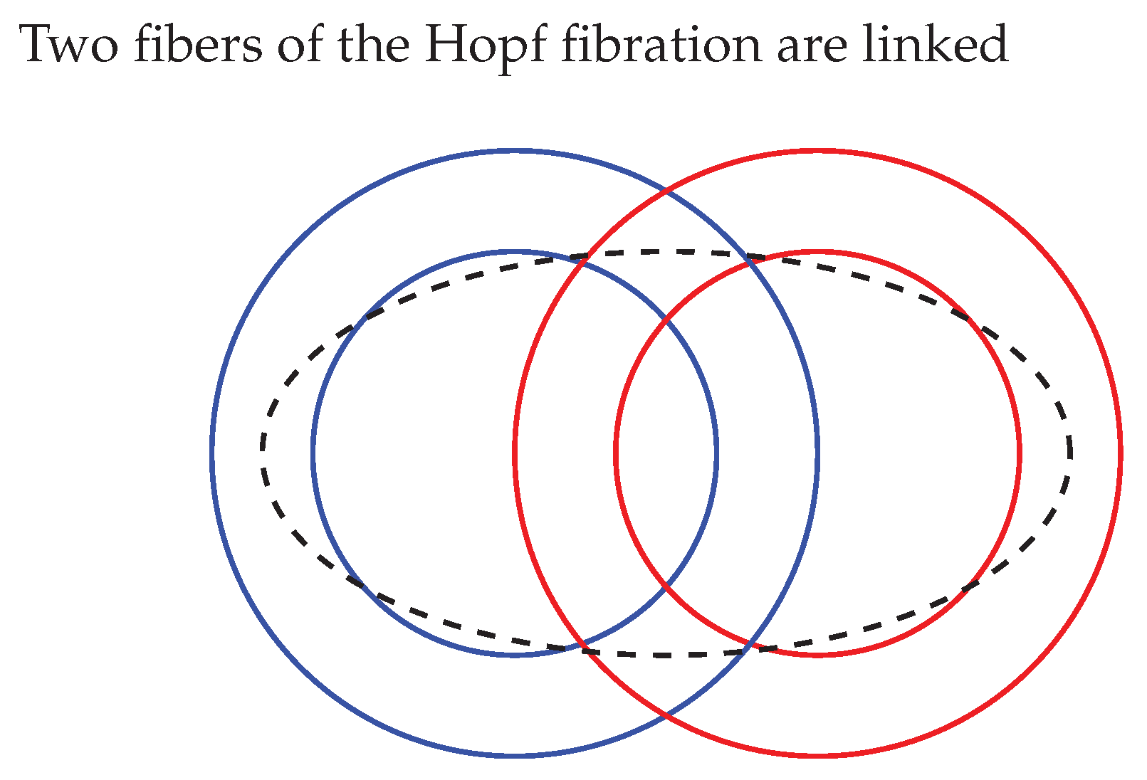
Given a map $f:S^{2n-1}\to S^n$, one can define the Hopf invariant $H\left(f\right)\in \mathbb{Z}$. For the Hopf maps, $H\left(f\right)=1$. The Hopf invariant is a homotopy invariant and is closely related to linking numbers of fibers. For the complex Hopf fibration, any two distinct fibers are linked with linking number 1. This geometric fact is a manifestation of the nontrivial Hopf invariant.

Figure 1. Schematic representation of linked circles (fibers) in $S^3$. In the actual 3-sphere, these circles are great circles and are linked exactly once.

Figure 1. Schematic representation of linked circles (fibers) in $S^3$. In the actual 3-sphere, these circles are great circles and are linked exactly once.

5. Villarceau Circles and the Hopf Fibration

The Hopf fibration is an abstract topological object, but it has a beautiful concrete geometric realization involving Villarceau circles on a torus.

5.1. Geometry of the Torus and Villarceau Circles

A torus is typically thought of as a surface of revolution. However, a torus also has a lesser-known set of circles, the Villarceau circles.

Definition 5.1 

(Villarceau Circles). Given a torus embedded in ${\mathbb{R}}^3$ or $S^3$, a Villarceau circle is a circle on the torus that is not a meridian (longitude) or a parallel (latitude). They are obtained by intersecting the torus with a plane that is tangent to it at two points. On any given torus, there are two such families of circles, each filling the torus.13

Parametrically, a torus in ${\mathbb{R}}^3$ can be given by

$$x=(R+rcos\theta )cos\varphi ,y=(R+rcos\theta )sin\varphi ,z=rsin\theta .$$

A Villarceau circle corresponds to a line of constant $\theta +\varphi$ (or $\theta -\varphi$) after an appropriate rotation. In terms of the two angles, a Villarceau circle is a curve where $\varphi$ and $\theta$ vary linearly with equal speed.

5.2. Linking and the Hopf Fibration

The connection to the Hopf fibration becomes clear when we consider the 3-sphere. The 3-sphere $S^3$ can be filled by nested tori. One common way to see this is through stereographic projection.

Theorem 5.2. 

The fibers of the Hopf fibration $h:S^3\to S^2$ are great circles. When $S^3$ is viewed as a union of nested tori (e.g., the preimages of circles of latitude on $S^2$), the Hopf fibers on each torus are precisely the Villarceau circles of that torus. Furthermore, any two distinct fibers are linked.14

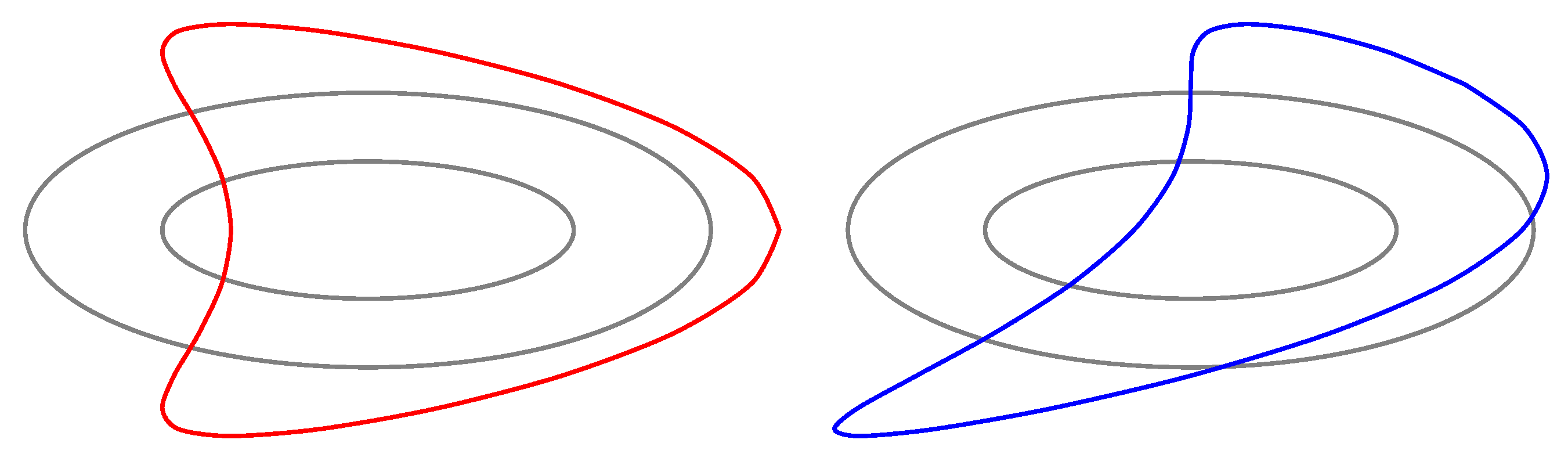
Figure 2. Two Villarceau circles on a torus. They wrap around both the meridian and longitude directions. In the Hopf fibration, each such circle is a fiber.

Figure 2. Two Villarceau circles on a torus. They wrap around both the meridian and longitude directions. In the Hopf fibration, each such circle is a fiber.

To see this explicitly, use coordinates on $S^3$:

$$S^3=\{(z,w)\in {\mathbb{C}}^2{:\left|z\right|}^2+{\left|w\right|}^2=1\}.$$

Let $T^2$ be the set where ${\left|z\right|}^2=a^2$, ${\left|w\right|}^2=b^2$ with $a^2+b^2=1$. This is a torus. The Hopf map sends $(z,w)$ to the ratio $z/w$. On this torus, the fibers are given by fixing the argument of $z/w$, i.e., $\arg z-\arg w=\mathrm{const}$. This is exactly a line of constant slope in the $(\arg z,\arg w)$ coordinates, which corresponds to a Villarceau circle. For an in-depth discussion, see [8].

5.3. Visualization with Stereographic Projection

Stereographic projection maps $S^3\setminus \left\{point\right\}$ to ${\mathbb{R}}^3$. Under this projection, the Hopf fibers become a family of linked circles in ${\mathbb{R}}^3$ that fill space. The nested tori become nested tori of revolution in ${\mathbb{R}}^3$. This classic visualization can be found in many online resources and is an excellent way to build intuition.

6. Stable Homotopy Groups and the Adams Conjecture

The Freudenthal suspension theorem tells us that for each n, the groups ${\pi }_{n+k}\left(S^k\right)$ stabilize as $k\to \infty$. The stable value is denoted ${\pi }_n^s$, the n-th stable homotopy group of spheres. These groups are of central importance in algebraic topology; they are the homotopy groups of the sphere spectrum, and they appear in many contexts (e.g., the framed cobordism theorem of Pontryagin and Thom).

6.1. Definition and Basic Properties

Definition 6.1 

(Stable Homotopy Groups). The n-th stable homotopy group of spheres is

$${\pi }_n^s=\underset{k\to \infty }{lim}{\pi }_{n+k}\left(S^k\right),$$

where the limit is taken with respect to the suspension homomorphisms.

The stable groups are finite for $n>0$ (by a theorem of Serre), and they exhibit a rich structure. They are also the coefficient groups for the Adams spectral sequence, which is a primary computational tool.

Table 3. Stable homotopy groups of spheres for $n\le 15$ (source: [12])

n	${\mathit{\pi }}_{\mathit{n}}^{\mathit{s}}$
0	$\mathbb{Z}$
1	${\mathbb{Z}}_2$
2	${\mathbb{Z}}_2$
3	${\mathbb{Z}}_{24}$
4	0
5	0
6	${\mathbb{Z}}_2$
7	${\mathbb{Z}}_{240}$
8	${\mathbb{Z}}_2\oplus {\mathbb{Z}}_2$
9	${\mathbb{Z}}_2\oplus {\mathbb{Z}}_2\oplus {\mathbb{Z}}_2$
10	${\mathbb{Z}}_6$
11	${\mathbb{Z}}_{504}$
12	0
13	${\mathbb{Z}}_3$
14	${\mathbb{Z}}_2$
15	${\mathbb{Z}}_{480}\oplus {\mathbb{Z}}_2$

Table 3. Stable homotopy groups of spheres for $n\le 15$ (source: [12])

n	${\mathit{\pi }}_{\mathit{n}}^{\mathit{s}}$
0	$\mathbb{Z}$
1	${\mathbb{Z}}_2$
2	${\mathbb{Z}}_2$
3	${\mathbb{Z}}_{24}$
4	0
5	0
6	${\mathbb{Z}}_2$
7	${\mathbb{Z}}_{240}$
8	${\mathbb{Z}}_2\oplus {\mathbb{Z}}_2$
9	${\mathbb{Z}}_2\oplus {\mathbb{Z}}_2\oplus {\mathbb{Z}}_2$
10	${\mathbb{Z}}_6$
11	${\mathbb{Z}}_{504}$
12	0
13	${\mathbb{Z}}_3$
14	${\mathbb{Z}}_2$
15	${\mathbb{Z}}_{480}\oplus {\mathbb{Z}}_2$

6.2. The Adams Spectral Sequence

The Adams spectral sequence is a powerful tool for computing stable homotopy groups. It takes the form

$$E_2^{s,t}={Ext}_{\mathcal{A}}^{s,t}(H^{*}(X;{\mathbb{Z}}_p),{\mathbb{Z}}_p)\Rightarrow {\pi }_{t-s}{\left(X\right)}_p^{\wedge },$$

where $\mathcal{A}$ is the mod p Steenrod algebra. For the sphere spectrum, this becomes a computation of the cohomology of the Steenrod algebra. The Adams spectral sequence has been completely worked out for many primes and dimensions, leading to the known stable groups.

Algorithm 1 Adams Spectral Sequence Computation (sketch)

1: Input: prime p, target dimension n 2: Compute the mod p cohomology of the sphere: $H^{*}(S^0;{\mathbb{Z}}_p)={\mathbb{Z}}_p$ in degree 0. 3: Compute the Steenrod algebra ${\mathcal{A}}_p$. 4: Compute ${Ext}_{{\mathcal{A}}_p}^{s,t}({\mathbb{Z}}_p,{\mathbb{Z}}_p)$ using a minimal resolution. 5: The $E_2$ page is given; differentials $d_r$ are determined by Massey products or by comparison with known groups. 6: After enough pages, the groups stabilize to the p-component of ${\pi }_n^s$. 7: Output the group.

The actual implementation of this algorithm is highly nontrivial and has been carried out by many researchers, culminating in the tables of Toda [11] and later by Ravenel [12].

6.3. The Adams Conjecture and Its Resolution

The Adams conjecture concerns the behavior of the J-homomorphism and the image of J in the stable homotopy groups. It was proved by Quillen and Sullivan in the 1970s. The J-homomorphism $J:{\pi }_n\left(SO\right)\to {\pi }_n^s$ maps from the homotopy groups of the stable orthogonal group to stable homotopy. The image of J is a cyclic summand in ${\pi }_n^s$ for certain n. The Adams conjecture states that the image of J is exactly the summand predicted by Adams in his work on the Hopf invariant one problem.

7. Generalizations and Recent Developments

The ideas of Hopf fibrations extend far beyond spheres. They are a special case of sphere bundles and have deep connections to various areas of mathematics and theoretical physics.

7.1. Hopf-like Fibrations on Calabi-Yau Manifolds

Recent work has explored the existence of fibrations with similar properties on more complex manifolds, such as Calabi-Yau manifolds. These manifolds are of central importance in string theory.

Remark 7.1. 

The structure of a Calabi-Yau manifold often allows for the construction of torus fibrations that are reminiscent of the Hopf fibration. These are known as special Lagrangian fibrations and are a key component of the SYZ conjecture in mirror symmetry. The fibers are special Lagrangian tori, and the base is a 3-sphere, mirroring the $S^3\to S^2$ structure in a higher-dimensional, more complex setting.15

The SYZ conjecture, proposed by Strominger, Yau, and Zaslow, asserts that a Calabi-Yau manifold should admit a special Lagrangian torus fibration over a 3-sphere, and mirror symmetry corresponds to T-duality on the fibers. This is a deep generalization of the Hopf fibration, where the fibers are now tori of dimension 3 (or higher) and the base is a sphere.

7.2. Other Generalizations

• Twistor fibrations: For oriented Riemannian 4-manifolds, the twistor space fibers over the manifold with fiber $S^2$. This is analogous to the Hopf fibration in the context of complex geometry.
• Quaternionic Hopf fibrations and instantons: The quaternionic Hopf map is related to the construction of instantons in Yang-Mills theory.
• Octonionic Hopf fibration and exceptional structures: The octonionic fibration appears in the context of the exceptional Lie groups and the classification of Riemannian holonomy.

8. Conclusion

The homotopy groups of spheres are a deep and intricate subject, sitting at the heart of algebraic topology. The Hopf fibrations provide a crucial bridge between abstract homotopy theory and concrete geometry. They not only allow for the computation of the first non-trivial higher homotopy group, ${\pi }_3\left(S^2\right)$, but also reveal a profound geometric structure within the 3-sphere itself.

The appearance of Villarceau circles as the fibers of this fibration is a beautiful example of how topology and geometry intertwine. It transforms the abstract notion of a homotopy class into a tangible picture of linked circles filling space. The legacy of these ideas continues to grow, finding new expressions in modern research on Calabi-Yau manifolds and mirror symmetry, proving that even classical results can illuminate the frontiers of science.

Future directions include a deeper understanding of the stable homotopy groups via chromatic homotopy theory, the exploration of higher-dimensional analogs in the context of M-theory, and the continued development of computational tools. The Hopf fibrations remain a source of inspiration and a testbed for new theories.

A.1.Proof of the Freudenthal Suspension Theorem (Sketch)

The theorem is proved using the notions of CW complexes and the homotopy excision theorem. For a detailed proof, see ([1] Chapter 4). The key idea is to consider the suspension map $E:{\pi }_n\left(S^k\right)\to {\pi }_{n+1}\left(S^{k+1}\right)$ and show that it is an isomorphism for $n<2k-1$ by constructing an inverse using the fact that the inclusion $S^k\hookrightarrow S^{k+1}$ is $(2k-1)$-connected.

A.2. Construction of the Connecting Homomorphism

For a fibration $F\to E\to B$, the connecting map $\partial :{\pi }_n\left(B\right)\to {\pi }_{n-1}\left(F\right)$ is defined as follows: represent an element of ${\pi }_n\left(B\right)$ by a map $f:I^n\to B$ sending $\partial I^n$ to the basepoint. Consider $I^n=I^{n-1}\times I$. Define a homotopy $f_t:I^{n-1}\to B$ by $f_t\left(x\right)=f(x,t)$. Lift this homotopy to ${\tilde{f}}_t:I^{n-1}\to E$ starting with a constant lift at the basepoint. Then ${\tilde{f}}_0$ maps $\partial I^{n-1}$ into the fiber, yielding an element of ${\pi }_{n-1}\left(F\right)$.

Table 4. Low-dimensional homotopy groups of spheres ${\pi }_{n+k}\left(S^k\right)$ for small $n,k$ (compiled from [11])

$k\setminus n$	1	2	3	4	5	6	7	8
1	$\mathbb{Z}$	0	0	0	0	0	0	0
2	0	$\mathbb{Z}$	$\mathbb{Z}$	${\mathbb{Z}}_2$	${\mathbb{Z}}_2$	${\mathbb{Z}}_{12}$	${\mathbb{Z}}_2$	${\mathbb{Z}}_2$
3	0	0	$\mathbb{Z}$	${\mathbb{Z}}_2$	${\mathbb{Z}}_2$	${\mathbb{Z}}_{12}$	${\mathbb{Z}}_2$	${\mathbb{Z}}_2$
4	0	0	0	$\mathbb{Z}$	${\mathbb{Z}}_2$	${\mathbb{Z}}_2$	${\mathbb{Z}}_{12}$	${\mathbb{Z}}_2$
5	0	0	0	0	$\mathbb{Z}$	${\mathbb{Z}}_2$	${\mathbb{Z}}_2$	${\mathbb{Z}}_{24}$
6	0	0	0	0	0	$\mathbb{Z}$	${\mathbb{Z}}_2$	${\mathbb{Z}}_2$
7	0	0	0	0	0	0	$\mathbb{Z}$	${\mathbb{Z}}_2$
8	0	0	0	0	0	0	0	$\mathbb{Z}$

Table 4. Low-dimensional homotopy groups of spheres ${\pi }_{n+k}\left(S^k\right)$ for small $n,k$ (compiled from [11])

$k\setminus n$	1	2	3	4	5	6	7	8
1	$\mathbb{Z}$	0	0	0	0	0	0	0
2	0	$\mathbb{Z}$	$\mathbb{Z}$	${\mathbb{Z}}_2$	${\mathbb{Z}}_2$	${\mathbb{Z}}_{12}$	${\mathbb{Z}}_2$	${\mathbb{Z}}_2$
3	0	0	$\mathbb{Z}$	${\mathbb{Z}}_2$	${\mathbb{Z}}_2$	${\mathbb{Z}}_{12}$	${\mathbb{Z}}_2$	${\mathbb{Z}}_2$
4	0	0	0	$\mathbb{Z}$	${\mathbb{Z}}_2$	${\mathbb{Z}}_2$	${\mathbb{Z}}_{12}$	${\mathbb{Z}}_2$
5	0	0	0	0	$\mathbb{Z}$	${\mathbb{Z}}_2$	${\mathbb{Z}}_2$	${\mathbb{Z}}_{24}$
6	0	0	0	0	0	$\mathbb{Z}$	${\mathbb{Z}}_2$	${\mathbb{Z}}_2$
7	0	0	0	0	0	0	$\mathbb{Z}$	${\mathbb{Z}}_2$
8	0	0	0	0	0	0	0	$\mathbb{Z}$

References

- A. Hatcher, Algebraic Topology. Cambridge University Press, 2002. [Link].
- R. Bott and L. W. Tu, Differential Forms in Algebraic Topology. Graduate Texts in Mathematics, vol. 82. Springer-Verlag, 1982. [Link].
- J. F. Adams, “On the non-existence of elements of Hopf invariant one,” Annals of Mathematics, vol. 72, no. 1, pp. 20-104, 1960. [JSTOR].
- D. Bhattacharjee, S. Singha Roy, and R. Sadhu, “Homotopy group of spheres, Hopf fibrations and Villarceau circles,” EPRA International Journal of Research & Development (IJRD), vol. 7, no. 9, September 2022. [CrossRef]
- D. Bhattacharjee and O. Frederick, “Hopf-Like Fibrations on Calabi-Yau Manifolds,” Preprints, 2025. [CrossRef]
- E. H. Spanier, Algebraic Topology. Springer-Verlag, 1981. [Link].
- G. W. Whitehead, Elements of Homotopy Theory. Graduate Texts in Mathematics, vol. 61. Springer-Verlag, 1978. [Link].
- D. W. Lyons, “An Elementary Introduction to the Hopf Fibration,” Mathematics Magazine, vol. 76, no. 2, pp. 87-98, 2003. [JSTOR].
- R. Penrose, The Road to Reality: A Complete Guide to the Laws of the Universe. Jonathan Cape, 2004. [Link].
- M. Nakahara, Geometry, Topology and Physics, 2nd ed. Institute of Physics Publishing, 2003. [Link].
- H. Toda, Composition Methods in Homotopy Groups of Spheres. Annals of Mathematics Studies, No. 49. Princeton University Press, 1962.
- D. C. Ravenel, Complex Cobordism and Stable Homotopy Groups of Spheres. Academic Press, 1986.
- J. P. May, A Concise Course in Algebraic Topology. University of Chicago Press, 1999.
- R. M. Switzer, Algebraic Topology — Homotopy and Homology. Springer-Verlag, 1975.
- A. Strominger, S.-T. Yau, and E. Zaslow, “Mirror symmetry is T-duality,” Nuclear Physics B, vol. 479, no. 1-2, pp. 243-259, 1996.
- M. F. Atiyah, “The Hopf fibration and the geometry of the octonions,” in Michael Atiyah: Collected Works, vol. 5, pp. 201-213, 1988.