Geometric Interpretation of Frequency Domain Robustness Constraints and Closed-Loop Pole Locations

1. Introduction

In several problems in control theory and applied mathematics, constraints on stability, robustness, and control performance are formulated as geometric sets in the complex plane [1,2,3,4,5]. In this context, the circle is used as a fundamental geometric object for describing admissible and forbidden regions arising from frequency-domain constraints, root-location conditions, and worst-case evaluations of the dynamic behavior of control systems [1,2,5]. The circle is not specific to a particular method of analysis or synthesis but results from the way engineering requirements for performance and robustness are formulated through modulus inequalities of complex functions [3,5].

The aim of the present study is to provide a geometric interpretation of a broad class of constraints used in control theory, by showing that they can be regarded as level sets of analytic and fractional-linear functions in the complex plane, without linear-matrix descriptions or optimization procedures. The study is carried out entirely at the level of description using the mathematical apparatus of transfer functions, which allows comparison of constraints in the frequency domain and constraints in the root plane and provides a geometric transition between them through preimages and images of circular sets.

Section 2 introduces the general mathematical formulation and formalizes the relationship between constraints on the modulus of a complex function in the frequency domain and the corresponding geometric sets in the complex plane. Section 3 derives the main geometric relationships that explain the invariance of circular constraints under fractional-linear transformations and their interpretation in the root plane. Section 4 proposes a geometric taxonomy of the main performance and robustness measures used in engineering practice, showing that gain margin, phase margin, and constraints on sensitivity and complementary sensitivity represent special cases of the same geometric mechanism. Section 5 presents a numerical example illustrating the practical applicability of the approach considered.

1.1. Related work

In the frequency domain, stability and robustness requirements are represented through constraints on the modulus of the frequency response of the open-loop system, which lead to circular admissible sets associated with gain margin, phase margin, sensitivity, and complementary sensitivity [6,7,8,9,10]. In the root plane, analogous geometric objects are used to define admissible regions for the locations of the closed-loop poles to guarantee desired dynamic behavior [11,12,13,14,15]. However, these geometric representations are usually considered as separate tools, depending on the specific analysis method, without emphasizing the common mechanism by which they arise [16,17,18].

The present review does not claim to provide exhaustive coverage of the entire literature in the field of robust control. It is based on established classical and contemporary directions that are directly related to the geometric interpretation of frequency domain constraints and their influence on the dynamics of closed-loop systems. The aim is to clarify the general geometric structure underlying these approaches, rather than to cover the full spectrum of existing methods.

More specifically, the reviewed literature includes classical robust control [[1[–[7], μ-analysis and methods for the analysis of structured uncertainty [[8[–[0], and H∞ approaches for analysis and synthesis in the frequency domain [1][–[3]. Contemporary frequency domain criteria for absolute stability and their geometric interpretation are summarized in [14], while the relationship between frequency domain constraints and modern analytical and numerical methods for robust analysis is discussed in detail in [15]. Probabilistic and randomized methods for robustness analysis are presented in [16,17,18,19,20].

In [21], robust tuning of classical controllers is analyzed through constraints on the sensitivity and complementary sensitivity functions interpreted in the Nyquist plane. In [22], the phase-root locus is introduced, providing a geometric link between stability margins in the frequency domain and root locations. In [23,24,25], disk margins and their associated geometric constraints in the Nyquist plane are considered. In [26], robust control is interpreted as a unifying geometric framework for classical frequency domain constraints, while in [27] a geometric analysis of admissible regions in the s- and z-complex planes for the assessment of stability and performance is proposed.

Despite the differences in methods and applications, these approaches do not formulate a common mechanism through which frequency domain constraints give rise to a specific geometric structure and relate to closed-loop pole locations.

Loop-shaping approaches allow the direct imposition of robustness and performance requirements through shaping of the frequency characteristics of the open loop in [28]. At the same time, as shown in [29], these methods are subject to fundamental trade-offs between stability, speed of response, and disturbance attenuation, which arise from intrinsic limitations of the feedback structure and cannot be eliminated by controller selection.

1.2. Motivation and Scope of the Proposed Approach

Despite the wide use of circular representations, frequency domain constraints related to various performance measures and robustness conditions are usually considered in isolation, depending on the specific analysis method or field of application. In the literature, they are introduced and interpreted separately as constraints related to the sensitivity function, the complementary sensitivity function, or geometric images of parametric uncertainty, without emphasizing the common geometric mechanism by which they arise [1,21,22,23,26,28].

At the same time, the dynamic properties of control systems are often analyzed in the s-plane, where admissible regions for closed-loop pole locations are introduced to guarantee desired closed-loop behavior.

In these approaches, the geometry of admissible regions in the s-plane plays a central role and is usually specified as a priori, without being derived directly from the constraints formulated in the frequency domain.

In [29], the constraints are considered at the level of fundamental trade-offs and informational limitations in feedback systems, while in [30,31,32,33] the geometry of stability regions is formalized through D-decomposition, geometrically oriented methods for root positioning, positive polynomials, and predefined admissible regions for the roots.

Following the classical results on root localization [29,30,31,32,33], more recent developments [34,35,36] consider geometric and analytical estimates relevant to robustness analysis. In these approaches, predefined admissible regions for closed-loop pole locations, linear-matrix conditions, or frequency criteria of the H∞, Bode, and singular value type are used for the assessment of stability and performance. However, the geometry of admissible regions is not derived directly from frequency domain constraints and is not formulated because of modulus inequalities in the Nyquist plane.

The analysis of the literature shows that a significant part of the scientific papers using geometric interpretations of frequency domain constraints were published around the beginning of the 2000s. This coincides with the period when classical frequency analysis and early robust control developed in parallel and a need arose for a geometric interpretation of new measures such as sensitivity, complementary sensitivity, and unified stability and performance margins. Subsequently, the focus of research shifted toward descriptions based on linear matrix inequalities and optimization and numerical methods, in which geometry remained in the background and was used mainly as an illustration rather than as an independent object of analysis, leaving the question “why do these constraints have precisely this geometric form” without a systematic answer.

For this reason, the present study returns to these questions and considers them again, using the contemporary language of level sets and fractional-linear transformations, in order to clarify the common mechanism by which the specified requirements in the frequency domain for robustness and performance give rise to circular sets and how these constraints are reflected in closed-loop pole locations in the s-plane.

In the present work, frequency domain constraints are represented as level sets of complex functions formulated directly through the mathematical apparatus of transfer functions. The approach makes it possible to investigate the geometric properties of these constraints and their reflection on closed-loop pole locations in the s-plane, without introducing a priori geometric regions.

On this basis, the main contribution of the study consists in clarifying the relationship between constraints on the modulus of complex functions in the frequency domain, the resulting circular sets, and the admissible or forbidden regions for closed-loop pole locations in the s-plane.

2. Mathematical Formulation

Let $s\in \mathbb{C}$ be a complex variable. The complex plane is considered in an abstract sense as the plane of the complex variable $s$, without prior specification of a particular physical interpretation. The specifications related to the frequency domain ($s=j\omega$) and to the s-plane are subsequently introduced as special cases of this general formulation. The complex variable $s$can be represented in the equivalent forms (1).

$$s=\sigma +j\omega ,s=r\left(\cos \phi +j\sin \phi \right),s=r{e}^{j\phi },$$

(1)

where $\sigma =Re(s)$, $\omega =\mathrm{I}m(s)$, $r=\left|s\right|$ и $\phi =\mathrm{a}\mathrm{r}\mathrm{g}(s)$.

Let $W(s)$ be a transfer function of a linear control system. Under the condition $\sigma =0$and $0\le \omega <\mathrm{\infty }$ and the substitution $s=j\omega$, the function $W\left(j\omega \right)$ describes the frequency response of the control system.

Assuming analytic continuation beyond the imaginary axis, i.e., $s=\sigma \pm j\omega$, the function $W(s)$ can be considered in the entire complex plane $\mathbb{C}$, which provides a connection between frequency properties and closed-loop pole locations of the system.

In control practice, a significant part of the constraints that guarantee robustness and performance are formulated in the frequency domain through conditions of the form (2).

$$\left|F\left(W\left(j\omega \right)\right)\right|\le c$$

(2)

where $F(\cdot )$ is an analytic or fractional-linear function, and $c>0$ is a real constant.

In the present work, two main classes of functions $F$are considered: fractional-linear (Möbius) transformations and more general analytic functions. For fractional-linear transformations, circular geometry is preserved both in the image and in the preimage, whereas for general analytic functions circular geometry arises at the level of the image but is not necessarily preserved in the preimage.

Constraints on the modulus of the functions $F(\cdot )$ have a clear geometric interpretation, as they define admissible regions in the complex plane $\mathbb{C}$, whose boundary has a circular form.

To provide a general description of these constraints, sets in the complex plane of the form (3) are considered.

$$C=\{W\in C: \left|F\left(W\right)\right|\le c\},$$

(3)

The boundary of the set $C$, defined by (3), is determined by the equality $\left|F\left(W\right)\right|=c$. When $F(\cdot )$ is a fractional-linear function, the set $C$has a strict boundary (a circle or a line in the degenerate case). For a general analytic function $F(\cdot )$, the circular geometry may be distorted, and the circular character is guaranteed only for fractional-linear transformations.

An essential property of such sets is their invariance under fractional-linear transformations of the form (4), under which the image and the preimage of a circle or a line are again a circle or a line.

$$F(W)={\displaystyle \frac{aW+b}{cW+d}},ad-bc\ne 0.$$

(4)

Therefore, for a fractional-linear function $F(\cdot )$, the boundary $\left|F\left(W\right)\right|=c$ preserves its circular character. This property explains the appearance of circular sets in the analysis of sensitivity, complementary sensitivity, and robustness constraints.

The relationship between frequency domain constraints and closed-loop pole locations can be formulated through the concept of the preimage of an admissible set. The set $S\subset \mathbb{C}$ will be called an admissible region in the s-plane, induced by the frequency domain constraint (2), and is defined as (5).

$$S=W^{-1}\left(C\right)=\left\{s\in \mathbb{C}:\left|F\left(W\left(s\right)\right)\right|\le c\right\},$$

(5)

where $W^{-1}(C)$ is the preimage of the set $C$ through the transfer function $W(s)$.

The boundary of the set $S$ in (5), denoted by $\partial S$, is obtained as the preimage of the circle $\left|F\left(W\right)\right|=c$. The resulting set $S\subset \mathbb{C}$ defines an admissible region in the plane of the complex variable $s$, induced by the frequency domain constraint (2).

In this way, the considered approach makes it possible to represent robustness constraints in the frequency domain as circular sets in the complex plane (for $s\to j\omega$), as well as to analyze their influence on closed-loop pole locations of the control system.

3. Geometric Dependencies and Unified Interpretation

In the following exposition, the complex function $W(s)$ is used as a generalized representation of various functions in control theory - open-loop or closed-loop transfer functions, the sensitivity function, and the complementary sensitivity function. Through the values of $W(s)$ in the complex plane, constraints on control performance are defined and considered in a geometric context.

In engineering practice, constraints on the dynamic behavior of systems are usually formulated through inequalities on the modulus of complex quantities. Regardless of the specific function, performance and robustness conditions most often take the form of modulus constraints of the type (2). The modulus has a clear engineering interpretation, as it represents gain in the worst-case sense and characterizes the influence of parametric or nonparametric disturbances on the system. For this reason, admissible sets in the complex plane naturally acquire a circular form, as shown in (3).

The geometric statements formulated below are a direct consequence of the mathematical formulation introduced in Section 2. They are based on the definition of the modulus level set (2), (3), on the invariance of generalized circles under fractional-linear transformations (4), and on the definition of the preimage of the admissible set in the complex s-plane (5). In this sense, no new theorems or proofs are introduced here; rather, the results of Section 2 are summarized in the context of control theory.

3.1. Geometric Statement (Modulus-Based Constraints and Circular Sets)

Constraints on control performance used in the analysis of performance and robustness of control systems are, in most cases, formulated through modulus inequalities of complex functions related to system dynamics. Conditions of the form (2), respectively their generalization in the complex s-plane defined by (5), define admissible sets in the complex plane whose boundary has circular geometry. Circular sets arise as a geometric consequence of the way real engineering requirements for performance and robustness are formulated in control theory, rather than as a priori introduced geometric objects.

3.2. Geometric Statement (Invariance of Circular Constraints under Fractional-Linear Transformations)

Circular sets defined through constraints on the modulus of the complex function $F(\cdot )$ preserve their geometric form under fractional-linear transformations of the complex plane. Under transformations of the form (4), the image of a circle or a union of circles is again a circle or a union of circles. More specifically, if the frequency domain constraint is given through the level set $C$, defined in (3) by the modulus inequality (2) with a fractional-linear function $F$ of the form (4), then any equivalent description obtained by composing $F$ with another fractional-linear function again leads to a set of the same type as $C$, i.e., with a circular (or, in the degenerate case, linear) boundary in the plane of $W(j\omega )$. This property explains why circular constraints appear in the analysis of different robustness measures in the frequency domain and provides a common geometric language for their description and comparison.

3.3. Geometric Statement (Interpretation of Frequency-Domain Constraints in the s-Plane)

Circular performance constraints formulated in the frequency domain through modulus inequalities (2) can be interpreted in the s-plane by considering the preimage of the admissible set. To the set $C$, given by (3), there corresponds the set $S$, given by (5), which defines an admissible region for the complex variable $s$. The resulting regions in the s-plane should be interpreted as a geometric reflection of robustness constraints in the frequency domain and allow analysis of dynamic properties arising from these constraints, without introducing new stability or performance criteria.

In particular, the requirement that all closed-loop poles belong to the set S represents a sufficient (but not necessary) condition that the frequency domain constraint (2), and therefore admissibility with respect to the set C, are satisfied for all considered frequencies.

3.4. Geometric Consequence (Unified Geometric Interpretation)

The three geometric relationships formulated in Geometric Statements 3.1–3.3 describe a common mechanism by which frequency domain constraints for performance and robustness are formulated as circular admissible sets in the complex plane of the function $W$ and are interpreted with respect to closed-loop pole locations of the system. The resulting regions should be regarded as a tool whose usefulness depends on the system dynamics and on the presence of dominant poles. Subsequently, this geometric framework is applied to specific classes of frequency domain constraints, showing how different performance and robustness measures in control theory arise as special cases of circular geometric constraints.

3.4. Engineering Interpretation of the Geometric Framework

The obtained geometric relationships show that a large part of the classical performance and robustness constraints in control theory arise because of modulus inequalities of complex functions. Circular sets are not a priori introduced geometric constructions, but a result of the way engineering requirements are formulated in the frequency domain. These modulus inequalities express constraints of the type “not to exceed a certain bound” and, in the context of robustness analysis, are interpreted as worst-case evaluations of sensitivity, complementary sensitivity, and the dynamic behavior of the system.

By defining the admissible set $C$ in the Nyquist plane and its preimage $S$ in the complex s-plane, robustness constraints obtain a simultaneous interpretation. In this sense, the geometric framework provides a common mechanism for comparing different performance measures, including constraints on sensitivity, complementary sensitivity, and classical stability margins.

The resulting regions in the s-plane should be regarded as a geometric reflection of the robustness constraints formulated in the frequency domain. In the presence of dominant poles, this relationship allows frequency domain requirements to be interpreted directly through closed-loop pole locations.

The considered approach does not introduce new stability criteria or design procedures, but serves as a geometric tool for interpreting, unifying, and comparing existing constraints in control theory. This geometric view is most transparent in the presence of dominant closed-loop poles.

4. Geometric Taxonomy of Circular Constraints in Control Theory

4.1. Circles Induced by Magnitude Constraints of Transfer Functions

Control performance constraints imposed on the modulus of the complex function $W(s)$, represented as the transfer function of an open-loop control system (6), are considered.

$$W(s)=C(s)P(s),$$

(6)

where $C(s)$ is the transfer function of the controller and $P(s)$ is the transfer function of the controlled process.

In this context, the complex functions (7) represent, respectively, the transfer function of the complementary sensitivity $T(s)$ and the transfer function of the sensitivity $S(s)$ of the closed-loop system (7).

$$T\left(s\right)={\displaystyle \frac{W\left(s\right)}{1+W\left(s\right)}}, S(s)={\displaystyle \frac{1}{1+W(s)}}$$

(7)

The function $T(s)$ describes the transfer from the input signal to the output of the system and is directly related to the dynamic properties and control performance of the closed-loop system. The function $S(s)$ characterizes the sensitivity of the closed-loop system to external disturbances and parametric uncertainty and is a fundamental measure in robust analysis of control systems.

According to Geometric Statement 3.1, constraints on the modulus of complex functions define circular admissible sets in the complex plane. In particular, the imposed frequency domain constraints for $s=j\omega$ of the form (8) define isomodular circles in the plane of the complex function $W$ (the open-loop system) and can be regarded not as separate cases, but as elements of the same class of geometric constraints, (8).

$$\left|W(j\omega )\right|=\mathrm{const},\left|T(j\omega )\right|=\mathrm{const},\left|S(j\omega )\right|=\mathrm{const}$$

(8)

Condition (9) defines a circle with center at the origin of the coordinate system and radius $\rho$in the complex plane of the open-loop system $W$, (9).

$$\left|W(j\omega )\right|=\rho$$

(9)

More interesting from the point of view of robustness and control performance are the constraints formulated through the transfer functions $S(s)$ and $T(s)$.

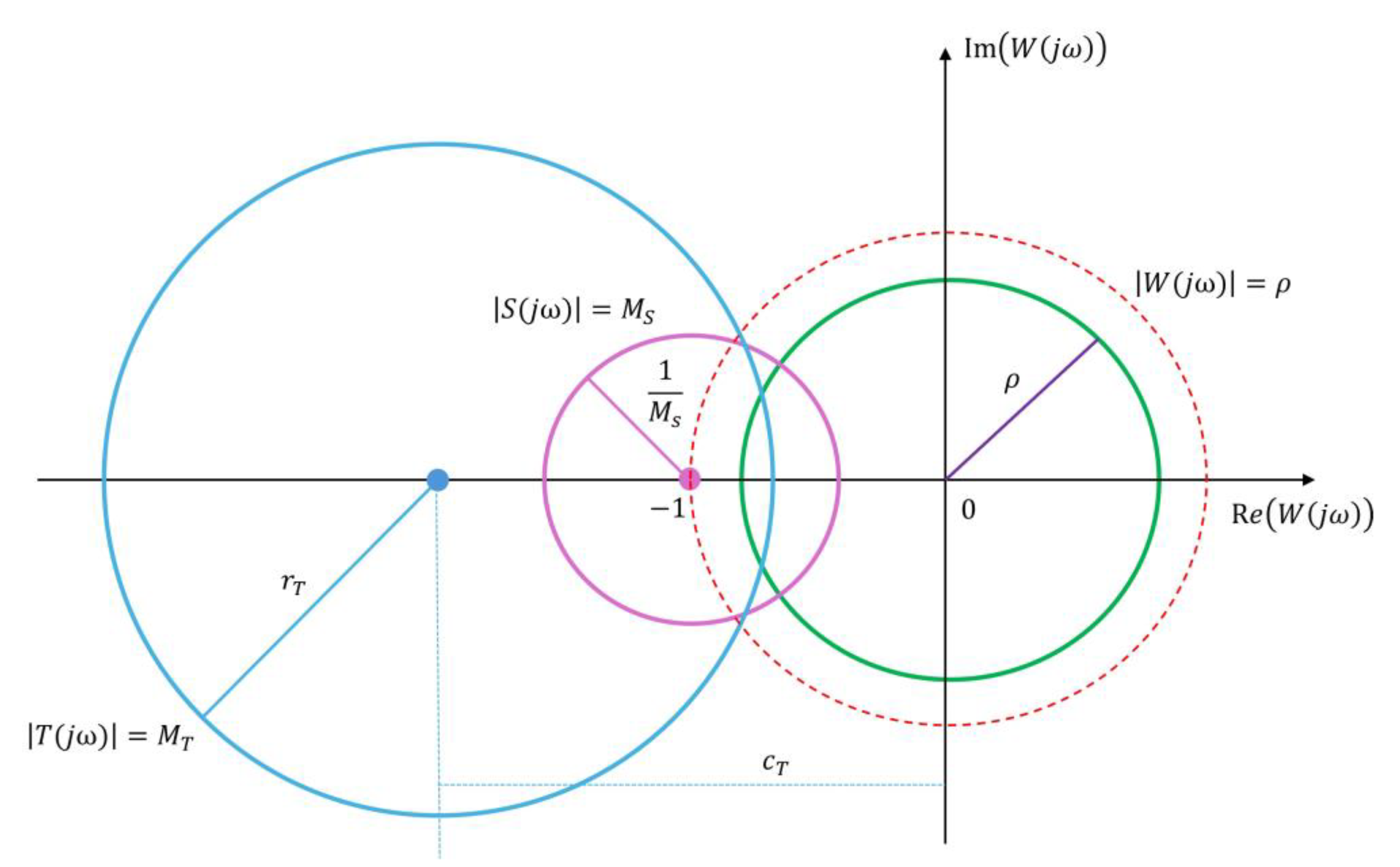
For the sensitivity function, using (7), condition (10) is obtained, which defines a circle with center at the point −1 and radius $1/M_S$ in the plane of $W$, Figure 1.

$$\left|S(j\omega )\right|=M_S⟺\left|1+W(j\omega )\right|={\displaystyle \frac{1}{M_S}}$$

(10)

Accordingly, the performance constraint (11) requires the frequency response of the open-loop system $W(j\omega )$to lie outside this circle.

$$\left|S(j\omega )\right|\le M_S$$

(11)

For the complementary sensitivity function, using (7), condition (12) is obtained.

$$\left|T(j\omega )\right|=M_T⟺\left|W\left(j\omega \right)\right|/\left|1+W(j\omega )\right|=M_T$$

(12)

For $M_T\ne 1$, condition (12) represents a circle in the plane of $W$with center $c_T$ and radius $r_T$ (13), Figure 1.

$$c_T=-{\displaystyle \frac{M_T^2}{M_T^2-1}},r_T={\displaystyle \frac{M_T}{\mid M_T^2-1\mid }}$$

(13)

where $c_T$ lies on the real axis to the left of −1.

Therefore, constraints on the modulus of $T(j\omega )$ also induce circular admissible sets in the Nyquist plane of the open-loop system.

In Figure 1, the different colors denote different types of frequency domain constraints. The green circle with center at the origin corresponds to the isomodular condition $\left|W\left(j\omega \right)\right|=\rho$, defined in (9).

The pink circle with center at point -1 and radius $1/M_S$ represents the sensitivity constraint formulated through (10), (11). The light blue circle corresponds to the complementary sensitivity constraint defined through (12), (13), while the dashed red circle denotes the unit circle.

In accordance with Geometric Statement 3.2, modulus level sets of fractional-linear functions of the complex variable $W$ define circles in the complex plane, or in the degenerate case, straight lines. Therefore, the constraints on $W$, $T$, and $S$ should not be regarded as geometrically different cases, but as realizations of the same geometric mechanism acting on the modulus of fractional-linear functions of $W$.

In accordance with Geometric Statement 3.3, circular constraints formulated in the frequency domain through modulus inequalities can be interpreted in the s-plane by considering the preimage of the admissible set.

This general geometric principle is used below to investigate the relationship between the isomodular circles shown in the Nyquist plane in Figure 1 and the locations of the dominant closed-loop poles.

4.1.1. General Case: Local Approximation around a Dominant Pole

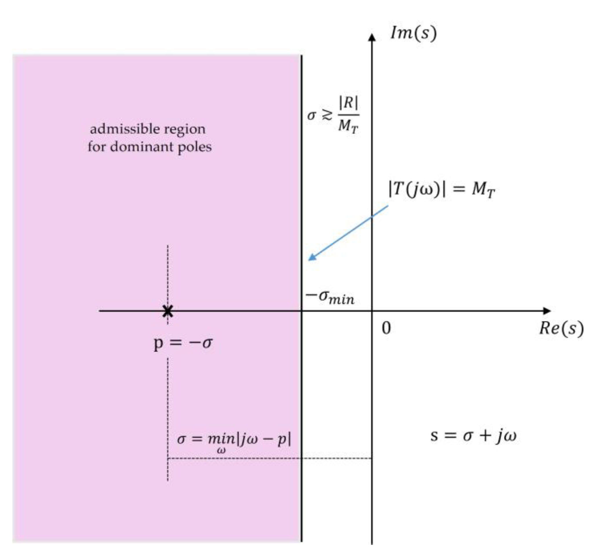
Let the closed-loop system $T(s)$ of (6) have a dominant pole $p=-\sigma$, located in the left half of the s-plane, Figure 2. About this pole, the complementary sensitivity can be approximated as (14), where $R$ is the residue of the complementary sensitivity $T(s)$ at the dominant pole $p$, defined as $R={\mathrm{l}\mathrm{i}\mathrm{m}}_{s\to p}(s-p)T(s)$.

This coefficient characterizes the local influence of the dominant pole on the dynamics of the closed-loop system.

$$T(s)\approx {\displaystyle \frac{R}{s-p}},$$

(14)

Along the frequency axis $s=j\omega$, the approximation (15) is obtained.

$$\left|T(j\omega )\right|\approx {\displaystyle \frac{\left|R\right|}{\left|j\omega -p\right|}}.$$

(15)

The minimum distance between the pole $p=-\sigma$and the frequency axis is equal to $\sigma$. Therefore, the maximum value of $T(j\omega )$can be estimated as (16).

$$\underset{\omega }{\mathrm{m}\mathrm{a}\mathrm{x}}\left|T(j\omega )\right|\approx {\displaystyle \frac{\left|R\right|}{\sigma }}.$$

(16)

If requirement (17) is imposed, from (16) the necessary condition (18) follows.

$$\left|T(j\omega )\right|\le M_T,\forall \omega ,$$

(17)

$$\sigma \gtrsim {\displaystyle \frac{\left|R\right|}{M_T}}.$$

(18)

Condition (18) has a geometric interpretation as a constraint on the radius of the isomodular circle associated with $\mid T\mid$(12) and leads to a minimum admissible horizontal distance of the dominant pole from the imaginary axis, denoted in Figure 2 by ${\sigma }_{\mathrm{m}\mathrm{i}\mathrm{n}}$.

This condition should be interpreted as a necessary local condition resulting from the dominant pole approximation.

In Figure 2, the admissible region for the location of the dominant closed-loop poles is indicated in light pink and corresponds to the geometric condition resulting from constraint (17) through the local approximation (14)–(16). The vertical dashed boundary $\mathrm{R}\mathrm{e}\left\{s\right\}=-{\sigma }_{\mathrm{m}\mathrm{i}\mathrm{n}}$ follows from the necessary condition (18), obtained from the maximum value of $\left|T(j\omega )\right|$, given in (16). In contrast to the constraint on $\left|T(j\omega )\right|$, which is directly related to the presence of oscillatory modes in control systems and allows a direct interpretation of transient behavior through the dominant closed-loop poles, the constraint on $\left|S(j\omega )\right|$, is used for a direct interpretation of robustness in the frequency domain.

Condition (10) defines the exterior of a circle with center at −1 in the Nyquist plane and can be interpreted as a minimum admissible distance of the open-loop frequency response from the critical point −1, providing a geometric measure of robustness.

It should be emphasized that a direct geometric relationship between the isomodular constraints (8) and the locations of the dominant poles is obtained in this form for the complementary sensitivity $T(s)$, due to the assumed real closed-loop pole locations. For the remaining modulus constraints (8), such a relationship requires additional assumptions, described in Section 4.1.2.

4.1.2. Special Case: System with Dominant Second-Order Dynamics

Let a closed-loop system be considered whose dominant dynamics can be described by a second-order model (19).

$$T(s)={\displaystyle \frac{{\omega }_n^2}{s^2+2\xi {\omega }_{n}s+{\omega }_n^2}}$$

(19)

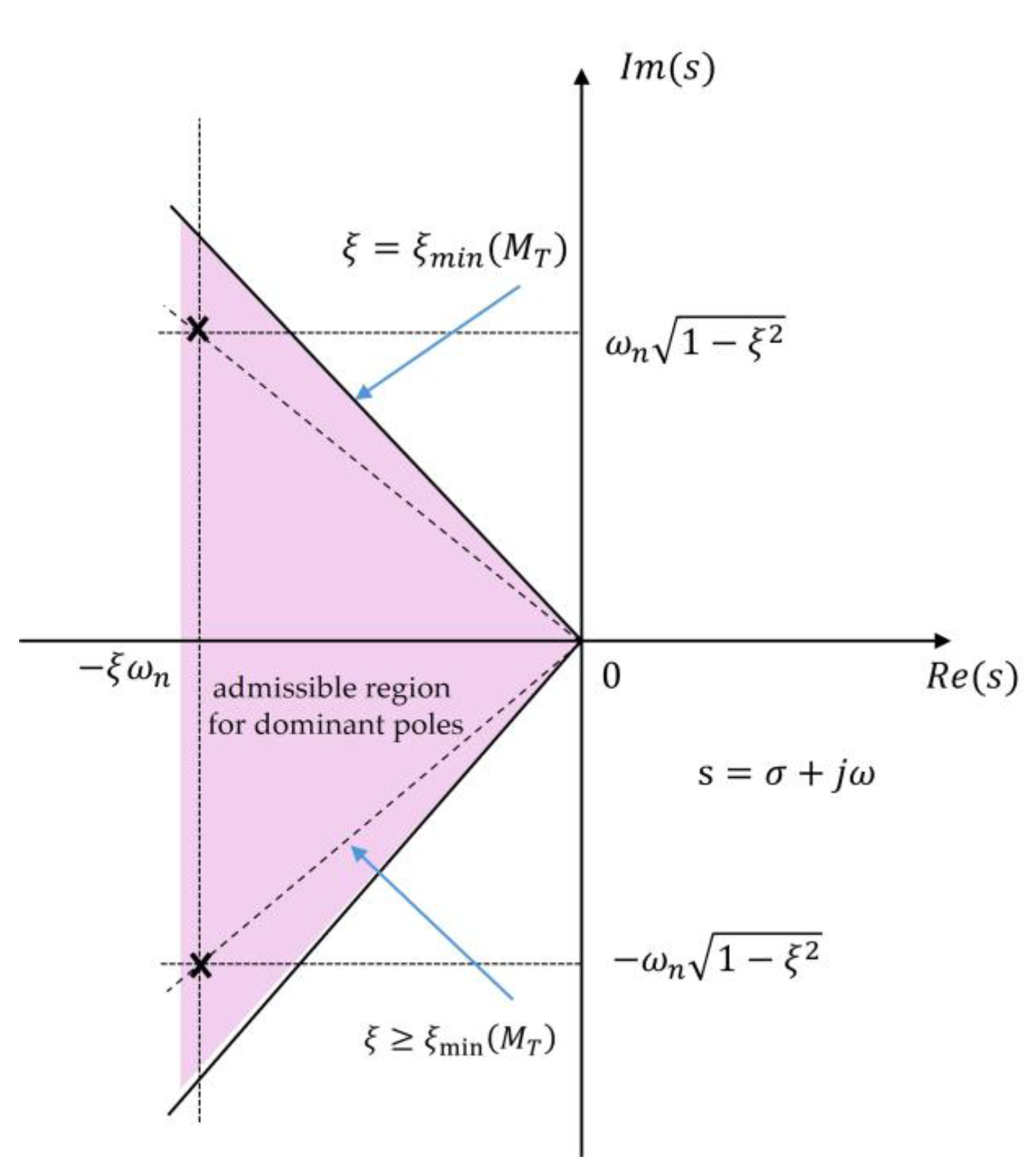
The dominant poles are located at $p_{\mathrm{1,2}}=-\xi {\omega }_n\pm j{\omega }_n\sqrt{1-{\xi }^2}$ in the s-plane, see Figure 3. It is well known that the maximum value of the modulus of the complementary sensitivity function is equal to the resonance peak, where the damping ratio $\xi$ appears explicitly in the relation (20).

$$M_T=\underset{\omega }{\mathrm{m}\mathrm{a}\mathrm{x}}\left|T(j\omega )\right|={\displaystyle \frac{1}{2\xi \sqrt{1-{\xi }^2}}},\xi <{\displaystyle \frac{1}{\sqrt{2}}}.$$

(20)

Expression (20) is valid for $\xi <1/\sqrt{2}$, when a resonance peak exists in the frequency response of the closed-loop system. For $\xi \ge 1/\sqrt{2}$, the maximum of $\left|T(j\omega )\right|$is attained at $\omega =0$ and is equal to unity. If constraint (17) is imposed on the complementary sensitivity function $T(s)$, inequality (21) follows, which leads to the formation of a lower bound for the damping ratio (22).

$${\displaystyle \frac{1}{2\xi \sqrt{1-{\xi }^2}}}\le M_T,$$

(21)

$$\xi \ge {\xi }_{\mathrm{m}\mathrm{i}\mathrm{n}}(M_T)=\sqrt{{\displaystyle \frac{1-\sqrt{1-1/M_T^2}}{2}}}.$$

(22)

It should be noted that condition (22) is meaningful for $M_T>1$, since for the closed-loop system $\left|T(j0)\right|=1$ and constraint of the form $\left|T(j\omega )\right|\le M_T<1$ cannot be satisfied. Thus, the constraint on the isomodulus circle associated with $\mid T(j\omega )\mid$, given in (17), defines an admissible region for the dominant poles specified by the minimum damping condition (22), see Figure 3.

In Figure 3, the admissible region for the placement of the dominant poles is indicated in light pink and corresponds to the geometric consequence of constraint (17) for a system with dominant second-order dynamics described by (19). The inclined boundaries of the region follow from the lower bound on the damping ratio given by (22), obtained from inequality (21) and the expression for the maximum of $\left|T(j\omega )\right|$ in (20).

The dominant poles $p_{\mathrm{1,2}}$ satisfy the condition $\xi \ge {\xi }_{\mathrm{m}\mathrm{i}\mathrm{n}}(M_T)$ and are located within this admissible region. The second-order case provides a structured realization of the general geometric mechanism discussed in Section 4.1.1. The isomodulus constraints on the frequency responses, formulated by (17) and represented as circular sets in the Nyquist plane of the complex function $W$ according to (12), lead to geometric quality constraints through the placement of the dominant closed-loop poles, as shown in (18) and (22). This relationship allows frequency domain performance requirements to be interpreted directly in the s-plane without introducing additional criteria, so that the isomodulus circles act as a universal geometric carrier of constraints in control theory.

4.2. Circles Induced by Robustness Margins

The classical stability margins in the frequency domain gain margin (GM) and phase margin (PM) impose constraints on the sensitivity $M_S$ (10) and complementary sensitivity $M_T$ (12) from the point of view of their geometric representation in the complex plane of the open-loop system $W(j\omega )$. The objective is to show that these seemingly different performance and stability measures can be described through a geometric mechanism based on circular admissible sets, in accordance with Geometric Statements 3.1–3.2.

The gain margin $GM$ is defined through an admissible scaling of the open-loop system by a factor $g$, such that the closed-loop system remains stable. In the Nyquist plane, this requirement can be formulated as a condition on the minimum distance between the frequency response of the open-loop system and the critical point −1. For requirement (23) imposed on $GM$, the equivalent condition on the modulus of the function $W(j\omega )$ is obtained in (24).

$$GM\ge g>1,$$

(23)

$$\left|1+W(j\omega )\right|\ge {\displaystyle \frac{g-1}{g}},\forall \omega ,$$

(24)

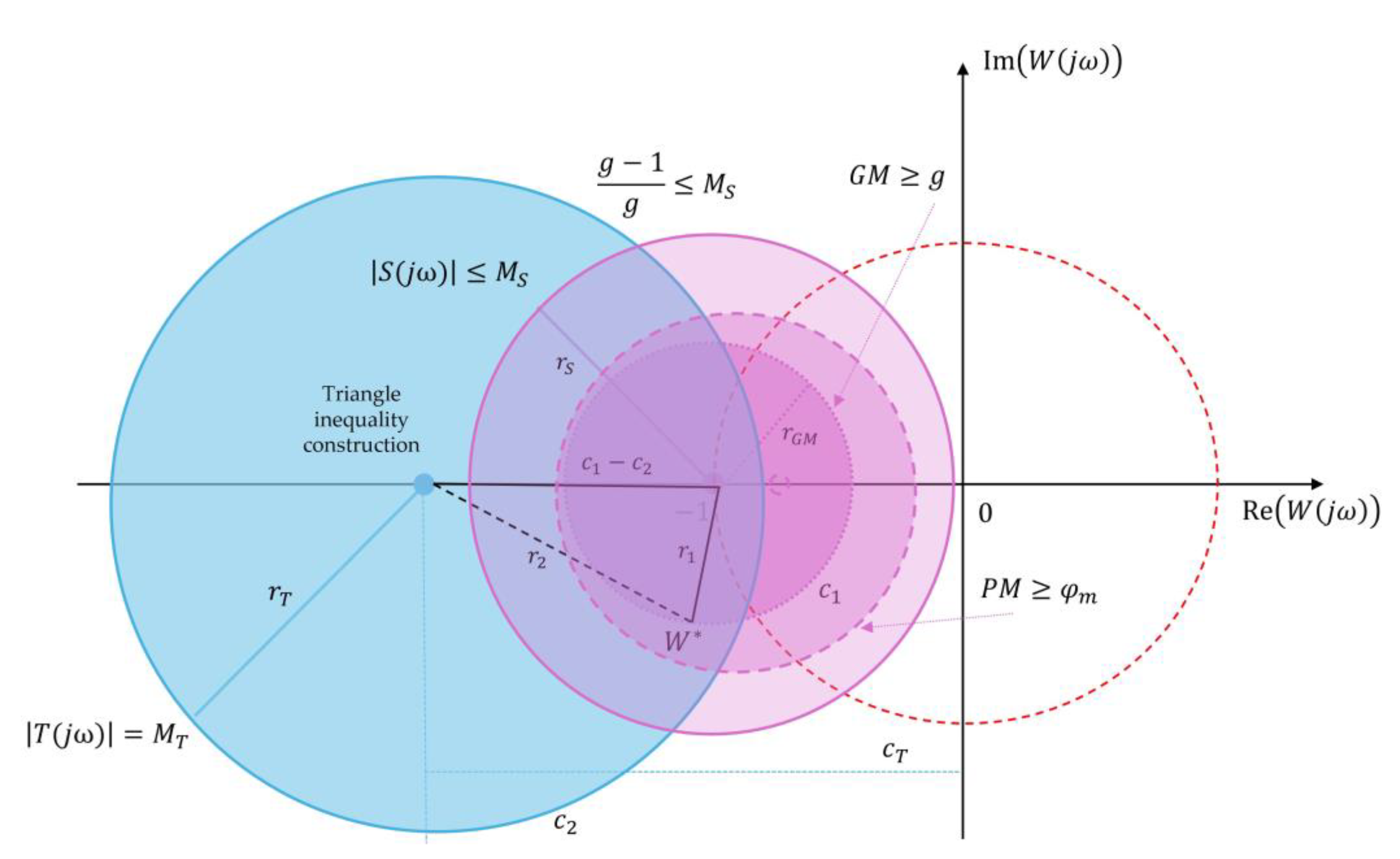
Condition (24) defines the exterior of a circle with center $c_{GM}$ and radius $r_{GM}$, see Figure 4 (25).

$$c_{GM}=-1,r_{GM}={\displaystyle \frac{g-1}{g}}$$

(25)

In a similar manner, the phase margin PM, although usually formulated as an angular condition at the intersection with the unit circle, also admits an equivalent representation through a constraint on the modulus of the complex function $W(j\omega )$. Let at the gain crossover frequency ${\omega }_{gc}$ condition (26) be satisfied.

$$\left|W(j{\omega }_{gc})\right|=1,\mathrm{a}\mathrm{r}\mathrm{g}W(j{\omega }_{gc})=-\pi +{\phi }_m.$$

(26)

Then (27) can be written.

$$W(j{\omega }_{gc})=e^{-j(\pi -{\phi }_m)}=-\mathrm{c}\mathrm{o}\mathrm{s}{\phi }_m+j\mathrm{s}\mathrm{i}\mathrm{n}{\phi }_m.$$

(27)

The distance from this point to the critical point −1 is given by (28).

$$\left|1+W(j{\omega }_{gc})\right|=\sqrt{\left(1-\mathrm{c}\mathrm{o}\mathrm{s}{\phi }_m{)}^2+{\mathrm{s}\mathrm{i}\mathrm{n}}^2{\phi }_m=2\mathrm{s}\mathrm{i}\mathrm{n}{\displaystyle \frac{{\phi }_m}{2}}\right.}$$

(28)

Therefore, the condition for a minimum phase margin takes the form (29) and is equivalent to a modulus constraint on $W(j\omega )$ (30), which defines the exterior of a circle with center −1 and radius $r_{PM}$, see Figure 4.

$$PM\ge {\phi }_m$$

(29)

$$\left|1+W(j\omega )\right|\ge r_{PM},r_{PM}=2\mathrm{s}\mathrm{i}\mathrm{n}{\displaystyle \frac{{\phi }_m}{2}}$$

(30)

The obtained circular constraint (30) is equivalent to the classical definition of the phase margin $PM$ at the gain crossover frequency ${\omega }_{gc}$. In this way, the phase margin $PM$ is reduced to a circular constraint in the Nyquist plane and represents a special case of a constraint in accordance with Geometric Statement 3.1.

As shown in section 4.1, the constraints on sensitivity and complementary sensitivity (10) and (12) define circular admissible sets in the complex plane of the function $W(j\omega )$.

In particular, the sensitivity constraint is equivalent to (11), which defines the exterior of a circle with center $c_S=-1$ and radius $r_S=1/M_S$. The complementary sensitivity constraint (12) leads to a circle with center and radius given by (13).

It is important to emphasize that, despite their different engineering interpretations, the gain margin $GM$, the phase margin $PM$, and the indices $M_S$ and $M_T$ lead to constraints of the same geometric type, namely a requirement that the frequency response of the open-loop system belongs to the exterior or interior of a given circle in the complex plane. Let two constraints be represented by circles (31).

$$C_1=\{W:\left|W-c_1\right|\le r_1\}, C_2=\{W:\left|W-c_2\right|\le r_2\}.$$

(31)

The inclusion condition is given by the union of the circles (32), (33) and has a simple geometric form given by (34), which follows directly from the triangle inequality, see Figure 4.

$$\left|W-c_2\right|\le \left|W-c_1\right|+\left|c_1-c_2\right|=r_1+\left|c_1-c_2\right|$$

(32)

$$C_1\subseteq C_2$$

(33)

The condition $C_1\subseteq C_2$ means that the admissible set defined by constraint $C_1$ is included in the admissible set $C_2$, so that satisfying the first constraint guarantees satisfaction of the second one.

$$\left|c_1-c_2\right|\mathrm{ }+r_1\le r_2,$$

(34)

Condition (34) follows from the triangle inequality (32), see Figure 4. For the typical case in which the phase of the open-loop frequency response reaches the value −π at a single frequency ${\omega }_{-\pi }$, the complex value of $W(j\omega )$ at this point is real and negative and can be written in the form (35).

$$W(j{\omega }_{-\pi })=-a,0<a<1.$$

(35)

From the sensitivity constraint (11), condition (36) follows, which leads to the inequality $a\le 1-{\displaystyle \frac{1}{M_S}}.$

$$\left|1+W(j{\omega }_{-\pi })\right|=\left|1-a\right|\ge {\displaystyle \frac{1}{M_S}},$$

(36)

Since the gain margin $GM$ is defined as (37), from (36) the lower bound (38) is obtained.

$$GM={\displaystyle \frac{1}{a}},$$

(37)

$$GM\ge {\displaystyle \frac{M_S}{M_S-1}}.$$

(38)

Equivalently, for a given requirement on the gain margin $GM\ge g$, it is sufficient that condition (39) be satisfied.

$$M_S\le {\displaystyle \frac{g}{g-1}}.$$

(39)

In geometric terms, this means that the radius of the circle $r_S$, associated with the sensitivity constraint (11), is not smaller than the radius of the circle $r_{GM}$, associated with the gain margin (24).

$$r_S\ge {\displaystyle \frac{g-1}{g}}=r_{GM}.$$

(40)

Geometrically, condition (40) means that the circle associated with the gain margin (a circle centered at −1 with a smaller radius, shown with a fine dashed line) is entirely included in the circle associated with the sensitivity constraint (a circle centered at −1 with a larger radius, shown with a solid line), as illustrated in Figure 4.

The robustness and performance requirements defined through the sensitivity constraint (11), the gain margin (23), and the phase margin (29) lead to constraints on the modulus of the complex function$\left|1+W(j\omega )\right|$. In particular, the corresponding conditions can be written in the form (41).

$$\left|1+W(j\omega )\right|\ge r_{GM},\left|1+W(j\omega )\right|\ge r_{PM},\left|1+W(j\omega )\right|\ge r_S,$$

(41)

where the radii $r_{GM}$, $r_{PM}$, and $r_S$ are defined in (25), (30), and (10), (11), respectively.

Therefore, these requirements can be unified into a single combined geometric condition of the form (42).

$$\left|1+W(j\omega )\right|\ge r^{*}\mathrm{ },\forall \omega ,$$

(42)

where the effective radius $r^{*}$ is defined as (43).

$$r^{*}\mathrm{ }=\mathrm{m}\mathrm{a}\mathrm{x}\{r_{GM},r_{PM},r_S\}.$$

(43)

In addition, the complementary sensitivity constraint (17) defines an additional admissible set in the Nyquist plane, given by a circle with center $c_T$ and radius $r_T$, (44), where the parameters $c_T$ and $r_T$ are defined in (13).

$$\left|W(j\omega )-c_T\right|\le r_T.$$

(44)

Figure 4 illustrates the overlapping circular constraints induced by the different requirements on gain margin $GM$, phase margin $PM$, the sensitivity $S$, and the complementary sensitivity $T$ in the plane of the frequency response of the open-loop system. The inclusion of one circle within another visualizes the geometric conservatism of the constraints and shows that different robustness requirements may lead to the same admissible region.

The shaded region (the densest area) in Figure 4 represents the intersection of the circular admissible sets associated with the individual constraints (11), (23), and (29) and defines a common geometric region in the Nyquist plane in which the placement of the frequency response of the open-loop system $W\left(j\omega \right)$constitutes a sufficient condition for the simultaneous satisfaction of the gain margin, phase margin, sensitivity, and complementary sensitivity requirements. Formally, this admissible region can be described by the set (45).

$$\mathcal{A}=\{W\in \mathbb{C}:\left|1+W\right|\ge r_{*}\}\cap \{W\in \mathbb{C}:\left|W-c_T\right|\le r_T\},$$

(45)

where the effective radius $r_{*}$ is defined in (43), with radii $r_{GM}$, $r_{PM}$, and $r_S$ given in (25), (30), and (12), respectively, and the parameters $c_T$ and $r_T$ defined in (13).

The first condition in $\mathcal{A}$ excludes a circle centered at the critical point −1, while the second condition constrains the frequency response within the circle associated with the complementary sensitivity, as derived in §4.1.

The classical performance measures gain margin, phase margin, as well as the indices $M_S$ and $M_T$ can be regarded as special cases of the same class of circular geometric constraints. This makes it possible to compare and combine them at a geometric level through circle inclusion conditions and minimum radii that guarantee the simultaneous satisfaction of different robustness requirements.

4.3. Frequency-Dependent Families of Circles

In accordance with Geometric Statements 3.1–3.2, the requirements in the frequency domain formulated through modulus inequalities induce not single circular constraints, but families of circles in the Nyquist plane, parameterized by the frequency $\omega$. An illustration of a frequency-dependent family of circles is given in Figure 5, where the circular boundary varies while preserving the underlying geometric interpretation.

Let a frequency domain constraint be defined in the Nyquist plane of $W(j\omega ),$ which for each frequency $\omega$ induces a circle (46).

$$C\left(\omega \right)=\left\{W\in \mathbb{C}: \left|W-c\left(\omega \right)\right|=r\left(\omega \right)\right\},\omega \in \left[0,\mathrm{\infty }\right).$$

(46)

The set $C(\omega )$ describes the geometric boundary of the constraint, while the admissible region $D(\omega )$ is defined as the interior or the exterior of this circle, depending on the sign of the corresponding inequality (11).

The corresponding admissible set $D$ is defined as the intersection of the admissible regions $D(\omega )$ over all frequencies (when the requirement must hold for all $\omega$), (47).

$$D=\bigcap _{\omega \ge 0}D(\omega ),$$

(47)

The intersection (47) expresses the requirement that the frequency domain constraint must be satisfied for all frequencies $\omega$, which leads to an admissible set $D$ determined by the most restrictive circle in the family.

If requirement (11) is imposed, then, using relation (7), the equivalent condition (48) is obtained.

$$\left|1+W(j\omega )\right|\ge {\displaystyle \frac{1}{M_S(\omega )}}.$$

(48)

Therefore, for each frequency $\omega$, a circle is obtained in the $W$- Nyquist plane (49).

$$\left|W-(-1)\right|={\displaystyle \frac{1}{M_S(\omega )}}.$$

(49)

In this case, its center $c_S(\omega )$ is fixed (50) and the radius $r_S(\omega )$ depends on the frequency $\omega$ (51).

$$c_S(\omega )\equiv -1,$$

(50)

$$r_S(\omega )={\displaystyle \frac{1}{M_S(\omega )}}$$

(51)

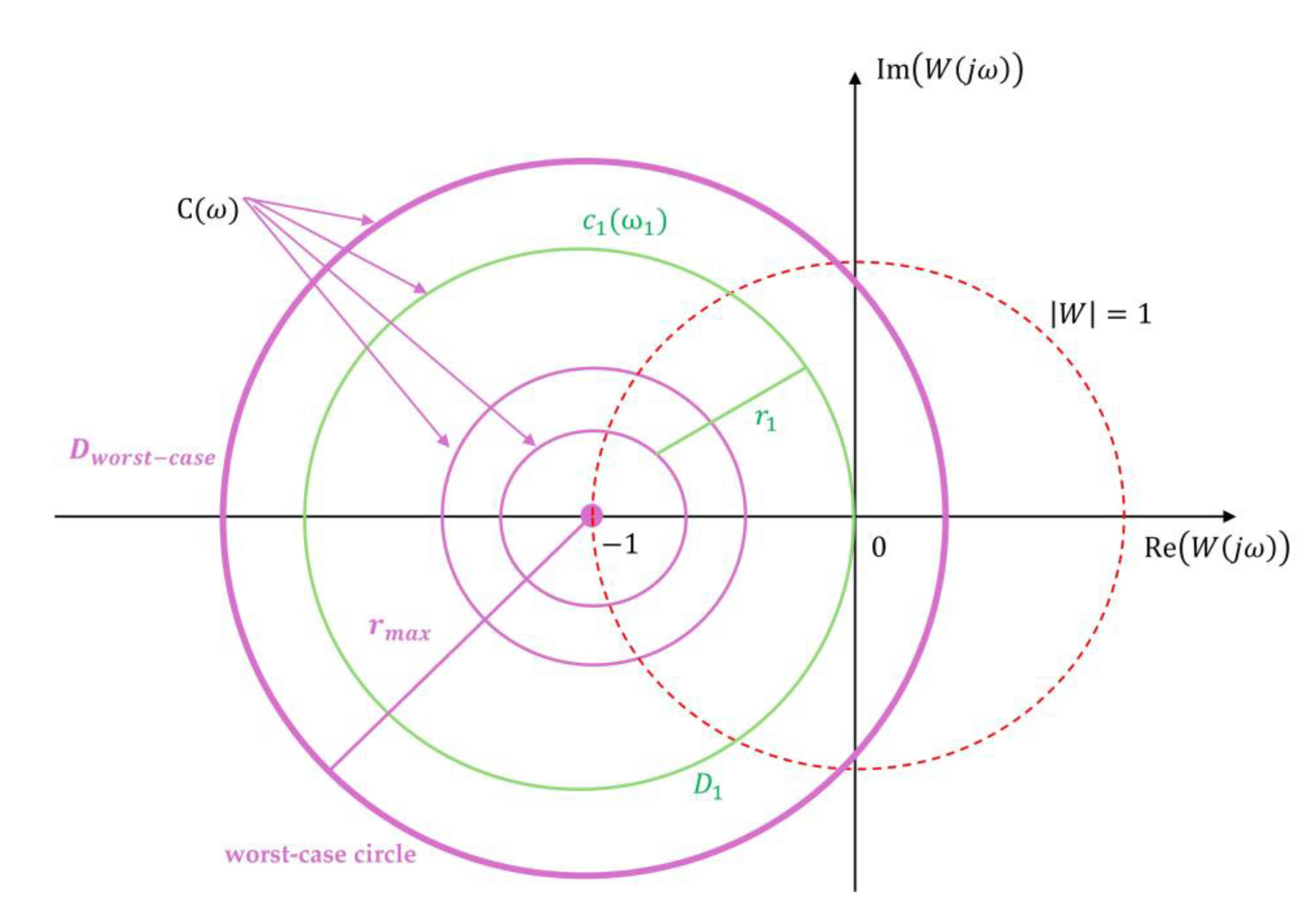
The admissible set $D(\omega )$ represents the exterior of each circle in the family $C(\omega )$, i.e., the frequency response of the open-loop system must lie outside all circles around the critical point $-1$, as shown in Figure 5.

When the family of circles has a fixed center $c(\omega )\equiv c$ (as in the constraints on $S$, $GM$, and $PM$), the frequency domain constraint can be reduced to a single dominant (most conservative) circle. If the constraint is of the “exterior” type (52), then it is sufficient (and in this case equivalent) that (53) holds, where the critical frequency ${\omega }^{\star }$ is defined by (54).

$$\left|W-c\right|\ge r(\omega ),\forall \omega ,$$

(52)

$$\left|W-c\right|\ge r_{\mathrm{m}\mathrm{a}\mathrm{x}},r_{\mathrm{m}\mathrm{a}\mathrm{x}}=\underset{\omega \ge 0}{\mathrm{m}\mathrm{a}\mathrm{x}}r(\omega ),$$

(53)

$${\omega }^{\star }\in \mathrm{a}\mathrm{r}\mathrm{g}\underset{\omega \ge 0}{\mathrm{m}\mathrm{a}\mathrm{x}}r(\omega ).$$

(54)

When $c(\omega )$ and/or $r(\omega )$ vary with the frequency $\omega$ (for example, when $M_S\left(\omega \right)$and $M_T(\omega )$ are considered simultaneously), the geometric constraint can no longer be adequately described by a single circle. In this case, the boundary object is the envelope of the family $C(\omega )$, which defines the actual boundary of the admissible set.

Let $W=x+jy$. The circle $C(\omega )$ is defined by (55).

$$f(W,\omega )={\left|W-c(\omega )\right|}^2 -r(\omega {)}^2=0.$$

(55)

The envelope of the family is obtained from the system (56). This construction assumes that the functions $c(\omega )$ and $r(\omega )$ are sufficiently smooth so that the envelope is well defined.

$$\left\{\begin{array}{c}f(W,\omega )=0,\\ {\displaystyle \frac{\partial f}{\partial \omega }}(W,\omega )=0.\end{array}\right.$$

(56)

Equations (56) determine those frequencies $\omega$ at which the current circle is tangent to the boundary curve of the family and thus becomes active, i.e., locally determines the geometry of the admissible region.

The geometric interpretation of conditions (46)–(56) is shown in Figure 5. The family of frequency-dependent circles $C(\omega )$, defined by (46), is illustrated in light pink, where each circle corresponds to a fixed frequency $\omega$. The green circle denotes the dominant (worst-case) circle, determined by the maximum value of the radius $r(\omega )$ according to (53), attained at the critical frequency ${\omega }^{\star }$, defined in (54). The dashed red curve represents the geometric envelope of the family $C(\omega )$, obtained from the tangency conditions (55), (56), which defines the actual boundary of the admissible set in cases where reduction to a single dominant circle is not possible.

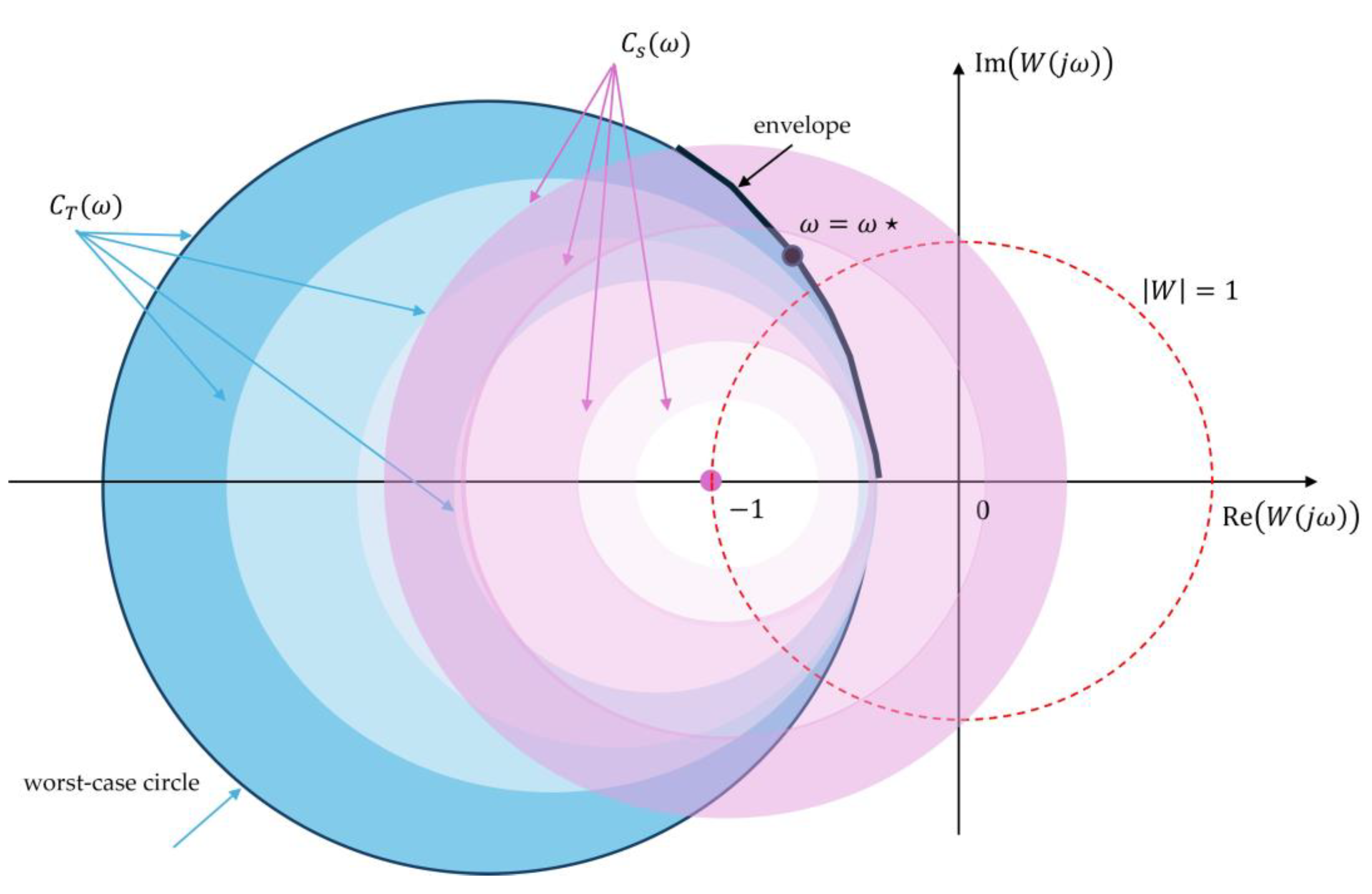
In the case of combined frequency-dependent constraints, for example the simultaneous action of sensitivity constraints given by the circle $C_S(\omega )$ (of “exterior” type) and complementary sensitivity constraints $C_T(\omega )$ (of “interior” type), the admissible set is defined as the intersection of the exteriors and interiors of the corresponding circles, defined respectively by (46) and the associated frequency-dependent modulus inequalities (11) and (12).

In Figure 6, a case is considered in which the frequency-dependent constraints on complementary sensitivity are of the “interior” type ($M_T(\omega )<1$), so that $C_T(\omega )$ describe interior circles in the Nyquist plane, while the more general case $M_T(\omega )\ge 1$ and its related geometric generalizations are discussed in Section 5. In this situation, the active boundary is not determined by a single circle, but by an envelope that may consist of arcs from both exterior and interior circular constraints, active at different frequencies as defined by system (56).

The light blue regions correspond to the frequency-dependent exterior circular constraints induced by conditions of type (11) through the circles $C_S(\omega )$, defined by (46). The light pink regions correspond to the interior circular constraints induced by conditions of type (12) for the complementary sensitivity $T$. The black curve represents the active geometric envelope of the combined family of circular constraints, obtained from the tangency conditions (55)–(56). The marked point on the envelope corresponds to the critical frequency ${\omega }^{\star }$, at which the corresponding frequency-dependent constraint becomes active and locally determines the geometry of the admissible set.

Therefore, synthesis can be interpreted as a geometric shaping of the Nyquist locus such that it remains within the admissible region and does not intersect the envelope, while the critical frequency ${\omega }^{\star }$ indicates the frequency at which the robustness constraints become determining.

The frequency-domain constraints are thus interpreted geometrically as families of circular sets in the Nyquist plane, parameterized by the frequency $\omega$. The admissible region is determined by the active elements of this family, which realize the most restrictive condition.

In accordance with Geometric Statement 3.3, these circular sets in the frequency domain are subsequently considered through their preimage in the complex $s$-plane, which allows a direct interpretation in terms of the location of the dominant poles.

4.4. Preimages of Frequency-Domain Circles in the s-Plane

The circular admissible sets in the frequency domain, in the Nyquist plane of the complex function $W(j\omega )$, arise as isomodular level sets of analytic or fractional-linear functions of $W$ and are directly related to robust stability and robust performance conditions.

In this subsection, the geometric mechanism is examined through which these frequency-formulated circular constraints are transferred to the $s$-plane, in accordance with Geometric Statement 3. The main objective is to show how frequency domain robustness conditions lead to admissible regions for the location of the dominant poles of the closed-loop system.

4.4.1. Preimage of a Frequency-Domain Circular Constraint

Let the frequency-domain constraint be defined by a circular set in the complex plane of $W$ (3). The preimage of this set in the complex $s$-plane is defined as in (5). The resulting set $S$ represents an admissible region for the location of the closed-loop poles, obtained from the frequency domain constraint. In this way, frequency requirements are not interpreted in isolation but are translated into geometric constraints on the system dynamics.

Robust stability and robust performance requirements in control theory are most often formulated in the frequency domain through conditions of the form (57) and (58), which define robust stability $RS$and robust performance $RP$, respectively.

$$\underset{\omega \ge 0}{\mathrm{s}\mathrm{u}\mathrm{p}}\left|l_m\left(j\omega \right)T\left(j\omega \right)\right|\le 1\mathrm{ }$$

(57)

$$\underset{\omega \ge 0}{\mathrm{s}\mathrm{u}\mathrm{p}}\left|l_m(j\omega )T(j\omega )+y^0(j\omega )S(j\omega )\right|\le 1$$

(58)

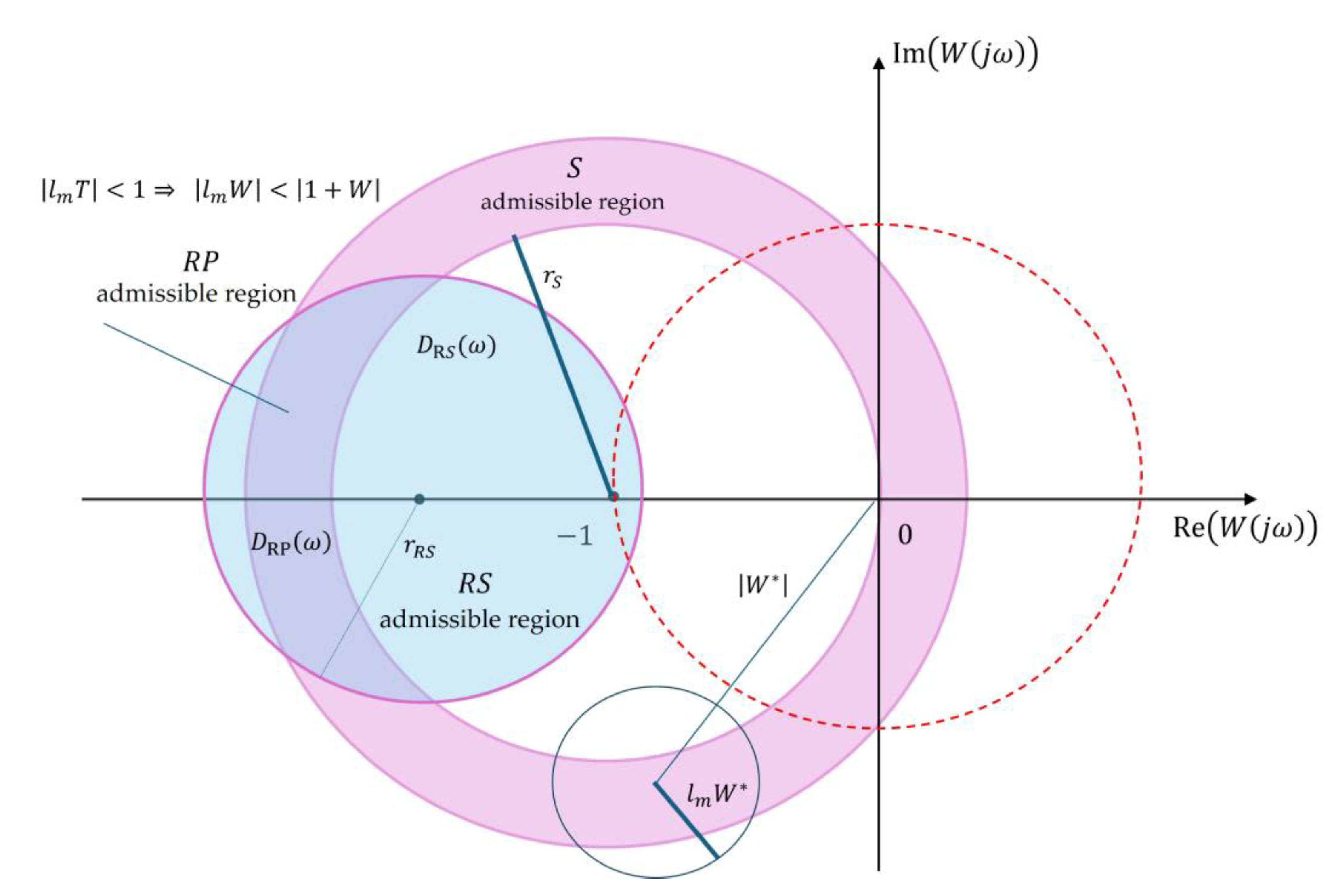
The function $l_m(j\omega )$ is interpreted as a multiplicative perturbation describing the admissible relative deviation of the real system from its nominal model. Due to the modulus form of constraints (57), (58), this multiplicative effect leads to circular admissible sets, where $\left|l_m(j\omega )\right|$ determines the effective radius of the corresponding constraint without altering its geometric form, Figure 7. The additive term $y^0(j\omega )S(j\omega )$ models an additive effect that shifts the center of the corresponding circular constraint without changing its circular character, Figure 7.

These inequalities have the form of modulus constraints on complex functions of $W(j\omega )$, in accordance with (2), (3) and represent circular admissible sets in the Nyquist plane. The quantity $\left|W^{\mathrm{*}}\right|$ denotes the magnitude of the frequency response of the nominal open-loop control system at the frequency at which the corresponding robustness constraint becomes active (worst-case), while the radii of the circular admissible sets are determined by the magnitudes of the frequency-dependent multipliers in conditions (57), (58), Figure 7.

Geometrically, $RP$ corresponds to a smaller radius and leads to a nested admissible region with respect to $RS.$ It should be noted that in the case of robust performance, the circular constraint is combined with an additional condition arising from the additive term $y^0(j\omega )S(j\omega )$. Geometrically, this results not in a full circle but in an admissible sector of the corresponding circular set, as shown in Figure 7.

For each fixed frequency $\omega$, conditions (57) and (58) define admissible sets in the Nyquist plane which, according to Geometric Statements 3.1–3.2, have a circular character. Let these sets be denoted by $D_{RS}(\omega )$ and $D_{RP}(\omega )$, respectively. Due to the presence of the additional term containing the sensitivity $S(j\omega )$, the robust performance condition is more restrictive, which is geometrically expressed by the inclusion (59).

$$D_{\mathrm{R}\mathrm{P}}\left(\omega \right)\subseteq D_{\mathrm{R}\mathrm{S}}\left(\omega \right),\forall \omega \ge 0.$$

(59)

After intersection over all frequencies, the inclusion of the global admissible sets is obtained (60).

$$D_{\mathrm{R}\mathrm{P}}=\bigcap _{\omega \ge 0}{D}_{\mathrm{R}\mathrm{P}}(\omega )\subseteq \bigcap _{\omega \ge 0}{D}_{\mathrm{R}\mathrm{S}}(\omega )=D_{\mathrm{R}\mathrm{S}}$$

(60)

Here $D_{RS}(\omega )$ denotes the local admissible set at frequency $\omega$, whereas $D_{RS}$ denotes the global set obtained after intersection over $\omega \ge 0$In Figure 7, this inclusion is visualized by the embedding of the light-blue region, corresponding to the$RS$ admissible set $D_{RS}(\omega )$, within the light-pink region corresponding to the S admissible set, while the darker left region denotes the $RP$ admissible set $D_{RP}(\omega )$.

4.4.2. Local Interpretation of the Preimage in the s-Plane

According to Geometric Statement 3, the preimage of a defined set in the frequency domain preserves this inclusion, i.e., (61).

$$S_{\mathrm{R}\mathrm{P}}=W^{-1}(D_{\mathrm{R}\mathrm{P}})\subseteq W^{-1}(D_{\mathrm{R}\mathrm{S}})=S_{\mathrm{R}\mathrm{S}}.$$

(61)

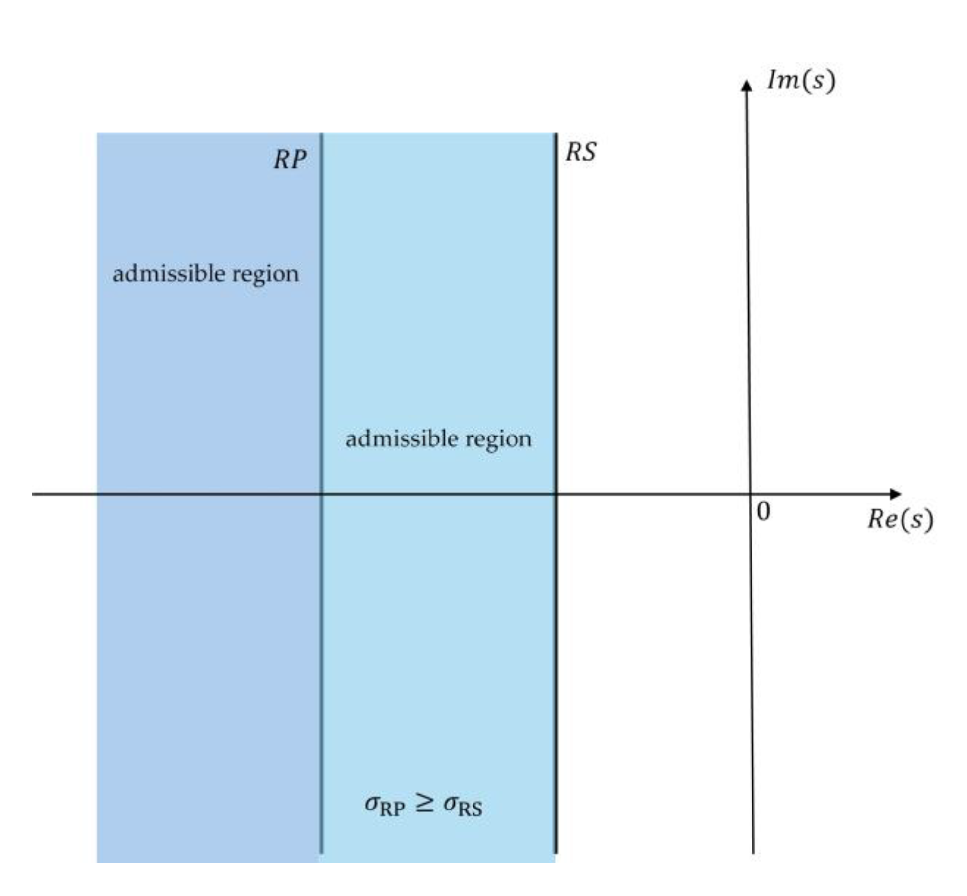
Therefore, robust performance imposes a stricter admissible region in the s-plane, embedded within the region guaranteeing robust stability, i.e., (62).

$${\sigma }_{\mathrm{R}\mathrm{P}}\ge {\sigma }_{\mathrm{R}\mathrm{S}},{\xi }_{\mathrm{R}\mathrm{P}}\ge {\xi }_{\mathrm{R}\mathrm{S}}.$$

(62)

According to Geometric Statement 3, every circular constraint in the frequency domain, defined by (2), (3), generates an admissible region in the s-plane through its preimage $S$, given by (5). In this way, the frequency domain conditions for robust stability and robust performance ($RS$ and $RP$), defined by (57), (58), are interpreted as geometric constraints on the closed-loop poles locations.

In the presence of dominant closed-loop poles, the preimage of the circular frequency domain constraints can be analyzed locally in the s-plane.

(a) Dominant simple pole

Let $p$ be a dominant simple pole of the closed-loop control system. In its neighborhood, the complementary sensitivity $T(s)$ can be approximated as (63).

$$T(s)\approx {\displaystyle \frac{\left|R\right|}{s-p}}$$

(63)

where $R$ denotes the residue of $T(s)$ at the dominant pole.

Along the frequency axis $s=j\omega$, from (63) it follows that (64).

$$\left|T(j\omega )\right|\approx {\displaystyle \frac{\left|R\right|}{\mid j\omega -p\mid }}.$$

(64)

The imposed frequency domain constraint on the complementary sensitivity $T(s)$ (17) leads to the condition (65).

$$\left|j\omega -p\right|\ge {\displaystyle \frac{\left|R\right|}{M_T}},\forall \omega .$$

(65)

From inequality (65), a minimum admissible horizontal distance of the dominant pole from the imaginary axis follows, expressed by (66).

$$\mathrm{R}\mathrm{e}\left\{p\right\}\le -{\sigma }_{\mathrm{m}\mathrm{i}\mathrm{n}},{\sigma }_{\mathrm{m}\mathrm{i}\mathrm{n}}={\displaystyle \frac{\left|R\right|}{M_T}}.$$

(66)

In this way, the frequency domain constraint on the modulus of the complementary sensitivity (66) is interpreted as a vertical boundary in the s-plane, limiting the admissible location of the dominant pole, Figure 8a.

(b) Dominant second-order dynamics

For a system with dominant second-order dynamics, the constraint on the complementary sensitivity $T(s)$, defined by (15), leads to a lower bound on the damping ratio $\xi$, which can be written in the form (67).

$$\xi \ge {\xi }_{\mathrm{m}\mathrm{i}\mathrm{n}}(M_T),$$

(67)

Geometrically, condition (67) defines a wedge-shaped admissible region in the s-plane, bounded by straight lines forming a constant angle with the real axis, where the angle is related to the damping ratio through the relation $\xi =\mathrm{c}\mathrm{o}\mathrm{s}\phi$.

The obtained geometric interpretation is illustrated in Figure 8b, where the preimage of the frequency domain constraint on $T$ is shown as a wedge-shaped admissible region in the s-plane.

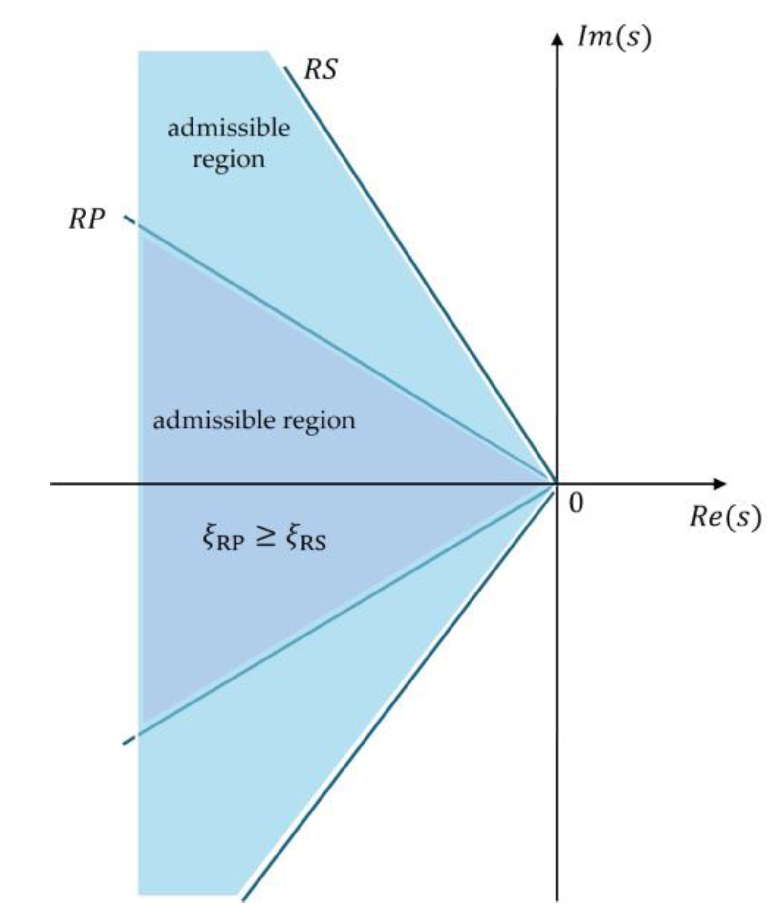
Figure 8 illustrates the inclusion $S_{RP}\subseteq S_{RS}$ both for a dominant simple pole (Figure 8a) and for second-order dynamics (Figure 8b), where $RS$ is indicated in light blue and $RP$ in darker blue.

4.4.3. Admissible Regions for RS and RP and Combined Constraints

The frequency domain constraints RS and RP, (57) and (58), represented as circular sets in the Nyquist plane (Figure 8a), define through their preimages two admissible regions in the s-plane (Figure 8b) the region $S_{RS}$, guaranteeing robust stability, and the region $S_{RP}\subseteq S_{RS}$, guaranteeing robust performance.

For a dominant simple pole, the robust stability constraint leads to condition (68), while the combined frequency domain constraint for robust performance imposes a stricter boundary (69).

$$\mathrm{Re}\left\{p\right\}\le -{\sigma }_{\mathrm{R}\mathrm{S}},{\sigma }_{\mathrm{R}\mathrm{S}}={\displaystyle \frac{R}{M_T}},$$

(68)

$$\mathrm{Re}\left\{p\right\}\le -{\sigma }_{\mathrm{R}\mathrm{P}},{\sigma }_{\mathrm{R}\mathrm{P}}\ge {\sigma }_{\mathrm{R}\mathrm{S}}.$$

(69)

Therefore, the simultaneous satisfaction of the robust stability and robust performance conditions requires (70).

$$\mathrm{R}\mathrm{e}\left\{p_{\mathrm{d}\mathrm{o}\mathrm{m}}\right\}\le -\mathrm{m}\mathrm{a}\mathrm{x}\{{\sigma }_{\mathrm{R}\mathrm{S}},{\sigma }_{\mathrm{R}\mathrm{P}}\}.$$

(70)

For a control system with dominant second-order dynamics, an analogous combined angular constraint (71) is obtained, which defines a single admissible region guaranteeing simultaneous robust stability and robust performance.

$$\xi \ge \mathrm{m}\mathrm{a}\mathrm{x}({\xi }_{RS},{\xi }_{RP}),$$

(71)

Equations (70) and (71) allow the frequency domain requirements for stability and performance to be used directly in the synthesis, without the need for repeated frequency checks. The design of the control algorithm can be interpreted as the selection of parameters that place the dominant poles inside the admissible region $S_{RS}$ or $S_{RP}$, defined through the preimage (5) of the frequency domain constraints (57), (58). In this way, frequency domain robust analysis and s-plane analysis can be unified into a single geometric design tool. Thus, the frequency domain constraints $RS$ and $RP$ obtain a direct interpretation as geometric conditions on the location of the dominant poles.

4.5. Circular Constraints and Performance Indices

The circular constraints in the frequency domain used for robust stability $RS$ and robust performance $RP$, defined by (57) and (58), impose direct numerical constraints on the most commonly used time domain performance indicators of the closed-loop control system, namely the settling time $t_s$ and the percent overshoot ${\sigma ,}_{\mathrm{\%}}$. Unlike the classical time domain analysis, where speed of response and overshoot are evaluated through transient responses, here these indicators are interpreted geometrically through the admissible regions in the s-plane obtained from the preimages (5) of the circular constraints defined in the frequency domain.

Let the closed-loop system $T(s)$ have dominant second-order dynamics described by the complex conjugate pair of poles (19). The classical time domain performance measures of the closed-loop control system can be approximated by the following relations, valid for dominant second-order dynamics (72).

$$t_s\approx {\displaystyle \frac{4}{\xi {\omega }_n}},{ \sigma }_{\%}={е}^{-{\displaystyle \frac{\pi \xi }{\sqrt{1-{\xi }^2}}}},$$

(72)

The frequency domain constraint for robust stability introduced in (17) and used locally in (65), through the local approximation around the dominant closed-loop pole (50), leads to the estimate along the frequency axis (64). From inequality (65), a minimum horizontal distance of the dominant poles from the imaginary axis follows, expressed by (66). The geometric constraint (66) directly provides numerical bounds on the time domain performance indicators. In particular, using the relation for the settling time given in (72), an upper bound on the settling time is obtained (73).

$$t_s\le {\displaystyle \frac{4}{{\sigma }_{\mathrm{m}\mathrm{i}\mathrm{n}}}}={\displaystyle \frac{4M_T}{\mid R\mid }}.$$

(73)

From (73), a lower bound on the undamped natural frequency ${\omega }_n$ follows (74).

$${\omega }_n\ge {\displaystyle \frac{{\sigma }_{\mathrm{m}\mathrm{i}\mathrm{n}}}{\xi }}={\displaystyle \frac{\left|R\right|}{M_T\xi }}.$$

(74)

In addition to the constraint on the real part (66), for dominant second-order dynamics the frequency domain constraint on the complementary sensitivity (17) also leads to a lower bound on the damping ratio $\xi$, as obtained in (22). Since the percent overshoot ${\sigma ,}_{\mathrm{\%}}$ is a monotonically decreasing function of $\xi$ for $\xi \in (\mathrm{0,1})$, it follows from (72) that constraint (22) leads to an upper bound on the overshoot (75).

$${\sigma }_{\mathrm{\%}}\le e^{-{\displaystyle \frac{\pi {\xi }_{\mathrm{m}\mathrm{i}\mathrm{n}}(M_T)}{\sqrt{1-{{\xi }^2}_{\mathrm{m}\mathrm{i}\mathrm{n}}(M_T)}}}},(M_T>1)$$

(75)

where ${\xi }_{\mathrm{m}\mathrm{i}\mathrm{n}}(M_T$) is (22).

Therefore, a circular constraint in the frequency domain for robust stability $RS$, defined by (17), imposes direct constraints on the speed of response and the settling time of the closed-loop control system, without the need for a separate time domain analysis, Figure 9.

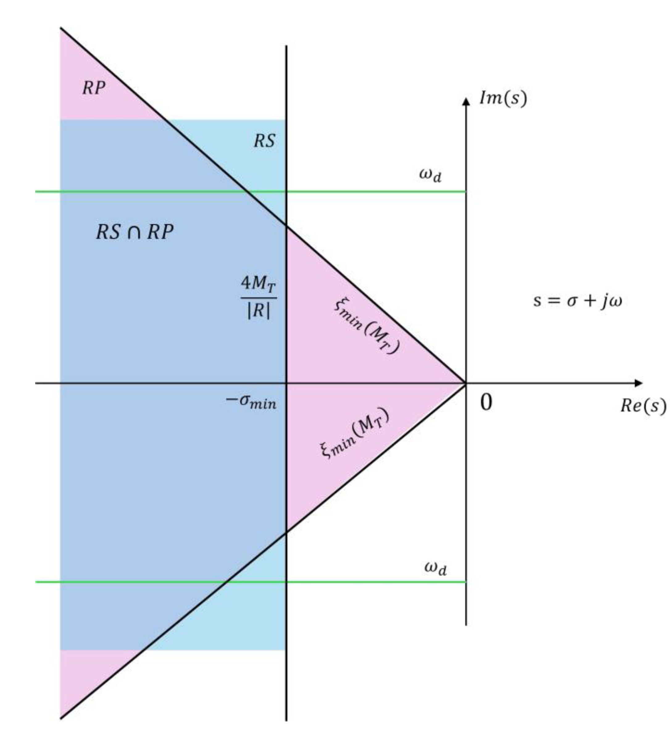
Figure 9 illustrates the geometric interpretation of the constraints induced by the circular condition (17) in the s-plane and based on (73)–(75). The light blue region represents the admissible area defined by robust stability $RS$, determined by the minimum horizontal distance $\mathrm{R}\mathrm{e}\left\{s\right\}\le -{\sigma }_{\mathrm{m}\mathrm{i}\mathrm{n}}$. The inclined boundaries forming the wedge-shaped pink region correspond to the minimum damping condition $\xi \ge {\xi }_{\mathrm{m}\mathrm{i}\mathrm{n}}(M_T)$ and determine the admissible overshoot of the closed-loop control system. The overlapping purple region shows the set of dominant closed-loop pole locations for which the requirements on both speed of response and overshoot, derived from the considered frequency domain circular constraint (17), are simultaneously satisfied.

The requirement for a maximum admissible overshoot of the closed-loop system (76) leads to a lower bound on the damping ratio $\xi$, which follows directly from the classical relation between ${\sigma }_{,\mathrm{\%}}$ and $\xi$, given in (72), and can be written in the form (77).

$${\sigma ,}_{\mathrm{\%}}\le {{\sigma }_{,\mathrm{\%}}}^{\mathrm{m}\mathrm{a}\mathrm{x}}$$

(76)

$$\xi \ge {\xi }_{\mathrm{m}\mathrm{i}\mathrm{n}}\left({{\sigma ,}_{\mathrm{\%}}}^{\mathrm{m}\mathrm{a}\mathrm{x}}\right).$$

(77)

Condition (77) defines a wedge-shaped admissible region in the s-plane, bounded by straight lines forming a constant angle with respect to the negative real axis, as illustrated in Figure 9.

In an equivalent geometric form, using the relationship between the parameters of the dominant dynamics, inequality (77) can be written as an angular constraint (78).

$$\left|{\omega }_d\right|\le \sigma \sqrt{{\displaystyle \frac{1}{{\xi }_{\mathrm{m}\mathrm{i}\mathrm{n}}}}-1},$$

(78)

which determines admissibility along the ${\omega }_d$ axis, visualized in green in Figure 9.

It should be emphasized that the ${\omega }_d$ constraint (78), shown by the green lines in Figure 9, is not an additional independent condition, but an equivalent representation of the angular constraint $\xi \ge {\xi }_{\mathrm{m}\mathrm{i}\mathrm{n}}$, i.e., of $RP$. In this way, the requirement for limited overshoot is interpreted as a purely geometric condition in the s-plane, without the need for a direct reference to the transient response of the system.

The combination of the circular constraint in the frequency domain for robust stability $RS$, defined by (17) and interpreted geometrically through the minimum horizontal distance (66), and the requirement for limited overshoot $RP$, formulated by (76) and equivalent to the angular constraint (77), (78), leads to a system of geometric conditions for the location of the dominant closed-loop poles in the s-plane (79).

$$\left\{\begin{array}{c}\sigma \ge {\sigma }_{\mathrm{m}\mathrm{i}\mathrm{n}}\left(M_T\right),\\ \xi \ge {\xi }_{\mathrm{m}\mathrm{i}\mathrm{n}}\left({\sigma ,}_{\%}\right)\end{array}\right.$$

(79)

where ${\sigma }_{\mathrm{m}\mathrm{i}\mathrm{n}}(M_T)$ is defined in (66), and ${\xi }_{\mathrm{m}\mathrm{i}\mathrm{n}}({\sigma ,}_{\mathrm{\%}})$ in (77).

Geometrically, this means that the admissible locations of the dominant poles are determined as the intersection of the regions associated separately with the conditions $RS$and $RP$. Robust stability $RS$ manifests geometrically as a requirement for a minimum horizontal distance of the dominant poles from the imaginary axis, ${\sigma }_{\mathrm{m}\mathrm{i}\mathrm{n}}$, while robust performance $RP$ manifests through an angular constraint associated with the minimum damping ratio ${\xi }_{\mathrm{m}\mathrm{i}\mathrm{n}}$ and limited overshoot.

System (79) defines a combined admissible region in the s-plane, obtained as the intersection of the vertical boundary $\sigma ={\sigma }_{\mathrm{m}\mathrm{i}\mathrm{n}}$, derived from the frequency domain requirement for robust stability (blue), and the wedge-shaped region determined by the minimum damping ratio ${\xi }_{\mathrm{m}\mathrm{i}\mathrm{n}}$(pink).

The overlapping purple region in Figure 9 represents precisely the combined admissible set $RS\cap RP$.

The blue region reflects the constraint $\sigma \ge {\sigma }_{\mathrm{m}\mathrm{i}\mathrm{n}}$ from (66), the pink wedge-shaped region corresponds to the condition $\xi \ge {\xi }_{\mathrm{m}\mathrm{i}\mathrm{n}}$ given in (77), and the overlapping purple region represents the combined admissible set $RS\cap RP$. The green horizontal lines show the equivalent representation of condition (78) along the ${\omega }_d$ axis.

While in the s-plane the dominant dynamics is described through the real and imaginary parts of the poles $\left(\sigma ,{\omega }_d\right)$, for the purposes of performance analysis and design it is more convenient to parameterize the same dynamics using the damping ratio $\xi$ and the undamped natural frequency ${\omega }_n$.

The two representations are equivalent to dominant second-order dynamics and are related through the relations $\sigma =\xi {\omega }_n$ and ${\omega }_d={\omega }_n\sqrt{1-{\xi }^2}$. From the combined geometric conditions for robust stability and limited overshoot, formulated by (66), (77), and system (79), an explicit lower bound on the undamped natural frequency of the closed-loop control system follows (80).

$${\omega }_n\ge {\omega }_{n,\mathrm{m}\mathrm{i}\mathrm{n}}={\displaystyle \frac{{\sigma }_{\mathrm{m}\mathrm{i}\mathrm{n}}}{{\xi }_{\mathrm{m}\mathrm{i}\mathrm{n}}}},$$

(80)

where ${\sigma }_{\mathrm{m}\mathrm{i}\mathrm{n}}$ is defined in (66), and ${\xi }_{\mathrm{m}\mathrm{i}\mathrm{n}}$ in (77).

Bound (80) follows directly from the relation ${\omega }_n=\sigma /\xi$, valid for dominant second-order dynamics, and from the combined conditions $\sigma \ge {\sigma }_{\mathrm{m}\mathrm{i}\mathrm{n}}$ and $\xi \ge {\xi }_{\mathrm{m}\mathrm{i}\mathrm{n}}$.

Inequality (80) defines the projection of the combined admissible region $RS\cap RP$ onto the parameter space $\left(\xi ,{\omega }_n\right)$, which can be described by the set (81).

$${\mathcal{A}}_{\left(\xi ,,{\omega }_n\right)}=\left\{(\xi ,{\omega }_n)\in {\mathbb{R}}^2:\xi \ge {\xi }_{\mathrm{m}\mathrm{i}\mathrm{n}}, {\omega }_n\ge {\displaystyle \frac{{\sigma }_{\mathrm{m}\mathrm{i}\mathrm{n}}}{\xi }}\right\}.$$

(81)

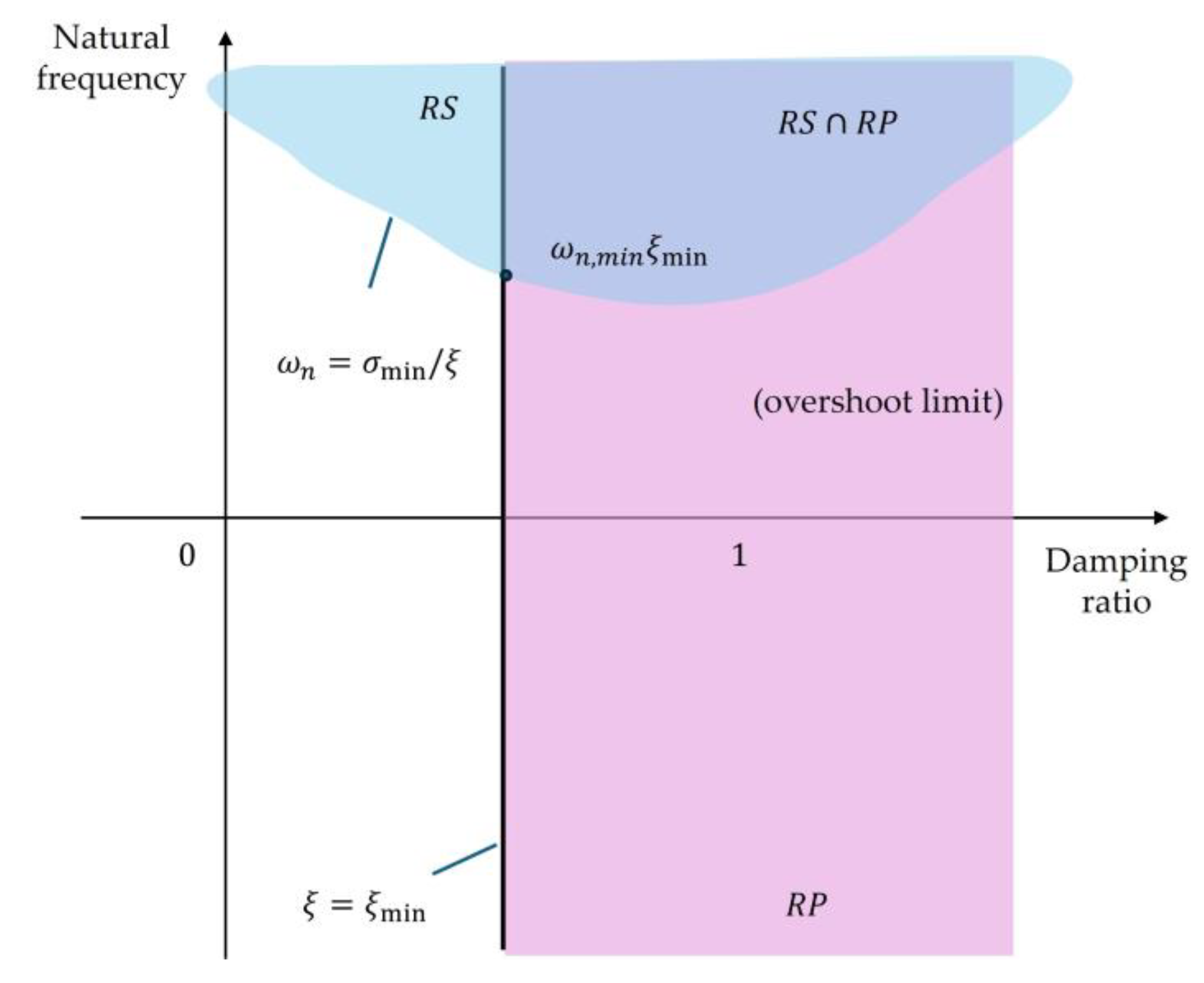
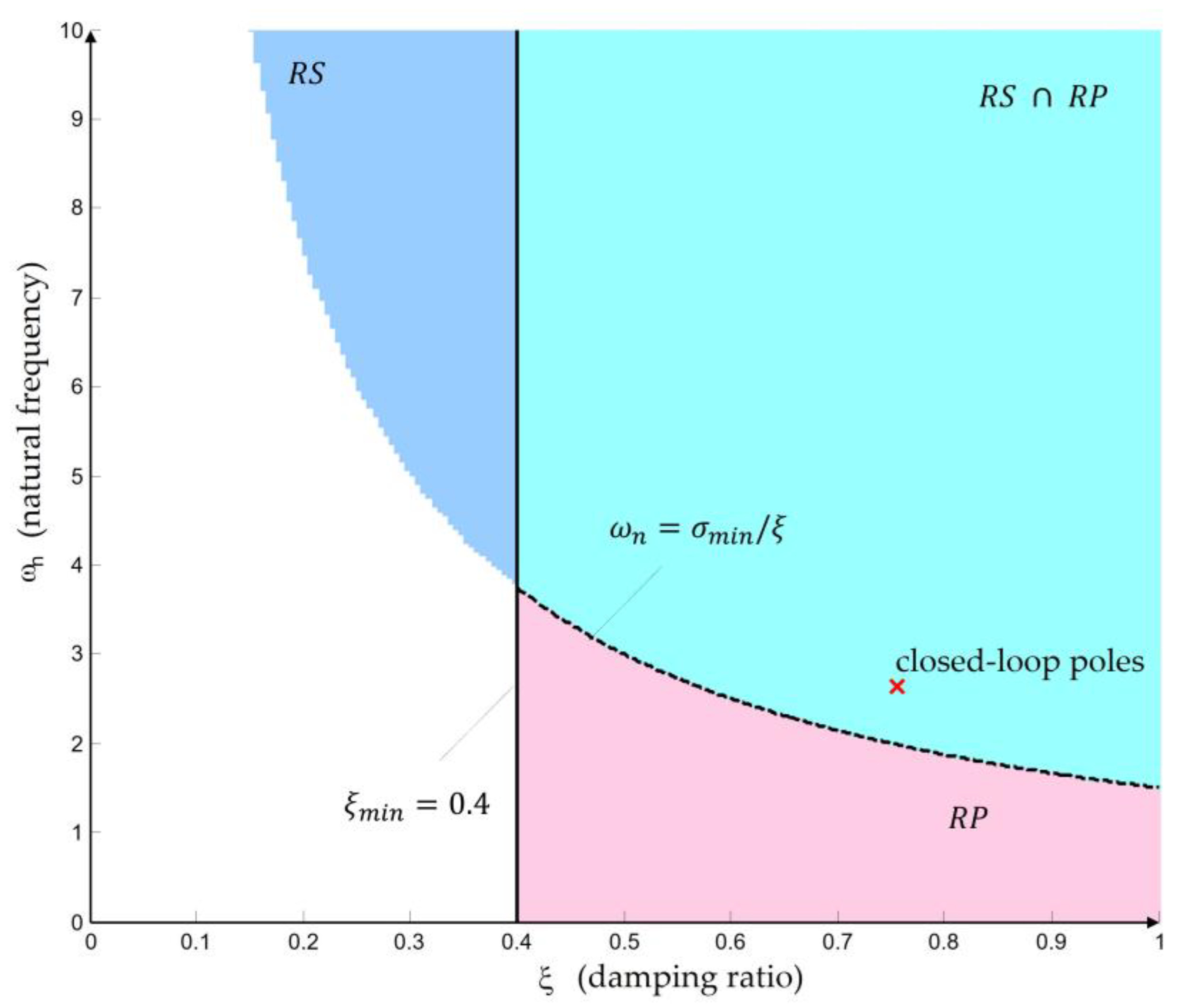
Geometrically, the set ${\mathcal{A}}_{\left(\xi ,,{\omega }_n\right)}$ represents an admissible design region in the parameter space of the dominant dynamics, within which the requirements for robust stability and limited overshoot are simultaneously satisfied, as shown in Figure 10. In this way, the robustness constraints defined in the frequency domain are translated into direct conditions on the parameters $\xi$ and ${\omega }_n$, allowing the design problem to be formulated as the selection of parameters within an admissible region, without the need for iterative frequency or time domain analysis.

The vertical boundary $\xi ={\xi }_{\mathrm{m}\mathrm{i}\mathrm{n}}$ follows from the constraint on the maximum allowable overshoot, while the nonlinear boundary ${\omega }_n={\sigma }_{\mathrm{m}\mathrm{i}\mathrm{n}}/\xi$ is the projection of the vertical boundary $\mathrm{R}\mathrm{e}\left\{s\right\}=-{\sigma }_{\mathrm{m}\mathrm{i}\mathrm{n}}$ in the root plane. The shaded region defines all combinations $\left(\xi ,{\omega }_n\right)$ that guarantee simultaneous satisfaction of the requirements for robust stability, robust performance, and the corresponding direct performance indicators related to speed of response.

The circular constraints in the frequency domain, used for robust stability and robust performance, impose not only frequency domain conditions but also specific numerical bounds on the direct performance indicators of the closed-loop control system. These constraints lead to explicit estimates for the maximum overshoot, the minimum speed of transient response through the settling time, as well as for the admissible values of the dominant dynamics parameters ${\omega }_n$ and $\xi$.

5. Example and Discussion

This section presents a numerical validation of the results from Section 4. The considered example illustrates how the frequency domain constraints, formulated as circular sets in the Nyquist plane according to (8), (10)–(12), and (17), induce admissible and forbidden geometric regions in the s-plane through the preimage transformation (5).

The obtained bounds are interpreted through relations (66) and (77)–(79), demonstrating how the frequency domain robustness requirements lead to explicit constraints on the location of the dominant closed-loop poles.

In particular, the example shows how the imposed circular constraints determine the critical frequencies ${\omega }^{*}$, the active boundaries, the admissible regions for the dominant poles, and the corresponding direct performance indicators in the transient response, including settling time and overshoot, in accordance with (72)–(75).

5.1. Description of Example and Dominant Dynamics

An open-loop system is considered with transfer function $W(s)={\displaystyle \frac{K_p}{\left(s+1)(s+3\right)}},K_p=4.$ Under unity negative feedback, the closed-loop transfer function becomes $T(s)={\displaystyle \frac{W(s)}{1+W(s)}}={\displaystyle \frac{4}{s^2+4s+7}}.$ The main parameters of the example considered are summarized in Table 1. These values are used as reference in the interpretation of the frequency domain and geometric constraints in the following subsections, as well as in the analysis of the performance indicators, including overshoot and settling time.

The frequency domain constraints used in the analysis are summarized in Table 2 and will be applied sequentially in the discussion that follows.

5.2. Circular Sets in the Nyquist Plane of Sensitivity and Complementary Sensitivity

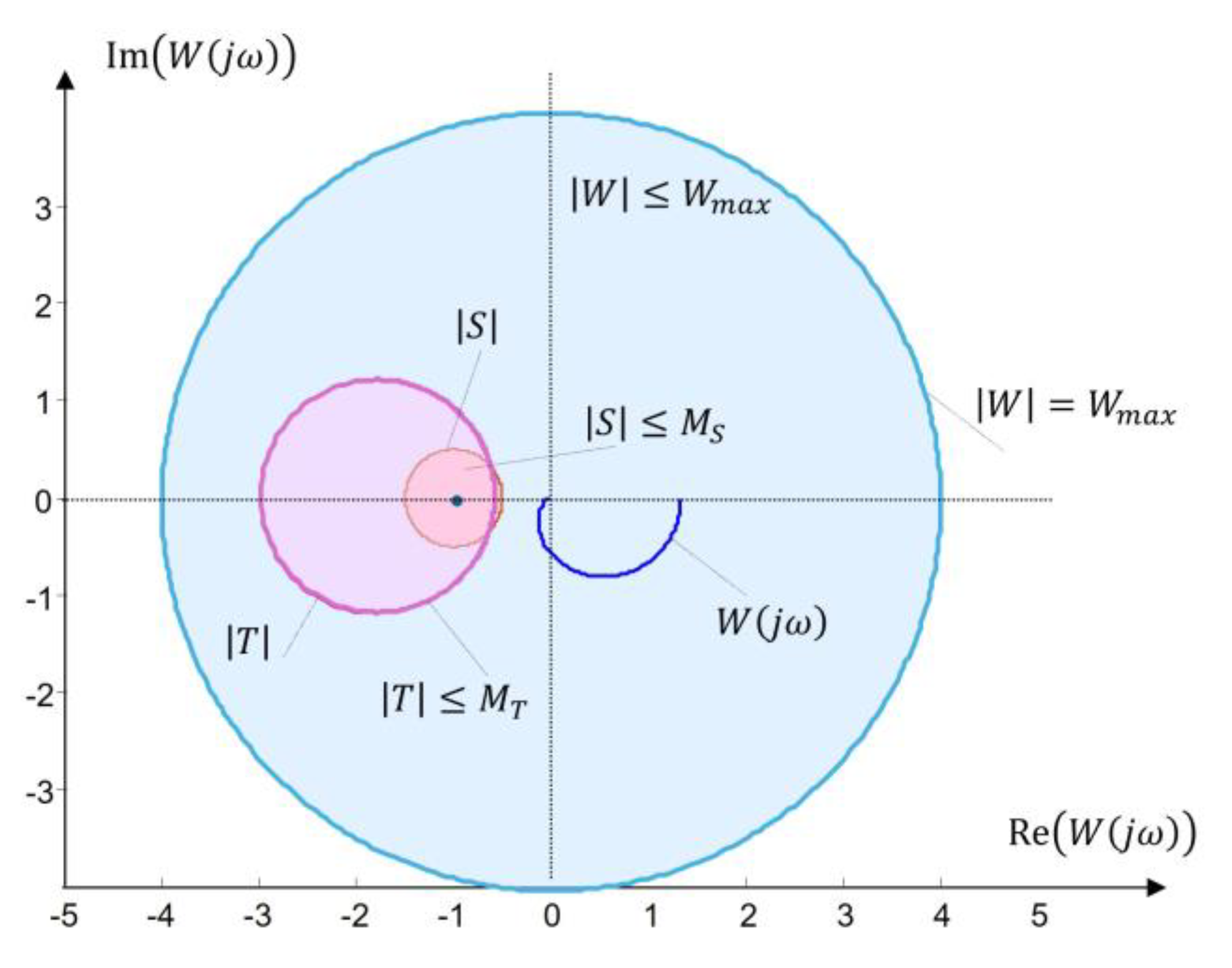
Figure 11 shows the Nyquist locus of the open-loop system $W(j\omega )$ together with the circular sets generated by the frequency domain constraints. The parameters of the constraints are given in Table 2.

The constraint on sensitivity, formulated through (11), leads to a circular forbidden region around the critical point $-1$. According to the fractional-linear relation (7) and the geometric interpretation (10), (11), the condition on $S(j\omega )$ is represented as a circle in the Nyquist plane, with the admissible region being its exterior. For the considered system, the minimum distance of the frequency response to the critical point is $\underset{\omega }{\mathrm{m}\mathrm{i}\mathrm{n}}\left|1+W(j\omega )\right|\approx 0.63,$ with the minimum attained at the critical frequency ${\omega }_S^{\star }\approx 2.6\mathrm{rad}/\mathrm{s}.$ This shows that the sensitivity constraint is active but not violated.

Similarly, the constraint on complementary sensitivity, introduced through (17), induces an isomodular boundary in the Nyquist plane via transformation (7) and its equivalent circular representation (12), (13). For the considered control system, due to the damping ratio value $\xi \approx 0.756>1/\sqrt{2}$, no resonance peak of $\left|T\left(j\omega \right)\right|$is observed. Therefore, the maximum of the complementary sensitivity is attained at $\omega =0$ and equals $\left|T\left(j0\right)\right|=1.$ Thus, $\underset{\omega }{\max }\left|T\left(j\omega \right)\right|=1<M_T=1.5,$ which means that the complementary sensitivity constraint is not active and is satisfied with margin. Consequently, the sensitivity constraint is active, while the complementary sensitivity constraint is satisfied with reserve. Figure 11 shows that the frequency response remains outside the corresponding forbidden regions, confirming the geometric interpretation of the constraints derived analytically in Section 4 and preparing the transition to the analysis in the s-plane.

5.3. Circular Interpretation of Gain and Phase Margins in the Nyquist Plane

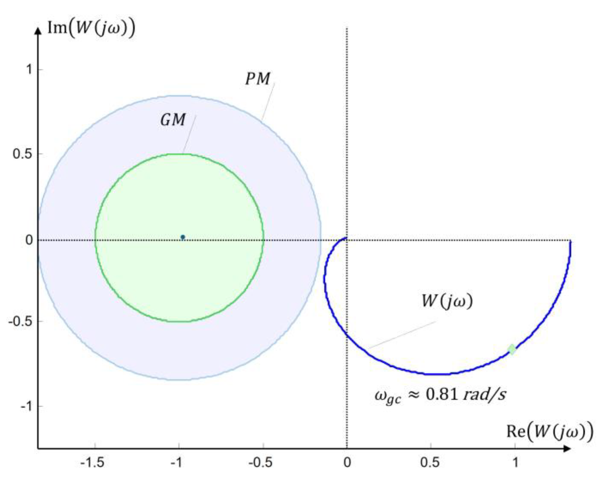
A requirement for a minimum phase margin of the form (29) with $PM\ge {50}^{\circ }$is imposed. For the system considered, the actual phase margin is approximately $PM\approx {125.9}^{\circ }$ at the gain crossover frequency ${\omega }_{gc}\approx 0.81\mathrm{rad}/\mathrm{s},$ which significantly exceeds the specified requirement. According to the geometric interpretation in (30), the phase margin condition leads to a constraint of the form $\left|1+W(j\omega )\right|\ge r_{PM},$ where $r_{PM}=2\mathrm{s}\mathrm{i}\mathrm{n}\left({\displaystyle \frac{{\phi }_m}{2}}\right),$ which defines the exterior of a circle centered at the critical point $-1$ in the Nyquist plane. The frequency response $W(j\omega )$ remains outside this circle, with the point at ${\omega }_{gc}$ being critical (boundary) for the definition of the phase margin, as shown in Figure 12.

The gain margin $GM$ for the system considered is infinite, since the phase of the frequency response does not reach the value $-\pi$ at any finite frequency. A requirement for a minimum gain margin of the form (23) with $GM\ge 2$ is introduced. According to the equivalent geometric condition (24), this requirement also leads to a circular constraint of the form $\left|1+W(j\omega )\right|\ge r_{GM},$ where $r_{GM}={\displaystyle \frac{g-1}{g}},$ which again defines the exterior of a circle centered at $-1$, shown in Figure 13. It should be emphasized that the gain and phase margins, although they admit a geometric interpretation through circular constraints, represent frequency local conditions (at ${\omega }_{gc}$ and ${\omega }_{-\pi }$) and do not form a frequency-dependent family of circles. For this reason, they do not participate in the formation of the active geometric envelope. The reason is that they represent frequency local and fixed constraints, in contrast to the frequency-dependent circles $C_S(\omega )$ and $C_T(\omega )$, which determine the active boundary of the admissible region.

5.4. Frequency Dependent Circular Sets and Formation of the Active Envelope

In the general case, constraints of the form (11) and (17) may be frequency dependent, i.e., $M_S=M_S(\omega )$ and $M_T=M_T(\omega )$. According to the geometric construction formulated in (55), (56), this leads to families of circular sets $C_S(\omega )$ and $C_T(\omega )$ in the Nyquist plane, parameterized by frequency. For each fixed frequency $\omega$, the corresponding constraint induces a separate circle, so that instead of a single circular set, a continuous family of circles is obtained. The same basic constraints introduced in Table 2 are used, extended to the frequency dependent case. The admissible region is obtained as the intersection of the exteriors of all $C_S(\omega )$ and the interiors of all $C_T(\omega )$, and its boundary forms an active geometric envelope.

In the considered example, frequency dependent bounds $M_S(\omega )$ and $M_T(\omega )$ are used, with an additional condition $M_T(\omega )<1$. Numerically, this is implemented by imposing $M_T(\omega )\le 0.9$, which guarantees that the sets $C_T(\omega )$ are of the type defined in (12), (13). This is done to demonstrate an “interior” type constraint. Since $M_T(\omega )<1$, the corresponding circles are interior admissible sets and constrain the frequency response “from inside”, in contrast to the sensitivity constraints, which act as exterior forbidden regions around the critical point −1. The radii and centers of the corresponding circular sets are determined according to (12), (13), and for $C_S(\omega )$ according to (10), (11).

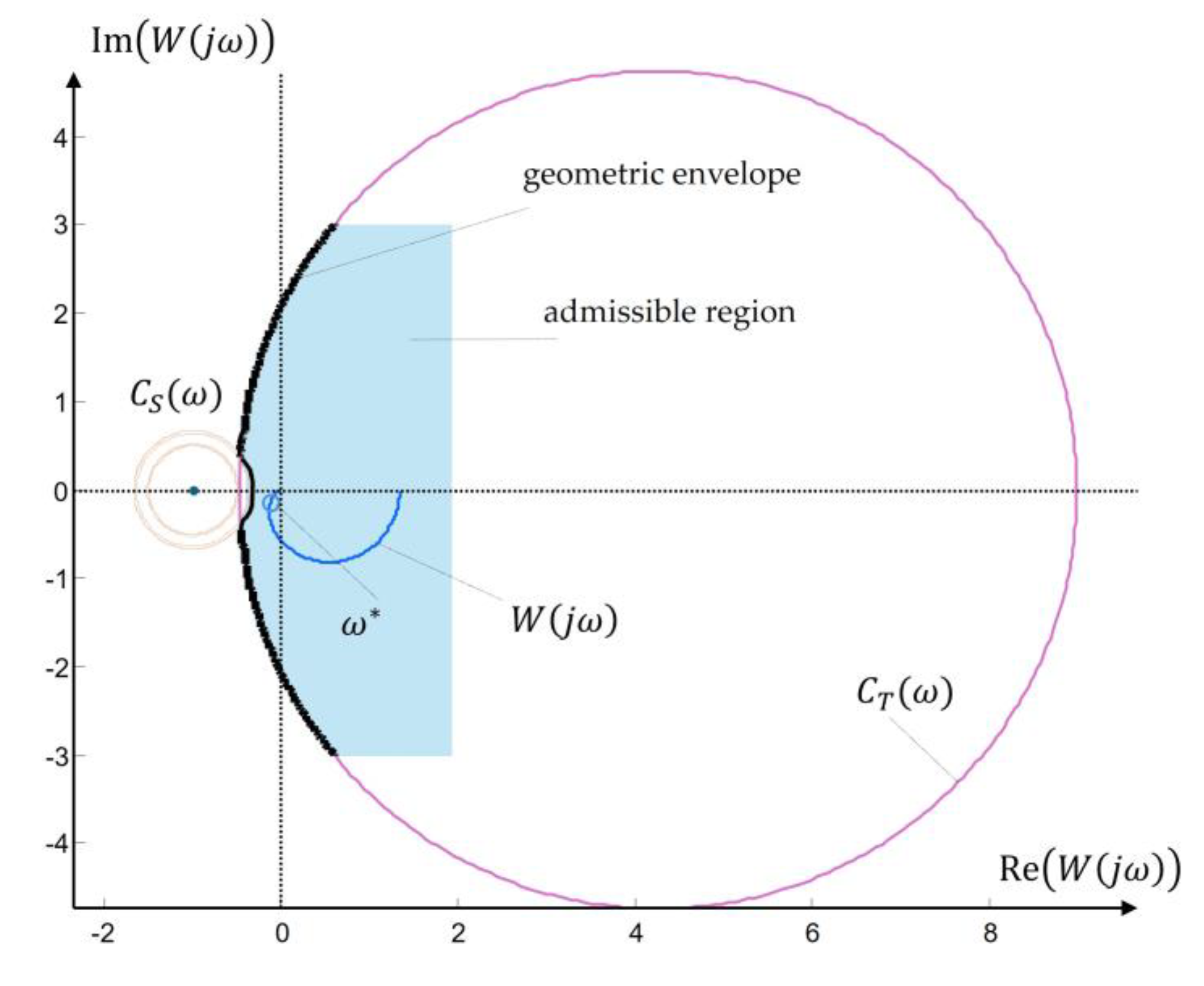
Figure 13 shows the intersection of all these constraints in the Nyquist plane. The light gray region represents the admissible set, and the solid black curve is a numerical approximation of the active geometric envelope. This envelope represents the geometric set of points at which one of the frequency-depending constraints becomes active, i.e., satisfied with equality. The dashed blue and purple circles illustrate individual representatives of the families $C_S(\omega )$ and $C_T(\omega )$. The frequency response of the open loop controlsystem $W(j\omega )$ lies entirely inside the admissible region.

The closest approach to the active boundary occurs at a frequency ${\omega }^{\star }$, defined as the frequency at which one of the combined constraints becomes active. This means that at ${\omega }^{\star }$, the open loop frequency response is tangent to a corresponding circle from the family and locally determines the geometry of the envelope. For the considered example, it is numerically obtained that ${\omega }^{\star }\approx 2\text{–}3\mathrm{rad}/\mathrm{s}$, which coincides with the frequency range of maximum sensitivity and resonance of the closed-loop control system (see Table 1). This frequency determines the active point of the geometric envelope.

Therefore, frequency dependent constraints do not lead to separate local circles, but to a geometric structure an active geometric envelope which represents the boundary of the admissible set in the Nyquist plane and generalizes the local frequency constraints from (11) and (17). In this sense, the worst-case behavior is determined not by a single circle, but by the collection of active arcs at different frequencies.

5.5. Robust Stability and Robust Performance as Circular Sets in the Nyquist Plane

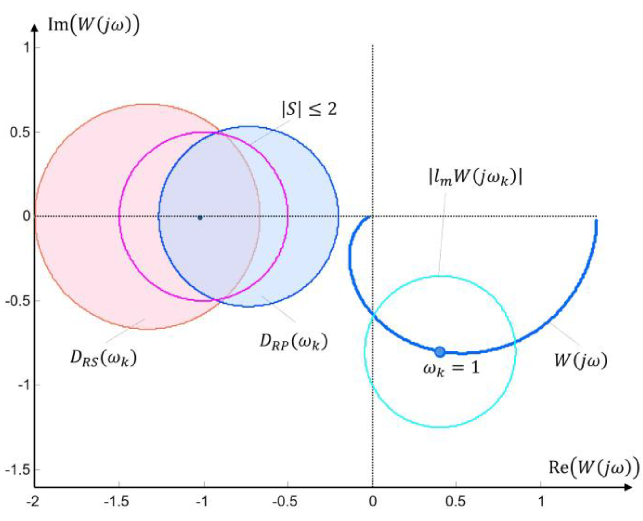
Figure 14 presents the geometric interpretation of the conditions for robust stability and robust performance, formulated by (57) and (58), respectively, for a fixed frequency ${\omega }_k=1\mathrm{rad}/\mathrm{s}$. At this frequency, the open-loop control system takes the value $W(j{\omega }_k)=0.40-j0.80$, which is consistent with the dynamic parameters of the system given in Table 1. According to (57), the robust stability condition defines a circular admissible set $D_{RS}({\omega }_k)$ in the Nyquist plane. For a given multiplicative uncertainty $\left|l_m(j{\omega }_k)\right|=0.5$ (see Table 2), the local circle is centered at $W(j{\omega }_k)$and has radius $\left|l_{m}W(j{\omega }_k)\right|$ which determines the maximum admissible local variation while preserving stability.

The robust performance condition, introduced by (58), leads to a stricter admissible set $D_{RP}({\omega }_k)$, nested inside $D_{RS}({\omega }_k)$ according to (59). Due to the presence of the additive term $y^0(j{\omega }_k)S(j{\omega }_k)$, the center of the corresponding circular constraint is shifted, which geometrically appears as a smaller and oriented admissible region around the operating point. The numerical values show that the $RP$ constraint becomes active earlier than the$RS$ constraint, confirming the stricter nature of robust performance.

Figure 14 also shows the S-circle resulting from the global constraint $\left|S(j\omega )\right|\le M_S$, introduced in Table 2 and defined geometrically by (10), (11). This circle represents a global frequency constraint with center at the critical point −1 and radius $1/M_S$, limiting the minimum admissible distance of the frequency response $W(j\omega )$ from −1. The combination of the three constraints, the global S-circle, the local multiplicative circle $\left|l_{m}W\right|$ and the nested sets $D_{RP}({\omega }_k)\subset D_{RS}({\omega }_k)$ provides a complete geometric picture of robustness. Figure 14 visualizes the position of $W(j{\omega }_k)$, the local admissible variation, and the interaction between the global sensitivity constraints and the local robustness conditions.

Thus, the geometric sets defined by (10), (11) and (57), (58) are presented as a unified system of circular constraints, enabling simultaneous assessment of stability, sensitivity, and robust performance at a selected frequency.

5.6. Preimage of Circular Constraints in the Root Plane

In accordance with the geometric construction formulated in (55), (56), the circular sets in the Nyquist plane generated by the constraints on sensitivity and complementary sensitivity can be transferred to the s-plane through the preimage transformation (7).

In this way, each point $s=\sigma +j\omega$ can be classified as admissible or inadmissible with respect to the constraints $\left|S(s)\right|\le M_{S }$ and $\left|T(s)\right|\le M_T$, which in the Nyquist plane realize the circular sets (10)–(12) and (17). The resulting region represents the preimage of these constraints and determines the admissible locations of the closed loop poles. In the numerical analysis, the constraints $\left|S(s)\right|\le M_{S }$ and $\left|T(s)\right|\le M_T$ introduced in Table 2, are used.

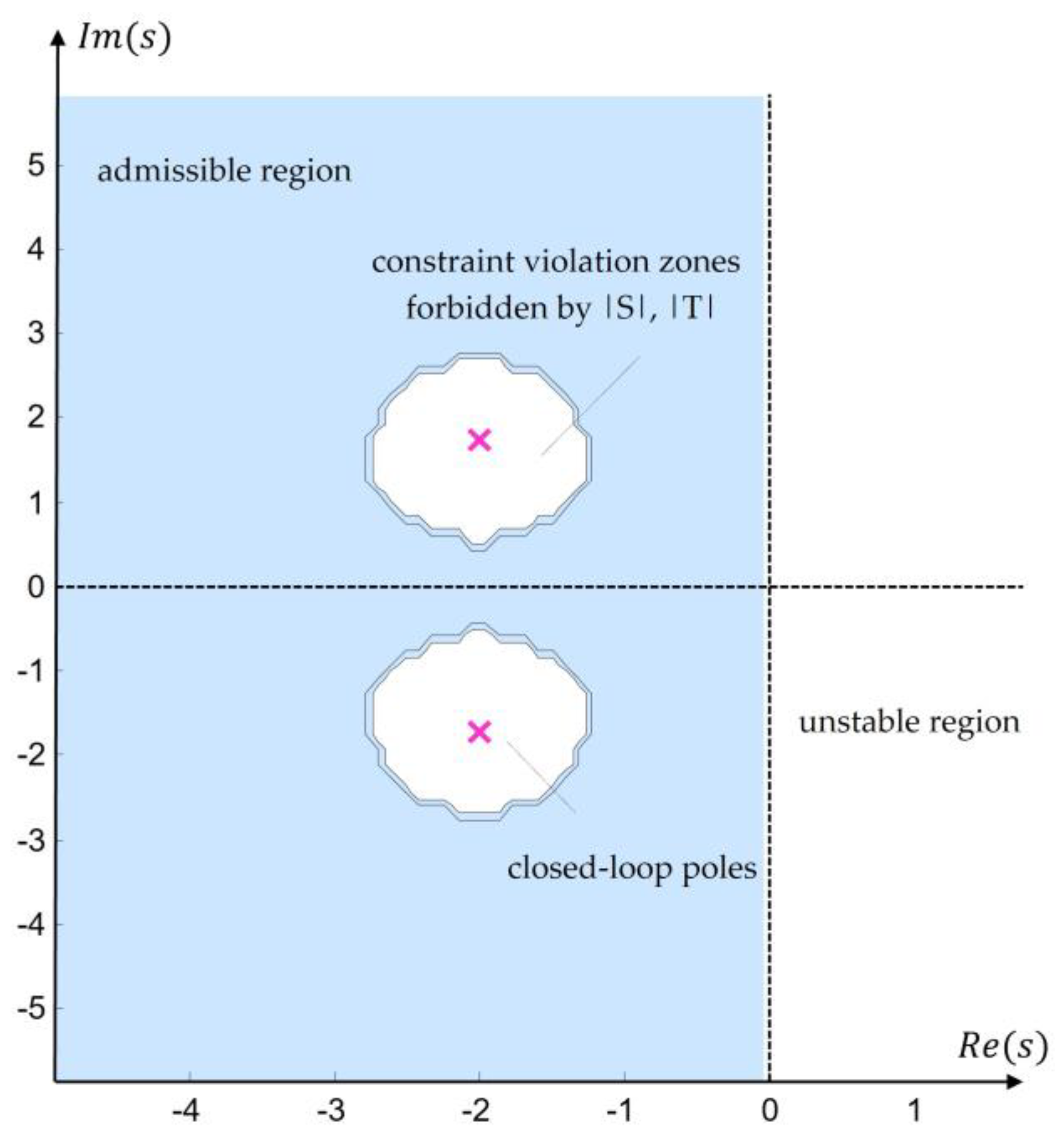
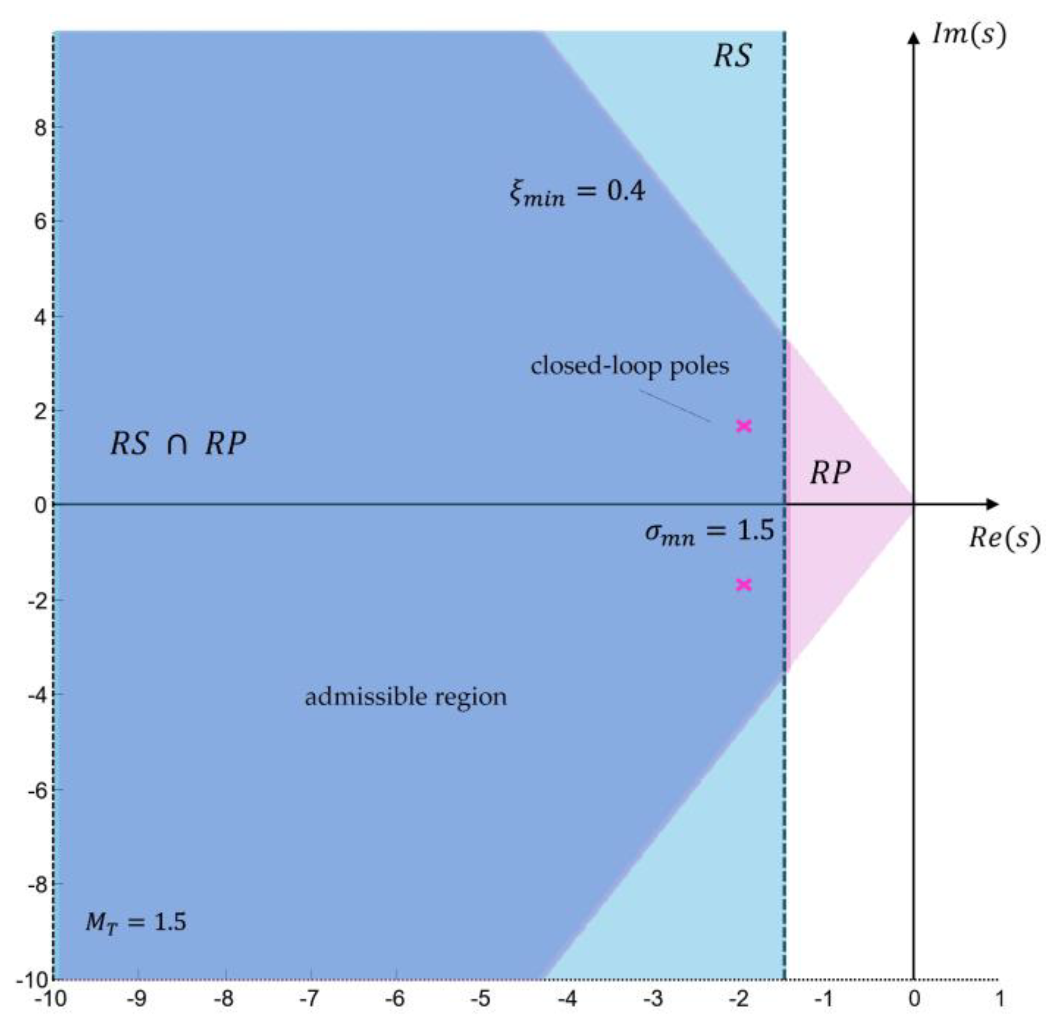
A grid approximation of the complex region $\sigma \in [-\mathrm{10,0}],$ $\omega \in [-\mathrm{10,10}]$ allows direct evaluation of $S(s)$ and $T(s)$ via (7). The resulting admissible region represents the preimage of the corresponding circular sets in the Nyquist plane. The graphical result (Figure 15) shows a compact region located in the left half-plane that contains the dominant closed-loop poles $p_{\mathrm{1,2}}=-2\pm j\sqrt{3}$, given in Table 1. This confirms the consistency between the frequency domain constraints and the actual control system dynamics. The admissible region describes all points in the s-plane for which the sensitivity and complementary sensitivity constraints are simultaneously satisfied and thus represents a geometric analogue of the closed-loop operating region determined through (72)–(75).

Therefore, the preimage of the frequency circular constraints transforms the limitations in the Nyquist plane into admissible and forbidden regions in the s-plane. The light blue region in Figure 15 represents the admissible zone obtained as the preimage of the frequency constraints, while the white regions denote violation zones of either the $\left|S\right|$ or $\left|T\right|$constraints. The resulting compact light blue region in the left half-plane contains the dominant closed-loop poles of the control system, confirming the consistency between the frequency specifications and the actual dynamics. Any pole located in the white region leads to violation of at least one of the imposed constraints.

Thus, the geometry of admissible pole locations follows directly from the frequency formulated robustness requirements.

5.7. Admissible Regions in the s-plane

The frequency conditions for robust stability and robust performance introduced in the previous subsections induce admissible regions for the location of the dominant closed-loop poles, determined by the constraints in Table 2 and the dynamic parameters in Table 1. According to the relationship between the resonance peak and the damping ratio (20), the constraint on complementary sensitivity leads to a lower bound on the damping ratio $\xi \ge 0.357$. Since this condition is weaker than the imposed requirement ${\xi }_{\mathrm{m}\mathrm{i}\mathrm{n}}=0.4$, the active robust performance constraint in the example is $\xi \ge 0.4$, which defines a wedge-shaped admissible region bounded by straight lines with constant angle with respect to the negative real axis, in accordance with (77), (78).

The robust stability constraint introduces an additional bound on the real part of the poles of the form $\mathrm{R}\mathrm{e}\left\{s\right\}\le -{\sigma }_{\mathrm{m}\mathrm{i}\mathrm{n}}$, obtained from the local estimate (66). For the selected value ${\sigma }_{\mathrm{m}\mathrm{i}\mathrm{n}}=1.5$, this boundary allows slower dynamics compared to the nominal dominant closed-loop poles (see Table 1) and corresponds to a maximum settling time of approximately $t_s\approx 4/{\sigma }_{\mathrm{m}\mathrm{i}\mathrm{n}}\approx 2.7\mathrm{s}$, according to (73).

The intersection of the wedge-shaped region $RP$ and the vertical boundary $RS$ forms the combined admissible region $RS\cap RP$, defined by the control system of conditions (79). Figure 16 shows this region in the s-plane, where the dominant poles of the considered control system lie entirely inside it. This confirms the consistency between the frequency constraints and the actual closed-loop dynamics.

In this way, the geometric approach provides a direct connection between frequency constraints on sensitivity and robustness and the time domain performance indicators of the closed-loop system, allowing a clear interpretation of the admissible pole locations in the s-plane. Robust stability and robust performance result in a geometric region defined as the intersection of time-related (${\sigma }_{\mathrm{m}\mathrm{i}\mathrm{n}}$) and dynamic (${\xi }_{\mathrm{m}\mathrm{i}\mathrm{n}}$) constraints.

5.8. Projection of the Combined Constraints onto the Parameter Space $\left(\xi ,{\omega }_n\right)$

The projection onto the parameter space $\left(\xi ,{\omega }_n\right)$ provides a natural link between the geometric constraints on the pole locations and the classical performance indices of the closed-loop control system. Through the transformation from the s-plane to the second-order parameters, a direct interpretation of the frequency constraints in terms of damping ratio and natural frequency is obtained.

The geometric boundaries derived in the previous subsections lead to two main constraints in the $\left(\xi ,{\omega }_n\right)$-space. The first arises from the lower bound on the real part of the poles, defined by (66), and appears as a hyperbolic boundary of the form ${\omega }_n={\sigma }_{\mathrm{m}\mathrm{i}\mathrm{n}}/\xi$. The second constraint is associated with the minimum admissible damping ratio and defines a vertical boundary $\xi ={\xi }_{\mathrm{m}\mathrm{i}\mathrm{n}}$, according to (77), (78). These two conditions represent the parametric counterpart of the robust stability and robust performance constraints introduced in Table 2.

The intersection of these two boundaries forms the admissible design region in the $\left(\xi ,{\omega }_n\right)$-space, which can be regarded as the parametric equivalent of the combined region $RS\cap RP$ in the s-plane. Figure 17 illustrates this projection, where the actual parameter values of the dominant closed-loop poles (see Table 1) lie entirely within the admissible region.

This interpretation enables a direct connection between frequency constraints and time domain performance indices. The minimum value of $\xi$ guarantees limited overshoot, while the bound on ${\sigma }_{\mathrm{m}\mathrm{i}\mathrm{n}}$ ensures a constraint on the settling time. In this way, the projection onto the $\left(\xi ,{\omega }_n\right)$-space unifies frequency domain and time domain analysis, providing an intuitive tool for assessing the performance of the closed-loop control system.

5.9. Discussion

A key conclusion from the presented example is that frequency domain constraints can be interpreted as geometrically defined admissible and forbidden regions in the complex plane. Constraints of the form $\left|S\right|\le M_S$ and $\left|T\right|\le M_T$ induce circular forbidden regions in the Nyquist plane, which directly restrict the admissible shape of the frequency response of the open-loop control system $W(j\omega ).$In practical terms, this means that a small number of scalar constraints on sensitivity and complementary sensitivity lead to global geometric restrictions on system behavior. These constraints can be transferred via the preimage into the s-plane and interpreted as admissible regions for the pole locations, and subsequently as regions in the parametric space $\left(\xi ,{\omega }_n\right)$ of the dominant closed-loop dynamics.

From an engineering perspective, this allows complex frequency requirements to be viewed as forbidden regions in different system representations. Thus, already at the level of selecting boundary values for $M_S$ and $M_T$, an intuitive and quantitative understanding of the admissible dynamics can be obtained, without the need for a complete frequency analysis.

This interpretation highlights the practical value of the geometric approach, as it translates frequency constraints into easily visualizable regions that can be used directly in the analysis and design of robust control systems.

The presented study demonstrates the geometric mechanism through which frequency domain constraints, formulated via modulus inequalities, generated circular admissible sets in the Nyquist plane and, through their preimage, induce admissible regions in the s-plane. It has been shown that classical robustness measures (gain margin, phase margin, sensitivity and complementary sensitivity constraints) can be treated as cases of a unified class of circular geometric constraints. Furthermore, a direct connection has been established between these frequency-formulated constraints and the time domain performance indices of the closed-loop control system, allowing them to be interpreted as geometric consequences in the s-plane and in the parametric space.

In this way, the proposed geometric approach not only interprets but also structures the relationship between robust analysis in the frequency domain and time domain performance indices, unifying them within a single analytical framework.

6. Conclusions

A geometric approach for the analysis of frequency domain constraints has been proposed, based on their representation as circular sets in the Nyquist plane of the open-loop control system. A unified geometric mechanism has been systematized, through which constraints on sensitivity and complementary sensitivity, as well as classical gain and phase margins, are treated as cases of a common class of circular constraints generated by fractional-linear transformations. It has been shown that sensitivity and complementary sensitivity constraints, together with gain and phase margins, admit a unified geometric interpretation via fractional-linear transformations, and that under combined frequency-dependent constraints the actual boundary of admissible behavior is determined by an active geometric envelope that generalizes the local frequency conditions.

The practical value of the proposed approach lies in the fact that abstract robust requirements formulated in the frequency domain are translated into clear geometric constraints, enabling direct assessment of admissible system behavior and of the available margin before violation of the imposed requirements. Through the preimage mapping into the s-plane, a direct geometric relationship has been established between formulated robust conditions in frequency domain and the admissible locations of the dominant closed-loop poles. This further implies a direct connection with time domain performance indices, allowing robustness to be evaluated already at the analysis stage, without the need for additional time domain simulations or active experimental validation.

A limitation of the study is that it is formulated within the framework of linear time-invariant systems. In this sense, its applicability to nonlinear systems requires further development of the geometric approach and the corresponding preimage constructions, which outlines a natural direction for future research. Additionally, the presented geometric interpretation has been developed in the context of single-input single-output control systems. Its extension to multivariable structures requires the use of more complex geometric objects and generalized robustness measures.

The proposed research can be used both for the analysis of existing control systems and as a foundation for controller design with predefined robust requirements. The approach provides guidance for shaping the frequency response and for selecting admissible parameters of the dominant dynamics, naturally complementing both classical and robust analysis and design methods.

References

1. Morari, M.; Zafiriou, E. Robust Process Control; Prentice Hall: Englewood Cliffs, NJ, USA, 1989. [Google Scholar]
2. Doyle, J.C.; Francis, B.A.; Tannenbaum, A.R. Feedback Control Theory; Macmillan Publishing Co.: New York, NY, USA, 1992. [Google Scholar]
3. Vidyasagar, M. Control System Synthesis: A Factorization Approach; MIT Press: Cambridge, MA, USA, 1985. [Google Scholar]
4. Ackermann, J. Robust Control: Systems with Uncertain Physical Parameters; Springer: London, UK, 2002. [Google Scholar]
5. Zhou, K.; Doyle, J.C.; Glover, K. Robust and Optimal Control; Prentice Hall: Upper Saddle River, NJ, USA, 1996. [Google Scholar]
6. Åström, K.J.; Hägglund, T. PID Controllers: Theory, Design, and Tuning, 2nd ed.; ISA: Research Triangle Park, NC, USA, 1995. [Google Scholar]
7. Middleton, R.H.; Goodwin, G.C. Digital Control and Estimation: A Unified Approach; Prentice Hall: Englewood Cliffs, NJ, USA, 1990. [Google Scholar]
8. Packard, A.; Doyle, J. The complex structured singular value. Automatica 1993, 29, 71–109. [Google Scholar] [CrossRef]
9. Petersen, I.R.; Tempo, R. Robust control of uncertain systems: Classical results and recent developments. Automatica 2014, 50, 1315–1335. [Google Scholar] [CrossRef]
10. Zhou, K.; Ren, Z. A new controller architecture for high performance, robust, and fault-tolerant control. IEEE Trans. Autom. Control 2001, 46, 1613–1618. [Google Scholar] [CrossRef]
11. Megretski, A.; Rantzer, A. System analysis via integral quadratic constraints. IEEE Trans. Autom. Control 1997, 42, 819–830. [Google Scholar] [CrossRef]
12. Gahinet, P.; Apkarian, P. A linear matrix inequality approach to H∞ control. Int. J. Robust Nonlinear Control 1994, 4, 421–448. [Google Scholar] [CrossRef]
13. Apkarian, P.; Noll, D. Nonsmooth H∞ synthesis. IEEE Trans. Autom. Control 2006, 51, 71–86. [Google Scholar] [CrossRef]
14. Carrasco, J.; Heath, W. Absolute Stability. In Wiley Encyclopedia of Electrical and Electronics Engineering; Webster, J.G., Ed.; Wiley: New York, NY, USA, 2021. [Google Scholar]
15. Carrasco, J.; Turner, M.C.; Heath, W.P. Zames–Falb multipliers for absolute stability: From O’Shea’s contribution to convex searches. European Journal of Control 2016, 28, 1–19. [Google Scholar] [CrossRef]
16. Rantzer, A.; Valcher, M.E. Scalable Control of Positive Systems. Annual Review of Control, Robotics, and Autonomous Systems 2021, 4, 277–297. [Google Scholar] [CrossRef]
17. Tempo, R.; Calafiore, G.; Dabbene, F. Randomized Algorithms for Analysis and Control of Uncertain Systems; Springer Science & Business Media: Berlin, Germany, 2004; ISBN 978-1-85233-524-4. [Google Scholar]
18. Huba, M.; Bistak, P.; Vrancic, D.; Halas, M. Robust Disturbance Reconstruction and Compensation for Nonlinear First-Order System. Mathematics 2026, 14, 257. [Google Scholar] [CrossRef]
19. Calafiore, G.; Campi, M. The scenario approach to robust control design. IEEE Trans. Autom. Control 2006, 51, 742–753. [Google Scholar] [CrossRef]
20. Campi, M.C.; Garatti, S. The Exact Feasibility of Randomized Solutions of Uncertain Convex Programs. SIAM Journal on Optimization 2008, 19(3), 1211–1230. [Google Scholar] [CrossRef]
21. Kristiansson, B.; Lennartson, B. Robust tuning PI and PID controllers using derivative action despite sensor noise. IEEE Control Systems Magazine 2006, 26(1), 55–69. [Google Scholar]
22. Cavicchi, T.J. Phase Margin Revisited: Phase-Root Locus, Bode Plots, and Phase Shifters. IEEE Transactions on Education 2003, 46(1), 168–176. [Google Scholar] [CrossRef]
23. Seiler, P.; Packard, A.; Gahinet, P.M. An Introduction to Disk Margins. IEEE Control Systems Magazine 2020, 40(5), 28–54. [Google Scholar] [CrossRef]
24. Freudenberg, J.S.; Looze, D.P. Frequency Domain Properties of Scalar and Multivariable Feedback Systems; Springer-Verlag: Berlin–Heidelberg, Germany, 1988. [Google Scholar] [CrossRef]
25. Åström, K.J.; Murray, R.M. Feedback Systems: An Introduction for Scientists and Engineers; Princeton University Press: Princeton, NJ, USA, 2008. [Google Scholar]
26. Mercorelli, P. Robust Control as a Mathematical Paradigm for Innovative Engineering Applications. Applied Sciences 2022, 12, 4399. [Google Scholar] [CrossRef]
27. Karlova-Sergieva, V. Approach for the Assessment of Stability and Performance in the s- and z-Complex Domains. Automation 2025, 6(4), 61. [Google Scholar] [CrossRef]
28. Yaniv, O.; Nagurka, M. Automatic loop shaping of structured controllers satisfying QFT performance. Journal of Dynamic Systems, Measurement, and Control 2005, 127(3), 393–404. [Google Scholar] [CrossRef]
29. Chen, J.; Fang, S.; Ishii, H. Fundamental limitations and intrinsic limits of feedback: An overview in an information age. Annual Reviews in Control 2019, 47, 155–177. [Google Scholar] [CrossRef]
30. Gryazina, E.N.; Polyak, B.T. Geometry of the stability domain in the parameter space: D-decomposition technique. In Proceedings of the 44th IEEE Conference on Decision and Control (CDC), Seville, Spain, 2005; pp. 387–392. [Google Scholar] [CrossRef]
31. Furtat, I. Generalized Gershgorin-type theorems in control applications. Autom. Remote Control 2025, 86, 1–15. [Google Scholar]
32. Hypiusová, M.; Rosinová, D. Discrete-Time Pole-Region Robust Controller for Magnetic Levitation Plant. Symmetry 2021, 13, 142. [Google Scholar] [CrossRef]
33. Henrion, D.; Garulli, A. Positive Polynomials in Control; Springer: London, UK, 2005. [Google Scholar]
34. Qiao, H.; Chang, W.-J.; Lin, Y.-H.; Lin, Y.-W. Pole Location and Input Constrained Robust Fuzzy Control for T-S Fuzzy Models Subject to Passivity and Variance Requirements. Processes 2021, 9(5), 787. [Google Scholar] [CrossRef]
35. Aleyaasin, M. Comparing the Performance of Robust Controllers for Vibration Suppression in Long Rotor Systems. Acoustics 2024, 6(1), 134–156. [Google Scholar] [CrossRef]
36. Idir, A.; Canale, L.; Bensafia, Y.; Khettab, K. Design and Robust Performance Analysis of Low-Order Approximation of Fractional PID Controller Based on an IABC Algorithm for an Automatic Voltage Regulator System. Energies 2022, 15(23), 8973. [Google Scholar] [CrossRef]
Figure 1. Circular sets induced by magnitude constraints on W , S , and T in the Nyquist plane.
Preprints 199661 g001
Figure 2. Induced admissible region for dominant poles resulting from magnitude constraints on the complementary sensitivity function.
Preprints 199661 g002
Figure 3. Admissible region for dominant poles of a second-order system induced by the constraint T ( j ω ) ≤ M T .
Preprints 199661 g003
Figure 4. Unified geometric interpretation of robustness margins as circular constraints in the Nyquist plane.
Preprints 199661 g004
Figure 5. Frequency-dependent family of circular constraints in the Nyquist plane of W ( j ω ) .
Preprints 199661 g005
Figure 6. Geometric envelope of combined frequency-dependent circular constraints in the Nyquist plane.
Preprints 199661 g006
Figure 7. Circular admissible sets in the Nyquist plane correspond to robust stability R S   and robust performance R P constraints.
Preprints 199661 g007
Figure 8. a. Admissible regions in the s-plane induced by R S and R P constraints: dominant simple pole.
Preprints 199661 g008
Figure 8. b. Admissible regions in the s-plane induced by R S and R P constraints: dominant second-order dynamics.
Preprints 199661 g018
Figure 9. Admissible regions for robust stability R S and robust performance R P in the s-plane.
Preprints 199661 g009
Figure 10. Projection of the combined admissible region RS ∩ RP onto the parameter space ( ξ , ω n ).
Preprints 199661 g010
Figure 11. Circular magnitude constraints on W , S , and T in the Nyquist plane.
Preprints 199661 g011
Figure 12. Geometric interpretation of gain margin G M and phase margin P M as circular constraints in the Nyquist plane.
Preprints 199661 g012
Figure 13. Active geometric envelope of frequency-dependent circular constraints in the Nyquist plane.
Preprints 199661 g013
Figure 14. Overlapping circular admissible sets in the Nyquist plane induced by robustness margins and sensitivity constraints.
Preprints 199661 g014
Figure 15. S-plane preimage of sensitivity and complementary sensitivity constraints, illustrating admissible region and violation zones.
Preprints 199661 g015
Figure 16. Admissible regions in the s-plane induced by robust stability and robust performance constraints.
Preprints 199661 g016
Figure 17. Admissible parameter region in the ξ ω n - plane induced by robust stability R S and robust performance R P constraints.
Preprints 199661 g017