Submitted:
23 February 2026
Posted:
27 February 2026
You are already at the latest version
Abstract
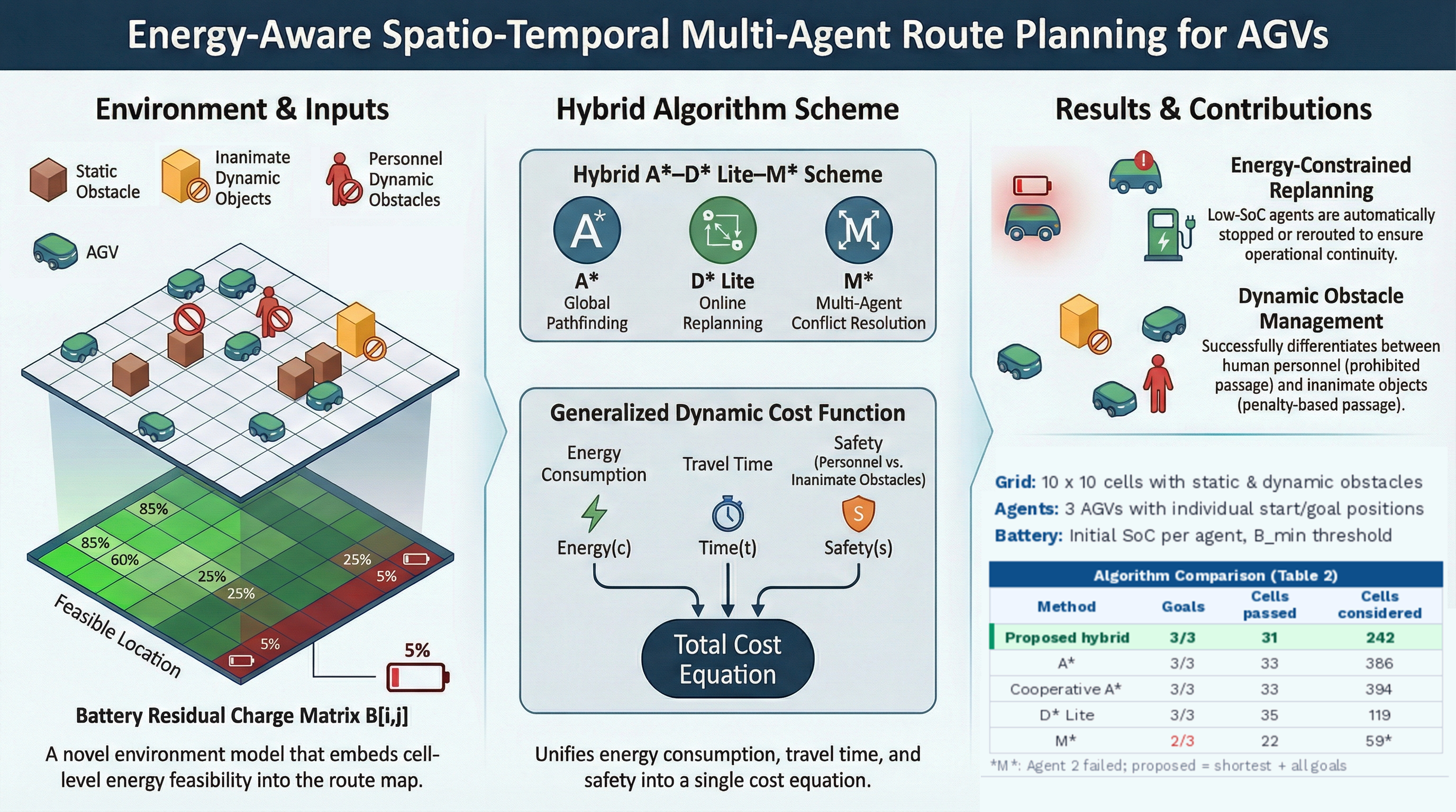
This article addresses the problem of finding the shortest route for Automated Guided Vehicles (AGVs) in a production environment with constrained battery state-of-charge (SoC) and time-dependent operating conditions. The route map is divided into a uniform grid containing stationary obstacles and two types of dynamic obstacles: human, for which AGV transportation is prohibited, and inanimate (moving objects), which impose a penalty function. A key contribution of the proposed methodology is the introduction of a battery residual charge matrix, which embeds cell-level energy feasibility into the environment representation by determining minimum admissible SoC constraints and accounting for transition-dependent energy costs. This matrix directly restricts the set of traversable cells under low-energy conditions. The proposed approach is based on the A* and D* Lite algorithms, providing shortest-path construction that explicitly integrates battery SoC into the spatio-temporal cost function. To avoid collisions in a multi-agent environment during routing, a simplified hybrid scheme with M* elements performs local coordination and adaptive trajectory replanning. The effectiveness of the proposed methodology was assessed using travel time, temporal complexity, and spatial complexity metrics. Simulation results on a 10×10 grid showed that agents with sufficient battery completed routes of 8 and 11 cells with travel times of 7.2 to 10.7 conventional units. A critically low-energy agent was initially unable to move, but after adjusting the minimum SoC constraint, all agents completed their routes with travel times up to 11.4 conventional units, demonstrating the direct impact of energy constraints on system performance.
Keywords:
spatio-temporal path planning
; multi-agent systems
; battery state-of-charge
; energy constraints
; Automated Guided Vehicle
1. Introduction
Automated Guided Vehicles (AGVs) are essential components of modern industrial logistics, enabling flexible and efficient material transport in manufacturing and warehouse environments. Effective AGV route planning must address multiple challenges simultaneously: managing energy constraints, avoiding static infrastructure, responding to dynamic obstacles (including personnel), and coordinating multiple agents. While numerous path-planning methods exist, few approaches account for all these factors, particularly the integration of real-time battery state into routing decisions. This gap motivates the development of a comprehensive methodology that balances route optimality, safety, and energy efficiency.
This research proposes a route-planning methodology for a multi-agent AGV system subject to energy and time constraints, accounting for static and dynamic obstacles of various types. The methodology aims to ensure that each agent reliably reaches the target while minimizing route length and travel time and enhancing system robustness by incorporating residual battery charge as a planning constraint through adaptive, cell-level energy thresholds (i.e., a battery charge matrix as an additional component of the environment state). It combines A*, D* Lite, and M* planning components, enabling local optimization and adaptive real-time trajectory replanning. The scientific novelty lies in introducing a dynamic spatio-temporal travel-cost function in which the current battery state-of-charge (SoC) explicitly constrains feasible routes and drives adaptive replanning in multi-agent settings. The effectiveness of the methodology is evaluated based on route execution time, collision count, and total energy expenditure.
The remainder of the paper is structured as follows. Section 2 reviews related work on AGV path planning. Section 3 introduces the mathematical foundation of the proposed hybrid A*–D* Lite–M* methodology for multi-agent AGV route optimization under battery-charge constraints, static and dynamic obstacles, and time limitations. Section 4 describes the experimental setup, including grid configuration, obstacle matrices, and simulation parameters. Section 5 presents numerical results based on simulated AGV trajectories in a grid environment with personnel and movable-object interference. Section 6 compares the effectiveness of the proposed approach with baseline A*, D*, and M*-based approaches in terms of route optimality, computation time, and adaptability to dynamic environmental changes. Our conclusions are presented in Section 7, where the obtained results are summarized, and proposals for future research are outlined.
2. Related Works
Publications [1,2,3,4] are review articles. In [1], a review on route planning approaches in multi-agent systems is presented, including the classification of A*-based methods, heuristic approaches, biologically inspired techniques, and artificial intelligence (AI)-based algorithms. It is shown that many existing approaches do not account for battery constraints or time-varying moving obstacles. Article [2] focuses on the route planning and control of mobile robots, including AGVs and Autonomous Mobile Robots (AMRs) in logistics environments (warehouses and intralogistics) based on a control model combined with layered planning (task scheduling and motion planning) while considering constraints in complex intralogistics settings. In [3], a review of modern methods of path planning in dynamic environments for various robotic systems is conducted. Sensor modalities, obstacle types, planning strategies (avoid, plan, replan), and key challenges (adaptation time, inter-agent communication) are analyzed. A classification of planning approaches is provided, and weaknesses are identified, particularly in multi-step planning for dynamic agents. In [4], the authors present a comprehensive survey on path planning methods for dynamic environments. They categorize existing approaches into constraint-based, dynamic, and multi-agent and highlight open research gaps. Particular attention is drawn to the necessity of integrating battery limitations, dynamic obstacles, and inter-agent coordination.
In [5], the authors enhanced the A* algorithm in combination with the Dynamic Window Approach (DWA) for AGVs operating in factory environments with both dynamic and static obstacles. The method dynamically adjusts the heuristic weight in A* based on obstacle density and integrates it with DWA for local adaptation. As a result, the planning time is reduced, and the generated route is smoother than that produced by classical A*. Research [6] proposes a path planning system for multi-agent manufacturing environments based on an improved A* algorithm. The results show that the approach enhances agent coordination and reduces conflicts in shared spaces with cooperating AGVs. In [7], a dynamic path planning method is proposed for an AGV that follows a moving target using integrated sensory and visual information. The results demonstrate that the AGV successfully tracks a moving target in changing environments using the proposed method.
In [8], D* Lite was used in a conflict-based search for multi-task routing. This enabled the integration of dynamic replanning with the detection of potential conflicts among agents. A comparison with the standard approach shows a reduction in the number of disputes and an improvement in planning success under conditions of obstacles. An algorithm for planning a route for an AGV operating in a dynamic environment, based on A* and DWA, is proposed in [9]. A feature of this study is the inclusion of route adaptation to dynamic obstacles, accounting for speed and safety constraints. Experimental results show that the proposed hybrid approach exhibits better adaptability and shorter paths than the standalone A* and DWA algorithms. The authors of [10] developed a hybrid algorithm that utilizes kinematic-constraint A* with DWA for an AGV in a dynamic environment. The proposed algorithm reduces the path length by 3.6% and the local planning time by 50% compared with traditional methods. In [11], A* under AGV kinematic constraints was combined with local DWA planning in dynamic environments. As a result, the path generated by the global plan became smoother in terms of the number of turns and time compared to that of classical A*. In [12], a multi-criteria path planning algorithm was proposed, combining global Ant Colony Optimization (ACO) search to reduce the path cost and local optimization through a modified DWA. In simulations, the algorithm exhibited significant reductions in path length and the number of turns compared with the baseline. In [13], the authors improved A* with adaptive heuristics and a combination with DWA analysis in environments with different types of obstacles. That is, adaptive heuristics were applied with a search approach to increase efficiency and reduce redundant nodes. The results demonstrate an increase in planning efficiency, achieved by reducing the number of nodes and search time compared to basic A*.
In [14], an improved version of D* Lite for handling moving objects in dynamic settings is applied to an underwater vehicle for multi-goal planning and collision avoidance in an unknown dynamic environment. The results show that the modified D* Lite plans efficient routes under non-static conditions and, compared to the basic versions, achieves a higher success rate. Work [15] is dedicated to a hybrid framework that combines D* Lite as a global planner and Multi-Agent Reinforcement Learning (MARL) for local decisions in an environment with dynamic obstacles and changing states using a "switching" mechanism between the global planner and the local learning agent while maintaining operability when the environment changes. As a result, multi-agent planning success improves, the number of conflicts decreases, and path efficiency increases relative to a purely centralized approach. In [16], the authors propose a path planning scheme for AGV trajectory control in terminals with both static and dynamic obstacles. It is shown that the proposed scheme effectively bypasses obstacles and increases trajectory stability. Paper [17] presents a multi-agent system with centralized decision-making that uses D* Lite to account for autonomous behavior and coordination in the presence of conflicts and interactions between agents. It is shown that the scheme enables the coordination of agents’ routes and replanning in a changing environment. In [18], the authors presented an improved potential field method for multiple AGVs in a dynamic port environment that accounts for the minimum safe distance between AGVs and the dynamic repulsive potential. The algorithm adapts to environmental changes in real time, reducing the probability of collisions.
Methods using AI are presented in publications [19,20,21,22,23,24,25]. In [19], an optimized shortest-path model for AGVs based on a support vector machine (SVM) was developed, resulting in increased planning efficiency under complex production conditions. In [20], a review of path-planning approaches for multiple mobile robots was conducted, covering classical, heuristic, and AI-based methods. The authors emphasized the trend toward decentralized planning in multi-robot systems and identified key challenges, including real-time operation, resource constraints, and inter-robot coordination. In [21], a dynamic multi-criteria path-planning model based on multi-agent deep reinforcement learning (MADRL) was proposed. It has been shown that agents can reach their targets while simultaneously optimizing multiple criteria, such as time, distance, and the number of turns, in complex environments. In [22], a hybrid AGV path-optimization algorithm was introduced, integrating the evolutionary Grey Wolf Optimizer (GWO) algorithm with local partially matched crossover (PMX) mutation to improve route smoothness and length. Experiments confirmed that the evolved routes are smoother and shorter than those of classical heuristic approaches. The novelty of the approach in [23] lies in combining a learning-based method (a K-L network enhanced with a genetic algorithm) with global planning to achieve smoother navigation paths. The results demonstrate effective avoidance of dynamic obstacles and improved coordination among multiple AGVs. In [24], deep reinforcement learning methods—specifically Deep Deterministic Policy Gradient (DDPG) and Multi-Agent Deep Deterministic Policy Gradient (MADDPG)—were applied for cooperative AGV navigation in dynamic environments with obstacle avoidance. The novelty of the method lies in centralized training with decentralized execution and optimized experience buffers. The study shows that agents successfully coordinate and avoid collisions, thereby reducing travel time and conflicts. Paper [25] proposes an intelligent motion-control system for a wheeled mobile robotic platform that integrates navigation, fuzzy logic, and advanced sensor-data processing to ensure adaptive behavior in dynamic environments. The novelty lies in the development of a rule-based fuzzy controller and a remote software implementation, with simulation results demonstrating effective platform motion under varying sensor conditions.
Publications [26,27,28,29] consider the remaining SoC. In [26], a priority-based scheduling approach for AGVs using the ACO algorithm for collision avoidance is proposed, with the AGVs’ battery level determining the collision avoidance priority. Experimental results confirm that battery-based prioritization reduces conflicts and improves AGV traffic efficiency in a factory. The authors of [27] consider the problem of real-time dispatching of an AGV fleet under battery constraints. The proposed solution based on deep reinforcement learning demonstrated improvements in both battery-utilization efficiency and overall system performance. The authors of [28] developed a task-scheduling method for AGVs under battery constraints that combines task redistribution, charging management via a Gurobi/LP module, and optimization using a battery-threshold policy. The results demonstrate industry-applicable solutions that minimize delays and traffic-related costs. In [29], optimization of AGV routing and loading schedules in a container terminal, accounting for load-flow dynamics, is considered. The novelty of the approach lies in a dual-threshold charging strategy adapted to load-flow conditions, integrated with routing and scheduling. The results are verified through simulations, and it is validated that the flexible charging strategy increases AGV availability and reduces downtime.
Based on the conducted literature review, most approaches for AGV route planning can be grouped into the following categories:
- 1.
- Classical heuristic and graph-search methods, including A*, Dijkstra, D*, D* Lite, Theta*, Lifelong Planning A*, etc. They guarantee the existence of an optimal or approximate route. However, these methods suffer from high computational complexity when scaled to large or dynamic environments and generally do not account for the remaining AGV battery charge.
- 2.
- Local optimization methods, including the DWA, Artificial Potential Field (APF), Velocity Obstacle (VO), and their improved variants. They may implicitly account for energy consumption through constraints on maximum speed or acceleration.
- 3.
- Evolutionary and swarm-intelligence methods, such as Genetic Algorithms (GA), ACO, Particle Swarm Optimization (PSO), GWO, etc. These approaches perform well for multi-criteria tasks but often require many iterations and are unstable in dynamic environments. Therefore, they are effective for real-time tasks but are prone to local minima and do not guarantee a global optimum. They can incorporate energy as an optimization criterion, but in a simplified manner, without dynamic discharge modeling or constraints on returning to the charging station.
- 4.
- Machine Learning and Reinforcement Learning methods, such as Deep Q-Learning, DDPG, Proximal Policy Optimization (PPO), MADDPG, and Graph Neural Networks (GNNs), for multi-agent planning. These methods enable AGVs to adapt their behavior to environmental changes but require large amounts of training data and substantial computational resources. They can incorporate SoC into the state space. However, literature analysis shows that these methods typically model only a minimum SoC constraint after which the AGV must return to charging and do not address battery degradation or inter-cell charge variation.
- 5.
- Hybrid methods integrate global planners (e.g., A*, D*) with local obstacle-avoidance techniques (e.g., DWA, APF) or combine heuristic methods with reinforcement learning or evolutionary algorithms. They strive to balance speed, adaptability, and accuracy, yet most studies do not jointly consider energy constraints, time efficiency, and the presence of live dynamic obstacles. In such methods, battery considerations are typically limited to pre-planned charging-point routing or are completely ignored in agent-coordination scenarios.
Thus, key research gaps include the inadequate integration of energy management, adaptive dynamic obstacle avoidance, and stable route execution in multi-agent environments.
3. Materials and Methods
In this paper, we propose a hybrid methodology for determining the shortest routes between destinations for AGVs that accounts for limited resources, including:
- the number of grid cells into which the map of the premises, along with the route that the AGV must travel, is divided;
- stationary obstacles where AGV transportation is prohibited;
- dynamic obstacles, which are categorized into human (personnel) and inanimate, such as boxes, pallets, etc., that accidentally appear on the AGV’s path and can be rearranged;
- the remaining charge of the AGV’s battery;
- the time spent traveling through the cells.
In the proposed methodology, the generalized dynamic travel-cost function is defined as (1):
where:
| — dynamic transit cost of moving from node u to v at time step t; | |
| — estimated energy consumption for the transition from u to v; | |
| — traversal time for the transition from u to v, including base time, turns, and delays due to dynamic obstacles; | |
| — static obstacle indicator at target cell v; | |
| — inanimate dynamic obstacle indicator at cell v at time t; | |
| — human dynamic obstacle indicator at cell v at time t; | |
| — weighting factors; | |
| — sufficiently large penalty constant (e.g.,). |
The coefficient determines the penalty associated with static obstacles. At very large values, the cell becomes inadmissible (analogous to a hard constraint, as used in this work), and at significant values, cells near obstacles can be used, accounting for risk or additional costs. The relative value of compared to and determines the system priorities. For example, if , then safety with respect to static objects dominates, and if , then obstacles are accounted for as an additional cost factor alongside energy consumption and time.
Within this framework, A* constructs an initial minimum-cost route, D* Lite updates it online as the environment/battery SoC changes, and M* resolves local multi-agent conflicts when paths interact. Therefore, we introduce these routing algorithms next and then show how they are combined in the hybrid scheme.
3.1. Algorithms for Finding the Shortest AGV Route
3.1.1. A* Algorithm
A* is a starting algorithm for local search for the shortest AGV route on a graph with edge weights. Its main advantage lies in combining a breadth-first search with a greedy search. The basic principle of A* is to compute the cost function (2) for each vertex u:
where:
| — estimated total path cost through node u; | |
| — accumulated path cost from the start node to node u; | |
| — heuristic estimate of the cost from node u to the target node. |
The following steps summarize the standard A* search loop used to expand candidate nodes and update path costs1:
- Place the starting vertex in the open list. While the open list is not empty, select the vertex u with the smallest . If u is the target vertex, terminate the search and move it to the closed list.
- For each neighbor v of node u, we calculate the accumulated cost to reach the neighbor node v via node u as (3):
- Update the priority of affected nodes in the open list and continue by expanding the node with the smallest evaluation function (2).
The A* algorithm guarantees finding the optimal path if its heuristic function is admissible. The time complexity depends on the accuracy of the heuristic .
3.1.2. D* and D* Lite Algorithms
The D* algorithm enables dynamic updates to edge weights or node accessibility during the AGV motion. The accumulated cost for each node follows the same relaxation rule as in (3). If the graph changes, only affected nodes are updated. D* Lite works backward from the target to the start. It uses the g-value and rhs-value (one-step lookahead value of node u to determine node consistency): if , the node is consistent; otherwise, it is inconsistent and requires processing. For D* Lite, the -value is defined as (4):
If a node v has not yet been considered, i.e., is not on the closed list, then a better path has been found; add v to the open list. The key-function used for the node u in the D* Lite priority queue is defined in detail in Section 3.3, equations (16), (17), (18). The main steps are:
- 1.
- Initialization: , . Add goal to the priority queue.
- 2.
- While start is inconsistent or start-key < queue-key, remove nodes with a minimum key; update and neighbors, maintaining consistency.
- 3.
- During agent movement: if new obstacles appear or weights change, update only for affected nodes; recalculate path only for inconsistent nodes.
D* Lite performs fewer computations than D* because it does not need to recalculate the entire graph. It enables optimal, adaptive replanning in dynamic environments for AGVs moving across a map with unpredictable obstacles.
3.1.3. M* Algorithm
The M* algorithm is an extension of A* for problems with multiple agents moving simultaneously in a shared environment by searching the joint state space only when conflicts occur. For K agents, a joint state is where is the current cell of agent i. Conflicts include vertex collisions (same cell, same time) and edge collisions (agents swapping cells).
The main steps are:
- 1.
- Compute individual shortest paths using .
- 2.
- Detect conflicts along these paths.
- 3.
- If a conflict is found, temporarily couple only the conflicting agents and replan locally; otherwise, execute the next step.
- 4.
- Repeat until all agents reach their goals.
M* performs joint replanning only where needed, reducing the cost of full K-dimensional search.
3.2. Setting Constraints to Find the Shortest AGV Route
3.2.1. Grid Discretization
Figure 1 shows the route map window during the movement of the AGV in the "Navitrol Monitor" environment. The brown color indicates stationary obstacles included in the AGV route map (walls, cabinets, and fixed workstations). The green color indicates what the AGV detects during motion using 2D LiDAR. Since this AGV is equipped with only a single front-facing LiDAR, areas behind it remain temporarily invisible. The green circles denote the points between which the AGV moves while performing its tasks; their combination forms a trajectory that corresponds to the AGV’s predefined goals.
The map of the room where the AGV and personnel operate is divided into a grid of uniformly sized squares, with dimensions in the horizontal and vertical directions, respectively.
The grid is represented as a graph , where the vertices V correspond to the cells of the grid, and the edges represent the connections between the four adjacent neighboring cells.
Each node corresponds to a unique grid cell at position , where i and j denote the row and column indices, respectively. When defining environment matrices (e.g., ), the indices refer to the grid coordinates of the corresponding node u.
3.2.2. Stationary Obstacles
If in the matrix of static obstacles , this indicates a stationary obstacle where AGV movement is prohibited (marked on the map with brown lines or dots occupying the corresponding cell). Such obstacles include walls, fixed tables, workstations, fenced areas around various robotic setups, and similar structures. Conversely, represents a free cell where AGV movement is allowed (no brown lines or dots are present). This matrix is static, uniform, and constant across all AGVs. Changes occur only if the room layout is modified or new stationary obstacles are introduced. Next, all constraints must be defined, including spatial limits, masking areas, and proximity restrictions.
3.2.3. The Remaining Charge of the AGV Battery
In the proposed approach, the AGV battery SoC directly affects the route planning process through two mechanisms: the availability of cells in the workspace and the energy component of the travel cost function.
The first mechanism is implemented via a cell-availability mask, , which characterizes the minimum fraction of charge required to pass through a particular cell. The constraint is the battery charge mask , given as an matrix that determines whether the agent (AGV) can be in this cell according to energy constraints. if the cell is inaccessible to the agent (mainly due to stationary obstacles). If (for the maximum battery charge) or a specific value: for the remaining SoC, then the cell is accessible. At the same time, energy costs can be taken into account (5):
where:
| — set of indices for which the matrix B has defined values greater than or equal to ; | |
| — minimum threshold value to include the entry in ( is the minimum technologically permissible discharge threshold for AGV Formica 1, below which the cell is inaccessible). |
The second mechanism is based on the dynamic function , in which the component represents the energy cost of transitioning between cells. This value accounts for key AGV motion characteristics, including acceleration, braking, required stops, turns, and potential local obstacles that induce additional energy losses. The weight of this component is modulated by the coefficient , which determines the relative importance of energy efficiency compared to other routing factors. A higher value of encourages the algorithm to favor transitions with lower energy consumption. Consequently, even without an explicit dependence on the battery’s SoC, the energy cost indirectly reflects the AGV’s limited energy resources, leading the AGV to naturally select more energy-efficient trajectories at lower SoC levels.
3.2.4. Dynamic Obstacles
Two types of dynamic obstacles are considered: human obstacles (personnel), which prohibit AGV passage through the occupied cell, and inanimate obstacles (e.g., pallets, boxes, moving objects), which do not block the cell permanently but increase the local traversal cost. We introduce the time-dependent occupancy matrices and , where if a person occupies node u at time t, and if an inanimate obstacle occupies node u at time t. The overall dynamic occupancy is (6):
A node u is considered traversable at time t if it is not a static obstacle, not occupied by a person, and satisfies the battery-threshold constraint. The corresponding accessibility mask is defined as (7):
where is the indicator function.
In general, movement is allowed only between four horizontally/vertically adjacent cells (no diagonal moves). The 4-neighborhood of a cell , constrained to the grid, is defined as (8):
For example, in cell , the 4-neighborhood includes the cells , , , and . For modeling purposes, we assume that a dynamic obstacle moves by one cell per time step in one of the four directions:
where: — obstacle position (cell index) at time step t; — move to a neighboring cell in one of the four directions.
For a move into a free cell, we set the base traversal cost to 1. Inanimate obstacles impose an additive penalty, whereas human obstacles make the cell inaccessible. The inanimate-obstacle penalty component is represented by (10):
where:
| — traversal cost of moving from cell u to cell v at time t; | |
| — penalty coefficient for inanimate dynamic obstacles; | |
| — occupancy indicator of inanimate obstacles at cell v at time t. |
Equation (10) is a special case of the generalized dynamic cost function (1) under simplified scheduling conditions. It describes a local model of the cost of passing a cell, accounting only for the basic step and the penalty associated with a non-living dynamic obstacle. It is applicable to basic A*-search or to the analysis of dynamic coordination between agents in isolation.
3.2.5. The Time Spent Traveling Through Cells
Because the generalized cost function in (1) explicitly includes the time component , it is important to define the traversal-time model used in simulations. The basic time to pass through a single free cell, with no obstacles and no penalties, defined as (11), is computed from the cell geometry and the average AGV speed.
where: L — length of the cell side, and — average linear speed of the AGV while moving in the free zone.
However, in real traffic conditions, there are additional time delays with which the total traversal time from u to v can be estimated by the expression (12):
where: — additional time for turning (depends on the angle of change of direction of movement); — additional delay due to the presence of dynamic obstacles.
The delay associated with a turn is described as (13):
where: — coefficient that takes into account the kinematic features of the AGV; — angle of change of direction (in radians).
In the presence of dynamic obstacles in neighboring cells, the AGV’s speed decreases, resulting in an increased transition duration (14):
where: — coefficient representing the influence of obstacles on AGV movement; — minimum distance to the nearest dynamic obstacle.
3.3. Proposed Methodology for Finding the Shortest AGV Route
Start the search for the shortest path from the starting cell to the goal, accounting for movement costs and the A* heuristic. Let:
| s | — the starting node, |
| q | — the goal node, |
| — accumulated cost to reach node u from the start node, | |
| — heuristic estimate from s to the goal u (e.g., Manhattan distance, ), | |
| — the evaluation function for the priority queue, | |
| — cost of moving from node to neighbor from u to v. |
Recursive update when moving from a node to a neighbor is carried out according to the expression if then , as in (15):
where: E — set of graph edges; — edge from node u to node v in the graph.
D* Lite is used for local adaptivity, i.e., it updates the current path when dynamic obstacles change the map (e.g., when people move). In the simplest implementation, a naïve strategy would rerun A* from scratch after each change; however, this is computationally expensive. In its classical form, D* Lite relies on the two functions: , defined in (4), and . To calculate the first component of the priority key for node u in D* Lite, combining its current best-known cost, one-step preview score, heuristic distance from the origin, and map change modifier, we use the formula (16):
where: — incremental modifier used to update keys when the map changes; - heuristic distance from the start position to node u (note that D* Lite searches backward from the goal)
To calculate the second component of the priority key for node u in D* Lite, taking the minimum of its current best-known value and the one-step preview estimate, we use the formula (17):
This formula defines the priority key of node u in D* Lite as a tuple , which is used to order nodes in the priority queue based on their estimated cost and heuristic (18):
The basic recalculation cycle is given by (19):
where: — the smallest key in the priority queue.
We take the node u with the minimum . If , where is the current best-known cost to reach node u and is the one-step lookahead value estimating the cost to reach u, then we make the node consistent: ; otherwise, if , we set and discard the previous u.
3.4. Multi-Agent Path Planning with Dynamic Obstacles
To ensure collision-free motion, we prohibit (i) vertex conflicts (two agents occupying the same cell at the same time) and (ii) edge conflicts (two agents swapping cells between consecutive time steps). In addition, movements must respect the static-obstacle mask, the human-obstacle constraint, and the battery-threshold constraint.
For a given agent at cell u and time step t, we restrict candidate moves to feasible neighbors 2. The local one-step update can then be written in the standard shortest-path form (20):
The transition cost is based on the same interpretation as in the dynamic-cost model (base cost plus an inanimate-obstacle penalty, and for infeasible cells). A compact definition used in simulations is (21):
where:
| — transition cost from u to v at time t; | |
| — feasibility indicator of cell v, see (7); | |
| — inanimate-obstacle indicator at cell v at time t; | |
| — penalty coefficient for inanimate obstacles (in this research, we use ). |
Equation (21) generalizes (10) by retaining the same base value of 1, adding a validity check via the accessibility indicator (7), and introducing an infinite cost for infeasible cells. That is, if the cell is admissible (), equation (21) reduces to (10), and if then corresponds to a hard restriction on passing through the cell.
The minimum technically permissible battery discharge is typically 20% for AGV Formica 1. The computational complexity of full M* considering K agents is , where K — number of agents; branches — average number of possible moves per agent. The simplified version reduces complexity by using a function similar to A*. The cost accumulation and node evaluation follow the same relaxation and priority rules defined in equations (3) and (2), respectively. The next step selection function is (22):
where: — best neighbor according to f-value. The total availability of the cell for the agent (23):
where — set of cells temporarily occupied by other agents at time t. Remaining path length after partial path execution (24):
where — remaining steps in partially constructed path. SoC constraint update (25):
where: — minimal battery required for the remaining path; — allowed minimal battery; — coefficient per remaining step. The coefficient 0.01 corresponds to an estimated 1% battery consumption per cell transition, derived empirically from the AGV Formica 1 specifications. Conflict detection with neighboring agents (26):
where:
| — set of agents in vertex or edge conflict; | |
| — current agent position; | |
| — other agent position; | |
| — adjacency condition. |
After all agents execute their moves, the position vector is updated to the new positions and the simulation clock advances by one discrete step. Boolean goal reached indicator (28):
Execution results summary (29):
where — final record of agent i, including the path, visited cells, order, reached flag, and stop reason. The total number of synchronous simulation steps is defined as , with discrete time .
The formulas described above follow the classical structure and operational rules of the A*, D* Lite, and M* algorithms; however, the key novelty lies in the author’s modifications, which include the integration of two types of dynamic obstacles (people and moving objects), as well as taking into account the remaining SoC of each AGV and the restrictions on the minimum allowable energy level, along with adaptive route replanning that considers these factors. Thus, the proposed changes will ensure that all agents reach the target point while optimally utilizing energy resources in a multifactor dynamic environment.
3.5. The Submodule Architecture
The main route planner receives the following: the AGV’s initial and target coordinates, matrices of static and dynamic obstacles, and a matrix of residual battery charges. The A* submodule is used to quickly build a route in small areas of the map with a relatively small number of variable obstacles. The D* Lite submodule is used to adapt the route in dynamic environments when moving objects appear, or battery data is updated. The M* submodule is used to coordinate multiple AGVs when routes intersect or conflicts must be avoided.
Each submodule returns a route, predicted time, and charge parameters. The main planner compares alternatives and selects a path that minimizes the total cost function, ensures the person’s safety (with a complete stop of the AGV) and safety from other dynamic obstacles, and guarantees sufficient battery balance. At each step of the AGV’s motion, the main planner checks the battery state and dynamic obstacles. In case of a conflict, the route is reconstructed by calling D* Lite and M* again.
4. Experimental Setup
Let us set the constraints for the traffic map shown in Figure 1, namely, the part of the 10 by 10 grid that covers points 23, 25, 26, and 30, over which the AGV traveled. Then the stationary constraint matrix will have the form (30):
In the same way, matrices are created for other parts of the grid. The map is partitioned so that, if all AGVs are in a single part, the entire map need not be recalculated. In this case, it is advisable to recalculate the shortest route only within this part of the map.
A key contribution is the introduction of the battery residual charge matrix of each AGV, which encodes cell-level energy feasibility and defines minimum admissible SoC constraints for route planning. In this matrix, Nones are at the locations of stationary obstacles (1 in the stationary-obstacle matrix), since it makes no sense to compute the battery-reserve charge, as AGV passage is prohibited there. In other cases, values are assigned using various methods, with neural networks and hybrid methods being the most effective. The authors in previous publications [30,31,32] proposed such methods of short- and medium-term forecasting. The residual charge calculated for each cell is normalized to the absolute maximum value in . Residual charge values are normalized to [0,1] using the maximum capacity of each AGV battery, reflecting both battery characteristics and degradation. Then it will describe the discharge more accurately, accounting for both the battery’s characteristics and condition and the operating modes of a particular AGV.
For example, three AGVs are running within the allowed cells. The agents start from cells , first, second, and third, respectively, and go to cells . For example, for the first AGV, the discharge matrix of the accumulator battery, assuming a full charge, will have the form (31):
For the second AGVs, the discharge matrix of the accumulator battery, assuming a full charge, will have the form (32):
For the third AGVs, the battery discharge matrix, taking into account the full charge, will have the form (33):
Dynamic obstacles are categorized as human (personnel) and inanimate (moving objects), with human obstacles prohibiting AGV passage and inanimate obstacles imposing a penalty function. Let two employees move cyclically along the route. The first starts at cell , where cell numbering begins at zero and proceeds along the following sequence of cells: . The second employee starts in cell and moves cyclically through the cells . Inanimate dynamic obstacles move along routes through the cells and , respectively. To determine a person’s position in space within the map grid, the methods developed by the authors [33] can be used.
Empirically determined parameters:
- the coefficient of influence of the turn, which takes into account the delay of the AGV when changing direction;
- the coefficient of influence of dynamic obstacles, which estimates the additional time due to the proximity of moving objects;
- the basic time of passage of a free cell, determined based on the average speed of the AGV.
Conditionally accepted parameters:
- cell side length, chosen for the unification of calculations;
- the minimum allowable battery charge level, taken as a safety threshold;
- penalties for passing through cells with moving objects, determined as conditional values for modeling the difficulty of passage.
Each AGV locally evaluates the dynamic cell cost, including residual SoC, static obstacles, and penalties from dynamic obstacles, enabling adaptive local route planning. The deep neural network–based battery remaining prediction module is executed locally on each agent, and the resulting neural network weights can be transmitted to a central server for aggregation. Each AGV can then update its transit-time matrix, assess the risks posed by dynamic obstacles, and construct optimal routes based on updated energy consumption and environmental forecasts. This approach reduces traffic between the AGV and the server and enhances data confidentiality. It also enables dynamic, real-time route adaptation that accounts for energy constraints and environmental changes.
5. Results
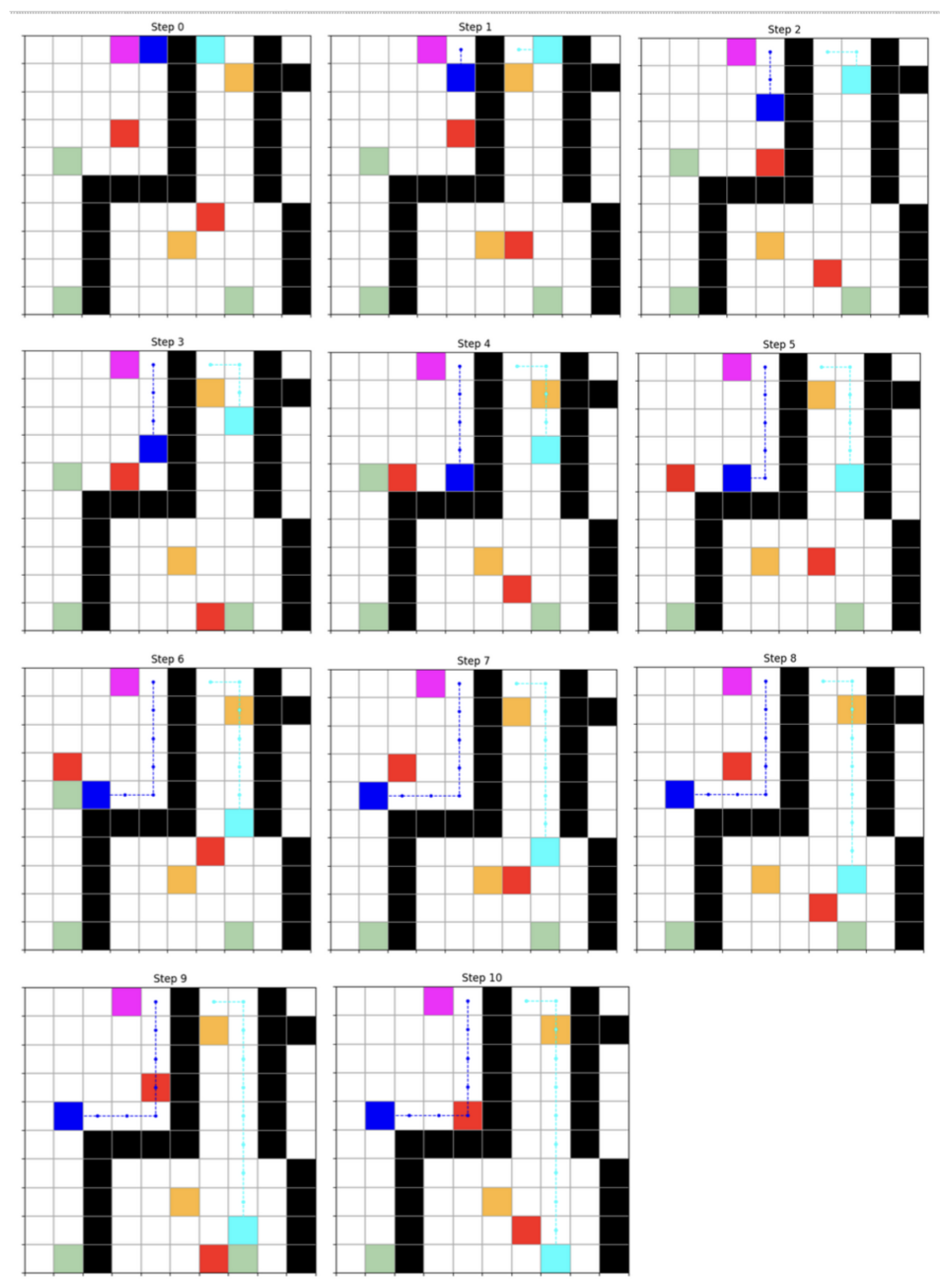
The simulation was executed using the parameters defined in the experimental setup: cell side length of 1.0 (conventional length unit), average AGV speed of 1.0 (conventional length unit per time unit), turning-angle influence coefficient of 0.2, and dynamic-obstacle influence coefficient of 0.5. The methodology’s effectiveness is evaluated using three metrics: travel time, spatial complexity, and temporal complexity. The resulting paths are depicted in Figure A1.
In Figure A1, black indicates stationary obstacles where AGV passage is prohibited. These cells are assigned a value of 1 in the static-obstacle matrix and are marked as None in the predicted residual battery-charge matrices. Purple, blue, and turquoise represent three AGVs, while green denotes their target points. Yellow and red indicate dynamic obstacles: red denotes people; if an AGV and a person occupy the same cell, passage is prohibited, forcing the AGV to wait until the cell is released. Yellow represents non-visible dynamic obstacles that impose a penalty for passing through the cell. If the penalty value is high (close to 5), the path is planned to circumvent the obstacle; if it is low, the AGV may traverse the cell and wait if it is occupied upon approach.
The methodology prevents AGVs from occupying the same cell simultaneously, applying local conflict resolution as in M* to replan trajectories when conflicts occur. If an AGV encounters another AGV or a dynamic obstacle, it waits one step before releasing the cell. If the cell remains occupied, a new "detour route" is constructed. As observed, Agent 3 did not move because, after attempting to build a route to the target cell, it became evident that the remaining SoC would be insufficient (Table 8).
Additional simulations with varying numbers of AGVs confirmed the effectiveness of the proposed approach in maintaining shortest paths while respecting energy and obstacle constraints. A comparison of the results obtained with the proposed methodology against other methods for finding the shortest route under constraints is presented in Table 9.
Analyzing the results presented in Table 9, it is evident that different route-planning methods differ significantly in efficiency and reliability in achieving their goals. Given that the primary requirement is for each agent to follow the shortest route while ensuring sufficient remaining SoC and accounting for obstacles, the following conclusions can be drawn:
The A* and Cooperative A* methods guarantee reliable goal achievement for all agents, albeit at the cost of evaluating a significantly larger number of cells during route planning. The D* Lite method demonstrates a balance between efficiency and computational cost, enabling agents to reach their goals while considering a moderate number of cells and adapting routes in dynamic environments. However, the resulting routes are not highly optimized. The M* method proved to be the most economical in terms of the number of evaluated cells, but it exhibits instability; in particular, Agent 2 was unable to reach its goal, making this method risky for guaranteed route planning. The proposed methodology ensures goal achievement along the shortest routes, although the number of evaluated cells is slightly higher than that of the most economical methods. Nevertheless, it is the only approach that guarantees the shortest route for all agents, accounts for both dynamic and static obstacles, and respects the limit on the remaining SoC. Furthermore, the maximum number of evaluated cells is moderate compared with that of all methods. Therefore, the proposed methodology represents a compromise solution between efficiency, reliability, and computational cost.
6. Discussion
The results demonstrate the effectiveness of the proposed multi-agent AGV planning methodology, which simultaneously considers residual SoC, static and dynamic obstacles, and time costs to traverse the route. For Agent 1, a stable route was built; it completed the task without stopping, and the remaining SoC after route completion was (or due to expectations). This indicates the efficient use of energy resources for a short route and the absence of critical situations. For Agent 2, the longest route (11 cells) was found with a passage time of 10.70 conventional units and a remaining charge of and due to expectations. The agent completed the task in full, without reaching a critical energy level. This confirms that even with a longer trajectory, the algorithm supports stable operation of the energy management system. For Agent 3, the initial simulation recorded a stop due to reaching the minimum allowable battery charge (battery_low, remaining for the constructed route). As a result, the route consisted of a single cell, indicating that the energy limitation criterion operated correctly. After adapting the residual charge matrix (setting the minimum threshold to 0.2), the agent passed 12 cells in conventional units, completing the task without stopping. The remaining SoC was , i.e., above the minimum allowable level. This confirms that adjusting the energy parameters in the residual charge matrix directly affects the reachability of the target coordinates and the total task execution time. A comparison of the two simulation series showed that even a slight change in the minimum allowable charge level (from to ) significantly improves the functional reliability of the AGV system, allowing agent 3 to complete the route without an emergency stop.
The reported results are obtained under simplifying conditions that constrain the scope of the conclusions. In particular, the experiments assume a fixed fleet size (i.e., a predefined number of AGVs on the map) and a prescribed minimum battery-charge threshold that determines whether motion is permitted. The AGV base speed is treated as constant; therefore, effects such as load-dependent dynamics, acceleration limits, and speed-control policies are not explicitly modeled. In addition, the behavior of dynamic obstacles is represented through selected motion characteristics (e.g., speed and cyclic trajectories), which may not fully capture irregular human behavior or non-periodic disturbances typical of real production floors. Finally, the motion model is restricted to 4-connected grid transitions (up/down/left/right), excluding diagonal moves. While this simplifies conflict detection and replanning, it may overestimate path length relative to continuous-space navigation.
Future research will focus on extending the framework toward more realistic industrial conditions by (i) incorporating variable-speed and load-dependent energy models, (ii) supporting 8-connected and continuous-space motion primitives, (iii) improving prediction and uncertainty handling for human motion and non-cyclic dynamic obstacles, and (iv) validating the approach on larger maps and real AGV deployments with online sensing and communication constraints.
7. Conclusions
The results demonstrate the effectiveness of the proposed methodology for route planning in a multi-agent AGV system under energy and time constraints, accounting for static and two types of dynamic obstacles. In light of prior studies, the results confirm that incorporating dynamic battery charge estimation and adaptive thresholds significantly enhances route stability and system robustness. Earlier research on AGV coordination often focused on geometric optimization or obstacle avoidance. However, fewer studies have examined the energy–reliability trade-off in decentralized multi-agent control frameworks. From the perspective of the initial working hypothesis, the results validate that incorporating a dynamic energy constraint into the routing algorithm directly improves both the robustness and functional reliability of AGV fleets. The agents successfully balanced travel time and residual energy, indicating that the proposed model can be effectively applied to real-world industrial scenarios where energy efficiency and operational continuity are critical. Future research should focus on extending the proposed approach to: real-time adaptive control using predictive battery models (e.g., LSTM-based voltage forecasting); federated coordination among heterogeneous AGVs with varying energy consumption profiles; and integration of anomaly detection mechanisms to preemptively identify energy inefficiencies or sensor faults.
Author Contributions
Conceptualization, O.P., M.M.; methodology, O.P.; software, O.P. and M.M.; validation, O.P. and M.M.; formal analysis, O.P.; investigation, O.P. and M.M.; resources, O.P. and M.M.; data curation, O.P. and M.M.; writing—original draft preparation, O.P. and M.M.; writing—review and editing, O.P. and M.M.; visualization, O.P. and M.M.; supervision, O.P.; project administration, O.P.; funding acquisition, O.P. All authors have read and agreed to the published version of the manuscript.
Funding
Co-funded by the European Union HORIZON TMA MSCA Doctoral Networks / HORIZON-MSCA-2023-DN-01 / project TUAI / grant agreement N° 101168344. Views and opinions expressed are, however, those of the author(s) only and do not necessarily reflect those of the European Union or European Research Executive Agency. Neither the European Union nor the granting authority can be held responsible for them. Co-funded by the Statutory Research funds of the Department of Distributed Systems and Informatic Devices, Silesian University of Technology, Gliwice, Poland (Grants BK-244/RAu8/2025 02/110/BK_25/1036).
Data Availability Statement
All of the data presented in this study are available in publicly accessible repositories. Neural network prediction of battery discharge https://github.com/opavliuk1980/AGV_WP3, accessed on 03 November 2025. Human activity recognition https://github.com/opavliuk1980/HAR. Methodology for finding the shortest AGV route under limited resources https://github.com/opavliuk1980/Shortest-path-with-constraints. The proposed methodology https://github.com/opavliuk1980/methodology_MDPI.
Acknowledgments
During the preparation of this manuscript, the authors used Claude Opus 4.5 for the purposes of proofreading and Google NotebookLM for generating some visual elements for the graphical abstract. The authors have reviewed and edited the output and take full responsibility for the content of this publication.
Conflicts of Interest
The authors declare no conflicts of interest.
Appendix A
Figure A1.
The result of finding the shortest AGV path according to the proposed methodology.
References
- Banik, S.; Banik, S.C.; Mahmud, S.S. Path Planning Approaches in Multi-robot System: A Review. Engineering Reports 2025, 7. [Google Scholar] [CrossRef]
- Fragapane, G.; de Koster, R.; Sgarbossa, F.; Strandhagen, J.O. Planning and control of autonomous mobile robots for intralogistics: Literature review and research agenda. European Journal of Operational Research 2021, 294, 405–426. [Google Scholar] [CrossRef]
- AbuJabal, N.; Baziyad, M.; Fareh, R.; Brahmi, B.; Rabie, T.; Bettayeb, M. A Comprehensive Study of Recent Path-Planning Techniques in Dynamic Environments for Autonomous Robots. Sensors 2024, 24. [Google Scholar] [CrossRef] [PubMed]
- Jayalakshmi, K.P.; Nair, V.G.; Sathish, D. A Comprehensive Survey on Coverage Path Planning for Mobile Robots in Dynamic Environments. IEEE Access 2025, 13, 60158–60185. [Google Scholar] [CrossRef]
- Sang, W.; Yue, Y.; Zhai, K.; Lin, M. Research on AGV Path Planning Integrating an Improved A* Algorithm and DWA Algorithm. Applied Sciences 2024, 14. [Google Scholar] [CrossRef]
- Pratama, A.Y.; Ariyadi, M.R.; Tamara, M.N.; Purnomo, D.S.; Ramadhan, N.A.; Pramujati, B. Design of Path Planning System for Multi-Agent AGV Using A* Algorithm. In Proceedings of the 2023 International Electronics Symposium (IES), 2023; pp. 335–341. [Google Scholar] [CrossRef]
- Sun, M.; Lu, L.; Ni, H.; Wang, Y.; Gao, J. Research on dynamic path planning method of moving single target based on visual AGV. SN Applied Sciences 2022, 4, 86. [Google Scholar] [CrossRef]
- Jin, J.; Zhang, Y.; Zhou, Z.; Jin, M.; Yang, X.; Hu, F. Conflict-based search with D* lite algorithm for robot path planning in unknown dynamic environments. Computers and Electrical Engineering 2023, 105, 108473. [Google Scholar] [CrossRef]
- Wu, B.; Chi, X.; Zhao, C.; Zhang, W.; Lu, Y.; Jiang, D. Dynamic Path Planning for Forklift AGV Based on Smoothing A* and Improved DWA Hybrid Algorithm. Sensors 2022, 22. [Google Scholar] [CrossRef]
- Yin, X.; Cai, P.; Zhao, K.; Zhang, Y.; Zhou, Q.; Yao, D. Dynamic Path Planning of AGV Based on Kinematical Constraint A* Algorithm and Following DWA Fusion Algorithms. Sensors 2023, 23. [Google Scholar] [CrossRef]
- Gong, X.; Gao, Y.; Wang, F.; Zhu, D.; Zhao, W.; Wang, F.; Liu, Y. A Local Path Planning Algorithm for Robots Based on Improved DWA. Electronics 2024, 13. [Google Scholar] [CrossRef]
- Xiao, J.; Yu, X.; Sun, K.; Zhou, Z.; Zhou, G. Multiobjective path optimization of an indoor AGV based on an improved ACO-DWA. Mathematical Biosciences and Engineering 2022, 19, 12532–12557. [Google Scholar] [CrossRef] [PubMed]
- Sun, Y.; Yuan, Q.; Gao, Q.; Xu, L. A Multiple Environment Available Path Planning Based on an Improved A* Algorithm. International Journal of Computational Intelligence Systems 2024, 17, 172. [Google Scholar] [CrossRef]
- Zhu, X.; Yan, B.; Yue, Y. Path Planning and Collision Avoidance in Unknown Environments for USVs Based on an Improved D* Lite. Applied Sciences 2021, 11. [Google Scholar] [CrossRef]
- Liu, N.; Shen, S.; Kong, X.; Zhang, H.; Bräunl, T. Cooperative Hybrid Multi-Agent Pathfinding Based on Shared Exploration Maps. Journal of Intelligent & Robotic Systems 2025, 111, 97. [Google Scholar] [CrossRef]
- Feng, J.; Yang, Y.; Zhang, H.; Sun, S.; Xu, B. Path Planning and Trajectory Tracking for Autonomous Obstacle Avoidance in Automated Guided Vehicles at Automated Terminals. Axioms 2024, 13. [Google Scholar] [CrossRef]
- Ren, Z.; Rathinam, S.; Likhachev, M.; Choset, H. Multi-Objective Path-Based D* Lite. IEEE Robotics and Automation Letters 2022, 7, 3318–3325. [Google Scholar] [CrossRef]
- Chen, X.; Chen, C.; Wu, H.; Postolache, O.; Wu, Y. An improved artificial potential field method for multi-AGV path planning in ports. Intelligence & Robotics 2025, 5, 19–33. [Google Scholar] [CrossRef]
- Liu, R. Research on Optimization of the AGV Shortest-Path Model and Obstacle Avoidance Planning in Dynamic Environments. Mathematical Problems in Engineering 2022, 2022, 2239342. [Google Scholar] [CrossRef]
- Lin, S.; Liu, A.; Wang, J.; Kong, X. A Review of Path-Planning Approaches for Multiple Mobile Robots. Machines 2022, 10. [Google Scholar] [CrossRef]
- Tao, M.; Li, Q.; Yu, J. Multi-Objective Dynamic Path Planning with Multi-Agent Deep Reinforcement Learning. Journal of Marine Science and Engineering 2025, 13. [Google Scholar] [CrossRef]
- Guo, Z.; Xia, Y.; Li, J.; Liu, J.; Xu, K. Hybrid Optimization Path Planning Method for AGV Based on KGWO. Sensors 2024, 24. [Google Scholar] [CrossRef]
- Bai, Y.; Ding, X.; Hu, D.; Jiang, Y. Research on Dynamic Path Planning of Multi-AGVs Based on Reinforcement Learning. Applied Sciences 2022, 12. [Google Scholar] [CrossRef]
- Chen, P.; Pei, J.; Lu, W.; Li, M. A deep reinforcement learning based method for real-time path planning and dynamic obstacle avoidance. Neurocomputing 2022, 497, 64–75. [Google Scholar] [CrossRef]
- Tsmots, I.; Teslyuk, V.; Opotiak, Y.; Parcei, R.; Zinko, R. The basic architecture of mobile robotic platform with intelligent motion control system and data transmission protection. Ukrainian Journal of Information Technology 2021, 3, 74–80. [Google Scholar] [CrossRef]
- Zhang, Y.; Wang, F.; Fu, F.; Su, Z. Multi-AGV Path Planning for Indoor Factory by Using Prioritized Planning and Improved Ant Algorithm. Journal of Engineering and Technological Sciences 2018, 50, 534–547. [Google Scholar] [CrossRef]
- Singh, N.; Akcay, A.; Dang, Q.V.; Martagan, T.; Adan, I. Dispatching AGVs with battery constraints using deep reinforcement learning. Computers & Industrial Engineering 2024, 187, 109678. [Google Scholar] [CrossRef]
- Singh, N.; Dang, Q.V.; Akcay, A.; Adan, I.; Martagan, T. A matheuristic for AGV scheduling with battery constraints. European Journal of Operational Research 2022, 298, 855–873. [Google Scholar] [CrossRef]
- Guo, W.; Hu, H.; Sha, M.; Lian, J.; Yang, X. Battery-Powered AGV Scheduling and Routing Optimization with Flexible Dual-Threshold Charging Strategy in Automated Container Terminals. Journal of Marine Science and Engineering 2025, 13. [Google Scholar] [CrossRef]
- Pavliuk, O.; Cupek, R.; Steclik, T.; Medykovskyy, M.; Drewniak, M. A Novel Methodology Based on a Deep Neural Network and Data Mining for Predicting the Segmental Voltage Drop in Automated Guided Vehicle Battery Cells. Electronics 2023, 12. [Google Scholar] [CrossRef]
- Yemets, K.; Izonin, I.; Dronyuk, I. Time Series Forecasting Model Based on the Adapted Transformer Neural Network and FFT-Based Features Extraction. Sensors 2025, 25. [Google Scholar] [CrossRef]
- Pavliuk, O.; Medykovskyy, M.; Steclik, T. Predicting AGV Battery Cell Voltage Using a Neural Network Approach with Preliminary Data Analysis and Processing. In Proceedings of the 2023 IEEE International Conference on Big Data (BigData), 2023; pp. 5087–5096. [Google Scholar] [CrossRef]
- Pavliuk, O.; Mishchuk, M.; Strauss, C. Transfer Learning Approach for Human Activity Recognition Based on Continuous Wavelet Transform. Algorithms 2023, 16. [Google Scholar] [CrossRef]
Figure 1.
Route map view in the "Navitrol Monitor" environment during AGV operation (static map and currently detected area).
Figure 1.
Route map view in the "Navitrol Monitor" environment during AGV operation (static map and currently detected area).
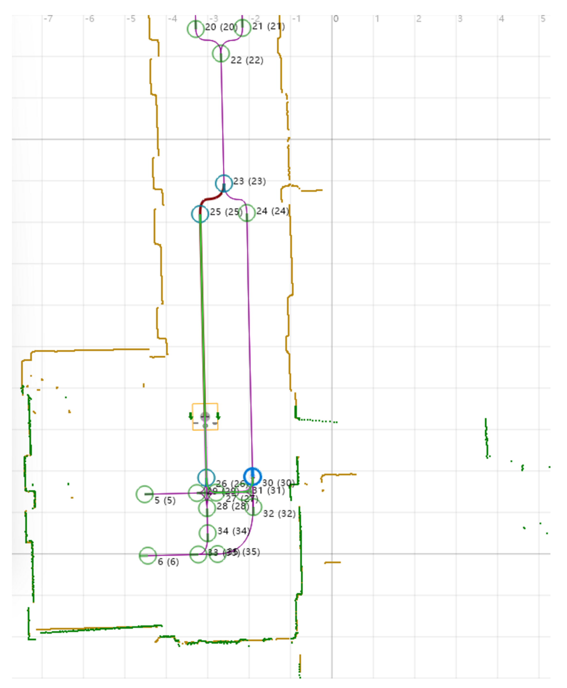

Table 1.
The results of constructing the shortest route.
| Agent | Found path | Stop reason | Number of visited cells | Remaining SoC | Travel time (conventional units) |
|---|---|---|---|---|---|
| 1 | (0, 4), (1, 4), (2, 4), (3, 4), (4, 4), (4, 3), (4, 2), (4, 1) | N/A | 8 | 0.400 | 7.20 |
| 2 | (0, 6), (0, 7), (1, 7), (2, 7), (3, 7), (4, 7), (5, 7), (6, 7), (7, 7), (8, 7), (9, 7) | N/A | 11 | 0.500 | 10.70 |
| 3 | (0, 3) | battery_low | 1 | 0.870 | 0 |
Table 2.
Comparison of different methods for finding shortest routes with constraints
| Method | Agent | Number of cells passed | Number of cells considered in order |
|---|---|---|---|
| Proposed | 1 | 8 | 61 |
| Proposed | 2 | 11 | 84 |
| Proposed | 3 | 12 | 97 |
| A* | 1 | 8 | 118 |
| A* | 2 | 11 | 74 |
| A* | 3 | 14 | 194 |
| Cooperative A* | 1 | 8 | 126 |
| Cooperative A* | 2 | 11 | 74 |
| Cooperative A* | 3 | 14 | 194 |
| M* | 1 | 8 | 25 |
| M* | 2 | 2 | None |
| M* | 3 | 12 | 34 |
| D* Lite | 1 | 10 | 67 |
| D* Lite | 2 | 11 | 19 |
| D* Lite | 3 | 14 | 33 |
| 1 | When the time index is clear from context or the environment state is fixed (e.g., during initial A* planning on a static snapshot), we write for brevity. |
| 2 | In algorithmic expressions, we write to denote the neighborhood of node u located at position , i.e., . |
Disclaimer/Publisher’s Note: The statements, opinions and data contained in all publications are solely those of the individual author(s) and contributor(s) and not of MDPI and/or the editor(s). MDPI and/or the editor(s) disclaim responsibility for any injury to people or property resulting from any ideas, methods, instructions or products referred to in the content. |
© 2026 by the authors. Licensee MDPI, Basel, Switzerland. This article is an open access article distributed under the terms and conditions of the Creative Commons Attribution (CC BY) license (http://creativecommons.org/licenses/by/4.0/).
Copyright: This open access article is published under a Creative Commons CC BY 4.0 license, which permit the free download, distribution, and reuse, provided that the author and preprint are cited in any reuse.


