

Submitted:
12 February 2026
Posted:
13 February 2026
You are already at the latest version
Abstract
Accurate prediction of student academic performance distributions is essential for institutional planning and decision support. This paper introduces a novel Monte Carlo (MC) framework for forecasting cohort-level grade distributions using historical data. The MC model extracts empirical probability distributions and generates predictions via stochastic sampling, explicitly capturing uncertainty and variability in student outcomes. Evaluated across engineering, medical, and aggregated student cohorts, the MC model outperformed a linear regression benchmark, particularly in capturing nonlinear grade transitions and stochastic variability. The MC approach preserves distributional structure and offers superior fidelity in modeling cohort behavior, serving as a reliable, uncertainty-aware complement to traditional machine learning. This work presents a validated probabilistic methodology and evaluation framework for predicting academic performance.
Keywords:
monte carlo
; simulation
; academic performance
; prediction
; probabilistic modeling
; distribution forecasting
; linear regression
; residual analysis
; uncertainty
; random number
1. Introduction
Predicting student academic performance has emerged as a key research area in Educational Data Mining (EDM) and Learning Analytics, motivated by the need to identify at-risk learners early, deliver personalized interventions, and improve educational outcomes. Accurate predictive models help institutions support timely decision-making, enhance student retention, and improve academic success rates in educational settings [1,2,3].
Student performance prediction typically entails forecasting future academic outcomes—such as grade point average (GPA), course grades, or pass/fail status—using information derived from demographic attributes, academic history, engagement indicators, and learning management system interactions [3]. A wide range of supervised machine learning techniques, including Decision Trees, Support Vector Machines, Random Forests, k-Nearest Neighbors, and Logistic Regression, have been extensively applied to this problem using structured student datasets [4,5,6]. Ensemble learning approaches often achieve higher accuracy by capturing nonlinear relationships among features; however, their performance remains sensitive to data imbalance, feature selection, and noisy or incomplete data.
Recent studies have explored advanced modeling paradigms such as deep neural networks, explainable learning frameworks, heterogeneous ensemble systems, and privacy-preserving federated learning approaches [7,8,9]. While these methods offer improved predictive performance in controlled settings, they typically assume deterministic data representations and produce point estimates without explicitly modeling uncertainty. Moreover, many deep models require large volumes of high-quality data and substantial computational resources, limiting their scalability and interpretability across diverse educational contexts.
These limitations motivate exploration of probabilistic and stochastic modeling frameworks capable of handling uncertainty, variability, and complex data distributions inherent in real-world educational systems. Here, Monte Carlo methods provide a theoretically grounded and computationally scalable alternative.
Monte Carlo algorithms constitute a broad class of randomized computational techniques that rely on stochastic sampling to obtain approximate numerical solutions to analytically intractable problems [10,11]. These methods are particularly effective in high-dimensional settings, where deterministic numerical techniques suffer from exponential computational growth, commonly referred to as the “curse of dimensionality.”
Monte Carlo methods estimate expected values and multidimensional integrals by averaging over randomly generated samples. Consider the estimation of the expectation of a measurable function :
where is a random variable with probability density function . When direct analytical evaluation is infeasible, independent samples are generated, and the Monte Carlo estimator is defined as
By the Law of Large Numbers (LLN), the estimator converges almost surely to the true expectation as . Furthermore, the Central Limit Theorem (CLT) guarantees asymptotic normality of the estimator, enabling statistical error analysis and confidence interval construction [11,12]. The root-mean-square error (RMSE) of the estimator decreases at a rate
which is independent of the dimensionality of the underlying problem. This property makes Monte Carlo methods particularly suitable for complex, high-dimensional systems.
A central challenge in Monte Carlo simulation is variance control, as high estimator variance slows convergence. Advanced variance-reduction techniques—such as importance sampling, control variates, and stratified sampling are commonly employed to improve efficiency and numerical stability [11,12]. These techniques have proven effective across domains involving uncertainty, including finance, engineering, and increasingly, predictive analytics.
In predictive modeling, Monte Carlo methods offer a distinct advantage by generating probabilistic forecasts rather than single deterministic predictions. By producing distributions of possible outcomes with associated likelihoods, Monte Carlo-based models provide richer insights into uncertainty and risk, which are essential for educational early-warning systems and academic decision support.
The main contributions of this paper are summarized as follows:
- Novel Monte Carlo Framework: We propose a Monte Carlo–based GPA prediction framework that explicitly incorporates probabilistic sampling, enabling reliable predictions under uncertainty and heterogeneous student data.
- Variance Reduction Techniques: The model integrates advanced variance-reduction strategies, improving convergence speed and stability for high-dimensional educational datasets.
- Comparative Evaluation: We evaluate the proposed framework using real-world datasets from PSAU’s engineering and medical faculties, demonstrating superior performance relative to state-of-the-art machine learning and deep learning models.
- Probabilistic Insight: Unlike deterministic predictors, the Monte Carlo model generates predictive distributions, providing actionable insights into uncertainty and risk in student academic outcomes.
- Scalability and Practical Deployment: The approach is computationally efficient and can be deployed in real educational settings, supporting early warning and targeted intervention systems.
The remainder of this paper is organized as follows. Section II reviews recent studies on student performance prediction. Section III presents the proposed Monte Carlo-based model. Section IV describes the experimental setup and evaluation metrics. Section V discusses the results and comparative analysis. Section VI concludes the paper and outlines recommendations for future research.
2. Previous Studies
While most research on predicting student performance traditionally relies on machine learning algorithms such as Support Vector Machines (SVM), decision trees, and linear regression , recent studies continue to corroborate the effectiveness of these approaches in educational contexts. For example, a recent systematic review highlights the extensive use of classical ML models (e.g., SVM, decision trees, logistic regression) for forecasting academic success and identifying at-risk students, demonstrating that such models often achieve high classification accuracy and enable early interventions based on behavioral and institutional attributes [13]. Empirical studies further show the effectiveness of these techniques: classification algorithms, including Random Forests, SVM, and nearest neighbors, have been successfully applied to predict student exam performance, helping institutions identify students who are likely to succeed or fail [14]. Additional research confirms that both traditional ML and deep learning models (e.g., neural networks) provide consistent performance prediction when evaluated on real academic datasets [15].
In contrast, although Monte Carlo methods have been extensively applied across a wide range of domains, including physics (as examples [16,17]), finance (as examples [18,19]), engineering (as examples [20,21]), healthcare (as examples [22,23]), and risk analysis (as examples [24,25,26]). Their adoption in the field of educational data mining remains limited. In particular, relatively few studies have explicitly employed Monte Carlo methods for predicting students’ performance outcomes, as in [27,28,29,30,31].
In [27], the authors develope a Monte Carlo simulation predictive model that allows prospective students to estimate the number of applicants to the Department of Hadith Sciences for the upcoming academic year. The research technique employed in this study uses a Monte Carlo simulation to apply this research. The number of students in the Department of Hadith Sciences who enrolled from 2019 to 2023 serves as the data used to predict the number of new student registrations. They develop a simulation system to forecast the number of new applicants to the Hadith Sciences program using the classical simulation methodology.
In [28], the authors develop a generic computer-based tool that uses Monte Carlo stochastic simulation and historical data to analyze and predict student performance within a given curriculum. They model subject completion as a sequence of probabilistic events; their model computes critical metrics defined by Spain's National Quality Evaluation and Accreditation Agency (ANECA), specifically the graduation rate (students finishing on time or with one extra year) and the efficiency rate (the ratio of required to actual credits taken). They design an experiment to test how changes in regulations, such as the maximum number of credits a student can enroll in, affect overall success before implementing new curricula. Unlike previous studies focused on individual students, this simulator provides a "workshop" to optimize entire academic programs and identify which features most influence indicators, as demonstrated by its specific application to the Bachelor in Engineering Technologies at the Technical University of Madrid
In [29], the authors examine factors that may affect students' motivation to learn scientific computing in the undergraduate systems engineering program at the University of Córdoba (Colombia). They conducted a survey of 117 students and then applied multidimensional linear regression to identify a function that captures the regular patterns associated with motivation and its influencing factors. They used the Monte Carlo method in exploring the multidimensional space of independent variables to estimate the probability that a student attains one of ten motivation levels, ranging from completely demotivated to highly motivated to learn scientific computing.
In [30], the authors examine the divergent mechanisms by which teachers' support for students affects students' performance on low- and high-stakes assessments. They used Bayesian structural equation modeling (BSEM) with the Markov Chain Monte Carlo (MCMC) algorithm to evaluate the structural relationships among teacher support, student behavior, and [formative and summative] academic performance. We also assessed moderated relationships, focusing on students' gender and interactions with teacher support. They used Bayesian structural equation modeling with the Markov Chain Monte Carlo algorithm and Ghanaian data to capture the cumulative nature of student learning and performance assessment. They evaluated student performance during daily schooling (formative assessment) and at the end of their academic program (summative assessment).
In [31], the authors study factors that can affect student performance in online learning by developing an empirical model. They tested the reliability of their model linguist reviews using construct reliability coefficients and confirmatory factor analysis (CFA), and a one-sample Kolmogorov-Smirnov test with the Monte Carlo method.
3. The Model
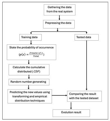
Figure 1 presents the proposed Monte Carlo–based framework for predicting student performance. The model follows a structured pipeline that begins with data acquisition from the real educational system and proceeds through probabilistic modeling, stochastic simulation, and performance evaluation. Each stage of the model is designed to capture the uncertainty inherent in student behavior and academic outcomes.
3.1. Data Collection from the Real System
The first stage of the proposed model involves gathering raw data from the real educational environment. This dataset includes historical records related to students’ academic performance, such as assessment scores, course completion status, and other relevant academic indicators. The collected data serve as the empirical foundation upon which the probabilistic model is constructed.
3.2. Data Preprocessing
Before probabilistic modeling, the raw data undergoes preprocessing to ensure consistency, completeness, and suitability for analysis. This step includes handling missing values, removing outliers, and transforming variables where necessary. The preprocessed dataset is then divided into two subsets: a training dataset, used to estimate the underlying probability distributions, and a testing dataset, reserved exclusively for evaluating model performance.
The training data are used to construct the probability model and perform Monte Carlo simulations, while the testing data remain unseen during training to provide an unbiased evaluation of predictive accuracy. This separation ensures that model validation reflects real-world predictive performance.
3.3. Probability of Occurrence Estimation
Using the training dataset, the probability of occurrence for each observed outcome is estimated empirically. Let denote a discrete random variable representing a student performance metric. The probability mass function is computed as:
This empirical probability estimation captures the observed distribution of student outcomes without imposing parametric assumptions.
3.4. Cumulative Distribution Function Construction
Based on the estimated probabilities, the cumulative distribution function (CDF) is constructed. The CDF is defined as:
The CDF plays a central role in the Monte Carlo simulation process, as it enables the transformation of uniformly distributed random numbers into samples that follow the empirical distribution of student performance [32]
3.5. Random Number Generation
Random number generation constitutes a core component of the proposed Monte Carlo–based simulation framework. At this stage, pseudo-random numbers uniformly distributed over the interval are generated and used as stochastic inputs for sampling from the empirical cumulative distribution function (CDF) of student performance.
In computational simulations, true randomness is typically approximated using pseudo-random number generators (PRNGs), which produce deterministic sequences of numbers that exhibit statistical properties consistent with independent realizations from a target distribution. Most modern PRNGs are designed to generate sequences that closely approximate the continuous uniform distribution over , making them suitable for Monte Carlo simulation and probabilistic modeling tasks [33,34]
Let be a random variable uniformly distributed on the unit interval, i.e. :
Accordingly, a sequence of independent pseudo-random numbers is generated, where each represents a stochastic realization. These values serve as inputs for inverse CDF sampling from the empirical distribution of student performance outcomes.
From an algorithmic perspective, a wide range of well-established PRNGs exist for generating uniform random numbers, including Linear Congruential Generators (LCGs), Mersenne Twister, Xorshift, and Permuted Congruential Generators (PCG). These algorithms differ in terms of period length, equidistribution properties, and computational efficiency. However, contemporary scientific programming environments and software platforms (e.g., MATLAB, Python, R, Java) implement high-quality PRNGs by default, which have been extensively validated for Monte Carlo applications.
Since the proposed model relies exclusively on uniformly distributed pseudo-random numbers and does not require specialized stochastic properties beyond uniformity and independence, the internal PRNG provided by the software environment is sufficient. Therefore, the design of a custom random number generation algorithm is outside the scope of this work. The focus instead is placed on how the generated uniform samples are transformed via the empirical CDF to model uncertainty in student performance predictions.
3.6. Monte Carlo Prediction via Distribution Transformation
The generated random numbers are mapped to predicted student performance values using inverse transformation and empirical distribution techniques. By repeatedly sampling from the CDF, the model produces a large number of simulated outcomes, thereby estimating the probabilistic behavior of student performance under uncertainty. This Monte Carlo process allows the model to generate predictions that reflect variability and uncertainty rather than single-point estimates.
To transform the uniformly distributed random variables into samples following the empirical distribution of student performance, the inverse cumulative distribution function (inverse CDF) method is employed [34,35] as follows:
Let denote the cumulative distribution function of the discrete random variable , constructed from the training data as:
The inverse CDF, also known as the quantile function, is defined as:
A simulated student performance value is then obtained by:
By repeatedly applying this transformation for a large number of samples , the model generates a set of simulated outcomes:
These simulated values approximate the empirical distribution of student performance and enable probabilistic prediction under uncertainty.
3.7. Model Evaluation and Result Analysis
The model outcomes are then compared with the testing dataset to assess predictive performance through a designed and implemented experiment. Evaluation metrics such as prediction error, distributional similarity, or classification accuracy (depending on the application context) are computed. This comparison quantifies the model’s ability to generalize beyond the training data. The final output of this stage represents the evaluation results, which indicate the effectiveness of the proposed Monte Carlo–based prediction model.
The expected predicted performance can be estimated as:
while the variability of predicted outcomes is captured by the sample variance:
This formulation allows the proposed model to provide not only point predictions but also uncertainty-aware estimates of student performance.
Beyond experiment-specific diagnostics, a broader evaluation is conducted through a benchmark to assess the overall predictive capability of the proposed modeling framework relative to deterministic alternatives.
4. Experimental Setup and Evaluation
The proposed model was implemented in Python. We used Python because it is a widely adopted, high-level, interpreted programming language that supports scientific computing and data analysis. Owing to its extensive ecosystem of numerical and statistical libraries, it makes it an effective and flexible environment for implementing Monte Carlo simulations and probabilistic modeling techniques[36,37].
This section details the experimental design and implementation of the proposed model. Specifically, it describes the dataset characteristics, the preprocessing and data transformation procedures, and the key implementation details, while ensuring consistency with the model framework introduced in Section 3.
4.1. Dataset Description
The dataset used in this study consists of real academic records collected from the Primary Year program at Prince Sattam bin Abdulaziz University (PSAU) over two consecutive academic years: 2015/2016 () and 2016/2017 (). In the primary year, there are two major disciplines: one for students who decide to study engineering and science, and the other for students who decide to study medicine and medical science. The total number of students in the academic year was 1224 students (675 in the engineering discipline and 537 in the medical science discipline), while the total number of students in the academic year was 959 students (554 in the engineering discipline and 405 in the medical science).
To evaluate the predictive capability of the proposed model, the dataset was temporally partitioned. Records from the academic year were used to construct the empirical distributions required by the model (training phase), while data from the academic year were reserved for testing and validation. This split reflects a realistic deployment scenario in which historical academic data are used to predict future student outcomes. In addition, we will train and test our model on 3 categories of datasets: individual-discipline datasets and the entire dataset.
In the PSAU Primary Year system, students complete two academic semesters, after which their Grade Point Average (GPA) is computed. This GPA determines eligibility and placement into specific colleges, making it a critical variable for both students and academic administrators. Consequently, accurate modeling of GPA-related outcomes is essential for informed decision-making, academic planning, and early intervention strategies.
The dataset comprises all student data during this year, including the final GPA attributes, making it well-suited for assessing the flexibility of the proposed probabilistic model in handling heterogeneous data types.
Table 1 presents a sample of part of the original dataset after de-identifying the data to protect student privacy.
4.2. Data Preprocessing
Data preprocessing was performed to align the raw academic records with the requirements of the proposed Monte Carlo simulation framework. At this stage, student records were organized and categorized according to academic performance levels.
Specifically, students were grouped into six discrete grade categories based on GPA ranges defined by the Primary Year academic regulations. Each GPA value was mapped to a corresponding grade label. This discretization step serves two purposes:
- It reduces continuous GPA values into interpretable performance classes, and
- It facilitates the construction of empirical probability distributions required for Monte Carlo sampling.
To demonstrate the model’s capability to process both numerical and textual representations, grade information was retained in textual form while preserving numerical GPA values for computation. Frequency counts for each grade category were then calculated.
The preprocessing algorithm, illustrated in Figure 2, is responsible for transforming raw academic data into a structured form suitable for probabilistic modeling. The process begins by reading the cleaned dataset from an Excel file and extracting the Grade Point Average (GPA) values into a one-dimensional array.
Let the set of GPA values be defined as:
where denotes the total number of students.
The GPA values are optionally sorted to support descriptive analysis and distribution inspection.
Each GPA value is then classified into a discrete grade category based on predefined institutional thresholds using an iterative conditional structure. The classification rule is formally defined as:
4.3. Data Transformation and Probabilistic Modeling
Following preprocessing, the dataset was transformed into a probabilistic representation compatible with the Monte Carlo model process described in Section 3.
For each grade category, the probability of occurrence was computed by dividing its frequency by the total number of students. Based on these probabilities, the cumulative distribution function (CDF) was constructed. The CDF provides a monotonic mapping between uniformly distributed random numbers and grade categories, enabling inverse transform sampling.
Additionally, random-digit intervals were assigned to each grade according to cumulative probability ranges. These intervals define the mapping rule by which a generated uniform random number is associated with a specific grade outcome. This transformation step is essential for translating stochastic realizations into predicted academic performance categories.
The processing algorithm, shown in Figure 3, converts the grade frequencies obtained during preprocessing into a probabilistic representation. Let represent the frequency of grade category , where:
The probability of occurrence for each grade is computed as:
These probabilities form a discrete probability distribution:
To enable Monte Carlo predicting mode, the cumulative distribution function (CDF) is computed as:
This cumulative probability array defines the random digit assignment intervals, mapping uniformly distributed random values to discrete grade outcomes
4.4. Predicting the Students’ Performance
The prediction stage, illustrated in Figure 3, applies the probabilistic model constructed in the previous steps. Pseudo-random numbers uniformly distributed over the interval [0,1] were generated using Python’s built-in random number generator.
Each generated random value was compared against the predefined random-digit intervals obtained from the empirical cumulative distribution function (CDF). Based on this comparison, the value was mapped to its corresponding grade category, yielding a single predicted GPA. This process was repeated iteratively so that the total number of generated GPA values equaled the number of students in the test dataset, ensuring a one-to-one correspondence between predicted and observed student records during model evaluation.
In accordance with the prediction algorithm illustrated in Figure 3, the model was evaluated using three distinct test datasets representing different student populations: engineering students, medical students, and the entire student cohort. This experimental design enables an assessment of the model’s predictive behavior across academically diverse groups. Repeated application of this algorithm yielded a set of predicted GPAs and an overall simulated distribution of student performance outcomes. Table 7 presents representative samples of the predicted grades generated through this procedure, and Table 8 the final model predicted grade compared with the actual results.
4.5. Experimental Evaluation
This section evaluates the outcomes of the experiment by examining the agreement between the predicted and observed grade distributions produced by the proposed model. The evaluation is organized into two complementary components. First, global agreement is quantified using distribution-based error metrics and goodness-of-fit measures that capture the overall similarity between predicted and empirical distributions. Second, residual diagnostics are performed to investigate category-level deviations and identify localized prediction behavior.
4.5.1. Distributional Evaluation and Error Metrics
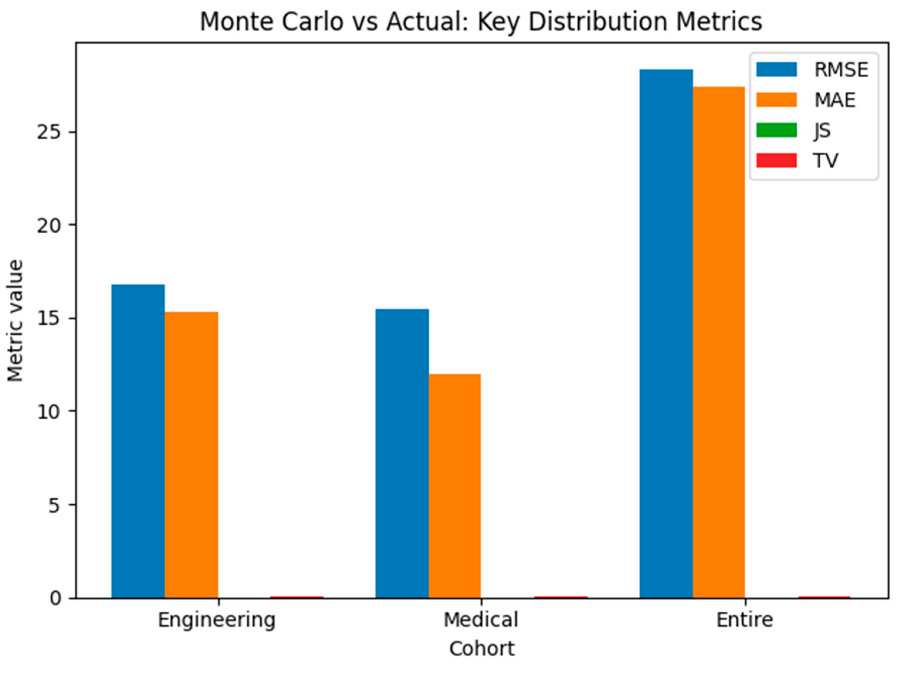
Agreement between predicted and observed distributions is quantified using count-based errors (RMSE and MAE) and distribution-level similarity measures. The Chi-square goodness-of-fit statistic tests whether predicted counts are consistent with observed counts. Distribution distances include KL divergence (Actual || Predicted), Jensen–Shannon divergence (JS), total variation distance (TV), and Bhattacharyya distance. Lower error/distance indicates closer agreement; for Chi-square, a larger p-value indicates a closer fit. Table 9 presents the distribution-level evaluation metrics (Monte Carlo vs. actual), while Figure 4 and Figure 5, and 6 visualize predicted and observed grade distributions for each cohort. Figure 7 and Figure 8, and 9 overlay plots that highlight distribution-shape agreement, and Figure 10 provides direct category-level comparisons in a bar chart.
Figure 4.
Engineering Students: Predicted vs. actual grade distribution (overlay).
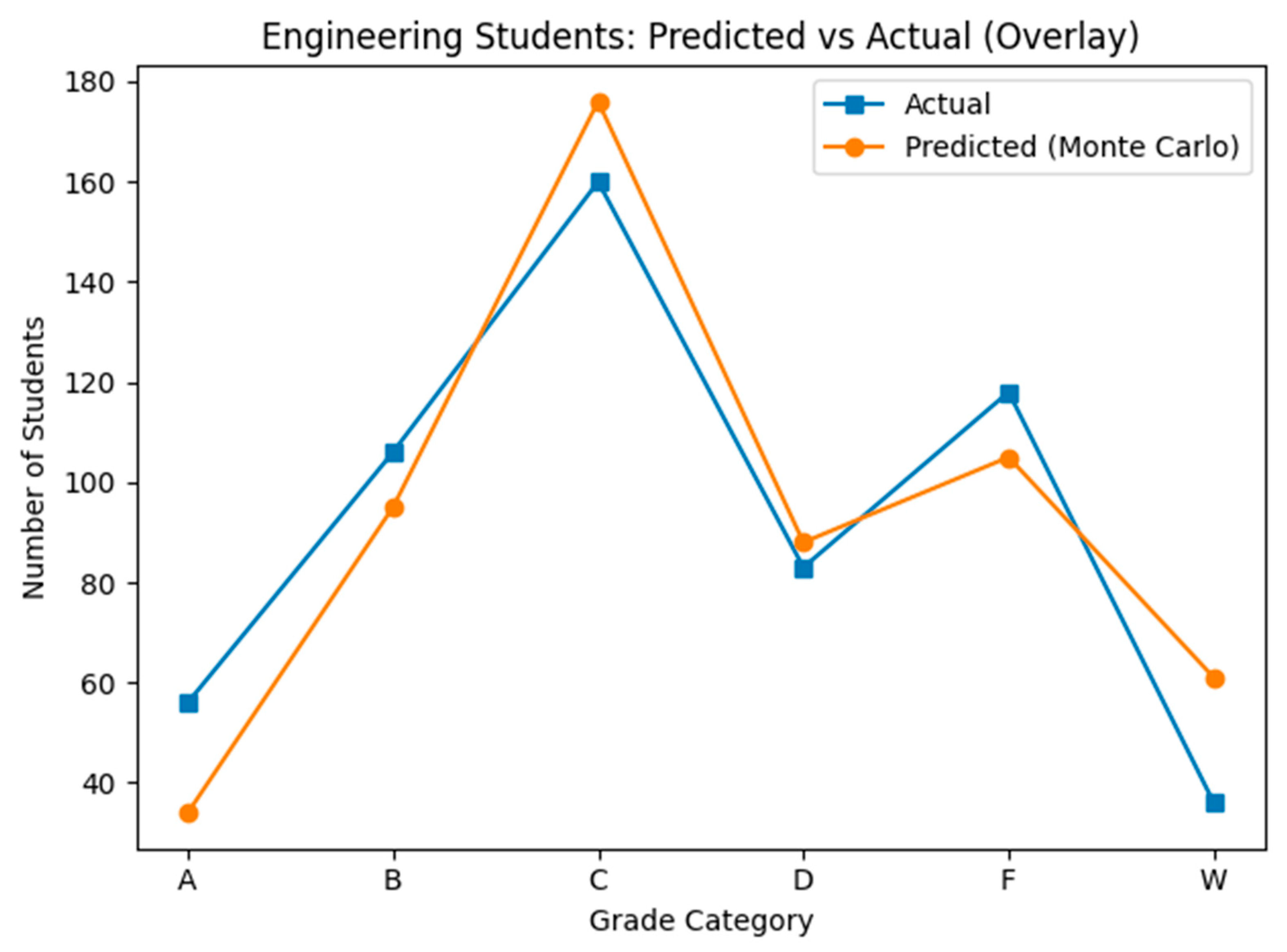
Figure 5.
Medical Students: Predicted vs. actual grade distribution (overlay).
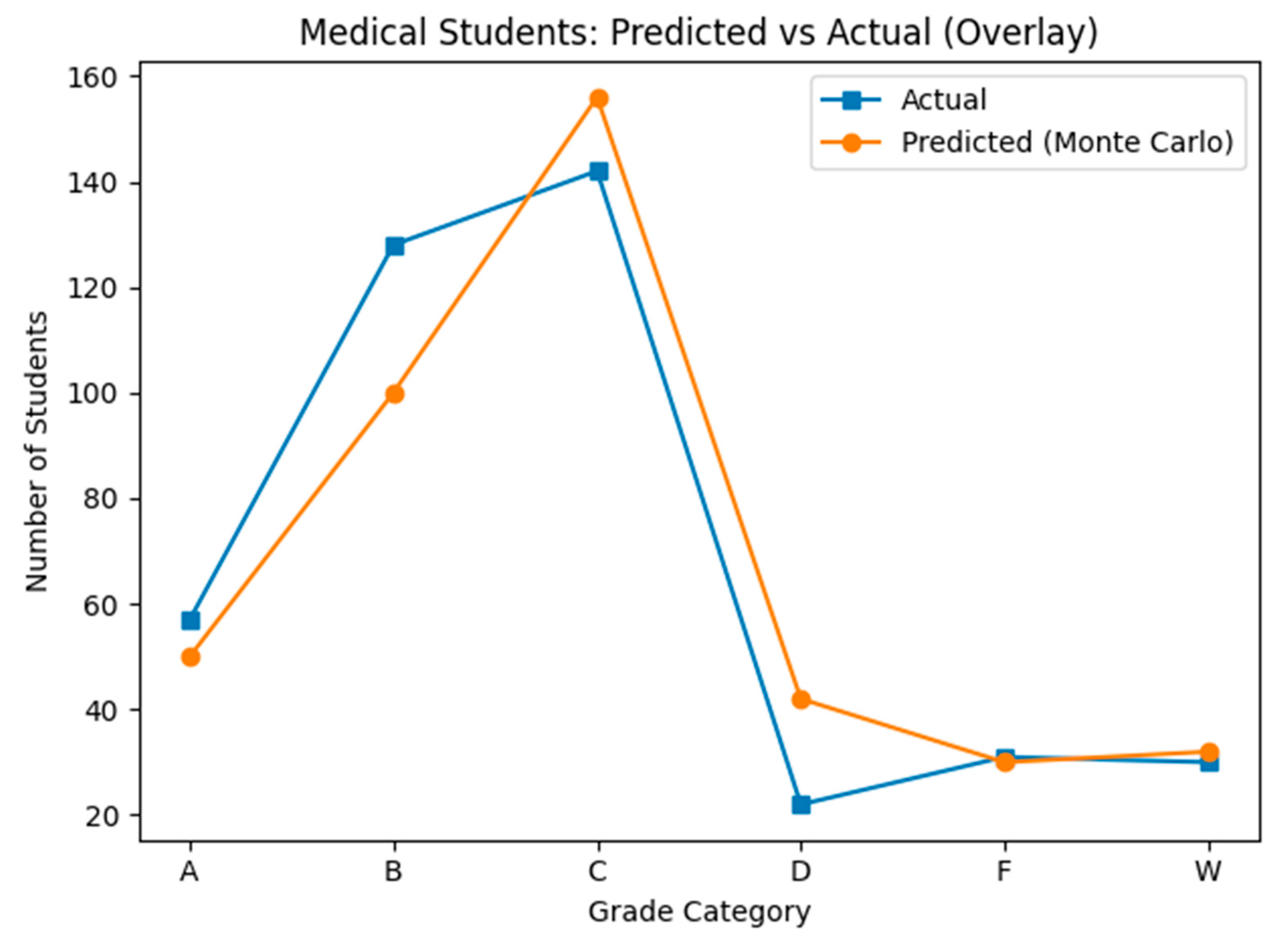
Figure 6.
Entire Students: Predicted vs. actual grade distribution (overlay).
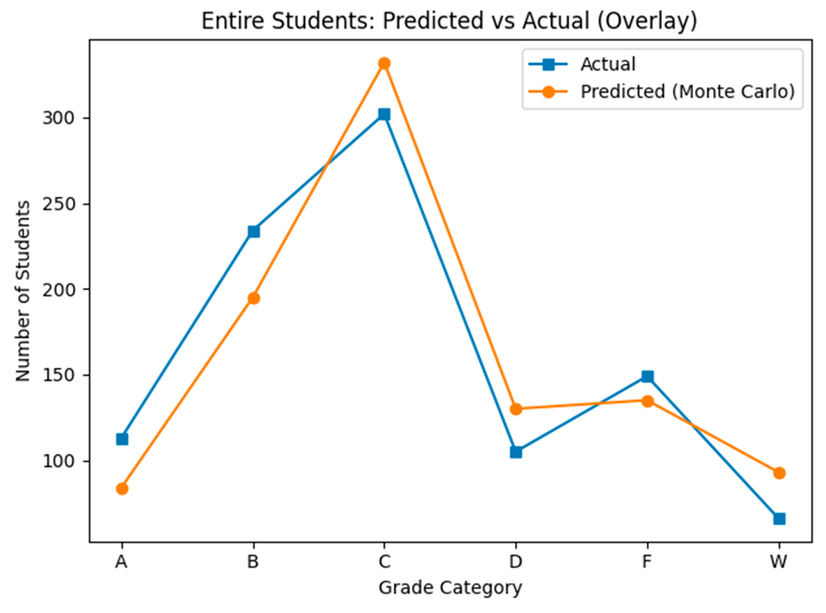
Figure 7.
Engineering Students: Predicted vs. actual grade distribution (bar chart).
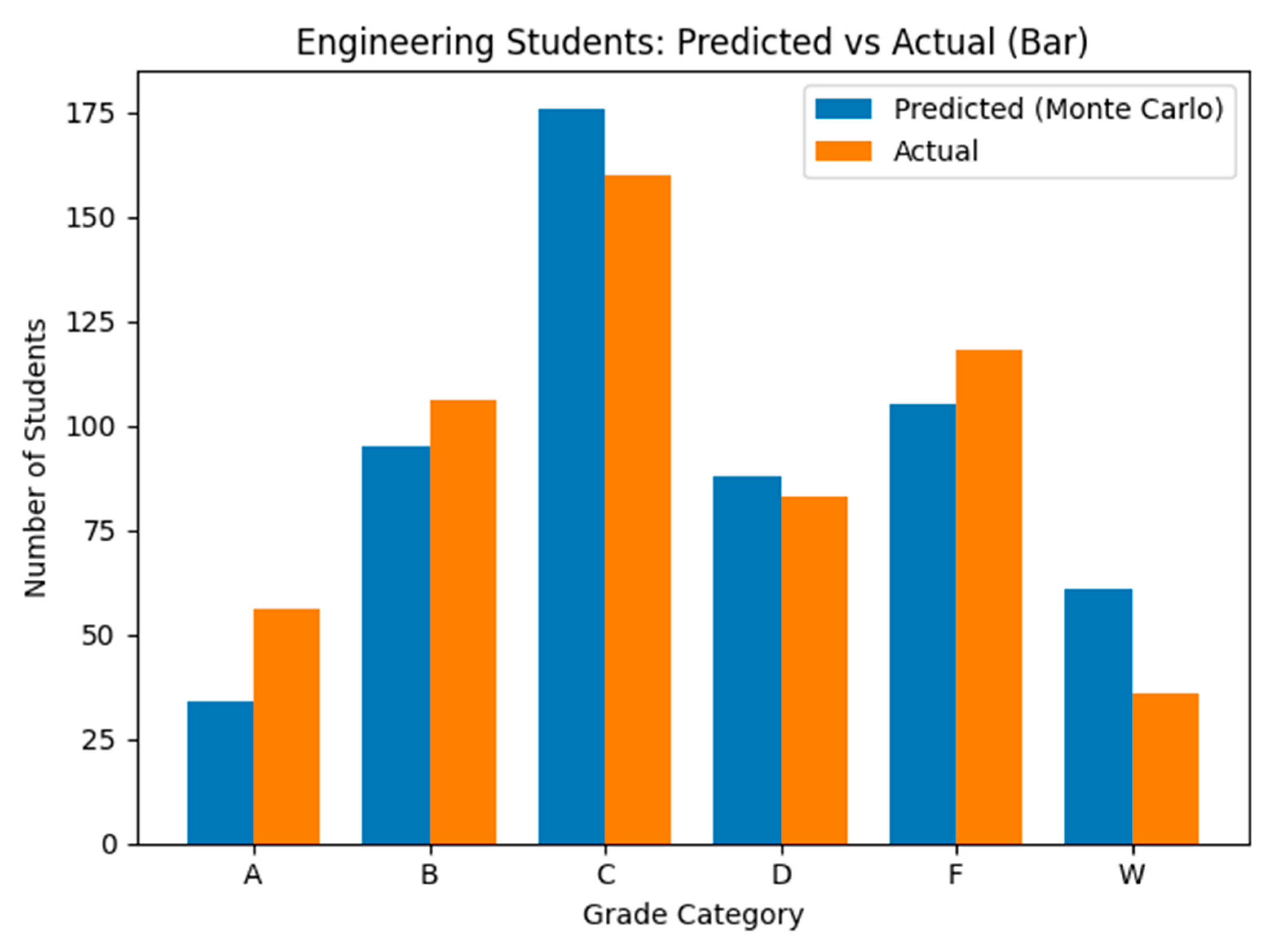
Figure 8.
Medical Students: Predicted vs. actual grade distribution (bar chart).
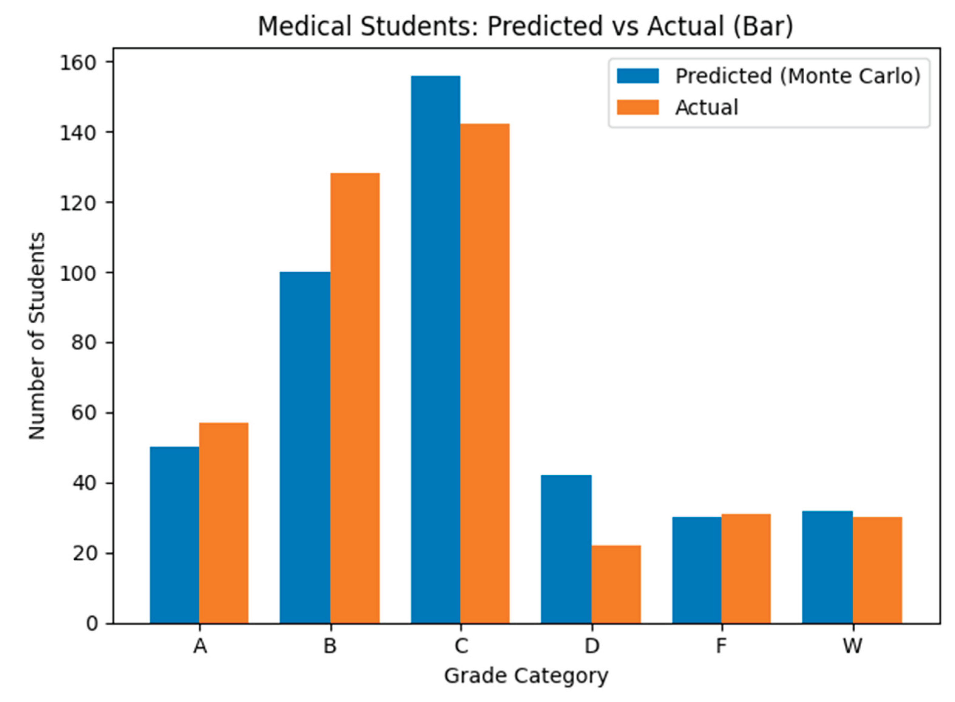
Figure 9.
Entire Students: Predicted vs. actual grade distribution (bar chart).
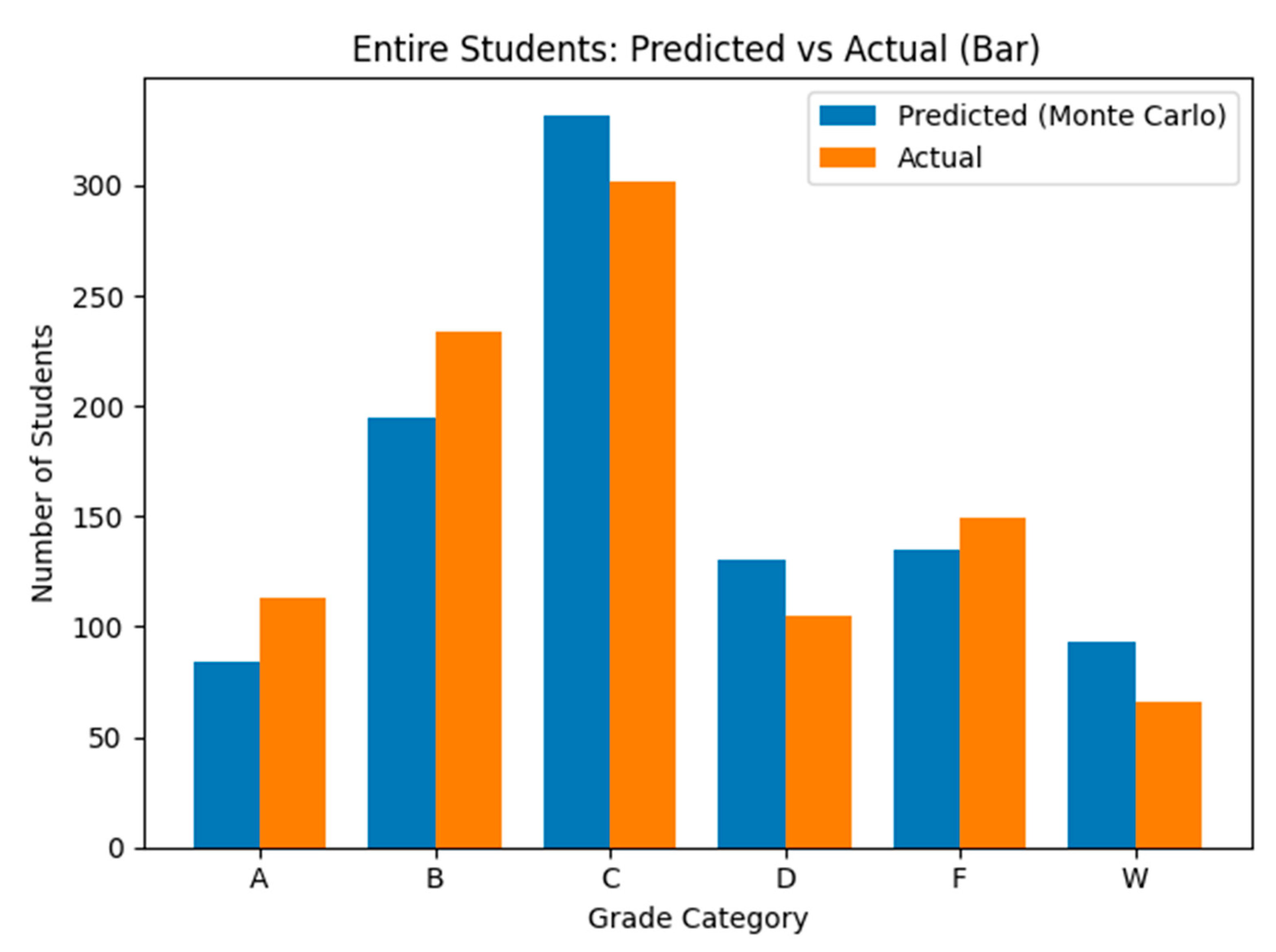
Figure 10.
Summary of key distribution metrics across cohorts.
4.5.2. Residual Analysis and Diagnostic Assessment
To ensure that the model has captured the underlying data patterns and that the remaining error is merely random noise, residuals were computed per grade category as:
Where:
is residual (The remaining error is merely random noise
is the actual value and
Figure 11.
Engineering Students: Residual plot (Actual − Predicted).
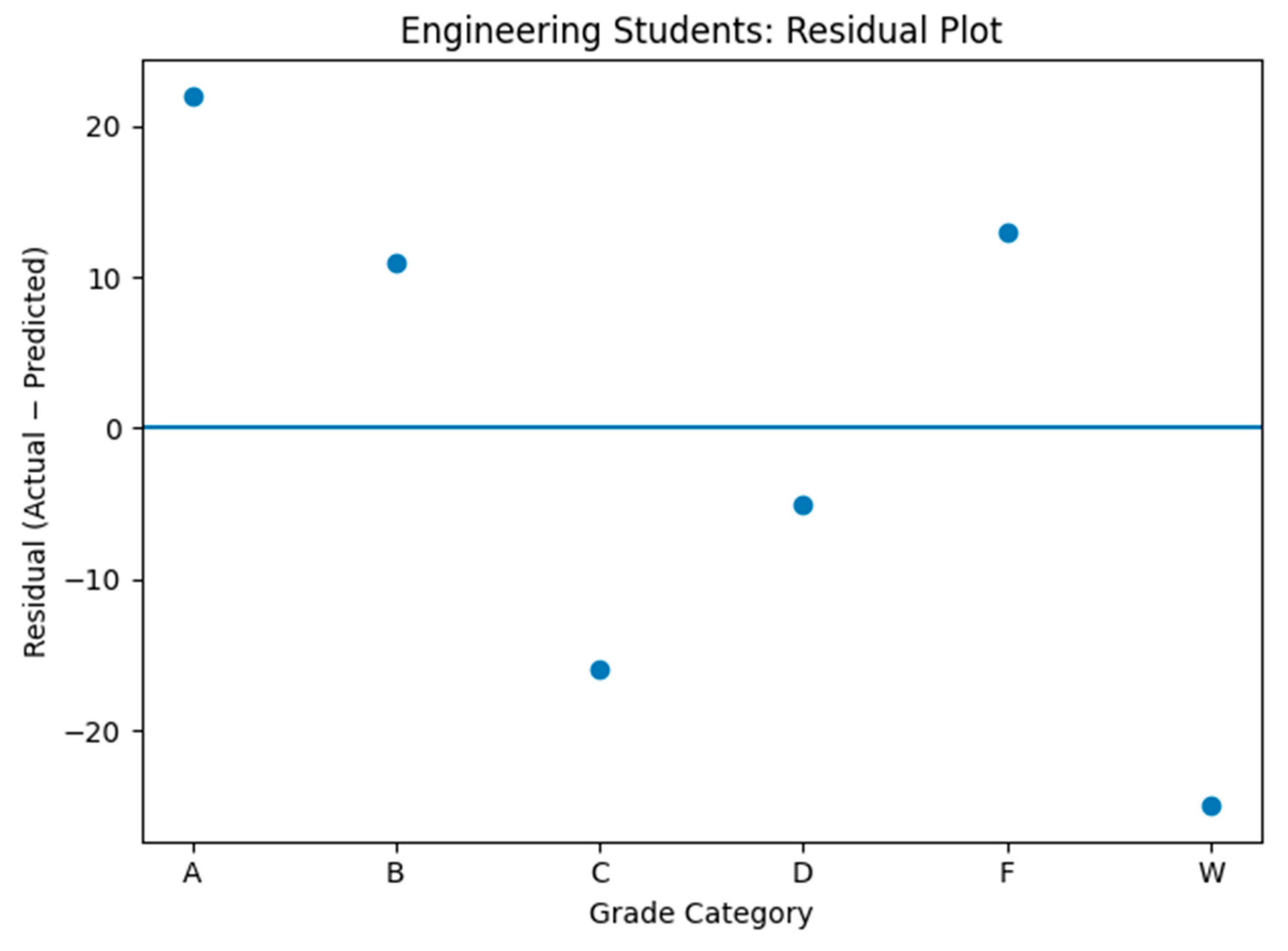
Figure 12.
Engineering Students: Residual plot (Actual − Predicted).
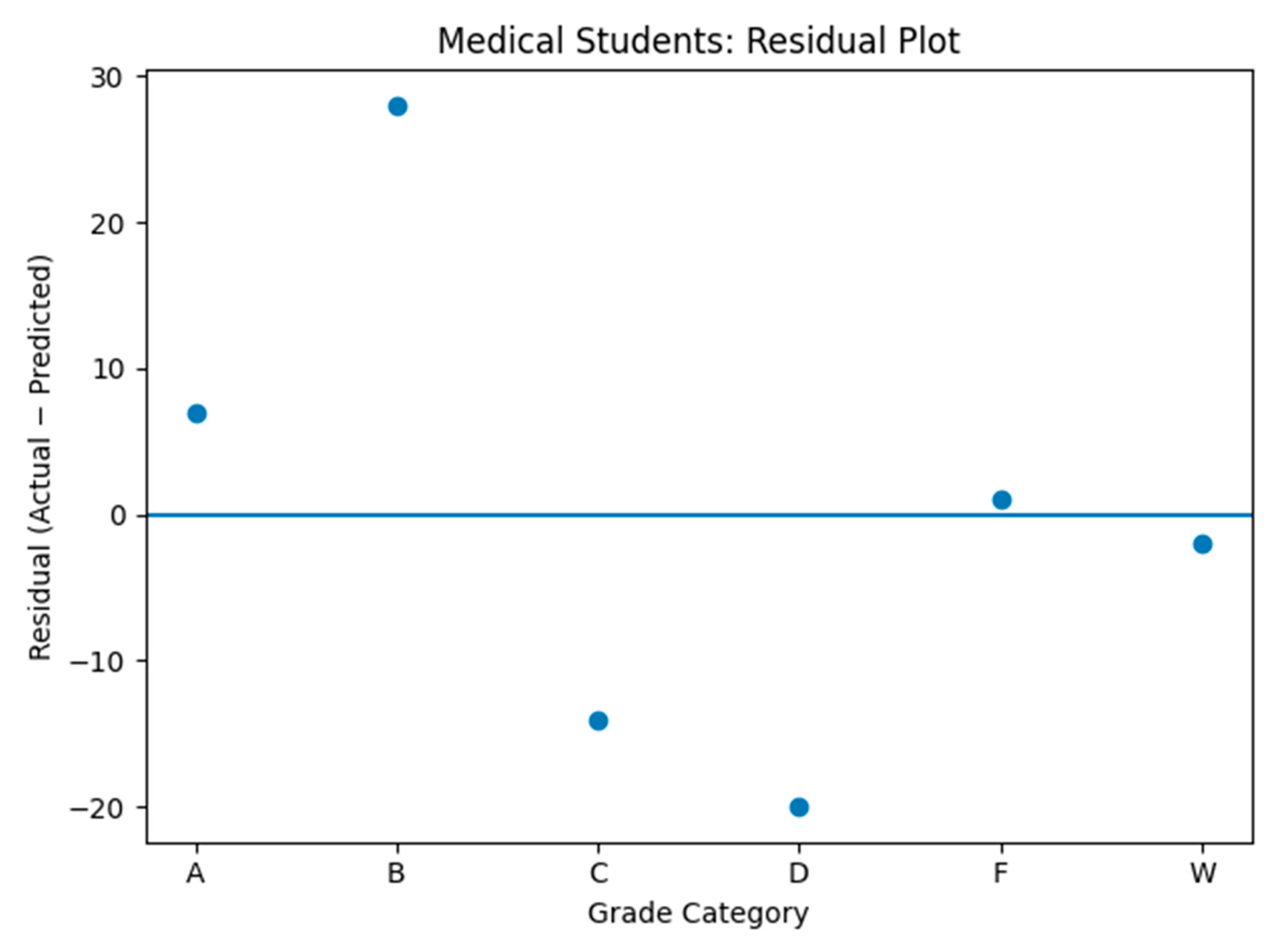
Figure 13.
Entire Students: Residual plot (Actual − Predicted).
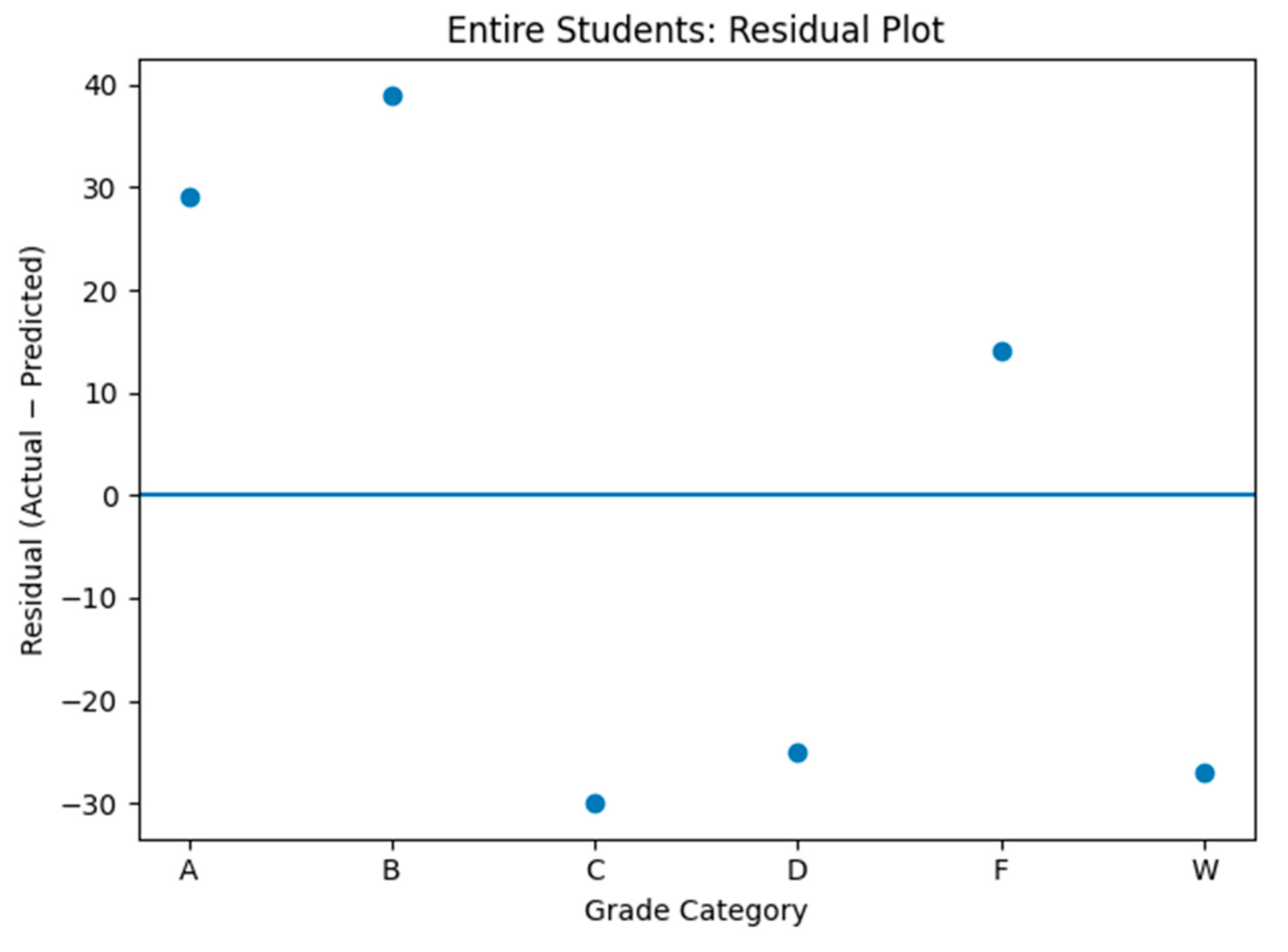
Table 10 presents the analysis results. Positive residuals indicate underprediction by the model, while negative residuals indicate overprediction. Residual plots provide a diagnostic view of where the model deviates from the observed distribution (see Figures 11,12, and 13).
Residual analysis is a critical diagnostic method in statistics and machine learning used to evaluate the appropriateness of a model by analyzing the residuals—the differences between observed values and values predicted by the model. It checks key assumptions like linearity, constant variance (homoscedasticity), and independence of errors. A random pattern in residual plots indicates a good fit, while structured patterns suggest model deficiencies [38].
Normality of residuals was assessed using the Shapiro–Wilk test [39]. Since all p-values exceed 0.05, the null hypothesis of normality cannot be rejected, implying that deviations are consistent with stochastic variation rather than structural model misspecification. Bias and balance evaluation based on residual sign symmetry and zero mean indicates calibrated probabilistic interval construction and stable stochastic sampling behavior.
Residual magnitudes are concentrated primarily in extreme and transition grade categories, which is expected in Monte Carlo sampling due to the higher variability associated with low-probability outcomes. No systematic clustering or directional drift was observed. These findings indicate that the empirical probability representation captures the underlying distribution adequately.
Overall, diagnostic assessment confirms statistical neutrality, absence of bias, and residual patterns consistent with well-behaved stochastic simulation models, reinforcing confidence in the proposed probabilistic forecasting framework.
4.5.3. Results Discussion
The Monte Carlo model captures the overall distributional structure across cohorts while exhibiting cohort-dependent deviations in specific grade categories. Engineering students show the largest absolute deviations in the A and W categories, which typically have lower frequency and higher relative variability. Medical students show pronounced deviations in the B, C, and D categories, reflecting distributional drift between academic years. For the entire cohort, aggregation amplifies mid-range category deviations (C and D), consistent with heterogeneous subgroup behavior. Residual diagnostics identify the dominant error contributors and can guide refinement of empirical probabilities and interval assignment.
The evaluation results demonstrate that the proposed model effectively captures the probabilistic structure of student performance outcomes. By relying on empirical distributions and stochastic sampling, the model provides a realistic representation of uncertainty that is often overlooked by deterministic prediction approaches.
These findings suggest that Monte Carlo–based modeling constitutes a viable and interpretable alternative for academic performance prediction, particularly in scenarios where uncertainty, variability, and limited data availability play a critical role.
5. Model Evaluation
To evaluate the proposed Monte Carlo simulation framework, a linear regression baseline will be adopted rather than more complex machine-learning algorithms because:
- The available datasets consist of aggregated grade-frequency counts rather than individual-level feature vectors; applying instance-level machine-learning classifiers to aggregated data risks introducing ecological inference bias, whereby relationships observed at the group level may not hold at the individual level [40].
- Regression at the aggregate level remains appropriate when the target of inference is group-level behaviour rather than individual prediction, as parameters estimated from aggregated observations may still provide valid insights about aggregate outcomes when interpreted consistently with the data level [41]. This ensures methodological alignment between the Monte Carlo model output (distribution predictions) and the comparator model output.
- Simple linear models are widely accepted as interpretable and computationally efficient baselines in predictive modelling, providing transparent parameterization and diagnostic insight before introducing additional complexity. Empirical evidence demonstrates that simpler linear approaches may rival or outperform more complex machine-learning techniques in certain applied settings while offering clearer interpretability and reduced computational cost. Moreover, rigorous evaluation practice emphasises the importance of selecting appropriate baseline models and metrics to avoid misleading conclusions regarding model generalizability and performance [42].
Taken together, these considerations justify the use of linear regression as a principled baseline for evaluating the Monte Carlo model. The regression benchmark provides an interpretable deterministic reference operating in the same aggregated output space, allowing performance improvements attributable to stochastic simulation to be assessed without introducing methodological inconsistencies or ecological inference bias.
5.1. Implementing the Linear Regression Prediction Model
In this section, a linear regression predictor will be implemented as a deterministic benchmark for the proposed Monte Carlo simulation model. Both approaches are evaluated in the same output space (cohort-level grade-frequency distributions). Using Table 2 (section 4) as the training dataset (Y₁) and Table 3 (section 4) as the test dataset (Y₂), the benchmark learns a mapping from Y₁ grade counts to Y₂ grade counts and predicts the expected distribution in the subsequent year. Figure 14 shows the algorithm used for implementing the Linear Regression Prediction Model.
For each cohort, an ordinary least squares (OLS) linear regression model is fitted at the grade-category level as:
where denotes the observed grade frequency in Year 1, is the predicted grade frequency in Year 2, α is the slope coefficient, and β is the intercept. Parameters are estimated by minimizing the squared error over grade categories.
5.2. Results, Evolution, and Comparisons
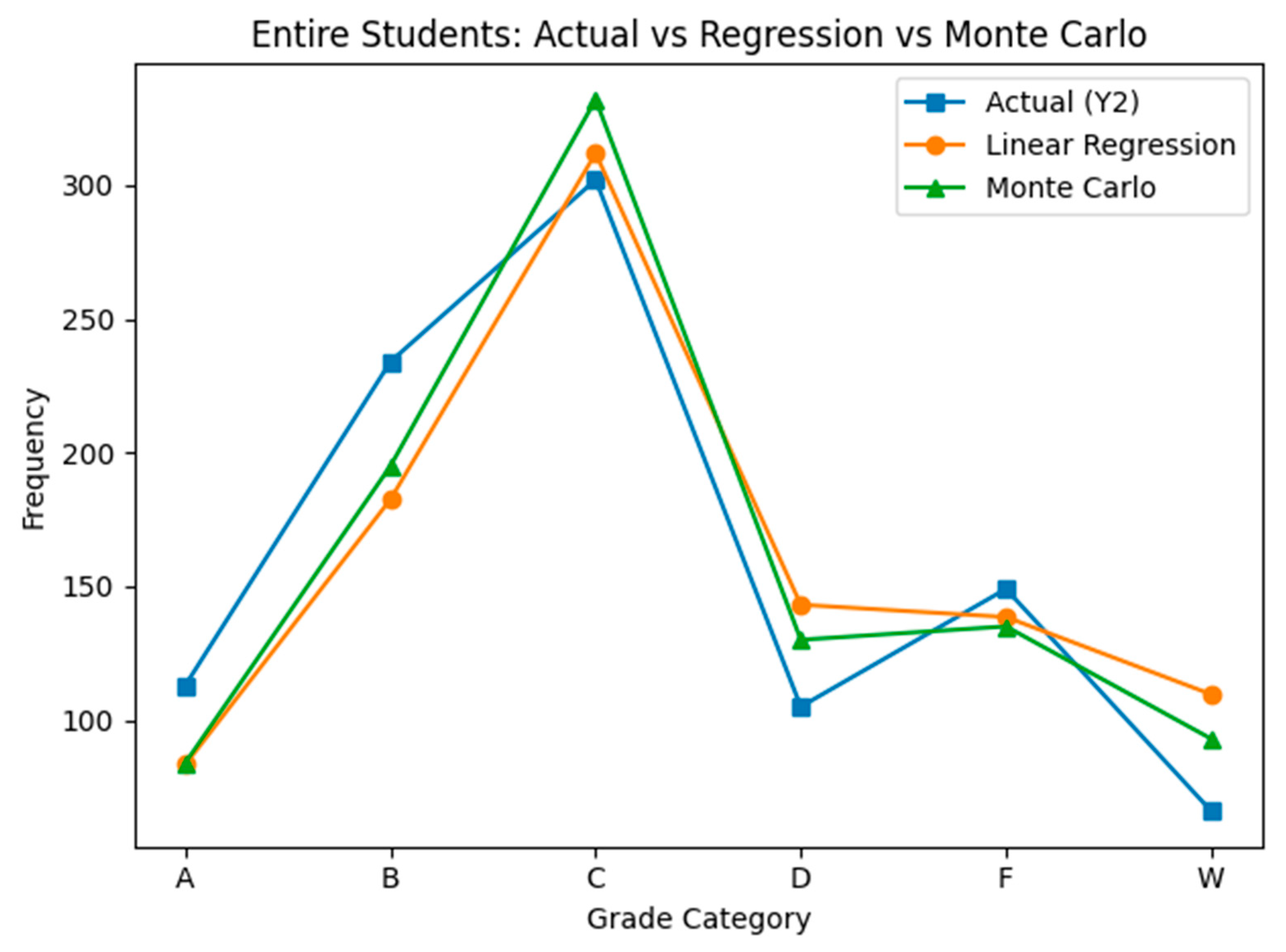
Table 11 presents training (Y₁), test (Y₂), and model prediction results (Regression and Monte Carlo), and Figure 15 and Figure 17, and 18 visualizing these results
Figure 15.
Engineering Students: Linear Regression vs Monte Carlo.
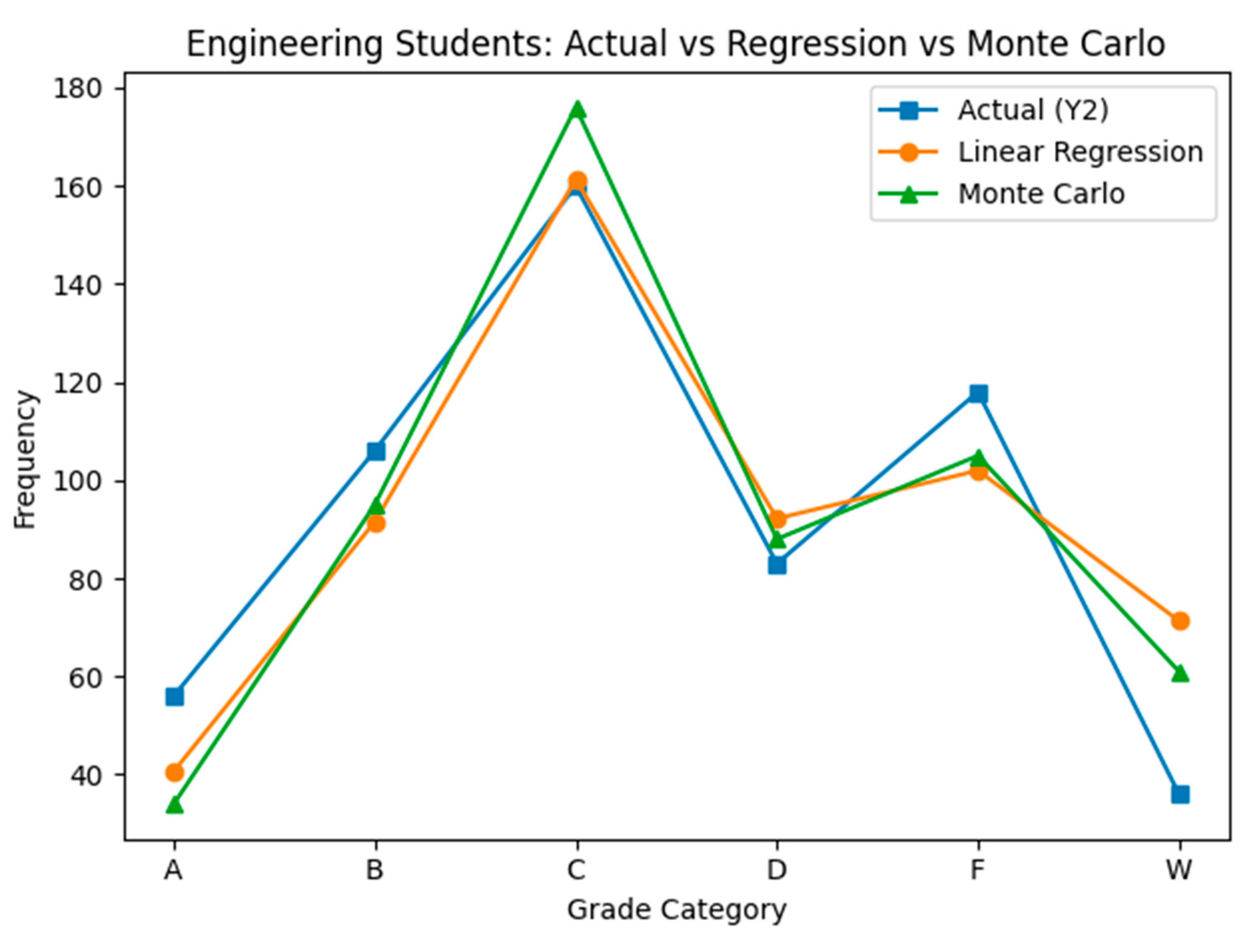
Figure 16.
Medical Students: Linear Regression vs Monte Carlo.
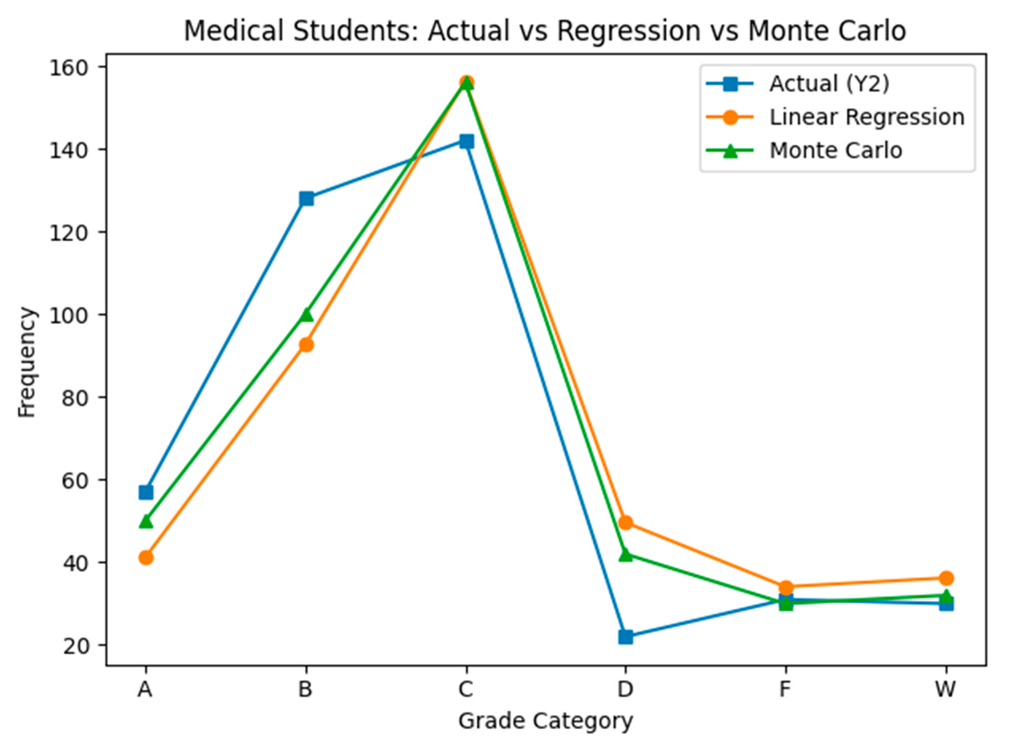
Figure 17.
Entire Students: Linear Regression vs Monte Carlo.
Prediction accuracy is measured using RMSE and MAE over grade counts. Goodness-of-fit is evaluated with R² and the Chi-square statistic (χ²) by comparing predicted and observed grade-frequency distributions. Lower RMSE/MAE and χ² values show closer agreement; higher R² indicates better explained variance. Chi-square p-values offer a statistical measure of distributional consistency. Table 12 prsents the performance results and Table 13 present linear regression parameters, while Figure 18 shows the error summary (RMSE and MAE) for Regression vs Monte Carlo across cohorts.
5.3. Discussion
Across cohorts, the linear regression benchmark provides a simple deterministic mapping from Year-1 to Year-2 grade counts. However, regression tends to smooth distribution changes and can misrepresent category migration when year-to-year dynamics are nonlinear or stochastic. The Monte Carlo model, by contrast, is designed to preserve distributional structure through probabilistic sampling and thus can better capture shifts in the tails (e.g., A and W) and mid-range categories depending on cohort behavior.
Engineering cohort: Regression and Monte Carlo show comparable magnitude errors, with differences concentrated in extreme categories. Medical cohort: Monte Carlo better reflects distribution drift, particularly in categories with sharper year-to-year changes. Entire cohort: aggregation amplifies deviations; regression may fit the global trend but often underestimates variability, whereas Monte Carlo maintains distributional fidelity. Overall, the benchmark comparison supports the use of probabilistic simulation when cohort performance evolves stochastically and when preserving distribution shape is the primary modeling objective.
However, the experiment demonstrates that the proposed Monte Carlo–driven predictive framework achieves performance comparable to established statistical baselines while providing a more accurate representation of distributional uncertainty. This validates the methodological viability of integrating stochastic simulation into predictive modeling pipelines. The study, therefore, contributes an alternative modeling perspective that broadens the analytical toolkit for predicting academic performance and supports the future development of hybrid simulation–learning architectures.
6. Limitations
This study presents several limitations that frame the interpretation of the proposed modeling framework. The approach operates on aggregated grade-frequency data, which supports distribution-level forecasting but restricts incorporation of individual-level explanatory variables that could enhance predictive precision. Additionally, the Monte Carlo sampling process relies on empirical distributions derived from historical observations, assuming temporal stability; structural changes in academic environments may therefore require periodic recalibration to maintain model validity. The comparative evaluation is limited to a linear regression baseline due to data aggregation constraints, preventing broader benchmarking against feature-driven machine learning classifiers. Finally, as a stochastic simulation method, the model produces probabilistic estimates subject to sampling variability, implying that outputs should be interpreted as uncertainty-aware guidance rather than deterministic predictions. Collectively, these considerations define the operational scope of the proposed framework and highlight directions for future methodological enhancement.
7. Conclusions and Recommendations
This study developed and evaluated a Monte Carlo–based probabilistic framework for predicting cohort-level academic performance distributions and benchmarked its performance against a linear regression baseline. Monte Carlo captures uncertainty through stochastic sampling from empirical distributions, a methodology widely used for modelling variability and quantifying statistical outcomes in complex systems [11,43]. Experimental results demonstrated that the proposed model reproduces structural characteristics of observed grade distributions while allowing localized deviations consistent with stochastic variability. Such findings align with research showing that probabilistic simulation provides advantages over deterministic modelling when uncertainty and system variability must be explicitly represented [44].
The comparison with linear regression highlights complementary roles between deterministic and probabilistic approaches. Linear models provide interpretable mappings and are commonly employed as baseline benchmarks in predictive analysis [45,46]. However, deterministic scaling cannot fully represent nonlinear migration across grade categories. The Monte Carlo approach, by preserving distributional behaviour through sampling, demonstrated improved capability in capturing structural variability. Accordingly, this model should not be viewed as an alternative replacement to machine learning algorithms, but rather as a scientific complementary addition that enhances modelling capability in uncertainty-driven environments. Integration of stochastic simulation with data-driven learning frameworks has been identified as a promising research direction bridging statistical simulation and modern ML systems [47].
Based on these findings, several recommendations emerge. First, probabilistic simulation should be adopted when forecasting cohort-level outcomes where variability representation is critical. Second, linear regression should be retained as a transparent baseline benchmark for validating modelling improvements. Third, hybrid architectures that combine stochastic simulation with machine learning predictors should be explored to utilize the strengths of both paradigms. Finally, enriching datasets with behavioural or academic covariates may further enhance predictive accuracy and model generalizability [48].
In conclusion, the proposed Monte Carlo model constitutes a meaningful scientific contribution to predictive modelling research by extending beyond deterministic estimation toward uncertainty-aware forecasting. Its integration alongside traditional machine learning methods provides a reliable and interpretable pathway for modelling educational performance dynamics and other complex stochastic systems.
Data availability
The datasets analyzed in this study are not publicly available due to institutional privacy and confidentiality restrictions, but may be available from the author upon reasonable request and subject to approval by the data-owning institution.
Ethical Approval
This study does not involve human participants, animals, or personal data; therefore, ethical approval is not required.
Funding
This research was funded by the Prince Sattam University, grant number (PSAU/ 2025/01/32778).
Acknowledgments
The authors extend their appreciation to Prince Sattam bin Abdulaziz University for funding this research work through the project number (PSAU/ 2025/01/32778).
Conflict of Interest
The authors declare that there are no conflicts of interest regarding the publication of this survey.
References
- Angeioplastis, Athanasios; et al. "Predicting student performance and enhancing learning outcomes: a data-driven approach using educational data mining techniques. Computers 2025, 14.3, 83. [Google Scholar] [CrossRef]
- Bisri, Achmad; Heryatun, Yayu; Navira, Annisa. Educational Data Mining Model Using Support Vector Machine for Student Academic Performance Evaluation. Journal of Education and Learning (EduLearn) 2025, 19.1, 478–486. [Google Scholar] [CrossRef]
- Malik, Saleem; et al. "Advancing educational data mining for enhanced student performance prediction: a fusion of feature selection algorithms and classification techniques with dynamic feature ensemble evolution.". Scientific Reports 2025, 15.1, 8738. [Google Scholar] [CrossRef]
- Ab Rahman; Fadzilah, Noor; et al. "Artificial intelligence in education: A systematic review of machine learning for predicting student performance. Journal of Advanced Research in Applied Sciences and Engineering Technology 2025, 54.1, 198–221. [Google Scholar] [CrossRef]
- Alsariera, Yazan A.; et al. Assessment and evaluation of different machine learning algorithms for predicting student performance. Computational intelligence and neuroscience 2022, 2022.1, 4151487. [Google Scholar] [CrossRef]
- Chen, Yawen; Zhai, Linbo. A comparative study on student performance prediction using machine learning. Education and Information Technologies 2023, 28.9, 12039–12057. [Google Scholar] [CrossRef]
- Nabil, Aya; Seyam, Mohammed; Abou-Elfetouh, Ahmed. Predicting students' academic performance using machine learning techniques: a literature review. International Journal of Business Intelligence and Data Mining 2022, 20.4, 456–479. [Google Scholar] [CrossRef]
- Al-Azazi; Ahmed, Fatima; Ghurab, Mossa. ANN-LSTM: A deep learning model for early student performance prediction in MOOC. heliyon 2023, 9.4. [Google Scholar] [CrossRef] [PubMed]
- Rizwan, Shahzad; Nee, Chee Ken; Garfan, Salem. Identifying the factors affecting student academic performance and engagement prediction in mooc using deep learning: A systematic literature review. IEEE Access, 2025. [Google Scholar]
- Robert, Christian P.; Casella, George; Casella, George. Monte Carlo statistical methods; Springer: New York, 1999; Vol. 2. [Google Scholar]
- Dunn, William L.; Shultis, J. Kenneth. Exploring Monte Carlo methods; Elsevier, 2022. [Google Scholar]
- Monte-Carlo simulation-based statistical modeling; Chen, Ding-Geng, Chen, John Dean, Eds.; Springer: Singapore, 2017. [Google Scholar]
- Al-Din; Najim, Munaf Salim; Al Abdulqader, Hussein Ali. Students’ Academic Performance Prediction Using Educational Data Mining and Machine Learning: A Systematic Review. 2024. [Google Scholar] [CrossRef]
- Khairy, D.; Alharbi, N.; Amasha, M.A.; et al. Prediction of student exam performance using data mining classification algorithms. Educ Inf Technol 2024, 29, 21621–21645. [Google Scholar] [CrossRef]
- Nabil, Aya; Seyam, Mohammed; Abou-Elfetouh, Ahmed. Prediction of students’ academic performance based on courses’ grades using deep neural networks. IEEE Access 2021, 9, 140731–140746. [Google Scholar] [CrossRef]
- Lu, Bing-Nan; et al. Perturbative quantum Monte Carlo method for nuclear physics. Physical review letters 2022, 128.24, 242501. [Google Scholar] [CrossRef]
- Mazzola, Guglielmo. Quantum computing for chemistry and physics applications from a Monte Carlo perspective. The Journal of Chemical Physics 2024, 160.1. [Google Scholar] [CrossRef] [PubMed]
- Deep, Akash. Advanced financial market forecasting: integrating Monte Carlo simulations with ensemble Machine Learning models. Quantitative Finance and Economics 2024, 8(2), 286–314. [Google Scholar] [CrossRef]
- Becker, Sebastian; et al. Learning the random variables in Monte Carlo simulations with stochastic gradient descent: Machine learning for parametric PDEs and financial derivative pricing. Mathematical Finance 2024, 34.1, 90–150. [Google Scholar] [CrossRef]
- Sihombing; Beladi, Lukas; Prabowo, Berliana N. Mitigating Engineering Phase Delays in EPC Projects: Monte Carlo Simulation Method with Project XYZ. ASCE-ASME Journal of Risk and Uncertainty in Engineering Systems, Part A: Civil Engineering 2026, 12.1, 05025003. [Google Scholar] [CrossRef]
- Abud, Tiago P.; et al. State of the art Monte Carlo method applied to power system analysis with distributed generation. Energies 2022, 16.1, 394. [Google Scholar] [CrossRef]
- Eid, Mohamed Hamdy; et al. New approach into human health risk assessment associated with heavy metals in surface water and groundwater using Monte Carlo Method. Scientific reports 2024, 14.1, 1008. [Google Scholar] [CrossRef]
- Lee, Hoyeon. Monte Carlo methods for medical imaging research. Biomedical Engineering Letters 2024, 14.6, 1195–1205. [Google Scholar] [CrossRef]
- Senova, Andrea; Tobisova, Alica; Rozenberg, Robert. New approaches to project risk assessment utilizing the Monte Carlo method. Sustainability 2023, 15.2, 1006. [Google Scholar] [CrossRef]
- Hong; Jeff, L.; Hu, Zhaolin; Liu, Guangwu. Monte Carlo methods for value-at-risk and conditional value-at-risk: a review. ACM Transactions on Modeling and Computer Simulation (TOMACS) 2014, 24.4, 1–37. [Google Scholar] [CrossRef]
- Sugiyama, P. Sam. Monte Carlo simulation/risk analysis on a spreadsheet: review of three software packages. Foresight 9.8 2008. [Google Scholar]
- Paramita, Dela; et al. Design of a Predictive Model for Prospective New Students Using Monte Carlo Simulation. Knowbase: International Journal of Knowledge in Database 2024, 4.1, 62–74. [Google Scholar] [CrossRef]
- Caro, Eduardo; González, Camino; Mira, José Manuel. Student academic performance stochastic simulator based on the Monte Carlo method. Computers & Education 2014, 76, 42–54. [Google Scholar] [CrossRef]
- Caicedo-Castro, Isaac; Vélez-Langs, Oswaldo; Castro-Púche, Rubby. Using the Monte Carlo Method to Estimate Student Motivation in Scientific Computing. PATTERNS 2025: The Seventeenth International Conference on Pervasive Patterns and Applications, 2025; pp. 15–22. [Google Scholar]
- Ansong, David; et al. The role of teacher support in students' academic performance in low-and high-stakes assessments. Learning and Individual Differences 2024, 109, 102396. [Google Scholar] [CrossRef]
- Prabowo, Hartiwi; Bramulya Ikhsan, Ridho; Yuniarty, Yuniarty. Student performance in online learning higher education: A preliminary research. In Frontiers in Education; Frontiers Media SA, 2022; Vol. 7. [Google Scholar]
- Mahadevan, Sankaran. Monte carlo simulation. In Mechanical Engineering-New York and Basel-Marcel Dekker-; 1997; pp. 123–146. [Google Scholar]
- Brandt, Siegmund. Computer Generated Random Numbers: The Monte Carlo Method. In Data Analysis: Statistical and Computational Methods for Scientists and Engineers; Springer International Publishing: Cham, 2014; pp. 41–68. [Google Scholar]
- Deng, Lih-Yuan; Bowman, Dale. Developments in pseudo-random number generators. Wiley Interdisciplinary Reviews: Computational Statistics 2017, 9.5, e1404. [Google Scholar] [CrossRef]
- Zhang, Rui; et al. "Implementation of inverse transform sampling method for photon transport in Monte Carlo code and nuclear data library preparation by NECP-Atlas. Annals of Nuclear Energy 2025, 224, 111756. [Google Scholar] [CrossRef]
- Python Software Foundation. Python Programming Language. 2023. Available online: https://www.python.org/.
- Gareth, James; et al. An introduction to statistical learning: With applications in Python. In Springer TextBook; 2023. [Google Scholar] [CrossRef]
- Martin, Julia; De Adana, David Daffos Ruiz; Asuero, Agustin G. Fitting models to data: Residual analysis, a primer. Uncertainty quantification and model calibration 2017, 133. [Google Scholar]
- Razali; Mohd, Nornadiah; Bee Wah, Yap. Power comparisons of shapiro-wilk, kolmogorov-smirnov, lilliefors and anderson-darling tests. Journal of statistical modeling and analytics 2011, 2.1, 21–33. [Google Scholar]
- Hsieh, J. J. Ecological fallacy; Encyclopaedia Britannica.
- Jackson, Christopher; Best, Nicky; Richardson, Sylvia. Hierarchical related regression for combining aggregate and individual data in studies of socio-economic disease risk factors. Journal of the Royal Statistical Society Series A: Statistics in Society 2008, 171.1, 159–178. [Google Scholar] [CrossRef]
- Trevizan, Bernardo; et al. A comparative evaluation of aggregation methods for machine learning over vertically partitioned data. Expert systems with applications 2020, 152, 113406. [Google Scholar] [CrossRef]
- Kroese, Dirk P.; et al. Why the Monte Carlo method is so important today. Wiley Interdisciplinary Reviews: Computational Statistics 2014, 6.6, 386–392. [Google Scholar] [CrossRef]
- Rubinstein, Reuven Y.; Kroese, Dirk P. Simulation and the Monte Carlo method; John Wiley & Sons, 2016; ISBN 9781118632161. [Google Scholar] [CrossRef]
- Kulkarni, Sanjeev; Harman, Gilbert. An elementary introduction to statistical learning theory; John Wiley & Sons, 2011. [Google Scholar]
- Kuhn, Max; Johnson, Kjell. Applied predictive modeling; Springer: New York, 2013; Vol. 26. [Google Scholar]
- Gal, Y. Uncertainty in Deep Learning. PhD Thesis, Univ. Cambridge, 2016. [Google Scholar]
- Harrell, Frank E.; Levy, Drew Griffin. Regression modeling strategies. 2022; R package version, 6–3. [Google Scholar]
Figure 1.
Preprocessing Algorithm.
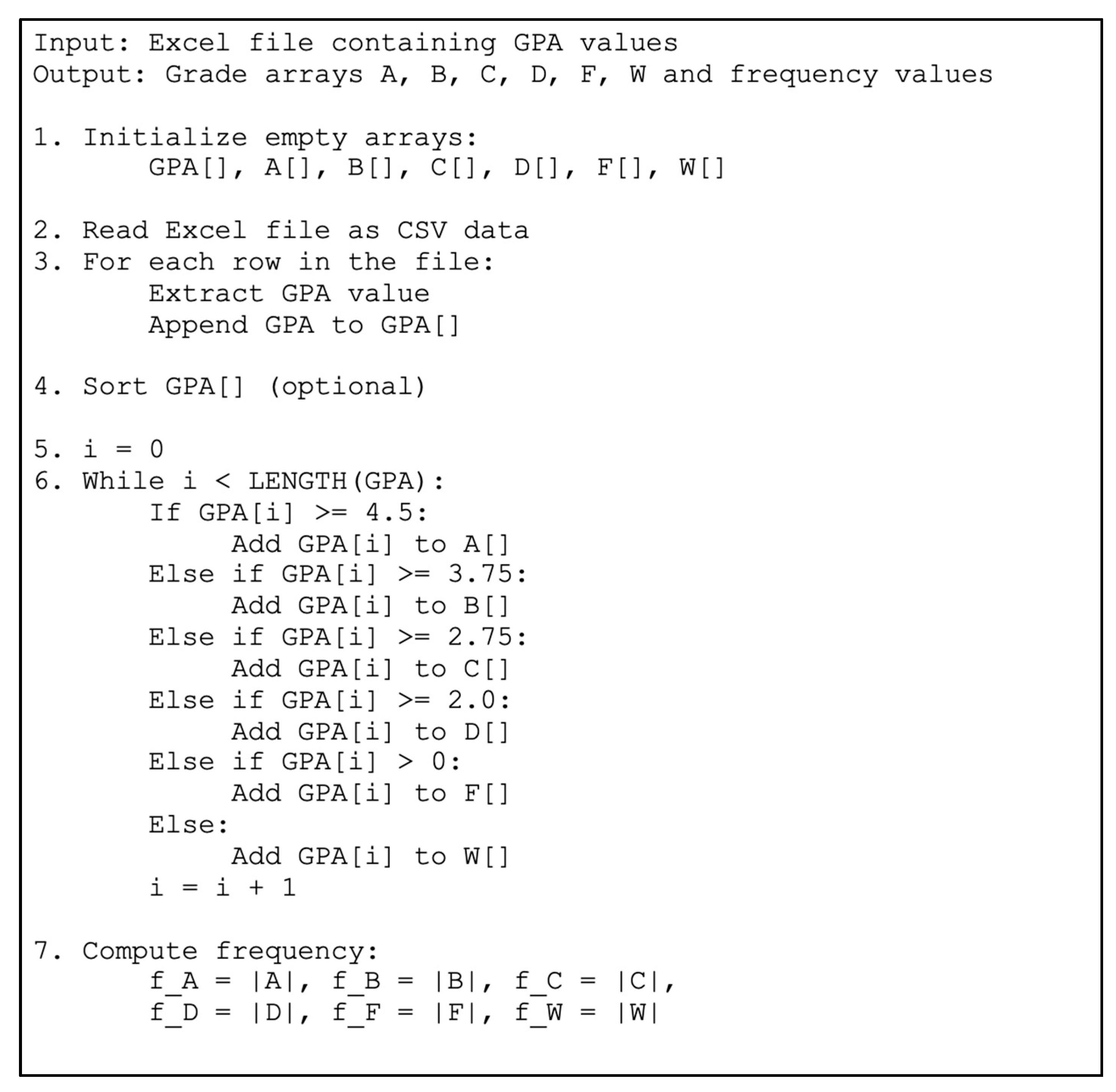
Figure 2.
Processing Algorithm.
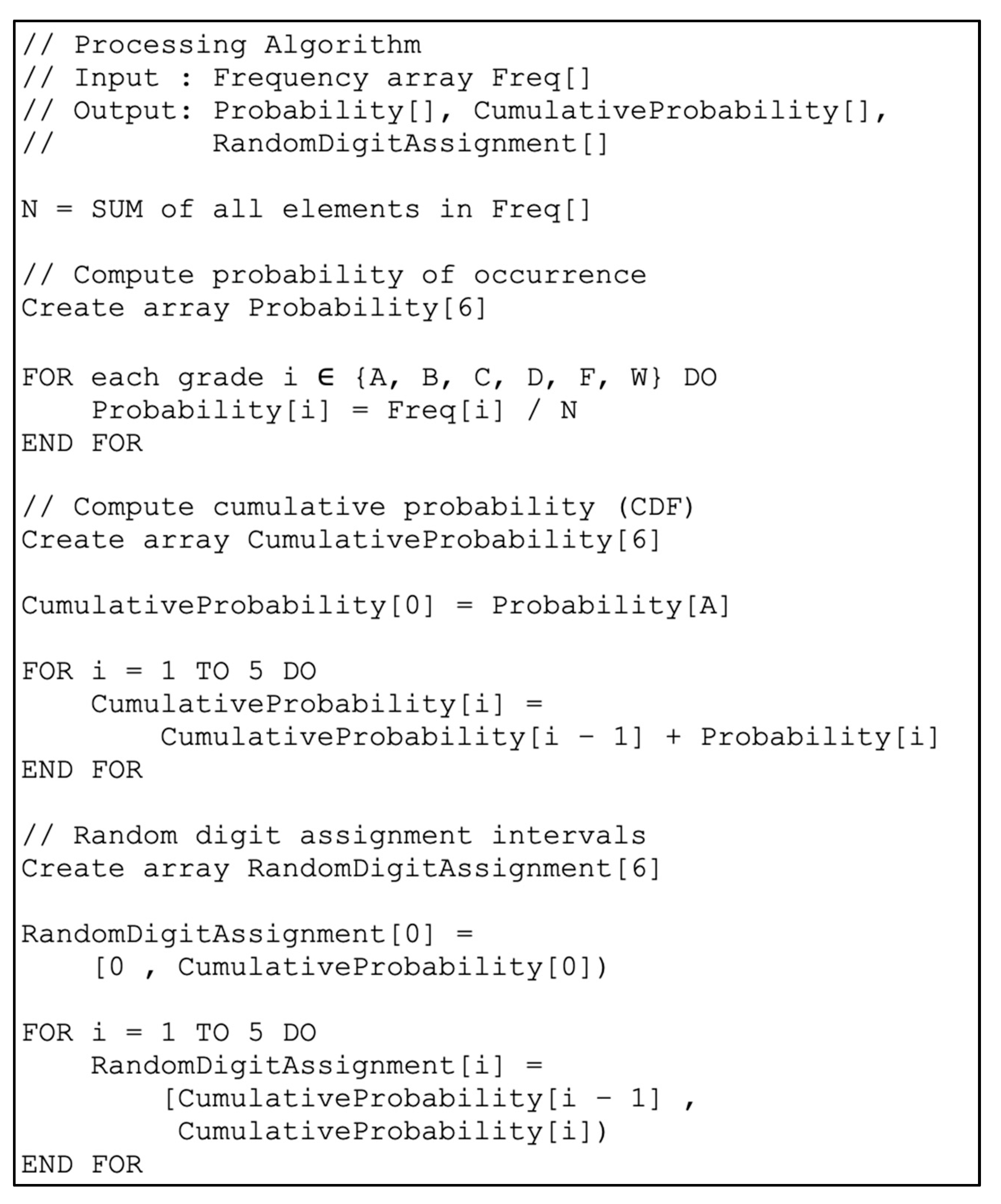
Figure 3.
Predicting Algorithm.
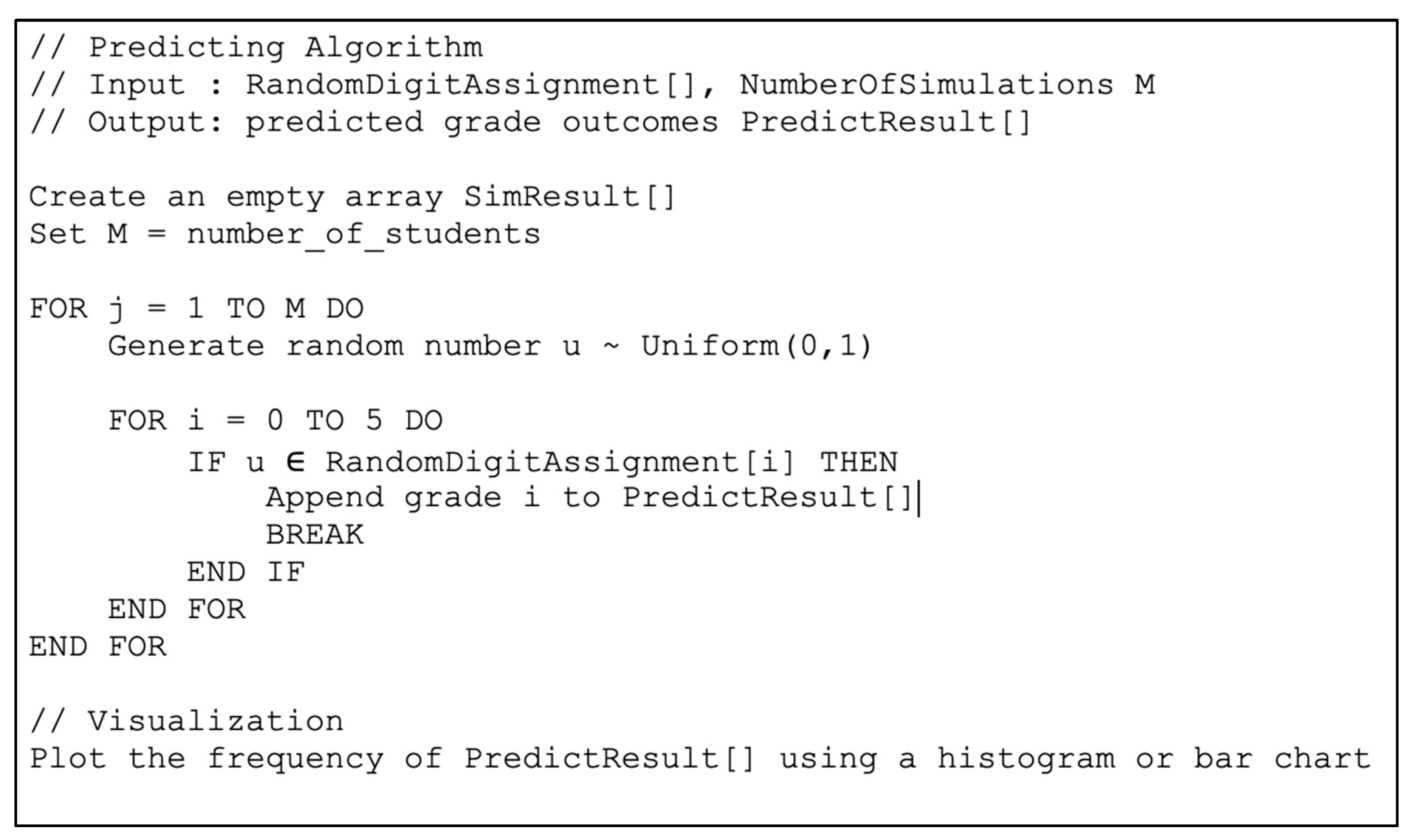
Figure 14.
Linear Regression Prediction Algorithm.
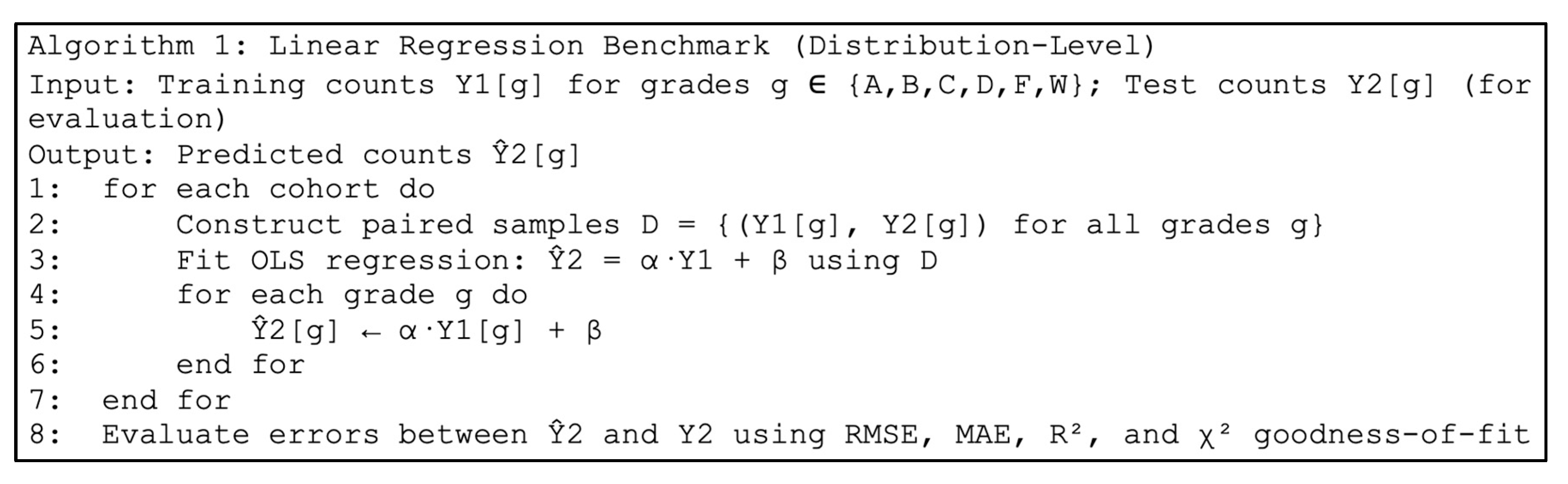
Figure 18.
Error summary (RMSE and MAE) for Regression vs Monte Carlo across cohorts.
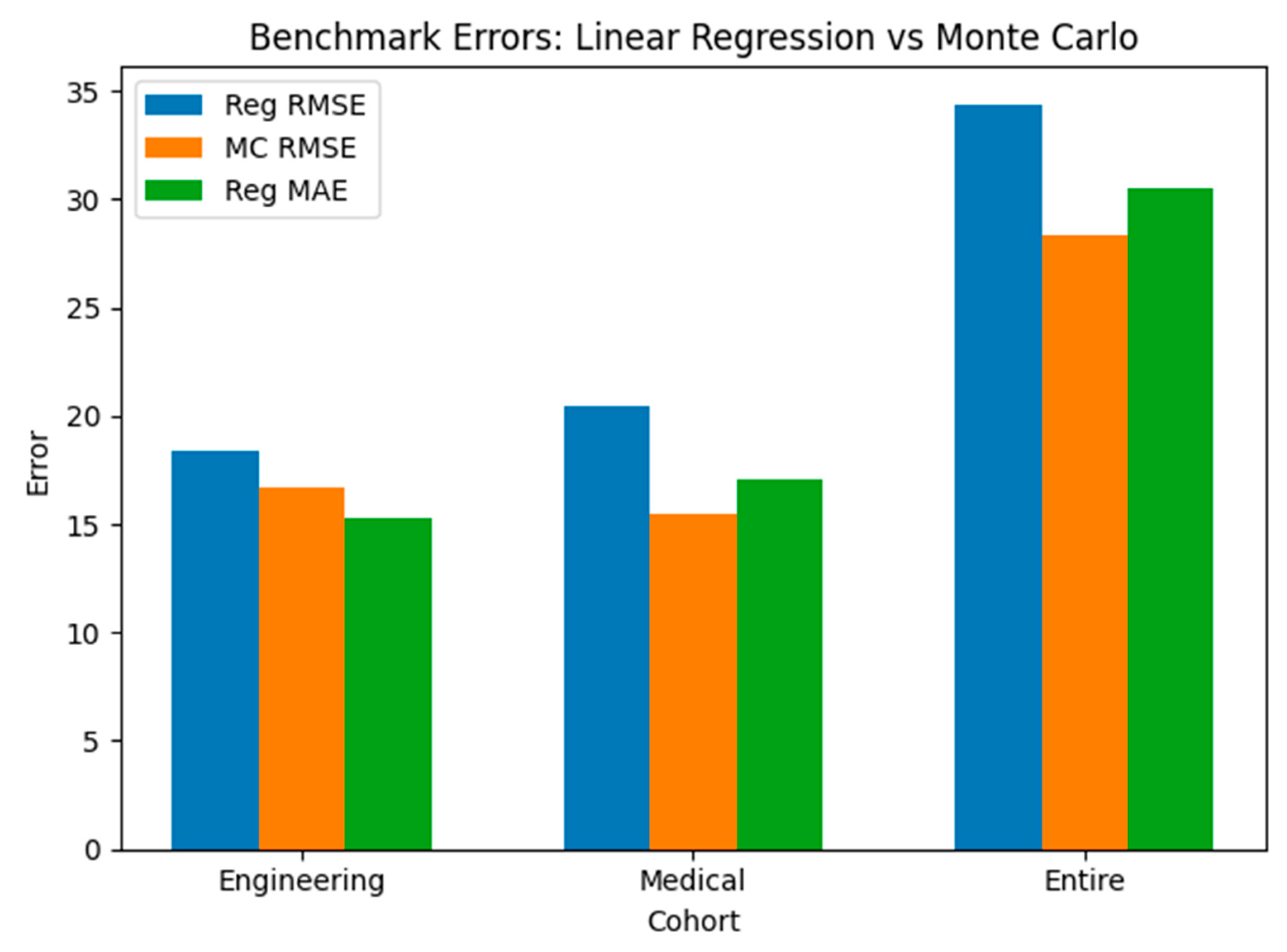
Figure 19.
Engineering Students: Residual comparison.
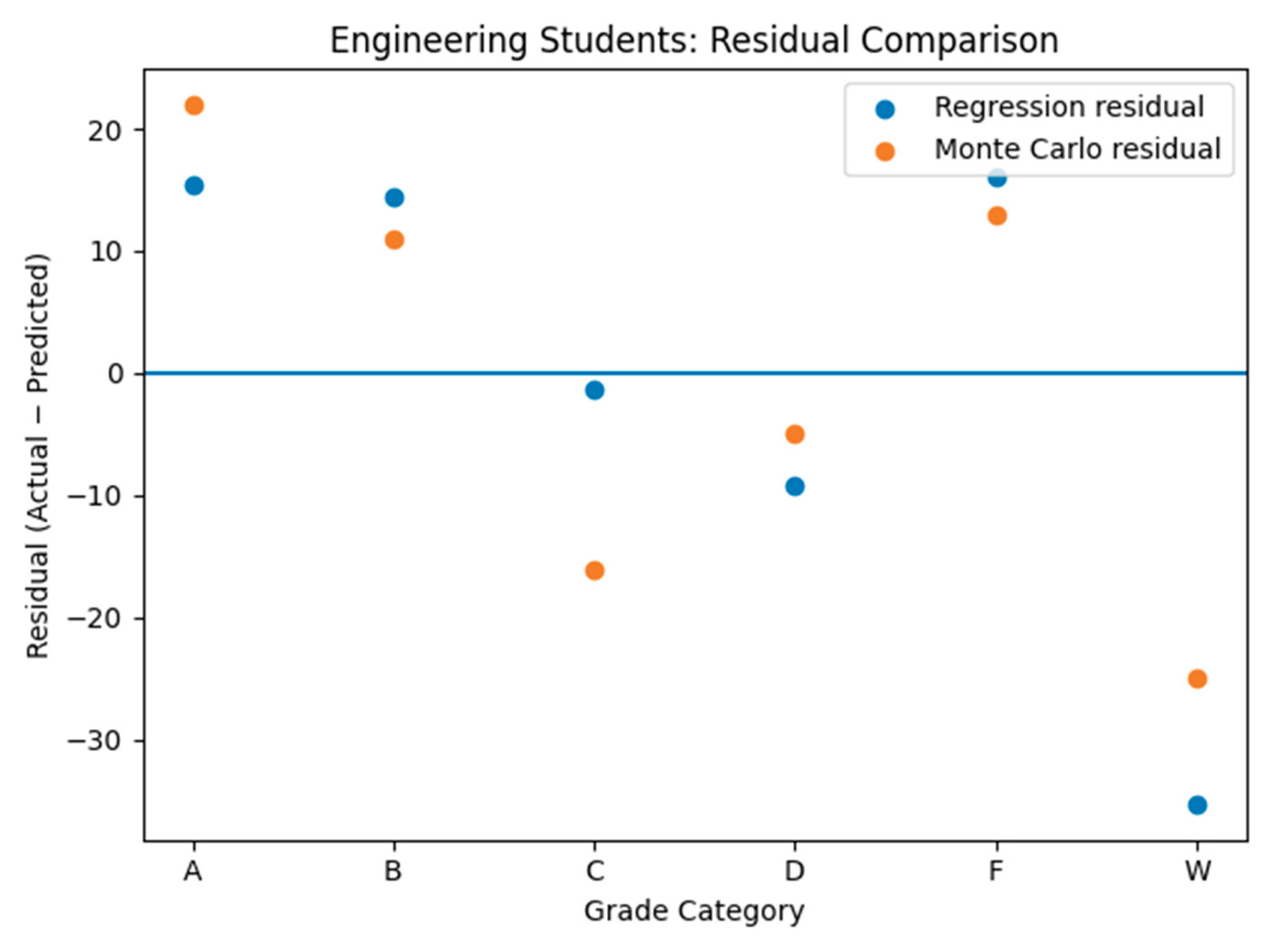
Figure 20.
Medical Students: Residual comparison.
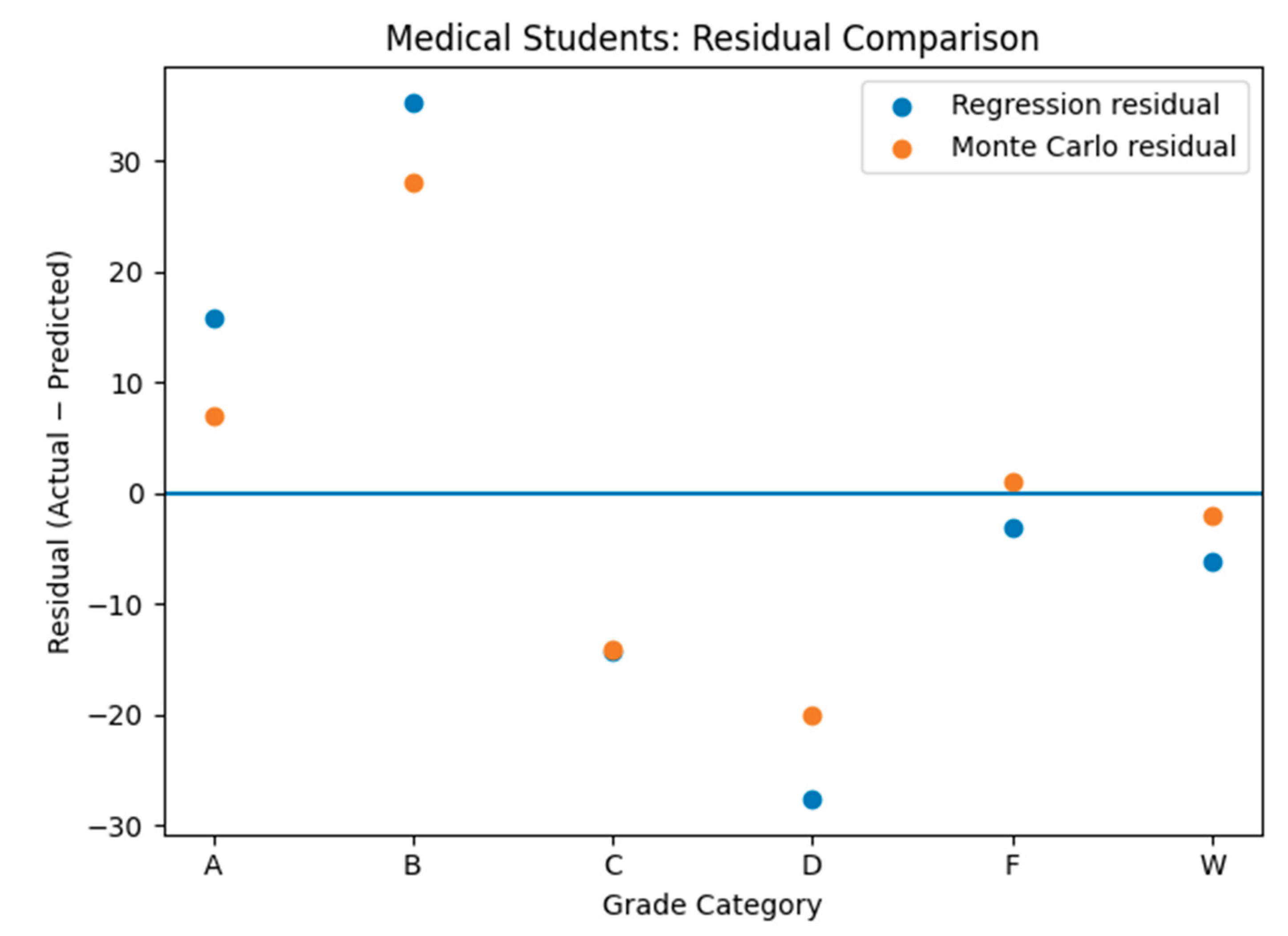
Figure 21.
Entire Students: Residual comparison.
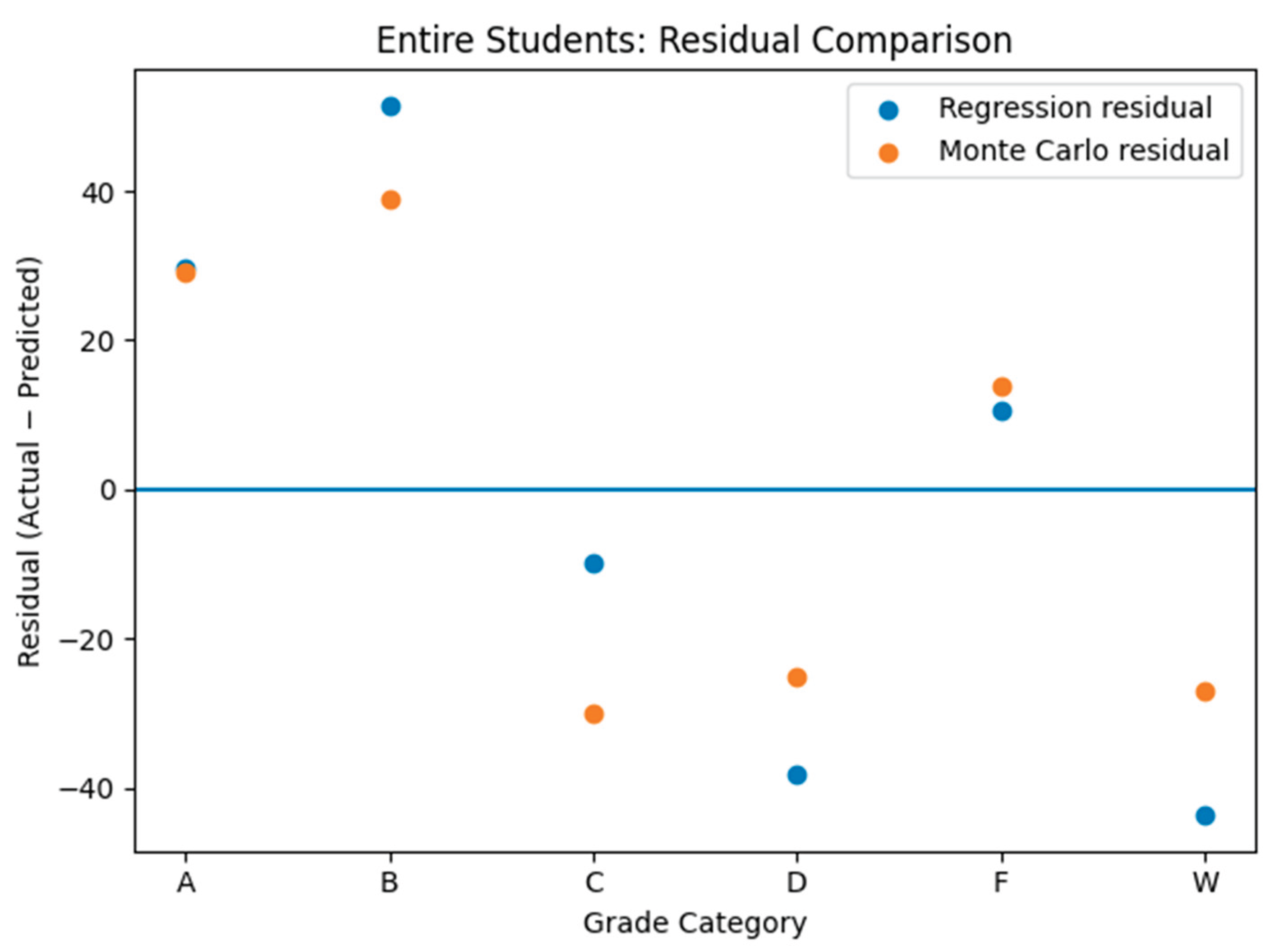

Table 1.
A sample of part of the original dataset for the year 2015/2016 () after de-identifying the data to protect student privacy.
Table 1.
A sample of part of the original dataset for the year 2015/2016 () after de-identifying the data to protect student privacy.
| # | High School Final Grade | Achievement Test Score | Aptitude Test Score | Weighted Admission Score | GPA |
|---|---|---|---|---|---|
| 28 | 81.5 | 74 | 84 | 79.2 | 2.56 |
| 29 | 91.3 | 65 | 67 | 73.5 | 2.95 |
| 30 | 91 | 64 | 74 | 75.1 | 2.54 |
| 31 | 91.2 | 70 | 72 | 77 | 3.31 |
| 32 | 96 | 71 | 88 | 83.6 | 2.42 |
| 33 | 84.6 | 69 | 80 | 77 | 2.71 |
| 34 | 90.7 | 65 | 80 | 77.2 | 3.08 |
| 35 | 91 | 69 | 74 | 77.1 | 3.35 |
| 36 | 92.8 | 66 | 66 | 74 | 3.05 |
| 37 | 90.6 | 63 | 71 | 73.7 | 2.88 |
| 38 | 98.5 | 64 | 66 | 74.9 | 3.52 |
| 39 | 95.3 | 65 | 68 | 75 | 2.18 |
| 40 | 82.9 | 67 | 70 | 72.7 | 2.81 |
| 41 | 79.4 | 64 | 79 | 73.1 | 2.18 |
| 42 | 91.8 | 67 | 66 | 74.2 | 3.15 |
| 43 | 89.1 | 64 | 79 | 76 | 2.91 |
Table 2.
The preprocessed result for the first year 2015/2016 () (the training dataset).
| Grade | Fequency | Grade | Fequency | Grade | Fequency |
|---|---|---|---|---|---|
| A | 32 | A | 51 | A | 83 |
| B | 110 | B | 124 | B | 234 |
| C | 217 | C | 214 | C | 431 |
| D | 111 | D | 63 | D | 174 |
| F | 126 | F | 41 | F | 167 |
| W | 79 | W | 44 | W | 123 |
| Total | 675 | Total | 537 | Total | 1212 |
| (a) | (b) | (c) | |||
| (a) engineer students (b) medical students (c) the entire dataset | |||||
Table 3.
The preprocessed result for the second year 2016/2017 () (the tested dataset).
| Grade | Fequency | Grade | Fequency | Grade | Fequency |
|---|---|---|---|---|---|
| A | 56 | A | 57 | A | 113 |
| B | 106 | B | 128 | B | 234 |
| C | 160 | C | 142 | C | 302 |
| D | 83 | D | 22 | D | 105 |
| F | 118 | F | 31 | F | 149 |
| W | 36 | W | 30 | W | 66 |
| Total | 559 | Total | 410 | Total | 969 |
| (a) | (b) | (c) | |||
| (a) engineer students (b) medical students (c) the entire dataset | |||||
Table 4.
The processed engineering students' training dataset.
| Grade | Fequency | Probability of occurrence | CDF | Random digit assignment intervals | |
| i | j | ||||
| A | 32 | 0.04740741 | 0.04740741 | 0.000001 | 0.04740741 |
| B | 110 | 0.16296296 | 0.21037037 | 0.04750741 | 0.21037037 |
| C | 217 | 0.32148148 | 0.53185185 | 0.21047037 | 0.53185185 |
| D | 111 | 0.16444444 | 0.6962963 | 0.53195185 | 0.6962963 |
| F | 126 | 0.18666667 | 0.88296296 | 0.6963963 | 0.88296296 |
| W | 79 | 0.11703704 | 1 | 0.88306296 | 1 |
| Total | 675 | ||||
Table 5.
The processed medical students' training dataset.
| Grade | Fequency | Probability of occurrence | CDF | Random digit assignment intervals | |
|---|---|---|---|---|---|
| i | j | ||||
| A | 51 | 0.09497207 | 0.09497207 | 0.000001 | 0.09497207 |
| B | 124 | 0.23091248 | 0.32588454 | 0.09497307 | 0.32588454 |
| C | 214 | 0.39851024 | 0.72439479 | 0.2120403 | 0.72439479 |
| D | 63 | 0.11731844 | 0.84171322 | 0.5359209 | 0.84171322 |
| F | 41 | 0.07635009 | 0.91806331 | 0.70159254 | 0.91806331 |
| W | 44 | 0.08193669 | 1 | 0.88965224 | 1 |
| Total | 537 | ||||
Table 6.
The processed entire training dataset.
| Grade | Fequency | Probability of occurrence | CDF | random digit assignment intervals | |
|---|---|---|---|---|---|
| i | j | ||||
| A | 83 | 0.06848185 | 0.06848185 | 0.000001 | 0.06848185 |
| B | 234 | 0.19306931 | 0.26155116 | 0.06848285 | 0.26155116 |
| C | 431 | 0.35561056 | 0.61716172 | 0.26155216 | 0.61716172 |
| D | 174 | 0.14356436 | 0.76072607 | 0.61716272 | 0.76072607 |
| F | 167 | 0.13778878 | 0.89851485 | 0.76072707 | 0.89851485 |
| W | 123 | 0.10148515 | 1 | 0.89851585 | 1 |
| Total | 1212 | ||||
Table 7.
Samples of the predicted GPAs.
| Engineer Student | Medical Student | Entire Student (All) | |||
|---|---|---|---|---|---|
| Random number | Predicted Grade | Random number | Predicted Grade | Random number | Predicted Grade |
| 0.663869666 | D | 0.34980756 | C | 0.20401078 | B |
| 0.991836546 | W | 0.40043125 | C | 0.43034441 | C |
| 0.472615915 | C | 0.74508802 | D | 0.78475392 | F |
| 0.689645622 | D | 0.03956323 | A | 0.40606519 | C |
| 0.449429594 | C | 0.38096823 | C | 0.38229142 | C |
| 0.111095292 | B | 0.19988857 | B | 0.69459553 | D |
| 0.173446769 | B | 0.75362121 | D | 0.99747801 | W |
| 0.170033622 | B | 0.41675629 | C | 0.30520837 | C |
| 0.779386763 | F | 0.39198222 | C | 0.3145153 | C |
| 0.803434742 | F | 0.09070375 | A | 0.23809493 | B |
| 0.689641122 | D | 0.02044473 | A | 0.30425396 | C |
| 0.090741882 | B | 0.45010105 | C | 0.87491963 | F |
| 0.545111037 | D | 0.13010809 | B | 0.30863828 | C |
| 0.754401154 | F | 0.45237335 | C | 0.59572846 | C |
| 0.242951276 | C | 0.99104339 | W | 0.69913296 | D |
| 0.452577487 | C | 0.14010158 | B | 0.77354354 | F |
| 0.731431025 | F | 0.25724328 | B | 0.61242481 | C |
| 0.303958095 | C | 0.46367026 | C | 0.75159288 | D |
| 0.761787723 | F | 0.94653363 | W | 0.3917825 | C |
| 0.585204504 | D | 0.29490198 | B | 0.35869343 | C |
| 0.703735663 | F | 0.76571015 | D | 0.46425459 | C |
| 0.949060214 | W | 0.2554432 | B | 0.84344466 | F |
| 0.488104358 | C | 0.35378027 | C | 0.30449036 | C |
| 0.59396983 | D | 0.76058732 | D | 0.17042966 | B |
Table 8.
Predicted vs. actual grade frequencies (counts).
| Cohort | Grade frequencies | A | B | C | D | F | W | Total |
|---|---|---|---|---|---|---|---|---|
| Engineering Students | Predicted | 34 | 95 | 176 | 88 | 105 | 61 | 559 |
| Actual | 56 | 106 | 160 | 83 | 118 | 36 | 559 | |
| Medical Students | Predicted | 50 | 100 | 156 | 42 | 30 | 32 | 410 |
| Actual | 57 | 128 | 142 | 22 | 31 | 30 | 410 | |
| Entire Students | Predicted | 84 | 195 | 332 | 130 | 135 | 93 | 969 |
| Actual | 113 | 234 | 302 | 105 | 149 | 66 | 969 |
Table 9.
Distribution-level evaluation metrics (Monte Carlo vs. actual).
| Metric | Engineering Students | Medical Students | Entire Students |
|---|---|---|---|
| N | 559 | 410 | 969 |
| RMSE | 16.733 | 15.460 | 28.320 |
| MAE | 15.333 | 12.000 | 27.333 |
| Chi² | 29.103 | 19.759 | 34.621 |
| p-value | 2.213e-05 | 1.387e-03 | 1.791e-06 |
| KL Divergence | 0.025476 | 0.025778 | 0.017767 |
| JS Divergence | 0.006359 | 0.006708 | 0.004442 |
| Total Variation | 0.082290 | 0.087805 | 0.084623 |
| Bhattacharyya | 0.006409 | 0.006767 | 0.004458 |
Table 10.
Residuals by grade category (Actual − Predicted) and total absolute residual.
| Cohort | Sum [Residual] |
||||||
| Engineering Students | 22 | 11 | -16 | -5 | 13 | -25 | 92 |
| Medical Students | 7 | 28 | -14 | -20 | 1 | -2 | 72 |
| Entire Students | 29 | 39 | -30 | -25 | 14 | -27 | 164 |
Table 11.
Training (Y₁), test (Y₂), and model predictions (Regression and Monte Carlo).
| Cohort | Series | A | B | C | D | F | W | Total |
| Engineering Students |
Y1 (Train) | 32 | 110 | 217 | 111 | 126 | 79 | 675 |
| Y2 (Actual) | 56 | 106 | 160 | 83 | 118 | 36 | 559 | |
| Regression Pred | 40.64 | 91.54 | 161.35 | 92.19 | 101.97 | 71.31 | 559.00 | |
| Monte Carlo Pred | 34 | 95 | 176 | 88 | 105 | 61 | 559 | |
| Medical Students |
Y1 (Train) | 51 | 124 | 214 | 63 | 41 | 44 | 537 |
| Y2 (Actual) | 57 | 128 | 142 | 22 | 31 | 30 | 410 | |
| Regression Pred | 41.15 | 92.69 | 156.24 | 49.62 | 34.09 | 36.21 | 410.00 | |
| Monte Carlo Pred | 50 | 100 | 156 | 42 | 30 | 32 | 410 | |
| Entire Students |
Y1 (Train) | 83 | 234 | 431 | 174 | 167 | 123 | 1212 |
| Y2 (Actual) | 113 | 234 | 302 | 105 | 149 | 66 | 969 | |
| Regression Pred | 83.35 | 182.52 | 311.89 | 143.11 | 138.51 | 109.62 | 969.00 | |
| Monte Carlo Pred | 84 | 195 | 332 | 130 | 135 | 93 | 969 |
Table 12.
Comparative Performance.
| Metric | Engineering students | Medical Students | Entire Students | |||
| Linear Regression | Monte Carlo | Linear Regression | Monte Carlo | Linear Regression | Monte Carlo | |
| RMSE | 18.416 | 16.733 | 20.460 | 15.460 | 34.382 | 28.320 |
| MAE | 15.282 | 15.333 | 17.052 | 12.000 | 30.540 | 27.333 |
| R² | 0.797 | 0.832 | 0.822 | 0.898 | 0.822 | 0.879 |
| Chi² | 29.016 | 29.103 | 37.572 | 19.759 | 53.684 | 34.621 |
| p-value | 2.302e-05 | 2.213e-05 | 4.598e-07 | 1.387e-03 | 2.434e-10 | 1.791e-06 |
Table 13.
linear regression parameters.
| Parameter | Engineering | Medical | Entire |
|---|---|---|---|
| Slope | 0.652 | 0.706 | 0.657 |
| Intercept | 19.767 | 5.143 | 28.841 |
Table 14.
Residual comparison.
| Metric | Engineering students | Medical Students | Entire Students | |||
| Linear Regression | Monte Carlo | Linear Regression | Linear Regression | Monte Carlo | Linear Regression | |
| Residual_A | 15.36 | 22.00 | 15.85 | 7.00 | 29.65 | 29.00 |
| Residual_B | 14.46 | 11.00 | 35.31 | 28.00 | 51.48 | 39.00 |
| Residual_C | -1.35 | -16.00 | -14.24 | -14.00 | -9.89 | -30.00 |
| Residual_D | -9.19 | -5.00 | -27.62 | -20.00 | -38.11 | -25.00 |
| Residual_F | 16.03 | 13.00 | -3.09 | 1.00 | 10.49 | 14.00 |
| Residual_W | -35.31 | -25.00 | -6.21 | -2.00 | -43.62 | -27.00 |
| SumAbsResidual | 91.69 | 92.00 | 102.31 | 72.00 | 183.24 | 164.00 |
Disclaimer/Publisher’s Note: The statements, opinions and data contained in all publications are solely those of the individual author(s) and contributor(s) and not of MDPI and/or the editor(s). MDPI and/or the editor(s) disclaim responsibility for any injury to people or property resulting from any ideas, methods, instructions or products referred to in the content. |
© 2026 by the authors. Licensee MDPI, Basel, Switzerland. This article is an open access article distributed under the terms and conditions of the Creative Commons Attribution (CC BY) license (http://creativecommons.org/licenses/by/4.0/).
Copyright: This open access article is published under a Creative Commons CC BY 4.0 license, which permit the free download, distribution, and reuse, provided that the author and preprint are cited in any reuse.


