Submitted:
11 February 2026
Posted:
12 February 2026
You are already at the latest version
Abstract
Every company conducts evaluations to ensure the quality of its product and services. One useful tool is the control chart. Multivariate simultaneous control charts, such as Max-Mchart, Max-Half-Mchart, Max-MEWMA, and Max-MCUSUM, are used to monitor the mean and variability simultaneously. The Max-Half-Mchart is advantageous because it can detect both small and large shifts in the mean and covariance matrix. However, outliers can cause the chi-square cumulative distribution function to approach one, leading the inverse standard normal cumulative distribution toward infinity and triggering masking and swamping effects. To overcome this, robust estimators of the mean and covariance matrix are required. Fast-MCD and Det-MCD are fast robust estimators based on the C-step algorithm. The results of the outlier detection show that the robust Max-Half-Mchart based on Det-MCD performs best for a small number of outliers, while the robust Max-Half-Mchart based on Fast-MCD and Det-MCD performs best for a large number of outliers. In terms of process shift detection, both robust Max-Half-Mchart based on Fast-MCD and Det-MCD can detect shifts effectively. Applications to OPC cement quality data and synthetic data indicate that the robust Max-Half-Mchart based on Det-MCD is the most sensitive to outliers.
Keywords:
Det-MCD
; simultaneous control chart
; fast-MCD
; multivariate
; OPC cement
1. Introduction
Cement companies are enterprises that primarily emphasize the production of high-quality cement [1]. Quality is closely associated with customer expectations. Product criteria are continually evolving, making quality a dynamic aspect. A product might be considered high quality at one point, but at another time, it may no longer meet the quality standards [2,3]. Statistical Process Control (SPC) comprises a collection of problem-solving tools that are helpful in achieving process stability and enhancing capabilities by reducing variability [4]. Control charts are a commonly employed method for quality monitoring [5].
Simultaneous control charts are utilized to monitor both the moving average and variability concurrently. The Max-MEWMA chart was introduced by Xie [6]. This chart was also investigated by Syahputra et al. [7], who applied it to steel products. Cheng and Thaga [5] introduced the Max-MCUSUM chart [8,9,10]. The Max-Mchart was initially proposed by Thaga and Gabaitiri [11], and their research demonstrated its ability to detect both small and large shifts in the process swiftly. Kruba et al. introduced the Max-Half-Mchart for individual observations [12,13,14] and subgroup observations [15]. The advantage of these control charts is their capability to detect out-of-control conditions when either small or large shifts occur in the mean and covariance matrix. Upon comparing the results, the Max-Half-Mchart consistently outperforms the Max-Mchart. Kruba et al. also proposed a Max-Mchart using bootstrap control limits [16].
Outlier data can lead to masking and swamping effects. The masking effect refers to cases of false negatives, which occur when several outliers are not identified even though the outliers are truly present [17]. Conversely, the swamping effect refers to cases of false positives, where non-outlier data are incorrectly classified as outliers [18]. In the Max-Half-Mchart, the presence of outliers may cause the cumulative distribution function of the chi-square distribution to approach one, resulting in the inverse of the standard normal cumulative distribution approaching infinity. Therefore, robust estimators are required to accurately estimate the process mean vector and covariance matrix [19]. Several robust estimators have been developed, including the Minimum Volume Ellipsoid (MVE) estimator introduced by Rousseeuw, which has a high breakdown point [20]. The Minimum Covariance Determinant (MCD) estimator, also introduced by Rousseeuw in 1984 [21], estimates the covariance matrix by selecting the subset with the smallest determinant among all possible subsets [22]. To improve computational efficiency, Rousseeuw and Driessen introduced a faster version known as the Fast Minimum Covariance Determinant (Fast-MCD) algorithm [23], which is now widely used as a robust estimator. Williems et al. proposed the Reweighted Minimum Covariance Determinant (RMCD) method [24], which improves efficiency through reweighting. Furthermore, Hubert et al. introduced the Deterministic Minimum Covariance Determinant (Det-MCD) method that utilizes six initial estimates [25].
Research on robust estimators has been conducted by Mashuri et al. [26], who applied a PCA-based Hotelling’s method integrated with the Fast-MCD algorithm. Their results showed higher accuracy than conventional methods. Ahsan et al. [27] proposed a robust and adaptive Hotelling’s control chart, which outperformed classical approaches in detecting outliers. Alfaro and Ortega [28] compared several robust Hotelling’s estimators and concluded that robust estimators perform better when data contain outliers.
Based on these findings, this study focuses on developing a robust Max-Half-Mchart control chart based on the Fast-MCD estimator and a robust Max-Half-Mchart control chart based on the Det-MCD estimator. These two robust control charts are then compared with the standard Max-Half-Mchart. All three control charts are applied to monitor the quality of Ordinary Portland Cement (OPC).
2. Material and Methods
2.1. Half-Normal Distribution
The half-normal distribution is derived from the normal distribution, where the random variable is defined as the absolute value of a normally distributed variable. This distribution is commonly used when sampling from a standard normal population in situations where negative observations are not admissible. Let follow a normal distribution with mean and standard deviation . Then, follows a half-normal distribution with parameters and . The probability density function (PDF) of a half-normal distribution with parameters and is given as follows:
When and , follows a standard half-normal distribution. The PDF of a standard half-normal random variable can be expressed as follows:
Let . The cumulative distribution function (CDF) of the standard half-normal distribution can then be written as follows:
where denotes the error function.
2.2. Maximum Half-Normal Multivariat Control Chart (Max-Half-Mchart)
Due to the inaccurate results produced by the Max-Mchart, an alternative approach is required. The half-normal transformation offers an appropriate solution because it yields strictly positive values, allowing it to overcome the limitations of the original Max-Mchart. The individual Max-Half-Mchart statistic is defined as follows [12]:
where
and
denotes the cumulative distribution function of the standard half-normal distribution, and represents the cumulative distribution function of the chi-square distribution with degrees of freedom. Since , the Max-Half-Mchart requires only an upper control limit (UCL). The UCL is determined using a bootstrap procedure [12].
Process shifts are identified by comparing the statistics with the UCL. When , an signal is generated, indicating a shift in the process mean. When , a signal is detected, reflecting a shift in process variability. If both and , a signal occurs, indicating simultaneous shifts in the process mean and variability.
2.3. Fast Minimum Covariance Determinant (Fast-MCD)
The Fast-MCD algorithm proposed by [23] provides a computationally efficient alternative to the classical MCD by using the Concentration Step (C-step). The algorithm proceeds as follows:
- a.
- Set .
- b.
- Obtain the estimates of and from the Phase I (in-control) data.
- c.
- Compute the Mahalanobis distances:
- d.
- Sort the distances in ascending order.
- e.
- Form a new subset consisting of the observations with the smallest distances.
- f.
- Compute from .
- g.
- Compare with Repeat the C-step until . The final subset is denoted with mean and covariance matrix .
The reweighted Fast-MCD estimators are:
with weights:
2.4. Deterministic Minimum Covariance Determinant (Det-MCD)
In the Det-MCD approach, each variable is first standardized by subtracting the median and dividing by the scale estimator as proposed by [30]. The estimator is defined as
where is a constant factor and , with . The value is used, and is obtained from the -th order statistic of the pairwise distances. The standardized data are denoted by the matrix , with rows and columns .
Six initial estimates of the center and scatter are then constructed. These initial scatter estimators are obtained as follows [25]:
- Compute for and define .
- Let be the ranks of and set , corresponding to the Spearman correlation.
- Compute , where is the standard normal CDF, and define .
- The fourth estimator is based on the spatial sign covariance matrix [31]. Define for all . Then,
- The fifth estimator uses the first step of the BACON algorithm [32], selecting the standardized observations with the smallest norms and computing their mean and covariance.
- The sixth estimator is the unweighted OGK estimator using the median and for and , respectively [33].
After obtaining , the following steps are performed:
- Compute the eigenvector matrix of and define .
- Calculate where
- Estimate the center of using
For each estimator , compute the statistical distance
Select the observations with the smallest values and compute the corresponding distance . Among the six initial estimators, choose the observations with the smallest values and apply the C-step until convergence. The resulting solution with the smallest determinant is referred to as the raw Det-MCD. The vectors and represent the center and covariance matrix of this solution.
Finally, apply the reweighting step:
where the weights are defined as
2.5. Proposed Robust Max-Half-Mchart Based on FMCD and Det-MCD
The implementation of the robust Max-Half-Mchart based on the Fast-MCD estimator is carried out by estimating the mean vector and covariance matrix using the Fast-MCD algorithm. Let denote the -variate observations. The vectors and represent the mean and covariance matrix obtained from the subset satisfying the condition in the Fast-MCD procedure. The robust Max-Half-M chart statistic based on the Fast-MCD estimator is defined as follows:
with
and
The robust Max-Half-M chart based on the Det-MCD estimator is constructed by estimating the mean vector and covariance matrix using the Det-MCD algorithm. Let denote the -variate observations. The vector and the matrix represent the mean and covariance matrix corresponding to the minimum-determinant solution obtained from the Det-MCD algorithm. These estimators are subsequently used in the construction of the robust Max-Half-M control chart. The corresponding robust Max-Half-M chart statistic based on the Det-MCD estimator is given as follows:
with
and
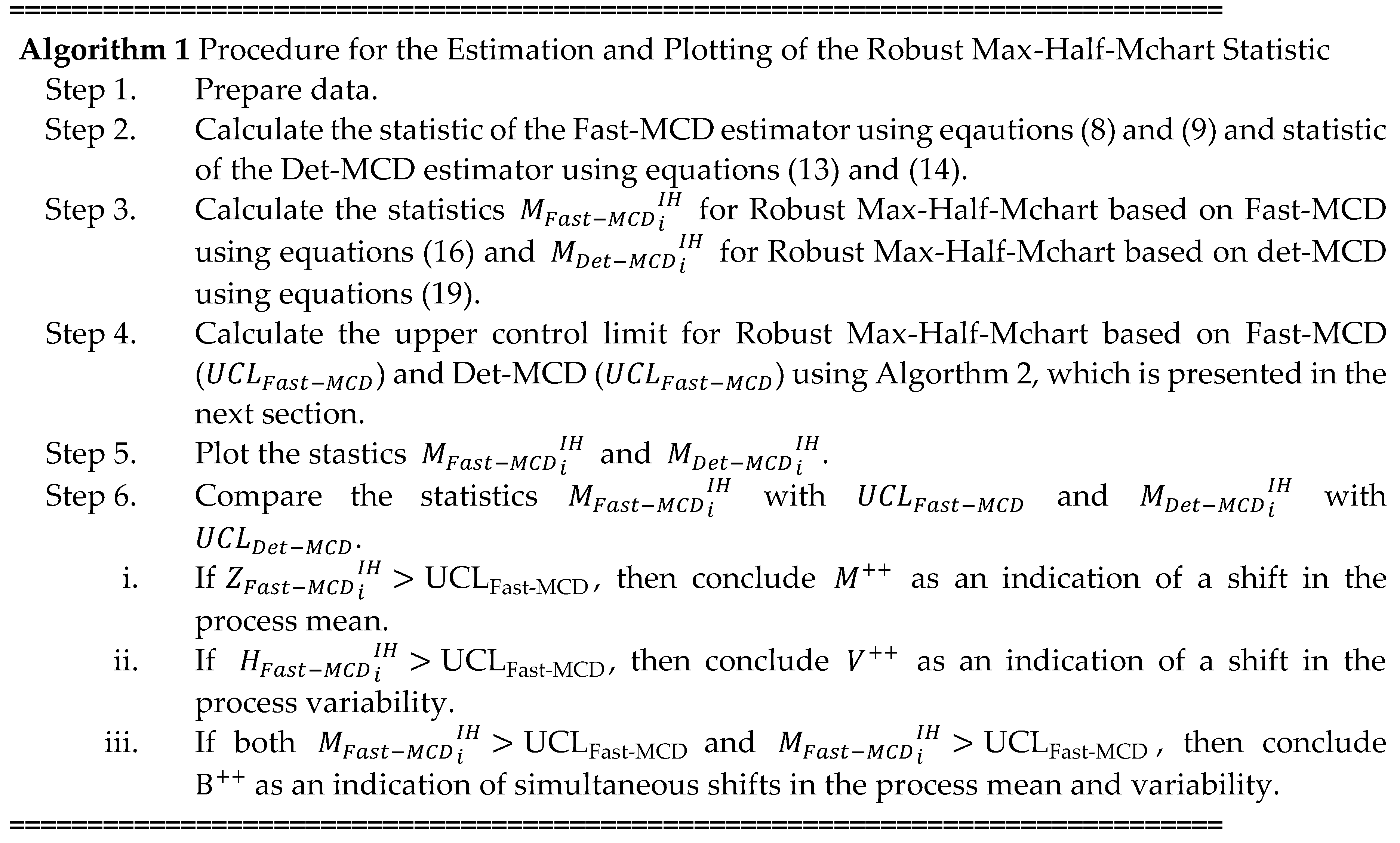
The steps for computing the statistics and constructing the robust Max-Half-M chart based on the Fast-MCD and Det-MCD estimator are given in Algorithm 1.
2.6. Control Limit of Proposed Robust Max-Half Mchart
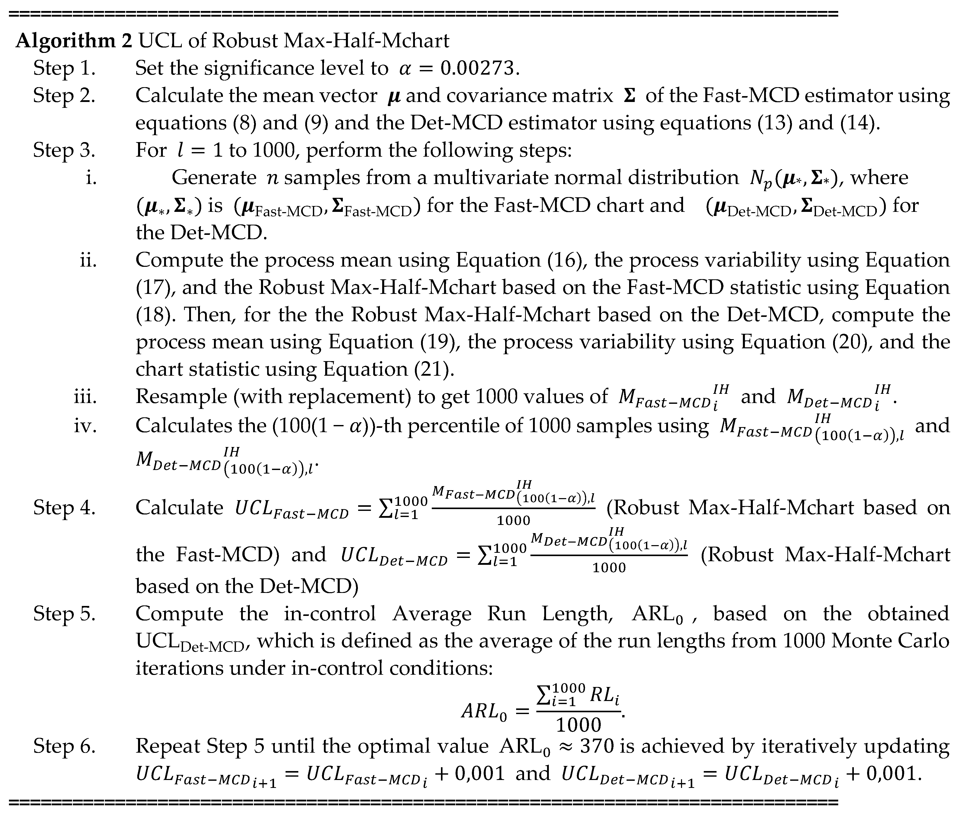
The robust Max-Half-M chart has only an upper control limit (UCL), since . However, because the Max-Half-M chart does not follow a specific known distribution. In this study, the performance of the Coventional Max-Half-Mchart and Robust Max-Half-Mchart based on the Fast-MCD and Det-MCD estimators is compared. To ensure a fair comparison between the conventional Max-Half-Mchart and the proposed Max-Half-M chart, both the bootstrap method and Monte Carlo simulation are employed to estimate their UCL values. The procedure for determining upper control limit (UCL) of the Max-Half-M chart using these approaches, is presented in Algorithm 2 as follows:
2.7. Method for Evaluating Perfomance of Proposed Robust Max-Half-Mchart
A control chart is considered effective when it is able to detect process shifts promptly. The faster a shift is detected, the better the performance of the control chart. Its detection capability is commonly evaluated using the Average Run Length (ARL). The ARL represents the average number of plotted points required before a point indicates an out-of-control condition [4]. There are two types of ARL that must be considered, namely and . The is defined as the expected average number of observations until the first point exceeds the control limits while the process is still in control [34]. The is given by
where denotes the Type I error, i.e., the probability of issuing an out-of-control signal when the process is actually in control. A commonly used value of for three-sigma (3σ) control limits is .
Meanwhile, denotes the expected average number of observations required to detect an out-of-control signal when the process is truly out of control. Thus, is defined as [24]
where represents the Type II error, i.e., the probability of failing to detect an out-of-control signal when a process shift has occurred. A control chart is considered to have good performance when it yields a sufficiently large and a sufficiently small .
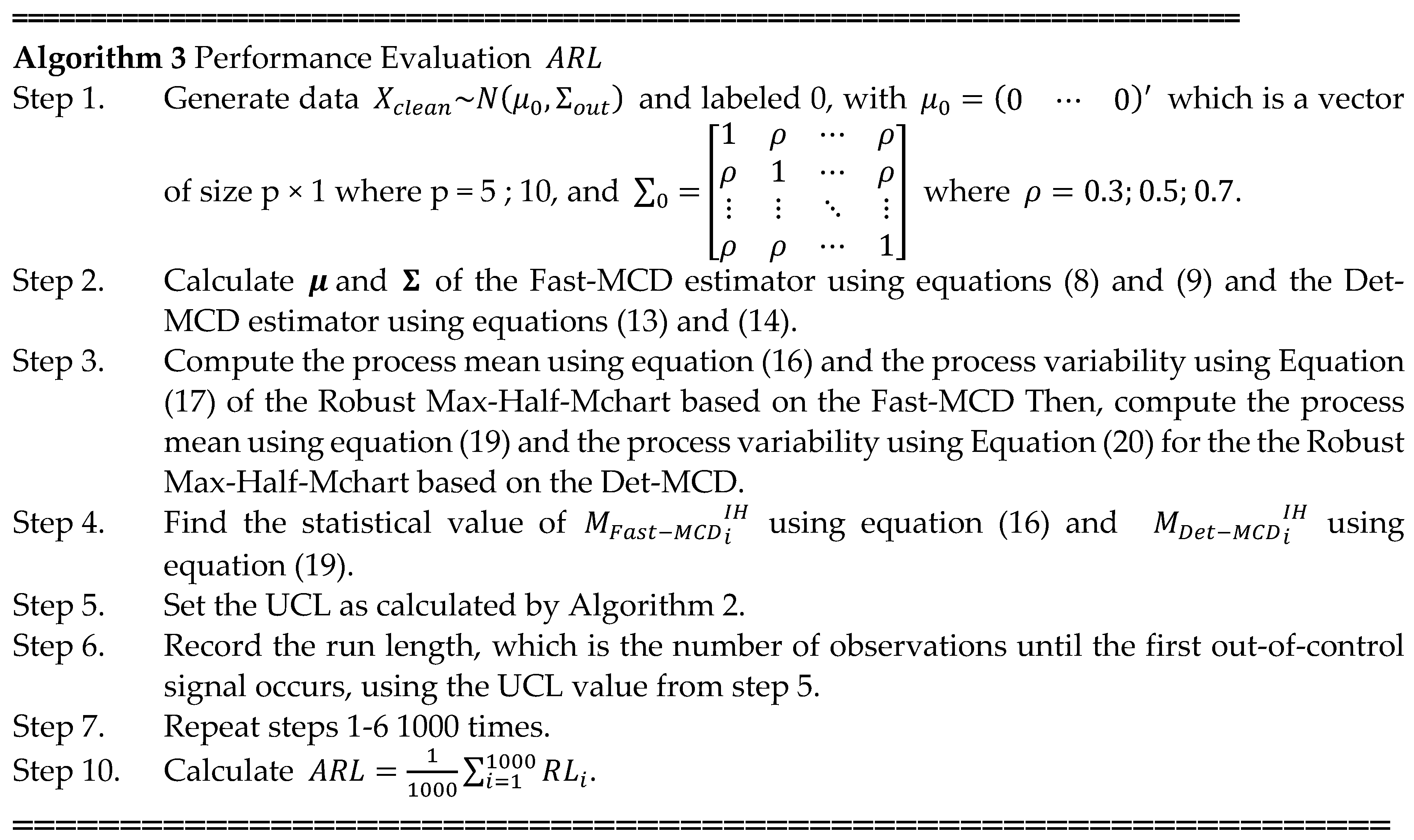
The step evaluation of the Robust Max-Half-Mchart for detecting process shifts is carried out based on the Average Run Length (ARL) criterion in Algorithm 3, as follows.
The performance of a control chart can also be evaluated based on classification accuracy. When outliers are correctly identified by the control chart, it indicates that the monitoring system operates properly and is able to provide relevant information about the process condition. Classification accuracy is evaluated through two main outcomes, namely True Positive (TP) and True Negative (TN). True Positive (TP) occurs when the control chart correctly detects the presence of an outlier and an outlier indeed exists. True Negative (TN) occurs when the control chart correctly identifies the absence of an outlier and no outlier actually exists.
In addition to TP and TN, other performance measures are also considered in evaluating detection systems, including False Positive (FP), which occurs when the control chart detects an outlier while no outlier is actually present, and False Negative (FN), which occurs when the control chart fails to detect an outlier even though an outlier is present. These four measures are jointly used to assess the reliability and accuracy of a monitoring system based on control charts.
The performance metrics used in this study include accuracy, false positive (FP) rate, false negative (FN) rate, and the area under the curve (AUC). Accuracy represents the proportion of correctly classified observations relative to the total number of observations and is defined as
There are two types of classification errors, namely the FP rate and the FN rate [27]. The FP rate is calculated as
Meanwhile, the FN rate is calculated as
The Area Under the Curve (AUC) is a measure of the area under the Receiver Operating Characteristic (ROC) curve. A higher AUC value indicates better classification performance. The AUC is computed as follows [35]:
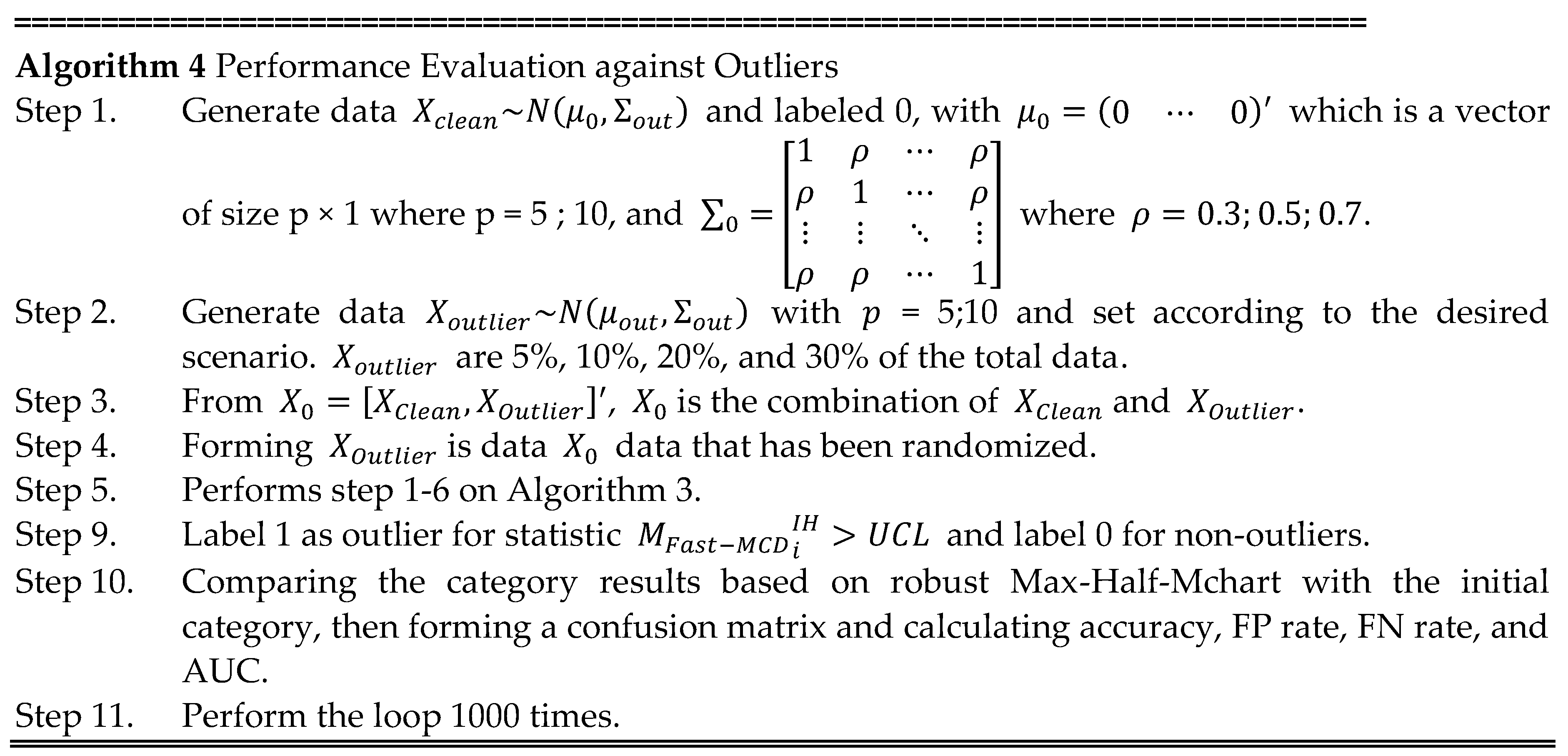
The step evaluation of the Robust Max-Half-Mchart for detecting outliers are calculated using Algorithm 4 as follows:
3. Results
3.1. Performance Robust Max-Half-Mchart in Process Shift
The performance of a control chart can be assessed based on its ability to promptly detect process shifts. One of the most widely used criteria for evaluating this detection capability is the Average Run Length (ARL). The ARL represents the average number of observations required before the control chart signals an out-of-control condition for the first time. A well-performing control chart is expected to exhibit a large , indicating a low false alarm rate under in-control conditions, and a small , reflecting rapid detection of actual process shifts. This balance ensures both reliability and responsiveness in process monitoring.
In this study, the ARL values were obtained through a simulation procedure following the steps presented in Algorithm 1, by considering various scenarios of shifts in the process mean, covariance matrix, and both of them with dimension quality characteristics and three correlation levels and . Through this approach, the performance of each control chart, the conventional Max-Half-Mchart and the robust versions based on Fast-MCD and Det-MCD, can be compared objectively and comprehensively in terms of their ability to detect process shifts.
Table 1 reports the ARL values for the three charts, namely the conventional Max-Half -chart and the robust Max-Half-Mcharts based on Fast-MCD and Det-MCD. When the mean vector shifts from to and the covariance matrix remains in-control (), the ARL of the conventional Max-Half -chart decreases from 373 to 310. The ARL further decreases from 372 to 80 when the covariance matrix is inflated by a factor of 1.5 () while the mean vector remains in-control (). For the robust Max-Half-Mchart based on Fast-MCD, the ARL decreases from 371 to 326 when the mean vector shifts, and from 371 to 80 when the covariance matrix is inflated by a factor of 1.5 () with the mean vector still in-control. Similarly, the ARL of the robust Max-Half-Mchart based on Det-MCD decreases from 371 to 311 under a mean shift, and from 371 to 73 when the covariance matrix is inflated by a factor of 1.5 () while the mean vector remains in-control. These findings indicate that the robust Max- Max-Half-Mchart based on Det-MCD detects changes in the covariance matrix more quickly than changes in the mean vector, and does so more efficiently than both the conventional Max-Half-Mchart and the robust Max-Half-Mchart based on Fast-MCD. In contrast, the conventional Max-Half-Mchart is relatively faster in detecting mean shifts than covariance shifts when compared with the robust Max-Half-Mchart based on Fast-MCD and Det-MCD.
The conventional Max-Half-Mchart based is also slightly more sensitive for individual observations in detecting large shifts. This is evident when the mean vector shifts from to while the covariance matrix is in-control (), where the ARL decreases from 373 to 1. Meanwhile, the ARL decreases from 373 to 2 when the covariance matrix is inflated by a factor and the mean vector remains in-control. On the other hand, the ARL of the robust Max-Half-Mchart based on Det-MCD decreases from 371 to 1 when the mean vector shifts from to with the covariance matrix in-control (). Furthermore, the ARL decreases from 371 to approximately 1 when the covariance matrix is inflated by a factor and the mean vector remains in-control ().
Table 3 reports the ARL values of the conventional Max-Half- for . The ARL decreases from 372 to 4 when the mean vector shifts from to , while the covariance matrix remains in-control . When the covariance matrix is inflated by a factor of 4 and the mean vector remains in-control , ARL decreases from 372 to approximately 2.
Table 3 also summarizes the ARL values of the robust Max-Half-Mchart based on Fast-MCD for . In this case, the ARL decreases from 370 to 3 when the mean vector shifts from to and the covariance matrix is in-control . When the covariance matrix is inflated by a factor of 4 and the mean vector remains in-control , ARL decreases from 370 to approximately 2.
Similarly, the ARL of the robust Max-Half-Mchart based on Det-MCD decreases from 371 to 3 when the mean vector shifts from to with the covariance matrix in-control . When the covariance matrix is inflated by a factor of 4 and the mean vector remains in-control , ARL decreases from 371 to approximately 2. The results suggest that the correlation structure has a substantial impact on the performance of the robust Max-Half-Mchart based on Det-MCD in detecting shifts in both the mean vector and the covariance matrix. By comparing the findings in Table 1, Table 2 and Table 3, it can be concluded that the robust Det-MCD-based Max-Half -chart performs better for less correlated quality characteristics.

Table 2.
Performance. ARL Simulation with Correlation Levels
| a | b | ||||||||||||
| 1 | 1.25 | 1.5 | 1.75 | 2 | 2.25 | 2.5 | 2.75 | 3 | 3.25 | 3.5 | 3.75 | 4 | |
| 0 | 372.63 | 77.76 | 28.61 | 14.08 | 9.20 | 6.02 | 4.43 | 3.59 | 2.88 | 2.62 | 2.23 | 1.96 | 1.82 |
| 371.18 | 79.93 | 29.23 | 14.64 | 9.03 | 5.95 | 4.48 | 3.72 | 3.14 | 2.59 | 2.33 | 2.02 | 1.89 | |
| 371.84 | 79.89 | 29.86 | 14.59 | 9.07 | 6.15 | 4.76 | 3.51 | 2.99 | 2.60 | 2.38 | 2.03 | 1.88 | |
| 0.25 | 310.73 | 69.61 | 26.54 | 13.54 | 8.22 | 6.28 | 4.54 | 3.37 | 2.90 | 2.46 | 2.25 | 1.96 | 1.80 |
| 327.88 | 77.68 | 28.58 | 13.94 | 8.87 | 5.79 | 4.32 | 3.64 | 2.87 | 2.57 | 2.29 | 2.01 | 1.84 | |
| 327.81 | 76.16 | 26.86 | 14.64 | 9.41 | 6.44 | 4.33 | 3.50 | 2.94 | 2.52 | 2.23 | 1.98 | 1.88 | |
| 0.5 | 250.25 | 61.66 | 23.74 | 12.82 | 7.57 | 5.70 | 4.10 | 3.25 | 2.78 | 2.40 | 2.10 | 1.96 | 1.77 |
| 269.19 | 60.37 | 24.77 | 12.62 | 8.33 | 5.86 | 4.26 | 3.54 | 2.92 | 2.55 | 2.19 | 2.03 | 1.82 | |
| 245.23 | 64.06 | 25.26 | 13.34 | 7.85 | 5.87 | 4.21 | 3.50 | 2.89 | 2.56 | 2.21 | 1.96 | 1.88 | |
| 0.75 | 158.08 | 43.85 | 19.55 | 11.10 | 7.11 | 4.92 | 3.83 | 3.29 | 2.73 | 2.28 | 2.04 | 1.92 | 1.80 |
| 181.14 | 46.33 | 20.51 | 11.29 | 7.42 | 5.09 | 4.07 | 3.20 | 2.75 | 2.43 | 2.05 | 1.95 | 1.78 | |
| 177.03 | 49.12 | 20.15 | 11.04 | 7.44 | 5.20 | 4.12 | 3.39 | 2.84 | 2.40 | 2.10 | 1.96 | 1.78 | |
| 1 | 98.40 | 30.59 | 14.74 | 9.37 | 5.92 | 4.82 | 3.58 | 2.99 | 2.50 | 2.28 | 1.99 | 1.83 | 1.62 |
| 100.54 | 32.08 | 16.15 | 9.76 | 6.09 | 4.53 | 3.57 | 3.04 | 2.61 | 2.35 | 2.02 | 1.89 | 1.76 | |
| 101.83 | 33.90 | 16.09 | 9.45 | 6.17 | 4.63 | 3.69 | 3.11 | 2.69 | 2.17 | 2.06 | 1.90 | 1.78 | |
| 1.25 | 50.67 | 21.11 | 11.09 | 6.77 | 5.33 | 4.11 | 3.22 | 2.72 | 2.38 | 2.10 | 1.92 | 1.74 | 1.64 |
| 55.15 | 22.28 | 12.36 | 7.12 | 5.62 | 4.11 | 3.29 | 2.76 | 2.48 | 2.21 | 1.97 | 1.73 | 1.59 | |
| 54.99 | 22.49 | 11.43 | 7.24 | 5.17 | 4.27 | 3.49 | 2.85 | 2.47 | 2.11 | 1.88 | 1.72 | 1.61 | |
| 1.5 | 28.29 | 13.90 | 8.12 | 5.70 | 4.15 | 3.51 | 2.84 | 2.58 | 2.23 | 1.92 | 1.87 | 1.67 | 1.56 |
| 29.34 | 15.13 | 8.67 | 5.79 | 4.29 | 3.77 | 2.87 | 2.53 | 2.25 | 1.97 | 1.89 | 1.74 | 1.58 | |
| 29.02 | 13.87 | 8.62 | 5.92 | 4.59 | 3.52 | 2.92 | 2.41 | 2.26 | 1.98 | 1.84 | 1.72 | 1.60 | |
| 1.75 | 15.89 | 8.71 | 6.10 | 4.59 | 3.30 | 2.97 | 2.56 | 2.28 | 1.96 | 1.83 | 1.72 | 1.60 | 1.48 |
| 17.03 | 9.07 | 6.20 | 4.41 | 3.61 | 3.01 | 2.54 | 2.30 | 2.03 | 1.84 | 1.68 | 1.59 | 1.54 | |
| 17.08 | 9.18 | 6.53 | 4.63 | 3.45 | 2.95 | 2.53 | 2.27 | 2.00 | 1.88 | 1.68 | 1.60 | 1.57 | |
| 2 | 9.78 | 6.43 | 4.72 | 3.52 | 2.99 | 2.54 | 2.21 | 1.97 | 1.75 | 1.66 | 1.56 | 1.52 | 1.44 |
| 9.65 | 6.35 | 4.56 | 3.61 | 3.01 | 2.57 | 2.14 | 1.96 | 1.86 | 1.70 | 1.63 | 1.52 | 1.43 | |
| 10.15 | 5.89 | 4.43 | 3.61 | 3.04 | 2.59 | 2.24 | 2.04 | 1.86 | 1.71 | 1.56 | 1.52 | 1.46 | |
| 2.25 | 6.18 | 4.18 | 3.44 | 2.79 | 2.55 | 2.19 | 1.94 | 1.82 | 1.66 | 1.54 | 1.51 | 1.45 | 1.34 |
| 6.18 | 4.28 | 3.47 | 3.05 | 2.51 | 2.27 | 1.98 | 1.85 | 1.73 | 1.56 | 1.47 | 1.42 | 1.41 | |
| 6.07 | 4.46 | 3.39 | 2.95 | 2.45 | 2.23 | 1.98 | 1.81 | 1.67 | 1.60 | 1.55 | 1.41 | 1.38 | |
| 2.5 | 4.01 | 3.17 | 2.64 | 2.35 | 2.03 | 1.87 | 1.82 | 1.63 | 1.54 | 1.46 | 1.38 | 1.38 | 1.34 |
| 3.98 | 3.24 | 2.65 | 2.35 | 2.07 | 1.90 | 1.72 | 1.63 | 1.48 | 1.46 | 1.40 | 1.34 | 1.32 | |
| 4.13 | 3.08 | 2.74 | 2.32 | 2.25 | 1.91 | 1.80 | 1.63 | 1.60 | 1.48 | 1.45 | 1.36 | 1.29 | |
| 2.75 | 2.70 | 2.47 | 2.04 | 1.91 | 1.85 | 1.68 | 1.54 | 1.57 | 1.43 | 1.39 | 1.34 | 1.29 | 1.27 |
| 2.92 | 2.43 | 2.25 | 1.95 | 1.76 | 1.70 | 1.59 | 1.51 | 1.47 | 1.42 | 1.37 | 1.28 | 1.27 | |
| 3.08 | 2.54 | 2.10 | 1.99 | 1.80 | 1.76 | 1.59 | 1.55 | 1.40 | 1.37 | 1.36 | 1.28 | 1.28 | |
| 3 | 2.14 | 1.91 | 1.78 | 1.72 | 1.57 | 1.50 | 1.43 | 1.41 | 1.37 | 1.29 | 1.23 | 1.23 | 1.20 |
| 2.09 | 1.90 | 1.81 | 1.70 | 1.55 | 1.54 | 1.49 | 1.39 | 1.35 | 1.29 | 1.28 | 1.24 | 1.22 | |
| 2.19 | 1.93 | 1.80 | 1.67 | 1.60 | 1.46 | 1.41 | 1.37 | 1.34 | 1.31 | 1.25 | 1.26 | 1.21 | |
Table 3.
Performance. ARL Simulation with Correlation Levels
| a | b | ||||||||||||
| 1 | 1.25 | 1.5 | 1.75 | 2 | 2.25 | 2.5 | 2.75 | 3 | 3.25 | 3.5 | 3.75 | 4 | |
| 0 | 372.44 | 77.84 | 28.33 | 14.09 | 8.70 | 5.85 | 4.56 | 3.48 | 2.93 | 2.59 | 2.30 | 2.00 | 1.87 |
| 370.54 | 77.70 | 29.56 | 14.84 | 9.36 | 6.13 | 4.53 | 3.72 | 3.09 | 2.51 | 2.31 | 1.98 | 1.87 | |
| 371.37 | 78.65 | 27.79 | 14.82 | 8.82 | 6.07 | 4.85 | 3.63 | 3.06 | 2.48 | 2.21 | 2.09 | 1.90 | |
| 0.25 | 308.73 | 71.61 | 26.26 | 14.57 | 9.26 | 6.15 | 4.32 | 3.52 | 2.92 | 2.48 | 2.20 | 1.98 | 1.87 |
| 337.26 | 75.36 | 29.64 | 14.69 | 9.26 | 6.27 | 4.42 | 3.64 | 2.96 | 2.50 | 2.16 | 1.97 | 1.87 | |
| 312.42 | 74.74 | 28.28 | 14.01 | 8.37 | 6.06 | 4.63 | 3.48 | 3.04 | 2.48 | 2.21 | 2.02 | 1.85 | |
| 0.5 | 251.44 | 63.97 | 24.55 | 13.34 | 7.82 | 5.84 | 4.27 | 3.53 | 2.92 | 2.47 | 2.18 | 1.95 | 1.87 |
| 273.39 | 69.17 | 26.64 | 12.82 | 8.02 | 5.88 | 4.42 | 3.46 | 3.00 | 2.44 | 2.16 | 1.94 | 1.86 | |
| 282.69 | 66.05 | 25.86 | 14.14 | 8.39 | 5.68 | 4.30 | 3.48 | 2.98 | 2.46 | 2.18 | 1.97 | 1.85 | |
| 0.75 | 194.19 | 51.68 | 21.28 | 11.60 | 7.64 | 5.18 | 4.22 | 3.40 | 2.83 | 2.37 | 2.10 | 1.94 | 1.80 |
| 202.89 | 54.29 | 22.03 | 11.90 | 7.58 | 5.57 | 4.23 | 3.37 | 2.87 | 2.36 | 2.16 | 2.02 | 1.84 | |
| 203.59 | 53.51 | 22.96 | 12.65 | 7.63 | 5.38 | 3.98 | 3.35 | 2.75 | 2.44 | 2.15 | 1.90 | 1.88 | |
| 1 | 126.91 | 37.13 | 17.74 | 9.83 | 6.47 | 4.70 | 3.81 | 3.09 | 2.75 | 2.23 | 2.10 | 1.92 | 1.79 |
| 124.60 | 39.58 | 17.35 | 9.97 | 6.77 | 5.32 | 3.92 | 3.20 | 2.55 | 2.33 | 2.16 | 1.93 | 1.83 | |
| 124.92 | 38.23 | 18.24 | 10.37 | 6.87 | 5.06 | 3.97 | 3.22 | 2.63 | 2.40 | 2.11 | 1.92 | 1.69 | |
| 1.25 | 72.12 | 27.71 | 13.50 | 7.89 | 5.46 | 4.52 | 3.64 | 2.88 | 2.53 | 2.16 | 1.94 | 1.75 | 1.63 |
| 78.04 | 26.61 | 14.87 | 8.16 | 6.27 | 4.35 | 3.58 | 2.94 | 2.55 | 2.23 | 1.92 | 1.86 | 1.71 | |
| 77.60 | 27.39 | 13.57 | 8.18 | 6.10 | 4.17 | 3.42 | 2.83 | 2.62 | 2.14 | 1.98 | 1.80 | 1.69 | |
| 1.5 | 40.55 | 18.17 | 10.45 | 6.68 | 5.18 | 3.79 | 3.16 | 2.61 | 2.32 | 2.04 | 1.87 | 1.79 | 1.64 |
| 45.70 | 19.12 | 10.44 | 6.92 | 5.06 | 4.01 | 3.25 | 2.67 | 2.28 | 1.99 | 1.92 | 1.76 | 1.67 | |
| 44.03 | 20.05 | 10.34 | 6.96 | 5.31 | 3.92 | 3.32 | 2.71 | 2.25 | 2.14 | 1.96 | 1.69 | 1.64 | |
| 1.75 | 25.97 | 11.60 | 7.67 | 5.51 | 4.27 | 3.32 | 2.83 | 2.57 | 2.12 | 1.92 | 1.76 | 1.59 | 1.51 |
| 25.59 | 12.95 | 7.85 | 5.57 | 4.46 | 3.48 | 2.92 | 2.53 | 2.18 | 1.92 | 1.77 | 1.65 | 1.53 | |
| 27.01 | 13.66 | 7.71 | 5.60 | 4.04 | 3.27 | 2.78 | 2.37 | 2.02 | 1.94 | 1.81 | 1.67 | 1.56 | |
| 2 | 14.65 | 8.97 | 5.80 | 4.17 | 3.36 | 2.91 | 2.56 | 2.30 | 1.99 | 1.83 | 1.70 | 1.55 | 1.50 |
| 15.94 | 8.75 | 5.59 | 4.45 | 3.58 | 2.96 | 2.57 | 2.29 | 2.10 | 1.82 | 1.67 | 1.62 | 1.48 | |
| 10.15 | 5.89 | 4.43 | 3.61 | 3.04 | 2.59 | 2.24 | 2.04 | 1.86 | 1.71 | 1.56 | 1.52 | 1.46 | |
| 2.25 | 16.46 | 8.55 | 5.93 | 4.61 | 3.39 | 2.98 | 2.59 | 2.25 | 1.97 | 1.79 | 1.74 | 1.63 | 1.45 |
| 9.48 | 5.83 | 4.48 | 3.57 | 2.86 | 2.46 | 2.28 | 2.00 | 1.86 | 1.72 | 1.61 | 1.45 | 1.39 | |
| 9.96 | 6.14 | 4.67 | 3.71 | 3.02 | 2.61 | 2.21 | 2.07 | 1.83 | 1.81 | 1.62 | 1.54 | 1.46 | |
| 2.5 | 10.54 | 6.61 | 4.54 | 3.65 | 2.82 | 2.74 | 2.28 | 1.99 | 1.89 | 1.72 | 1.55 | 1.47 | 1.45 |
| 6.20 | 4.30 | 3.46 | 2.95 | 2.52 | 2.22 | 2.07 | 1.84 | 1.66 | 1.57 | 1.53 | 1.42 | 1.38 | |
| 6.44 | 4.74 | 3.55 | 2.87 | 2.47 | 2.23 | 2.06 | 1.93 | 1.76 | 1.63 | 1.56 | 1.45 | 1.39 | |
| 2.75 | 6.53 | 4.58 | 3.62 | 2.90 | 2.53 | 2.26 | 2.04 | 1.91 | 1.68 | 1.52 | 1.55 | 1.44 | 1.41 |
| 4.23 | 3.37 | 2.78 | 2.42 | 2.10 | 1.90 | 1.79 | 1.69 | 1.58 | 1.49 | 1.46 | 1.41 | 1.35 | |
| 4.59 | 3.54 | 2.85 | 2.47 | 2.18 | 1.91 | 1.81 | 1.68 | 1.64 | 1.48 | 1.44 | 1.41 | 1.31 | |
| 3 | 4.39 | 3.55 | 2.82 | 2.46 | 2.18 | 1.97 | 1.84 | 1.71 | 1.58 | 1.53 | 1.44 | 1.42 | 1.32 |
| 3.27 | 2.48 | 2.31 | 2.04 | 1.89 | 1.75 | 1.67 | 1.53 | 1.49 | 1.40 | 1.32 | 1.31 | 1.27 | |
| 3.16 | 2.58 | 2.36 | 2.09 | 1.94 | 1.77 | 1.65 | 1.55 | 1.47 | 1.37 | 1.34 | 1.33 | 1.30 | |
Figure 1a depicts a comparison of the ARL values between the conventional Max-Half-Mchart and the robust Max-Half-Mchart based on Fast-MCD and Det-MCD when a shift occurs in the mean vector while the covariance matrix remains in-control. Figure 1b presents the ARL comparison for the proposed control charts when the mean vector remains in-control and a shift occurs in the covariance matrix. Figure 1c shows the ARL comparison when both the mean vector and the covariance matrix shift simultaneously. The ARL profiles in Figure 1a indicate that the conventional Max-Half-Mchart is more sensitive to shifts in the mean vector than the robust Max-Half-Mchart based on Fast-MCD and Det-MCD, as reflected by its faster decrease in ARL as the magnitude of the mean shift increases. In contrast, Figure 1b and Figure 1c show no substantial differences among the three charts when the covariance matrix shifts, either alone or together with the mean vector. In these cases, the ARL of all three Max-Half-Mchart decreases markedly as the covariance matrix departs from its in-control state, while the mean vector remains in-control or shifts jointly, suggesting that their ability to detect changes in covariance structure is broadly comparable.
3.2. Performance Robust Max-Half-Mchart Againts Outliers
The performance evaluation of the control charts was carried out through a simulation study focused on outlier detection. The detection of outliers using the robust Max-Half-Mchart was conducted by following the procedure described in . The performance evaluation encompassed three types of multivariate control charts, namely the conventional Max-Half-Mchart, the robust Max-Half-Mchart based on Fast-MCD, and the robust Max-Half-Mchart based on MRCD as proposed in this study. These three approaches were compared to assess their effectiveness in detecting outliers under various simulation scenarios.
Outlier detection in conventional Max-Half-Mchart is carried out with detailed results are obtained in the Table 4. Based on Table 4, the results indicate that simultaneous shifts in the process mean and covariance matrix yield the best performance in terms of accuracy, FP rate, FN rate, and AUC compared to shifts occurring only in the mean or only in the covariance matrix. As shown in Table 1, shifts in both the mean and covariance, as well as shifts only in the mean under low correlation (), exhibit better performance than those under high correlation. It is also observed that the best performance achieved under covariance shifts is superior to that under mean shifts, as reflected by higher accuracy and AUC, along with lower FP and FN rates.
Then the outlier detection in the robust Max-Half-Mchart based on Fast-MCD is carried out with detailed results are obtained in the Table 5. Table 5 show that simultaneous shifts in the process mean and covariance matrix produce better performance in terms of accuracy, FP rate, FN rate, and AUC than shifts occurring only in the mean or only in the covariance matrix. For both the combined mean–covariance shifts and the mean-only shifts, lower correlation levels () result in better performance than higher correlation levels. It is also observed that the best performance under mean shifts is superior to the best performance under covariance shifts.
Table 6 presents the performance of the robust Max-Half-Mchart based on the Det-MCD estimator in detecting outliers. Based on Table 6, it is observed that simultaneous shifts in the process mean and covariance matrix yield better performance in terms of accuracy, FP rate, FN rate, and AUC compared to shifts occurring only in the mean or only in the covariance matrix. For both the combined mean–covariance shifts and the mean-only shifts, lower correlation levels () result in better performance than higher correlation levels. It is also evident that the best performance under mean shifts is superior to the best performance under covariance shifts in terms of accuracy, FP rate, FN rate, and AUC.
Table 4.
Performance. Simulation of Conventional Max-Half-Mchart.
| Mean Shift of | |||||
| ρ | %out | Accuracy | FP Rate | FN Rate | AUC |
| 0.3 | 5 | 0.967270 | 0.008383 | 0.495331 | 0.748143 |
| 10 | 0.923786 | 0.007169 | 0.697673 | 0.647579 | |
| 20 | 0.822392 | 0.004311 | 0.870737 | 0.562476 | |
| 30 | 0.717946 | 0.002500 | 0.934288 | 0.531606 | |
| 0.5 | 5 | 0.965411 | 0.007516 | 0.548891 | 0.721796 |
| 10 | 0.922453 | 0.006895 | 0.713369 | 0.639868 | |
| 20 | 0.822742 | 0.004328 | 0.868988 | 0.563342 | |
| 30 | 0.718372 | 0.002511 | 0.932941 | 0.532274 | |
| 0.7 | 5 | 0.964074 | 0.007135 | 0.582927 | 0.704969 |
| 10 | 0.921535 | 0.006645 | 0.724993 | 0.634181 | |
| 20 | 0.822674 | 0.004264 | 0.869575 | 0.563081 | |
| 30 | 0.718762 | 0.002533 | 0.931526 | 0.532971 | |
| Covariance Matrix Shift of | |||||
| ρ | %out | Accuracy | FP Rate | FN Rate | AUC |
| 0.3 | 5 | 0.954465 | 0.002619 | 0.860901 | 0.568240 |
| 10 | 0.900892 | 0.001863 | 0.974375 | 0.511881 | |
| 20 | 0.799692 | 0.001658 | 0.994840 | 0.501751 | |
| 30 | 0.699707 | 0.001553 | 0.997387 | 0.500530 | |
| 0.5 | 5 | 0.952617 | 0.002462 | 0.900804 | 0.548367 |
| 10 | 0.900645 | 0.001849 | 0.977035 | 0.510558 | |
| 20 | 0.799719 | 0.001637 | 0.994900 | 0.501732 | |
| 30 | 0.699740 | 0.001633 | 0.997104 | 0.500632 | |
| 0.7 | 5 | 0.951512 | 0.002367 | 0.924869 | 0.536382 |
| 10 | 0.900394 | 0.001847 | 0.979401 | 0.509376 | |
| 20 | 0.799706 | 0.001693 | 0.994719 | 0.501794 | |
| 30 | 0.699764 | 0.001665 | 0.996864 | 0.500736 | |
| Mean and Covariance Matrix Shift of | |||||
| ρ | %out | Accuracy | FP Rate | FN Rate | AUC |
| 0.3 | 5 | 0.956956 | 0.003757 | 0.789453 | 0.603395 |
| 10 | 0.913648 | 0.004112 | 0.826496 | 0.584696 | |
| 20 | 0.819784 | 0.003307 | 0.887886 | 0.554403 | |
| 30 | 0.720717 | 0.002222 | 0.925868 | 0.535955 | |
| 0.5 | 5 | 0.957051 | 0.003718 | 0.788405 | 0.603938 |
| 10 | 0.913543 | 0.004093 | 0.827730 | 0.584089 | |
| 20 | 0.820110 | 0.003336 | 0.886078 | 0.555293 | |
| 30 | 0.720543 | 0.002156 | 0.926506 | 0.535669 | |
| 0.7 | 5 | 0.957132 | 0.003681 | 0.787423 | 0.604448 |
| 10 | 0.913520 | 0.004055 | 0.828352 | 0.583797 | |
| 20 | 0.820033 | 0.003313 | 0.886592 | 0.555047 | |
| 30 | 0.720471 | 0.002155 | 0.926783 | 0.535531 | |
Table 5.
Performance. Simulation of Robust Max-Half-Mchart Based on Fast-MCD.
| Mean Shift of | |||||
| ρ | %out | Accuracy | FP Rate | FN Rate | AUC |
| 0.3 | 5 | 0.968271 | 0.020680 | 0.241685 | 0.868818 |
| 10 | 0.940938 | 0.032477 | 0.298318 | 0.834603 | |
| 20 | 0.880521 | 0.036102 | 0.452989 | 0.755454 | |
| 30 | 0.783748 | 0.019863 | 0.674477 | 0.652830 | |
| 0.5 | 5 | 0.967451 | 0.015656 | 0.353579 | 0.815383 |
| 10 | 0.937278 | 0.023001 | 0.420173 | 0.778413 | |
| 20 | 0.864730 | 0.022909 | 0.584786 | 0.696153 | |
| 30 | 0.759230 | 0.011870 | 0.774913 | 0.606609 | |
| 0.7 | 5 | 0.966572 | 0.012753 | 0.426206 | 0.780521 |
| 10 | 0.933575 | 0.018296 | 0.499709 | 0.740997 | |
| 20 | 0.854565 | 0.017274 | 0.658055 | 0.662336 | |
| 30 | 0.748001 | 0.009112 | 0.818700 | 0.586094 | |
| Covariance Matrix Shift of | |||||
| ρ | %out | Accuracy | FP Rate | FN Rate | AUC |
| 0.3 | 5 | 0.969088 | 0.007894 | 0.468135 | 0.761985 |
| 10 | 0.927493 | 0.007113 | 0.661053 | 0.665917 | |
| 20 | 0.809734 | 0.001677 | 0.944677 | 0.526823 | |
| 30 | 0.700575 | 0.000260 | 0.997408 | 0.501166 | |
| 0.5 | 5 | 0.959303 | 0.004021 | 0.737553 | 0.629213 |
| 10 | 0.908905 | 0.002771 | 0.886082 | 0.555574 | |
| 20 | 0.801293 | 0.000807 | 0.990271 | 0.504461 | |
| 30 | 0.700095 | 0.000412 | 0.998735 | 0.500426 | |
| 0.7 | 5 | 0.954731 | 0.002870 | 0.850964 | 0.573083 |
| 10 | 0.903427 | 0.001914 | 0.948463 | 0.524811 | |
| 20 | 0.800379 | 0.000840 | 0.994765 | 0.502198 | |
| 30 | 0.699941 | 0.000881 | 0.998128 | 0.500495 | |
| Mean and Covariance Matrix Shift of | |||||
| ρ | %out | Accuracy | FP Rate | FN Rate | AUC |
| 0.3 | 5 | 0.957403 | 0.004507 | 0.766356 | 0.614569 |
| 10 | 0.914856 | 0.005243 | 0.804345 | 0.595206 | |
| 20 | 0.824245 | 0.004945 | 0.858935 | 0.568060 | |
| 30 | 0.725511 | 0.003145 | 0.907584 | 0.544636 | |
| 0.5 | 5 | 0.957359 | 0.004396 | 0.769095 | 0.613254 |
| 10 | 0.914994 | 0.005300 | 0.802476 | 0.596112 | |
| 20 | 0.824362 | 0.004801 | 0.858989 | 0.568105 | |
| 30 | 0.725626 | 0.003295 | 0.906854 | 0.544926 | |
| 0.7 | 5 | 0.957097 | 0.004476 | 0.773102 | 0.611211 |
| 10 | 0.915119 | 0.005431 | 0.799878 | 0.597346 | |
| 20 | 0.824468 | 0.004983 | 0.857617 | 0.568700 | |
| 30 | 0.725486 | 0.003150 | 0.907689 | 0.544580 | |
Table 6.
Performance. Simulation of Robust Max-Half-Mchart Based on Det-MCD.
| Mean Shift of | |||||
| ρ | %out | Accuracy | FP Rate | FN Rate | AUC |
| 0.3 | 5 | 0,967143 | 0,023058 | 0.241685 | 0.868818 |
| 10 | 0,939224 | 0,039528 | 0.298318 | 0.834603 | |
| 20 | 0,878351 | 0,041545 | 0.452989 | 0.755454 | |
| 30 | 0,732840 | 0,006504 | 0.674477 | 0.652830 | |
| 0.5 | 5 | 0,966679 | 0,017832 | 0.353579 | 0.815383 |
| 10 | 0,937258 | 0,028570 | 0.420173 | 0.778413 | |
| 20 | 0,864667 | 0,028010 | 0.584786 | 0.696153 | |
| 30 | 0,735218 | 0,007161 | 0.774913 | 0.606609 | |
| 0.7 | 5 | 0,966190 | 0,014757 | 0.426206 | 0.780521 |
| 10 | 0,934344 | 0,023160 | 0.499709 | 0.740997 | |
| 20 | 0,856314 | 0,022268 | 0.658055 | 0.662336 | |
| 30 | 0,736217 | 0,007454 | 0.818700 | 0.586094 | |
| Covariance Matrix Shift of | |||||
| ρ | %out | Accuracy | FP Rate | FN Rate | AUC |
| 0.3 | 5 | 0,969442 | 0,010365 | 0,414229 | 0,787703 |
| 10 | 0,928697 | 0,009642 | 0,626277 | 0,682040 | |
| 20 | 0,802323 | 0,002384 | 0,978766 | 0,509425 | |
| 30 | 0,699740 | 0,001665 | 0,996957 | 0,500689 | |
| 0.5 | 5 | 0,959768 | 0,005181 | 0,706309 | 0,644255 |
| 10 | 0,908518 | 0,003895 | 0,879601 | 0,558252 | |
| 20 | 0,800223 | 0,001773 | 0,991817 | 0,503205 | |
| 30 | 0,699803 | 0,001624 | 0,996897 | 0,500739 | |
| 0.7 | 5 | 0,954868 | 0,003643 | 0,833436 | 0,581461 |
| 10 | 0,903223 | 0,002834 | 0,942344 | 0,527411 | |
| 20 | 0,799974 | 0,001598 | 0,993734 | 0,502334 | |
| 30 | 0,699762 | 0,001634 | 0,996930 | 0,500718 | |
| Mean and Covariance Matrix Shift of | |||||
| ρ | %out | Accuracy | FP Rate | FN Rate | AUC |
| 0.3 | 5 | 0,957418 | 0,005121 | 0,754293 | 0,620293 |
| 10 | 0,916337 | 0,006731 | 0,776036 | 0,608616 | |
| 20 | 0,828563 | 0,006947 | 0,829357 | 0,581848 | |
| 30 | 0,730653 | 0,004878 | 0,886439 | 0,554342 | |
| 0.5 | 5 | 0,957408 | 0,005182 | 0,753612 | 0,620603 |
| 10 | 0,916492 | 0,006711 | 0,774746 | 0,609271 | |
| 20 | 0,828640 | 0,006765 | 0,829816 | 0,581709 | |
| 30 | 0,731036 | 0,004617 | 0,885796 | 0,554793 | |
| 0.7 | 5 | 0,957347 | 0,005206 | 0,754031 | 0,620382 |
| 10 | 0,916556 | 0,006546 | 0,775431 | 0,609012 | |
| 20 | 0,828780 | 0,006859 | 0,828676 | 0,582232 | |
| 30 | 0,731250 | 0,004616 | 0,885137 | 0,555123 | |
The outlier detection performance of each chart is presented and discussed. The results are then compared to identify the chart that demonstrates the best performance under different conditions. The following figure illustrates the comparative performance of the control charts.
Based on Figure 2, Figure 3, Figure 4 and Figure 5, which present outlier detection under simultaneous shifts in the process mean and covariance matrix, the conventional Max-Half-Mchart exhibits the lowest detection performance compared with the robust Max-Half-Mchart variants. Overall, at a high outlier proportion of 30%, the robust Max-Half-Mchart based on Fast-MCD demonstrates the best detection capability. In contrast, at lower outlier proportions of 5%, 10%, and 20%, the robust Max-Half-Mchart based on Det-MCD provides superior performance. Furthermore, in terms of the correlation among quality characteristics, the control charts perform better at a lower correlation level ( = 0.3) compared with higher correlation levels ( = 0.5 and = 0.7).
To illustrate the comparative performance of the three control charts, a visual representation under a mean and covariance shift of 3σ with ρ = 0.3 is presented in Figure 6, Figure 7, Figure 8 and Figure 9, as this correlation level yields the best results in terms of accuracy, FP rate, FN rate, and AUC. The results indicate that under a high outlier proportion of 30%, the robust Max-Half-Mchart based on Fast-MCD provides the best outlier detection performance. In contrast, for lower outlier proportions of 5%, 10%, and 20%, the robust Max-Half-Mchart based on Det-MCD demonstrates superior detection capability.
3.2. Application to Real Data
In this study, three control charts are applied to the OPC data, specifically the Max-Half -chart, the robust Max-Half -chart based on Fast-MCD, and the robust Max-Half -chart based on Det-MCD. The monitoring results for the OPC data are presented in Figure 10.
Figure 10 shows that the Max-Half -chart detects two out-of-control observations: the 11th sample, which is labeled due to a shift in the mean, and the 47th sample, which is also labeled and caused by a mean shift. Based on Figure 11, the robust Max-Half -chart based on Fast-MCD likewise detects two out-of-control observations, namely the 11th sample labeled due to a mean shift and the 47th sample labeled , also resulting from a mean shift. Thus, in terms of out-of-control signals, the conventional Max-Half -chart and the Fast-MCD-based robust Max-Half -chart identify the same samples.
Figure 12 shows that the robust Max-Half -chart based on Det-MCD detects six out-of-control observations. The 2nd sample is labeled due to a shift in variability; the 10th sample is labeled as a result of a mean shift; the 11th sample is labeled due to a mean shift; the 26th sample is labeled owing to a shift in variability; the 39th sample is labeled because of a mean shift; and finally, the 47th sample is labeled , again caused by a mean shift.
Table 7 shows that the conventional Max-Half-Mchart and the robust Max-Half-Mchart based on Fast-MCD yield the same numbers of in-control and out-of-control observations, namely 2 out-of-control and 157 in-control observations. In contrast, the robust Max-Half -chart based on Det-MCD identifies 6 out-of-control and 153 in-control observations. This finding indicates that the robust Det-MCD estimator, when combined with the Max-Half-Mchart, enhances the chart’s sensitivity to outliers. Meanwhile, the robust Max-Half-Mchart based on Fast-MCD produces nearly the same number of out-of-control points as the conventional Max-Half-Mchart. Overall, among the three control charts, the robust Max-Half-Mchart based on Det-MCD generates the largest number of out-of-control signals, suggesting that it is the most sensitive to departures from the in-control process.
4. Conclusions and Future Research
This study investigated the effectiveness of the conventional Max-Half-Mchart and its robust versions that combine the chart with the Fast-MCD and Det-MCD estimators. ARL based analysis shows that the robust Max-Half-Mchart based on Fast-MCD and Det-MCD are able to detect process shifts. Outlier based evaluation also shows that both robust charts detect outliers better than the conventional Max-Half -chart in terms of accuracy, false positive rate, false negative rate and AUC. For all three charts, a lower correlation gives better performance under mean shifts, covariance shifts and combined shifts. The conventional Max-Half -chart reaches its best performance under covariance matrix shifts, while the Fast-MCD and Det-MCD based charts reach their best performance under mean shifts. When both the mean and the covariance matrix shift and the proportion of outliers is 5, 10 or 20 percent, the Det-MCD based robust Max-Half-Mchart is the best performing chart. When the contamination level is 30 percent, the Fast-MCD based robust chart performs best. Under pure mean shifts, the Det-MCD based chart is superior for 5 and 10 percent contamination, while for 20 and 30 percent contamination both robust charts perform better than the conventional chart. Under pure covariance shifts, the Det-MCD based robust Max-Half-Mchart is the best overall. In the cement quality data application, the Det-MCD based robust Max-Half-Mchart detects six out-of-control observations, while the conventional Max-Half-Mchart and the Fast-MCD based robust chart each detect two. These results indicate that the Det-MCD based robust Max-Half-Mchart is the most sensitive chart for detecting process shifts in the presence of outliers.
The recommendations based on the results of this study are that the implementation of the Det-MCD based robust Max-Half -chart can be considered by cement manufacturing companies to maintain product quality and minimize errors. For future research, it is suggested to use different numbers of quality characteristics and to omit ARL based process shift analysis, since the results are expected to be similar whether robust estimators are used or not. Further work may also compare the performance of the Det-MCD based robust Max-Half -chart with other robust methods [36,37,38,39], modify the approach to handle subgroup observation data, and apply this method to other case studies in order to assess its consistency and reliability in different contexts. Also, combination with machine learning can be applied to the proposed chart [40,41,42].
Author Contributions
Conceptualization, M.A. and A.P.S.R.; methodology, M.A. and M.M.; software, A.P.S.R. and W. ; validation, D.A.S., M.H.L. and M.A.; formal analysis, M.M.; investigation, M.A. and W.; resources, W.; data curation, W.; writing—original draft preparation, M.A.; writing—review and editing, D.A.S.; visualization, A.P.S.R.; supervision, M.A. and M.H.L. All authors have read and agreed to the published version of the manuscript.
Funding
This research was funded by the Ministry of Higher Education, Science, and Technology, through Grant Number 017/C3/DT.05.00/PL/2025 and local Grant Number 1285/PKS/ITS/2025.
Institutional Review Board Statement
Not applicable.
Informed Consent Statement
Not applicable.
Data Availability Statement
The data presented in this study are available on request from the corresponding author. The data is not publicly available due to privacy.
Acknowledgments
The authors gratefully acknowledge financial support from the Ministry of Higher Education, Science, and Technology for this work under grant number 017/C3/DT.05.00/PL/2025.
Conflicts of Interest
The authors declare no conflict of interest.
References
- K. Teplická and Z. Sedláková, “Evaluation of the quality of the cement production process in terms of increasing the company’s performance,” Processes, vol. 11, no. 3, p. 791, 2023.
- S. Tsauri, Manajemen Kinerja. Jember: Jember Press, 2014.
- K. C. Rath, A. Khang, and D. Roy, “The role of Internet of Things (IoT) technology in Industry 4.0 economy,” in Advanced IoT technologies and applications in the industry 4.0 digital economy, CRC Press, 2024, pp. 1–28.
- D. C. Montgomery, Introduction to Statistical Quality Control. New York: John Wiley & Sons, 2020.
- W. H. Woodall, D. J. Spitzner, D. C. Montgomery, and S. Gupta, “Using control charts to monitor process and product quality profiles,” Journal of Quality Technology, vol. 36, no. 3, pp. 309–320, 2004. [CrossRef]
- H. Xie, “Contributions to Qualimetry,” MDPI AG, Winnipeg, 1999. [CrossRef]
- T. E. F. Syahputra, M. Mashuri, and N. L. P. S. P. Paramitha, “Pengendalian Kualitas Produk Billet Baja KS1008 di PT Krakatau Steel,” Inferensi, vol. 2, pp. 81–88, 2019.
- S. W. Cheng and K. Thaga, “Multivariate Max-CUSUM Chart,” Qual. Technol. Quant. Manag., vol. 2, no. 2, pp. 221–235, 2005. [CrossRef]
- H. Khusna, M. Mashuri, Suhartono, D. D. Prastyo, M. H. Lee, and M. Ahsan, “Residual-based maximum MCUSUM control chart for joint monitoring the mean and variability of multivariate autocorrelated processes,” Prod. Manuf. Res., vol. 7, no. 1, pp. 364–394, 2019. [CrossRef]
- H. Khusna, M. Mashuri, M. Ahsan, S. Suhartono, and D. D. Prastyo, “Bootstrap-based maximum multivariate CUSUM control chart,” Qual. Technol. Quant. Manag., vol. 17, no. 1, pp. 52–74, 2020. [CrossRef]
- K. Thaga and L. Gabaitiri, “Multivariate Max-Chart,” Economic Quality Control, vol. 21, no. 1, pp. 113–125, 2006. [CrossRef]
- R. Kruba, M. Mashuri, and D. D. Prastyo, “The effectiveness of Max-half-Mchart over Max-Mchart in simultaneously monitoring process mean and variability of individual observations,” Qual. Reliab. Eng. Int., vol. 37, no. 6, pp. 2334–2347, Oct. 2021. [CrossRef]
- F. Fahri, M. Ahsan, and W. Wibawati, “Simultaneous robust Max-Half-Mchart control charts based on minimum regularized covariance determinant (MRCD),” in AIP Conference Proceedings, AIP Publishing LLC, 2025, p. 050008. [CrossRef]
- I. M. P. Loka, M. Ahsan, and W. Wibawati, “Comparing the performance of Max-Mchart, Max-Half-Mchart, and kernel-based Max-Mchart for individual observation in monitoring cement quality,” in AIP Conference Proceedings, AIP Publishing LLC, 2025, p. 050012.
- R. Kruba, M. Mashuri, and D. D. Prastyo, “Max-Half-Mchart: A Simultaneous Control Chart Using a Half-Normal Distribution for Subgroup Observations,” IEEE Access, vol. 9, pp. 105369–105381, 2021. [CrossRef]
- R. Kruba, M. Mashuri, and D. D. Prastyo, “Monitoring ZA Fertilizer Production using Multivariate Maximum Chart Based on Bootstrap Control Limit,” in Journal of Physics: Conference Series, IOP Publishing Ltd, Feb. 2021. [CrossRef]
- A. Smiti, “A critical overview of outlier detection methods,” Comput. Sci. Rev., vol. 38, p. 100306, 2020.
- S. Hadi, A. H. M. Rahmatullah Imon, and M. Werner, “Detection of outliers,” WIREs Comp Stat, vol. 1, pp. 57–70, 2009. [CrossRef]
- Y. Sun, P. Babu, and D. P. Palomar, “Robust estimation of structured covariance matrix for heavy-tailed elliptical distributions,” IEEE Transactions on Signal Processing, vol. 64, no. 14, pp. 3576–3590, 2016. [CrossRef]
- P. J. Rousseeuw, “Multivariate Estimation with High Breakdown Point,” Mathematical Statistics and Applications (Vol. B), 1985.
- P. J. Rousseeuw, “Least Median of Squares Regression,” J. Am. Stat. Assoc., vol. 79, pp. 871–880, 1984. [CrossRef]
- D. M. Hawkins, “The feasible solution algorithm for the minimum covariance determinant estimator in multivariate data,” Comput. Stat. Data Anal., vol. 17, no. 2, pp. 197–210, 1994. [CrossRef]
- P. J. Rousseeuw and K. Van Driessen, “A fast algorithm for the minimum covariance determinant estimator,” Technometrics, vol. 41, no. 3, pp. 212–223, 1999. [CrossRef]
- G. Willems, G. Pison, P. J. Rousseeuw, and S. Van Aelst, “A robust Hotelling test,” Metrika, vol. 55, no. 1–2, pp. 125–138. [CrossRef]
- M. Hubert, P. J. Rousseeuw, and T. Verdonck, “A deterministic algorithm for robust location and scatter,” Journal of Computational and Graphical Statistics, vol. 21, no. 3, pp. 618–637, 2012. [CrossRef]
- M. Mashuri, M. Ahsan, M. H. Lee, D. D. Prastyo, and Wibawati, “PCA-based Hotelling’s T2 chart with fast minimum covariance determinant (FMCD) estimator and kernel density estimation (KDE) for network intrusion detection,” Comput. Ind. Eng., vol. 158, Aug. 2021. [CrossRef]
- M. Ahsan, M. Mashuri, M. H. Lee, H. Kuswanto, and D. D. Prastyo, “Robust adaptive multivariate Hotelling’s T2 control chart based on kernel density estimation for intrusion detection system,” Expert Syst. Appl., vol. 145, May 2020. [CrossRef]
- J. L. Alfaro and J. F. Ortega, “A comparison of robust alternatives to Hotelling’s T2 control chart,” J. Appl. Stat., vol. 36, no. 12, pp. 1385–1396, 2009. [CrossRef]
- Daniel, “Use of Half-Normal Plots in Interpreting Factorial Two-Level Experiments,” Technometrics, vol. 1, no. 4, pp. 311–341, 1959. [CrossRef]
- P. J. Rousseeuw and C. Croux, “Alternatives to the Median Absolute Deviation,” Source: Journal of the American Statistical Association, vol. 88, no. 424, pp. 1273–1283, 1993. [CrossRef]
- S. Visuri, V. Koivunen, and H. Oja, “Sign and rank covariance matrices,” J. Stat. Plan. Inference, vol. 91, pp. 557–575, 2000, [Online]. Available: www.elsevier.com/locate/jspi.
- N. Billor, A. S. Hadi, and P. F. Velleman, “BACON: blocked adaptive computationally eecient outlier nominators,” Comput. Stat. Data Anal., vol. 34, pp. 279–298, 2000, [Online]. Available: www.elsevier.com/locate/csda. [CrossRef]
- R. A. Maronna and R. H. Zamar, “Robust estimates of location and dispersion for high-dimensional datasets,” Technometrics, vol. 44, no. 4, pp. 307–317, 2002. [CrossRef]
- A. Javaheri and A. A. Houshmand, “Average run length comparison of multivariate control charts,” J. Stat. Comput. Simul., vol. 69, no. 2, pp. 125–140, 2001. [CrossRef]
- S. Hidayatulloh, M. A. Mustajab, and Y. Ramdhani, “PENGGUNAAN OTIMASI ATRIBUT DALAM PENINGKATAN AKURASI PREDIKSI DEEP LEARNING PADA BIKE SHARING DEMAND,” INFOTECH journal, vol. 9, no. 1, pp. 54–61, Feb. 2023. [CrossRef]
- I. K. Prasetya, M. Ahsan, M. Mashuri, and M. H. Lee, “Bootstrap and MRCD Estimators in Hotelling’s T 2 Control Charts for Precise Intrusion Detection,” Applied Sciences, vol. 14, no. 17, p. 7948, 2024. [CrossRef]
- K. Boudt, P. J. Rousseeuw, S. Vanduffel, and T. Verdonck, “The minimum regularized covariance determinant estimator,” Stat. Comput., vol. 30, no. 1, pp. 113–128, 2020. [CrossRef]
- P. Babu and P. Stoica, “CellMCD+: An improved outlier-resistant cellwise minimum covariance determinant method,” Stat. Probab. Lett., vol. 220, p. 110366, 2025. [CrossRef]
- J. Raymaekers and P. J. Rousseeuw, “The cellwise minimum covariance determinant estimator,” J. Am. Stat. Assoc., vol. 119, no. 548, pp. 2610–2621, 2024. [CrossRef]
- H. Khusna, M. Mashuri, S. Suhartono, D. D. Prastyo, and M. Ahsan, “Multioutput least square SVR-based multivariate EWMA control chart: The performance evaluation and application,” Cogent Eng., vol. 5, no. 1, p. 1531456, 2018. [CrossRef]
- M. Ahsan, H. Khusna, Wibawati, and M. H. Lee, “Support vector data description with kernel density estimation (SVDD-KDE) control chart for network intrusion monitoring,” Sci. Rep., vol. 13, no. 1, p. 19149, 2023. [CrossRef]
- N. Sulistiawanti, M. Ahsan, and H. Khusna, “Multivariate Exponentially Weighted Moving Average (MEWMA) and Multivariate Exponentially Weighted Moving Variance (MEWMV) Chart Based on Residual XGBoost Regression for Monitoring Water Quality.,” Engineering Letters, vol. 31, no. 3, 2023.
Figure 1.
ARL shift in (a) mean vector, (b) covariance matrix, and (c) mean and covariance matrix.
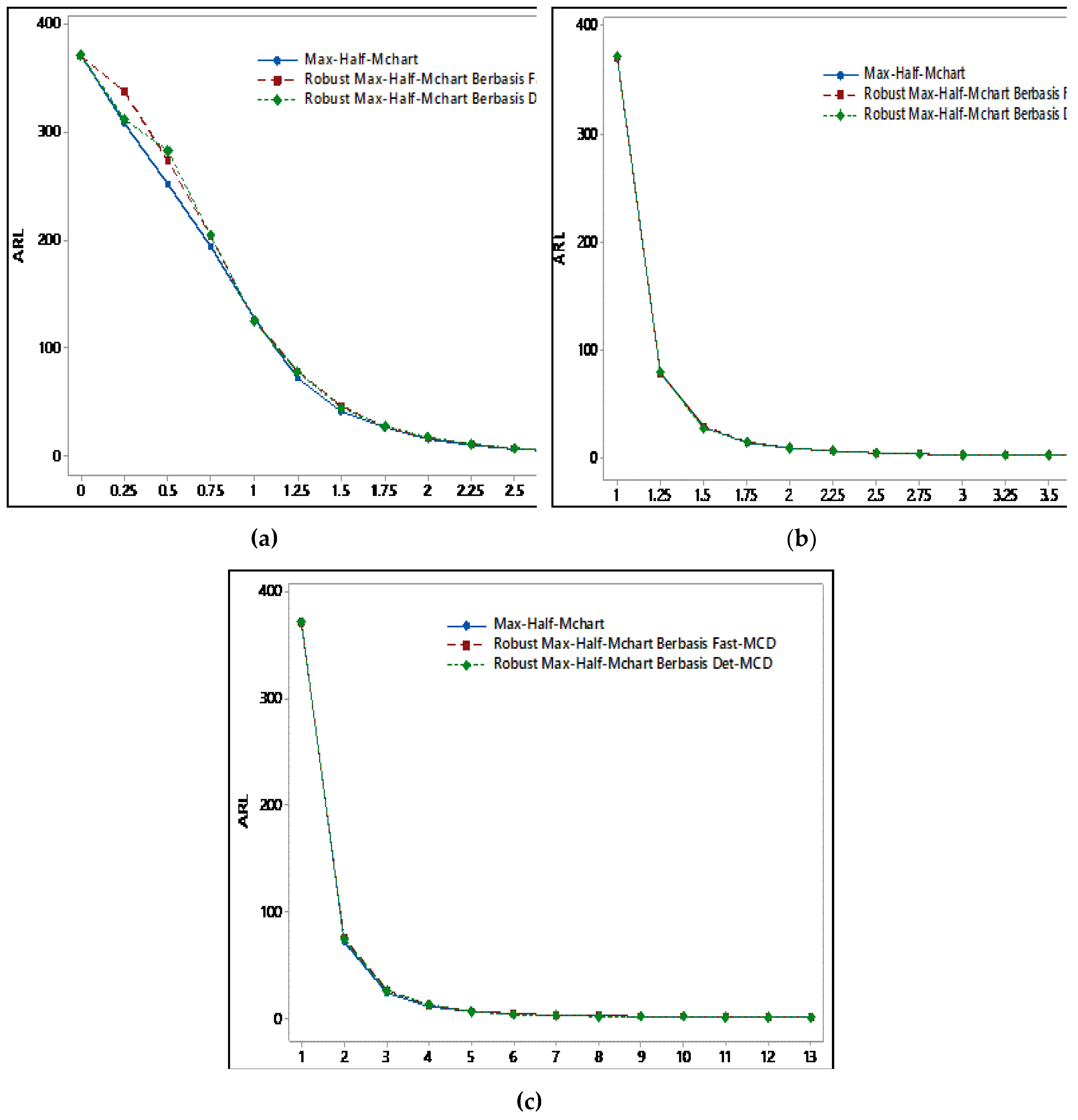
Figure 2.
Accuracy Perfomance for All Charts for Mean and Covariance Matrix Shift Based on Various Correlation a) 0.3, (b) 0.5, (c) 0.7.
Figure 2.
Accuracy Perfomance for All Charts for Mean and Covariance Matrix Shift Based on Various Correlation a) 0.3, (b) 0.5, (c) 0.7.
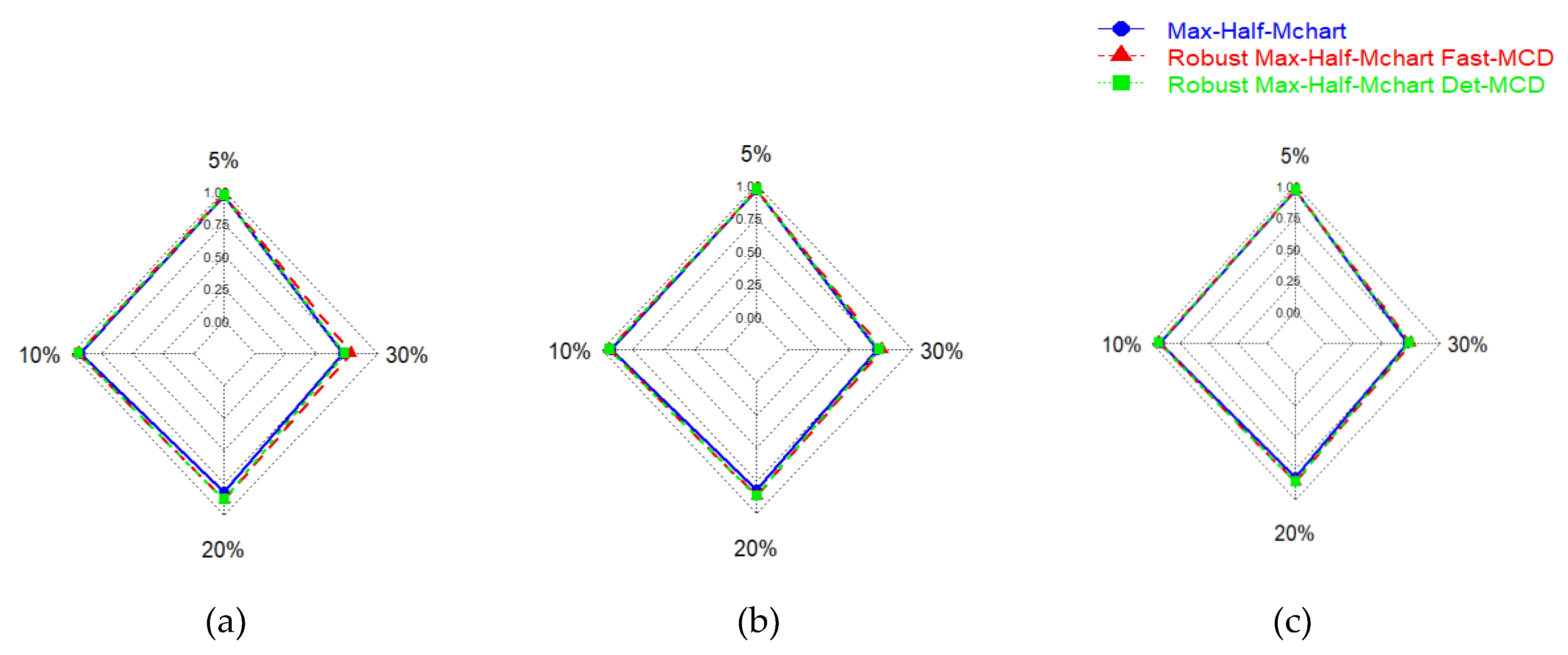
Figure 3.
FP Rate for All Charts for Mean and Covariance Matrix Shift Based on Various Correlation a) 0.3, (b) 0.5, (c) 0.7.
Figure 3.
FP Rate for All Charts for Mean and Covariance Matrix Shift Based on Various Correlation a) 0.3, (b) 0.5, (c) 0.7.
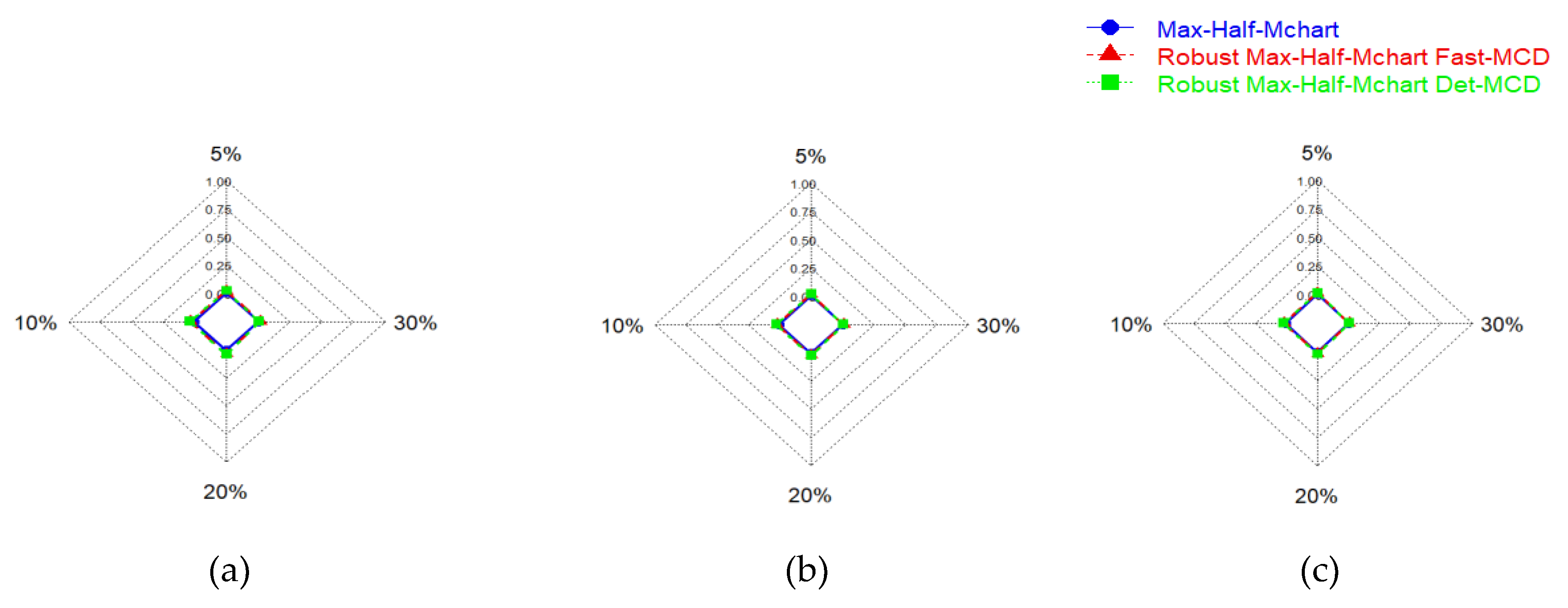
Figure 4.
FN Rate for All Charts for Mean and Covariance Matrix Shift Based on Various Corrlaltion a) 0.3, (b) 0.5, (c) 0.7.
Figure 4.
FN Rate for All Charts for Mean and Covariance Matrix Shift Based on Various Corrlaltion a) 0.3, (b) 0.5, (c) 0.7.
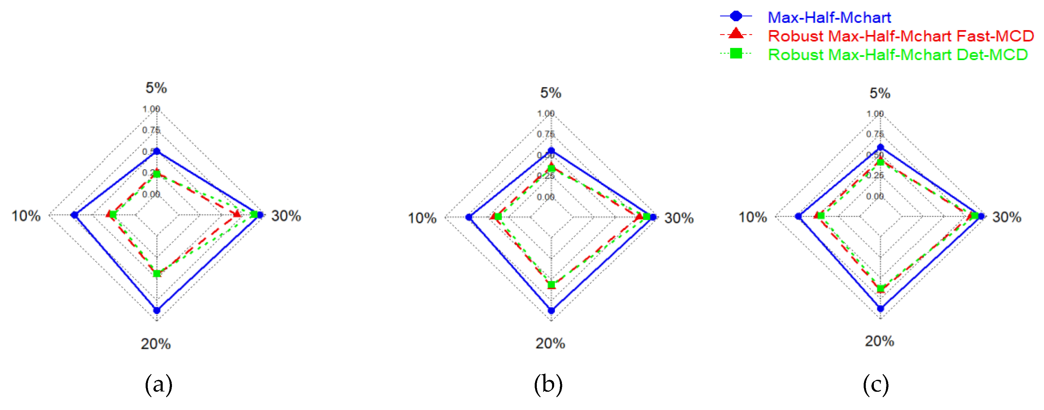
Figure 5.
AUC Rate for All Charts for Mean and Covariance Matrix Shift Based on Various Correlation a) 0.3, (b) 0.5, (c) 0.7.
Figure 5.
AUC Rate for All Charts for Mean and Covariance Matrix Shift Based on Various Correlation a) 0.3, (b) 0.5, (c) 0.7.
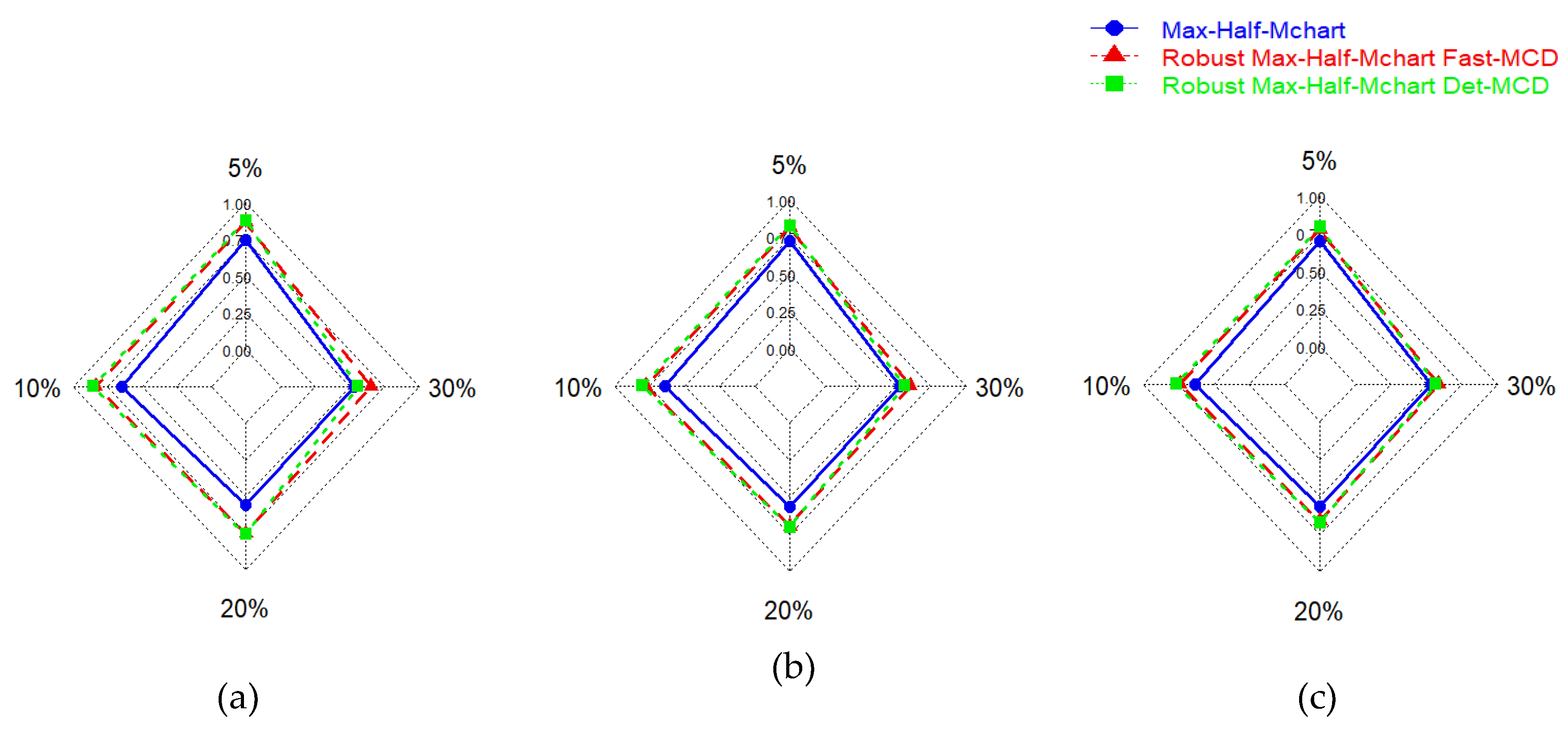
Figure 6.
Statistics Plot of Simulation with 5% Outlier using (a) Max-Half-Mchart (b) Max-Half-Mchart -FMCD (c) Max-Half-Mchart-DMCD.
Figure 6.
Statistics Plot of Simulation with 5% Outlier using (a) Max-Half-Mchart (b) Max-Half-Mchart -FMCD (c) Max-Half-Mchart-DMCD.
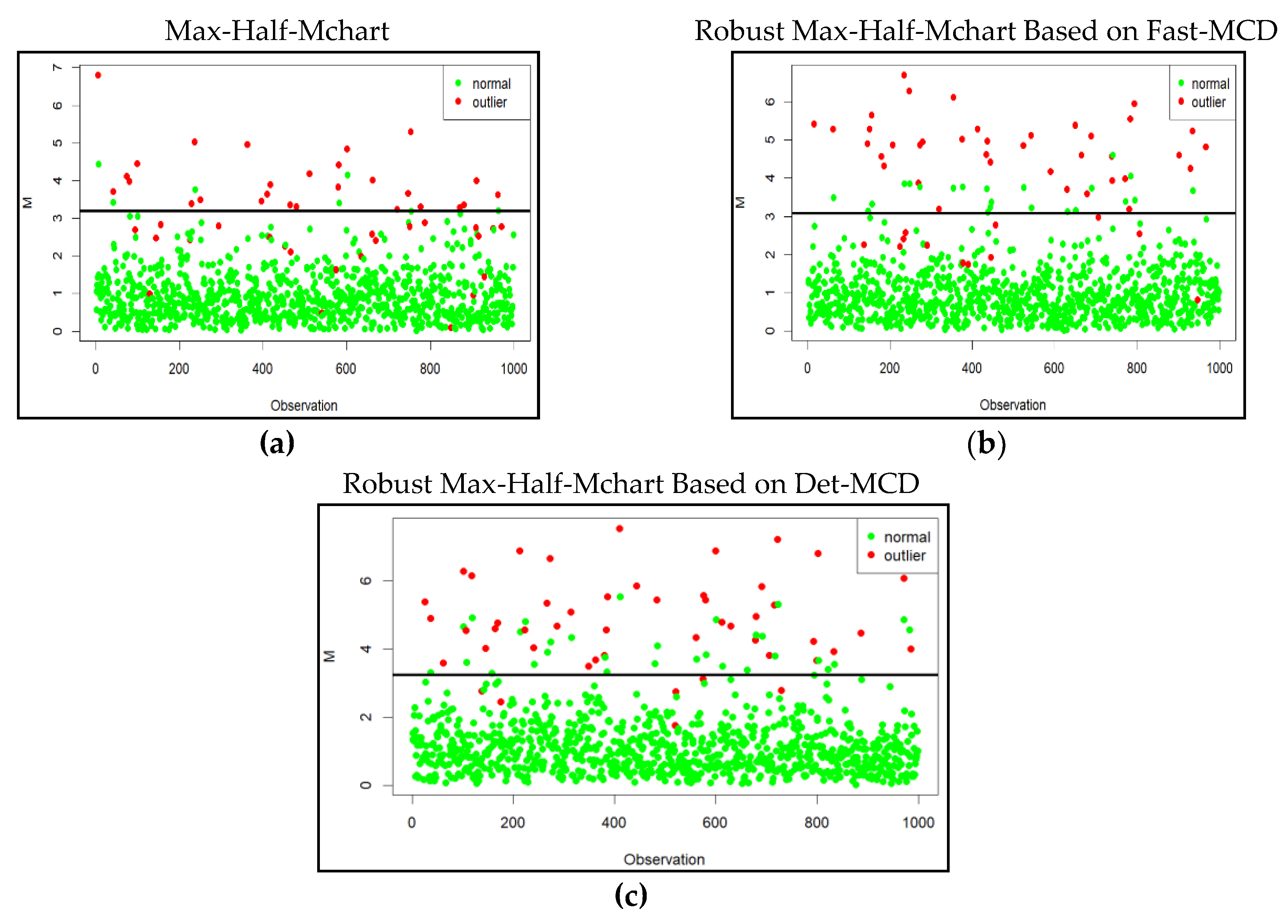
Figure 7.
Statistics Plot of Simulation with 10% Outlier using (a) Max-Half-Mchart (b) Max-Half-Mchart -FMCD (c) Max-Half-Mchart-DMCD.
Figure 7.
Statistics Plot of Simulation with 10% Outlier using (a) Max-Half-Mchart (b) Max-Half-Mchart -FMCD (c) Max-Half-Mchart-DMCD.
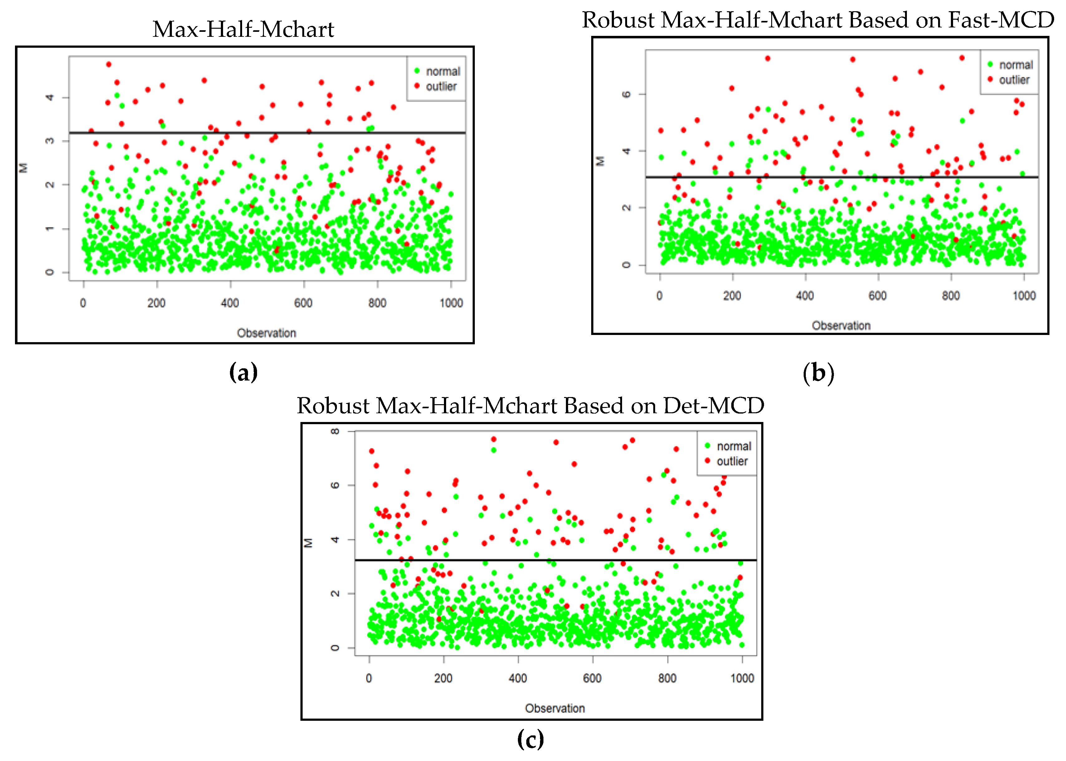
Figure 8.
Statistics Plot of Simulation with 20% Outlier using (a) Max-Half-Mchart (b) Max-Half-Mchart -FMCD (c) Max-Half-Mchart-DMCD.
Figure 8.
Statistics Plot of Simulation with 20% Outlier using (a) Max-Half-Mchart (b) Max-Half-Mchart -FMCD (c) Max-Half-Mchart-DMCD.
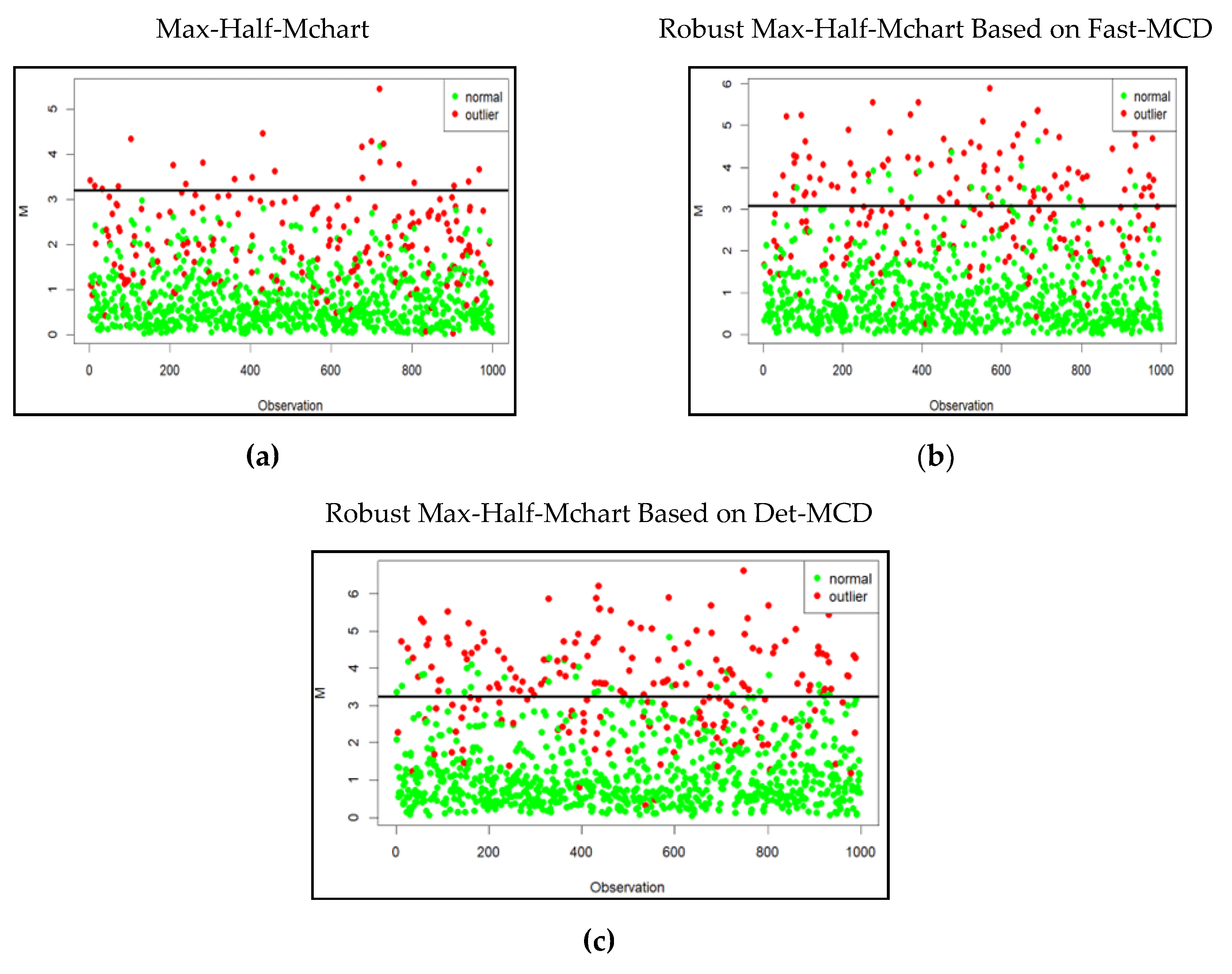
Figure 9.
Statistics Plot of Simulation with 30% Outlier using (a) Max-Half-Mchart (b) Max-Half-Mchart -FMCD (c) Max-Half-Mchart-DMCD.
Figure 9.
Statistics Plot of Simulation with 30% Outlier using (a) Max-Half-Mchart (b) Max-Half-Mchart -FMCD (c) Max-Half-Mchart-DMCD.
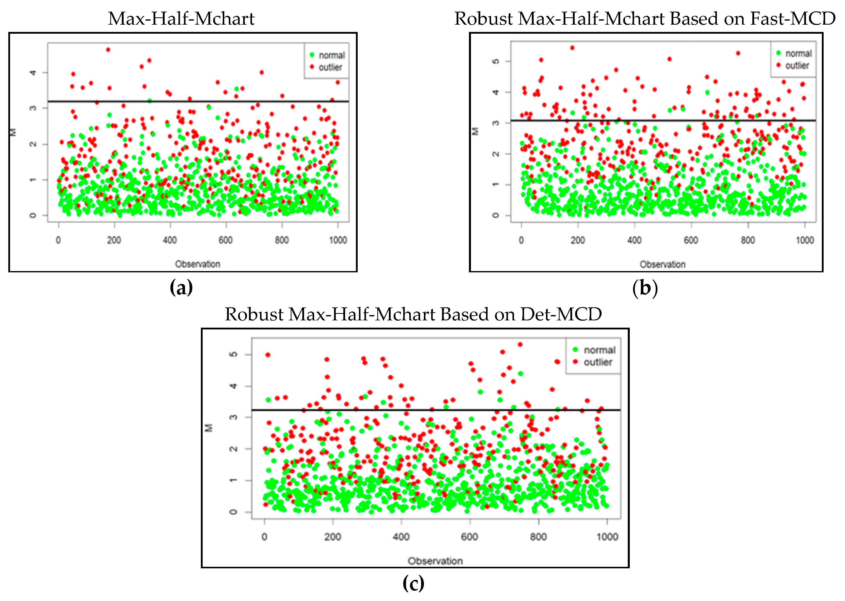
Figure 10.
Max-Half-Mchart Statistic Plot.
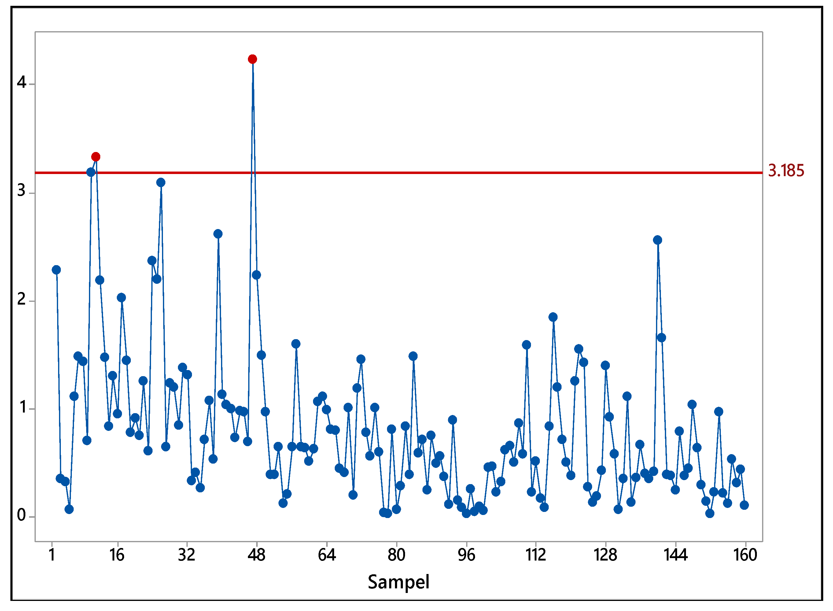
Figure 11.
Max-Half-Mchart Based on Fast-MCD Statistic Plot.
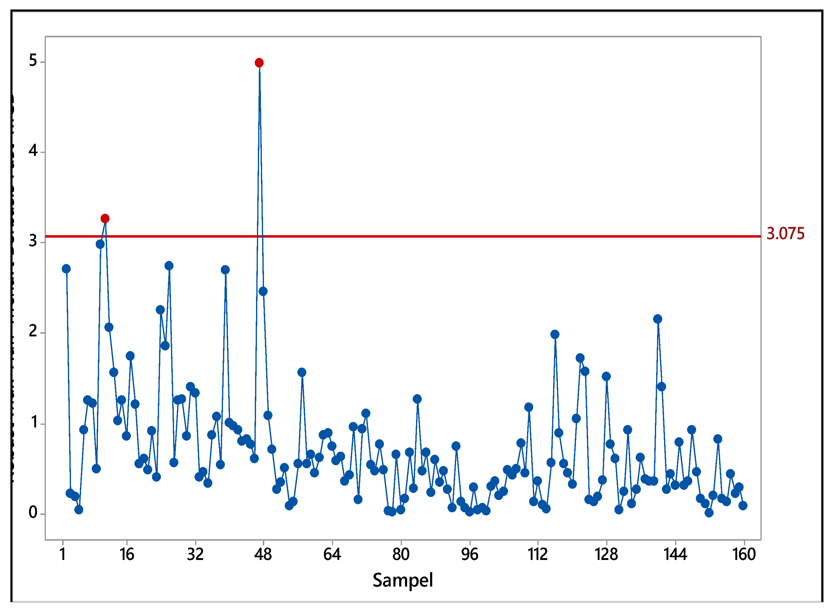
Figure 12.
Max-Half-Mchart Statistic Plot.
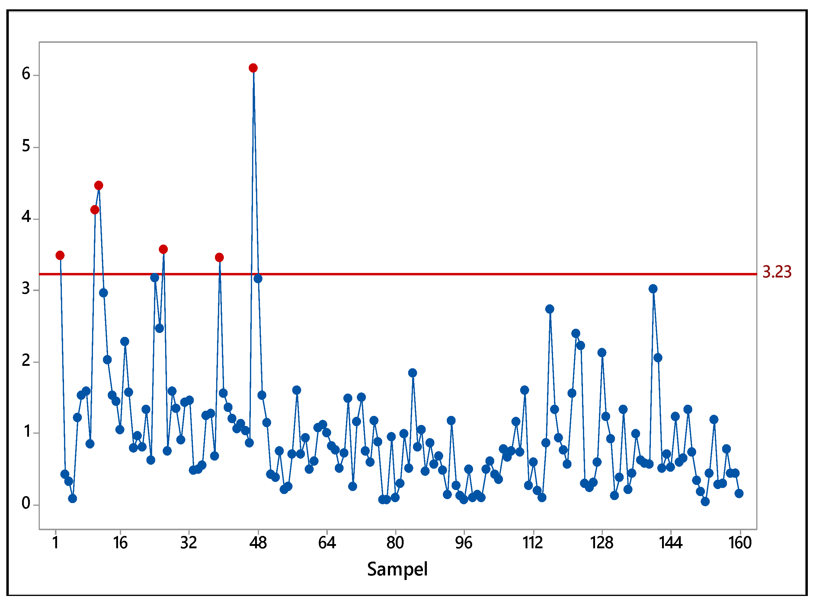
Table 1.
Performance. ARL Simulation with Correlation Levels
| a | b | |||||||||||||||||||||||||
| 1 | 1.25 | 1.5 | 1.75 | 2 | 2.25 | 2.5 | 2.75 | 3 | 3.25 | 3.5 | 3.75 | 4 | ||||||||||||||
| 0 | 372.94 | 80.06 | 28.39 | 14.18 | 8.91 | 6.00 | 4.67 | 3.37 | 2.95 | 2.54 | 2.22 | 2.00 | 1.85 | |||||||||||||
| 371.13 | 80.56 | 29.22 | 14.51 | 9.41 | 6.22 | 4.63 | 3.84 | 3.02 | 2.57 | 2.25 | 2.17 | 1.88 | ||||||||||||||
| 371.37 | 73.93 | 28.84 | 13.90 | 9.05 | 5.86 | 4.55 | 3.62 | 3.08 | 2.54 | 2.30 | 2.08 | 1.90 | ||||||||||||||
| 0.25 | 310.41 | 72.76 | 26.31 | 13.54 | 8.58 | 5.78 | 4.60 | 3.66 | 2.85 | 2.53 | 2.20 | 2.00 | 1.85 | |||||||||||||
| 326.69 | 70.36 | 28.05 | 13.81 | 8.47 | 5.83 | 4.53 | 3.53 | 2.92 | 2.50 | 2.24 | 1.97 | 1.88 | ||||||||||||||
| 311.68 | 69.71 | 26.05 | 14.27 | 8.31 | 5.84 | 4.38 | 3.45 | 2.99 | 2.52 | 2.21 | 2.03 | 1.87 | ||||||||||||||
| 0.5 | 215.25 | 52.65 | 22.32 | 12.56 | 7.71 | 5.41 | 4.12 | 3.30 | 2.77 | 2.50 | 2.13 | 1.98 | 1.75 | |||||||||||||
| 222.40 | 59.14 | 23.22 | 12.57 | 7.86 | 5.30 | 4.01 | 3.28 | 2.82 | 2.43 | 2.23 | 1.96 | 1.85 | ||||||||||||||
| 232.42 | 58.44 | 22.56 | 12.00 | 7.81 | 5.62 | 4.36 | 3.29 | 2.95 | 2.52 | 2.24 | 1.86 | 1.82 | ||||||||||||||
| 0.75 | 122.80 | 39.15 | 17.88 | 10.65 | 6.81 | 4.88 | 3.61 | 3.06 | 2.57 | 2.23 | 2.13 | 1.89 | 1.71 | |||||||||||||
| 129.17 | 39.18 | 18.81 | 10.13 | 6.78 | 4.84 | 4.00 | 3.17 | 2.61 | 2.32 | 2.16 | 1.88 | 1.78 | ||||||||||||||
| 129.06 | 39.88 | 18.50 | 10.29 | 6.91 | 4.84 | 3.85 | 3.15 | 2.65 | 2.42 | 2.13 | 1.86 | 1.76 | ||||||||||||||
| 1 | 63.71 | 25.38 | 12.36 | 8.14 | 5.21 | 4.37 | 3.46 | 2.95 | 2.47 | 2.18 | 1.99 | 1.77 | 1.64 | |||||||||||||
| 65.58 | 23.70 | 12.51 | 8.22 | 5.65 | 4.39 | 3.38 | 2.81 | 2.54 | 2.25 | 2.00 | 1.80 | 1.71 | ||||||||||||||
| 72.91 | 25.60 | 12.34 | 7.97 | 5.56 | 4.20 | 3.28 | 2.83 | 2.57 | 2.23 | 1.97 | 1.79 | 1.75 | ||||||||||||||
| 1.25 | 31.20 | 14.70 | 8.63 | 6.25 | 4.37 | 3.48 | 3.04 | 2.63 | 2.29 | 1.97 | 1.85 | 1.68 | 1.60 | |||||||||||||
| 31.82 | 15.46 | 9.08 | 6.34 | 4.69 | 3.55 | 2.99 | 2.47 | 2.23 | 2.05 | 1.81 | 1.77 | 1.64 | ||||||||||||||
| 32.66 | 15.69 | 9.14 | 6.13 | 4.60 | 3.74 | 3.01 | 2.48 | 2.27 | 2.02 | 1.77 | 1.74 | 1.62 | ||||||||||||||
| 1.5 | 16.26 | 8.80 | 6.37 | 4.23 | 3.53 | 3.02 | 2.51 | 2.20 | 1.94 | 1.81 | 1.71 | 1.59 | 1.48 | |||||||||||||
| 16.50 | 9.28 | 6.15 | 4.76 | 3.64 | 3.03 | 2.49 | 2.30 | 2.10 | 1.87 | 1.68 | 1.61 | 1.56 | ||||||||||||||
| 16.76 | 9.00 | 6.05 | 4.65 | 3.85 | 3.03 | 2.56 | 2.21 | 1.97 | 1.83 | 1.73 | 1.57 | 1.49 | ||||||||||||||
| 1.75 | 8.44 | 5.37 | 4.35 | 3.26 | 2.93 | 2.50 | 2.21 | 1.97 | 1.79 | 1.69 | 1.56 | 1.47 | 1.46 | |||||||||||||
| 8.97 | 5.83 | 4.30 | 3.39 | 3.01 | 2.34 | 2.24 | 1.88 | 1.80 | 1.66 | 1.57 | 1.48 | 1.46 | ||||||||||||||
| 8.66 | 5.69 | 4.37 | 3.47 | 2.90 | 2.54 | 2.12 | 2.05 | 1.84 | 1.67 | 1.62 | 1.52 | 1.42 | ||||||||||||||
| 2 | 5.26 | 3.91 | 3.18 | 2.66 | 2.30 | 2.12 | 1.95 | 1.85 | 1.63 | 1.51 | 1.43 | 1.43 | 1.38 | |||||||||||||
| 5.08 | 3.78 | 3.19 | 2.66 | 2.36 | 2.08 | 1.96 | 1.79 | 1.63 | 1.57 | 1.51 | 1.43 | 1.37 | ||||||||||||||
| 5.23 | 3.95 | 3.29 | 2.68 | 2.34 | 2.15 | 1.90 | 1.82 | 1.70 | 1.53 | 1.49 | 1.41 | 1.40 | ||||||||||||||
| a | b | |||||||||||||||||||||||||
| 1 | 1.25 | 1.5 | 1.75 | 2 | 2.25 | 2.5 | 2.75 | 3 | 3.25 | 3.5 | 3.75 | 4 | ||||||||||||||
| 2.25 | 3.37 | 2.73 | 2.35 | 2.11 | 1.92 | 1.75 | 1.67 | 1.51 | 1.50 | 1.43 | 1.37 | 1.33 | 1.25 | |||||||||||||
| 3.33 | 2.66 | 2.53 | 2.19 | 1.95 | 1.81 | 1.69 | 1.56 | 1.47 | 1.41 | 1.38 | 1.34 | 1.31 | ||||||||||||||
| 3.33 | 2.81 | 2.35 | 2.19 | 1.93 | 1.81 | 1.63 | 1.57 | 1.44 | 1.42 | 1.35 | 1.38 | 1.30 | ||||||||||||||
| 2.5 | 2.41 | 2.07 | 1.92 | 1.73 | 1.62 | 1.63 | 1.52 | 1.45 | 1.36 | 1.39 | 1.33 | 1.24 | 1.24 | |||||||||||||
| 2.37 | 2.04 | 1.90 | 1.78 | 1.70 | 1.53 | 1.50 | 1.44 | 1.36 | 1.32 | 1.27 | 1.31 | 1.23 | ||||||||||||||
| 2.43 | 2.03 | 1.90 | 1.75 | 1.63 | 1.57 | 1.54 | 1.49 | 1.40 | 1.33 | 1.30 | 1.26 | 1.23 | ||||||||||||||
| 2.75 | 1.72 | 1.72 | 1.54 | 1.48 | 1.47 | 1.34 | 1.35 | 1.28 | 1.32 | 1.25 | 1.21 | 1.20 | 1.19 | |||||||||||||
| 1.72 | 1.71 | 1.59 | 1.50 | 1.49 | 1.44 | 1.36 | 1.36 | 1.27 | 1.24 | 1.22 | 1.21 | 1.19 | ||||||||||||||
| 1.77 | 1.67 | 1.58 | 1.51 | 1.50 | 1.45 | 1.35 | 1.33 | 1.28 | 1.26 | 1.21 | 1.26 | 1.19 | ||||||||||||||
| 3 | 1.42 | 1.34 | 1.33 | 1.28 | 1.30 | 1.30 | 1.24 | 1.24 | 1.19 | 1.17 | 1.16 | 1.15 | 1.13 | |||||||||||||
| 1.44 | 1.43 | 1.37 | 1.31 | 1.35 | 1.30 | 1.30 | 1.22 | 1.19 | 1.18 | 1.16 | 1.14 | 1.16 | ||||||||||||||
| 1.43 | 1.40 | 1.36 | 1.31 | 1.33 | 1.28 | 1.26 | 1.22 | 1.21 | 1.18 | 1.18 | 1.16 | 1.13 | ||||||||||||||
Table 7.
Amount of data Out-of-Control and In-Control on Robust Max-Half-Mchart and Max-Half-Mchart
| Control Chart | Out-of-Control | Mean Shift | Variability Shift |
| Max-Half-Mchart | 2 | 2 | 0 |
|
Robust Max-Half-Mchart Based on Fast-MCD |
2 | 2 | 0 |
|
Robust Max-Half-Mchart Based on Det-MCD |
6 | 4 | 2 |
Disclaimer/Publisher’s Note: The statements, opinions and data contained in all publications are solely those of the individual author(s) and contributor(s) and not of MDPI and/or the editor(s). MDPI and/or the editor(s) disclaim responsibility for any injury to people or property resulting from any ideas, methods, instructions or products referred to in the content. |
© 2026 by the authors. Licensee MDPI, Basel, Switzerland. This article is an open access article distributed under the terms and conditions of the Creative Commons Attribution (CC BY) license (http://creativecommons.org/licenses/by/4.0/).
Copyright: This open access article is published under a Creative Commons CC BY 4.0 license, which permit the free download, distribution, and reuse, provided that the author and preprint are cited in any reuse.


