

Submitted:
06 February 2026
Posted:
09 February 2026
You are already at the latest version
Abstract
The article examines the persistent stability of weighted average cost of capital (WACC) disclosed by German DAX40 companies despite substantial declines in risk-free interest rates between 2004 and 2021. While theory suggests that WACC should reflect lower risk-free interest rates and decline as well with falling government bond yields, empirical evidence reveals minimal adjustment in reported WACC figures. Disclosed WACC of DAX40 companies remain between 7% and 8% as the yield of the ten-year German government bond fell from 4.1% to –0.2%. This study employs quantitative analyses to investigate whether systematic increases in risk exposure can explain this phenomenon. Using capital market data spanning from 2000 to 2023, we analyze five risk dimensions: systematic risk (beta factors), overall market volatility, risk aversion (lambda factors), earnings risk, and financial structure risk. Bootstrap analyses reveal a 41.5% reduction in beta factor variance, while volatility analyses demonstrate declining market risk exposure. The market price of risk analysis does not reveal definite findings. Earnings risk measures indicate improved financial stability, and debt ratios show modest declines. These findings suggest that observable risk parameters cannot explain persistent WACC levels, indicating a disconnect between theoretical WACC calculations and practitioner applications in investment project decision-making following value-based management principles.
Keywords:
WACC
; portfolio theory
; investment behavior
; risk management
; interest environment
; value-based management
; capital resource allocation
; project appraisal
; risk-free interest rate
1. Introduction
The weighted average cost of capital (WACC) represents a fundamental parameter in corporate investment practices, serving as the minimum required rate of return and the appropriate discount rate for investment project calculation and resource allocation. Economic value creation, commonly measured through metrics such as economic value added (EVA), relies explicitly on accurate WACC computation. Consequently, estimation errors in WACC can systematically bias capital allocation decisions, potentially leading to suboptimal investment behavior that fails to maximize net present value (NPV) realization. The WACC theory thus provides the analytical foundation for evaluating risk-return tradeoffs in corporate decision-making contexts.
Theory posits that declining risk-free interest rates should mechanically reduce capital cost estimates, thereby expanding the set of value-creating investment opportunities. In this study, risk-free rates are proxied by yields on ten-year German government bonds, which declined from 4.1% to –0.2% between 2004 and 2021. Considering WACC definition, such substantial reductions in the risk-free component should correspond to proportional declines in overall capital costs, assuming constant risk premiums. However, empirical analysis of disclosed WACC from German DAX40 companies reveals persistent stability, with reported values remaining within a narrow 7% to 8% range from 2004 to 2021 (Figure 1). This observed stability suggests either systematic increases in risk premiums sufficient to offset declining risk-free interest rates or potential deviations from theoretically consistent WACC estimation practices. After 2021 it becomes evident that practitioners increase WACC in response to increasing risk-free interest rates, which is not investigated in the present study.
The persistent stability of WACC despite substantial variation in risk-free interest rates represents a phenomenon that warrants systematic investigation. Understanding this empirical divergence in WACC estimation practices has direct implications for capital allocation efficiency and value-based management practice.
This research comprises two complementary components designed to identify root causes and implications of persistent WACC levels in a declining interest rate environment. The study applies quantitative methods grounded in modern portfolio theory to examine whether observable risk parameters can explain the stability of reported WACC figures. Specifically, we analyze five risk dimensions using capital market data and fundamental financial information: (1) beta factors measuring systematic risk exposure relevant in WACC determinations; (2) overall market risk measured by volatility; (3) risk aversion proxied by lambda factors, (4) earnings risks expressed through EBIT volatility, and (5) financial structure risks measured by debt ratios. A complementary study (part 2) employs qualitative research methods to investigate behavioral and managerial determinants that may influence WACC estimation practices among corporate practitioners (the research is presented in a future article of JFRM). Together, these investigations provide a comprehensive examination of the divergence between theoretically correct WACC computations and observed WACC computation in practice.
This study aims to demonstrate that observable risk parameters, as measured through conventional portfolio theory factors, cannot explain the persistent WACC levels reported by German DAX40 companies during the period from 2004 to 2021.
Hence section 2 presents the research design, including underlying assumptions and testable hypotheses. Section 3 defines the risk parameters examined and describes the analytical methodologies employed. Section 4 reports the empirical findings and evaluates their implications for understanding persistent WACC levels. Section 5 concludes with a synthesis of key findings and discusses directions for the complementary qualitative expert research to be addressed in part II of this article series.
2. Problem Statement and Research Approach
Prior research examining WACC estimation practices has emphasized two primary insights: Limitations of the capital asset pricing model (CAPM) and its modifications for generating risk-adjusted discount rates, and alternative methodological approaches employed by practitioners in corporate capital cost determination (Damodaran, 2022; Ross, 1976; Fama/French, 1992; Carhart, 1997; Koedijk/Van Dijk, 2004; Dumas/Solnik, 1995; Santis/Gerard, 1997; Merton, 1997). Within the theoretical conception of portfolio theory, declining risk-free interest rates should correspond to reductions in WACC, while holding risk premiums constant. Consequently, the empirical phenomenon implies either systematic increases in risk exposures sufficient to offset lower risk-free rates, or potential deviations from theoretically consistent estimation practices. Several studies have documented the sensitivity of required returns to interest rate environments (Farooq et al., 2021; Frank/Shen, 2016; Saleheen et al., 2017), though the specific mechanisms linking interest rate changes to risk premium adjustments remain not entirely understood.
To quantitatively analyze this phenomenon, disclosed WACC of DAX40 companies are decomposed into risk-free and risk premium components. The risk premium is computed as the difference between reported WACC and the ten-year German government bond yield. Figure 2 depicts this decomposition by distinguishing between two risk premium measures: a constant premium fixed at the 2004 level (serving as a baseline reference), and an implicit premium representing the additional risk premium required to reconcile observed WACC with declining risk-free interest rates. This implicit premium, which equals zero by construction in the 2004 base year, reaches a maximum of 4.2% in 2020 before declining slightly to 4.0% in 2021. This observation suggests that implied risk premiums increased in line to offset declining risk-free rates, maintaining largely stable WACC figures. Whether this pattern reflects an actual increase in systematic risk for companies and managers or is instead an implicit manipulation of estimation methods is the central empirical question that motivates this study.
Figure 2 implies the motivation for three interrelated research questions. First, have systematic risk exposures relevant to WACC levels increased sufficiently to justify stable capital cost estimates despite declining risk-free interest rates? Second, what causes can explain observed deviations between WACC figures employed in corporate investment decision-making and theoretically consistent estimates derived from capital market data? Third, what implications (strengths/weaknesses) do theory-practice WACC-deviations have for corporate investment decisions and value creation capabilities?
This article primarily addresses the first two research questions through hypothesis-driven empirical analysis. Modern portfolio theory provides the established theoretical framework linking systematic risk measures to required returns. The existence of well-developed theoretical frameworks enables rigorous empirical testing of whether observable risk parameters can explain persistent WACC levels (Klandt/Heidenreich, 2017).
According to the WACC theory, the observed increasing discrepancy between varying risk-free interest rates and largely stable capital costs implies increase in individual risk exposure. In this context Saleheen/Levina (2017) state that increased risk premiums may have offset the mechanical effects of lower risk-free interest rates on WACC. Additionally, Lehmann (2019) documents that investors have apparently made little adjustment to their return requirements.
Given that risk-free interest rate proxies using government bond yields are well-recognized and largely uncontroversial in both academic literature and practice, this study examines whether observable risk parameters derived from capital market data exhibit systematic changes sufficient to explain persistent WACC levels. Due to DAX40 companies operate globally, this study incorporates relevant market indices and its constitutent companies.
3. Materials and Methods
3.1. Research Hypotheses and Data Basis
Within the CAPM, systematic risk is captured through beta coefficients, which measures the covariance between individual stock returns and market portfolio returns. Beyond the beta factor analysis, a comprehensive risk assessment involves evaluation of overall market risk, risk aversion, firm-specific earnings volatility, and financial structure risks. This study tests five hypotheses corresponding to these risk dimensions:
- H1)
- Relevant risk of the company’s shares, estimated using the beta factor of the CAPM, has increased.
- H2)
- Total market risk exposure of the stock market expressed in terms of volatility has increased.
- H3)
- Risk aversion and thus the “market price of risk” (i.e. lambda factor λ) has increased.
- H4)
- Earnings risk of companies, measured by EBIT volatility, has increased.
- H5)
- Financial structure risk, measured by the proportion of borrowed capital, has changed in a way that increases WACC.
Hypotheses H1 to H5 are tested using both capital market (stock prices and index levels) data and fundamental financial data (financial statement information). Table 1 lists the market indices used as proxies for the market portfolio, specified through Reuters Instrument Codes (RIC), data retrieval dates, and institutions providing information on index composition. Retrieval dates are relevant for determining index composition, as constituent firms vary over time based on market capitalization rankings.
Capital market data are obtained from Yahoo Finance and Google Finance databases. Data retrieval is implemented programmatically using the yfinance Python API (version 0.2.18), enabling automated extraction and processing of historical price data. Stock data and index levels are identified using RIC – Refinitiv’s standardized identification system for financial instruments (Refinitiv, 2022).
3.2. H1: Analysis of the Relevant Share Risk of Companies
Beta factors serve as well-established measures of systematic risk suitable for conducting empirical tests (Bilinski/Lyssimachou, 2014).
3.2.1. Computation
Beta computation requires three key methodological specifications: (1) the selected market index serving as proxy for the market portfolio, (2) the return observation frequency (daily, weekly, or monthly), and (3) the time horizon over which price volatilities are measured. In practice, beta factors are typically determined using ex-post return data. Beta factors are estimated via OLS regression using weekly returns over rolling five-year windows (2000-2023). Data are retrieved from Yahoo Finance and Google Finance APIs, with STOXX Europe600 data sourced exclusively from Google Finance due to availability constraints. Computations are implemented in Python, storing results in DataFrame structures for subsequent analysis.
3.2.2. Analyses
Distributional analysis examines temporal changes via three metrics: mean-median difference (measuring skewness), interquartile range (IQR), and outlier frequency (defined as values beyond 1.5×IQR from quartiles). Positive mean-median differences indicate right-skewed distributions with high-beta firms, while negative values indicate left-skewed distributions dominated by low-beta firms. Increases in these parameters would signal rising systematic risk exposure. Increases in distributional parameters would indicate rising systematic risk exposure among publicly traded firms. A positive mean-median difference indicates right-skewed beta distributions, suggesting the presence of high-beta firms whose returns exhibit greater sensitivity to market movements than the average firm. Conversely, negative mean-median differences indicate left-skewed distributions, reflecting a preponderance of low-beta firms with attenuated market sensitivities.
Confidence intervals provide additional distributional information beyond point estimates. A () confidence interval indicates that the true population parameter lies within the interval bounds with probability () (Dreger, 2014). For this study, 95% confidence intervals are computed using the percentile method, implemented in Python as follows:
confidence_interval_95 = np.nanpercentile(daxbeta[„2000”],[2.5, 97.5])
Bootstrap analysis. Bootstrap resampling provides a non-parametric procedure for statistical inference that does not rely on distributional assumptions about the underlying data. Bootstrap samples are generated through repeated random sampling with replacement from the empirical distribution (Horowitz, 2001; Hall, 1992). Each bootstrap sample contains data points (where corresponds to the sample size), from which the mean and variance are computed as bootstrap estimates (Good, 2000). Repeating this procedure times yields bootstrap replications of the statistic of interest. This study implements bootstrap procedures with replications (see Figure 3).
Hypothesis testing. To examine temporal changes in systematic risk expressed by beta factors, hypothesis tests are performed in conjunction with bootstrapping. Specifically, the 2023 beta distribution for each index is compared against distributions from each prior year using one-sided tests of the null hypothesis that mean beta values are unchanged: versus . For bootstrap hypothesis tests, the null hypothesis of equal means is imposed by recentering both samples around their pooled mean, ensuring that the null hypothesis holds exactly in the resampled data (Klandt/Heidenreich, 2017). Bootstrap samples are then drawn from these recentered distributions, and the distribution of the test statistic under the null is estimated empirically (MacKinnon/James, 2007).
3.2.3. Unlevered Beta Factor
Beta factors estimated from stock returns and market returns reflect both business risk and financial risk induced by leverage and are therefore referred to as levered betas. Unlevered beta factors measure the systematic risk of a company’s assets independent of its financing choices, corresponding conceptually to the beta of 100% equity-financed company (Pratt/Grabowski, 2014). Beta factors are unlevered to isolate systematic business risk from capital structure effects and comprehensively answer hypothesis H1 of this study. Two unlevering approaches are employed: the Hamada formula and the Harris/Pringle formula, each differing in their treatment of tax shields (Enzinger/Kofler, 2011).
The result of unlevering comprises four unlevered beta factor series for each firm: (1) according to Hamada with book values of capital sources; (2) according to Hamada with market values of capital sources; (3) according to Harris/Pringle with book values of capital sources; and (4) according to Harris/Pringle with market values of capital sources.
Leverage ratios are computed using five-year rolling averages to match the temporal structure of beta computation windows.
Unlevered beta series are evaluated using two metrics: the coefficient of variation (CV) and variance of beta estimates over time.
3.3. H2: Analysis of the Overall Market Risk Exposure
As economic uncertainty (expressed as market volatility) increases, return predictability diminishes, inducing higher required risk premiums and thus could provide an explanation for the observed phenomenon. Market volatility influences WACC through two channels: Directly through the market risk premium component in the CAPM, and indirectly through its effect on estimated beta coefficients, both of which are functions of return variance and covariance structures.
Substantial empirical evidence documents the effect of market volatility on the WACC. Brotherson et al. (2013) find that volatile capital markets complicate market risk premium estimation in practice. Poterba and Summers’ (1995) study reveals that approximately 20% of companies would abandon a net present value (NPV)-positive investment project if this resulted in adverse stock market reactions. Bertram et al. (2015) explain that capital costs are driven by the observable increase in volatility in bond and stock markets. Bansal et al. (2012) estimate that volatility risks account for approximately half of the equity risk premium demanded by equity investors, highlighting its economic significance for expected returns. In addition, numerous studies show negative relationships between measures of investor uncertainty and stock returns (Ang et al., 2006; Diether et al., 2002; Johnson, 2004; Larson/Resutek, 2017).
3.3.1. Computation
Hypothesis H2 tests whether increased volatility explains WACC persistence. Volatility is computed as the standard deviation of logarithmic daily returns over rolling 20-day windows beginning in 2000, ending in 2022. Albrecht/Maurer, 2016):
Stock price data are imported into GoogleColab using Python. The Yahoo Finance API is used for S&P500, FTSE100, and SMI. The DAX40 index, a total return index incorporating dividends and other income, requires separate data sourcing from Google Finance due to unavailability on Yahoo Finance. Similarly, STOXX Europe600 price data are obtained through Google Finance.
3.3.2. Analyses
Distributional analysis examines IQR, median, and outlier frequency via linear regression. Retrosprective volatility analysis assesses whether historical volatility (5-10 years) reliably forecasts realized volatility since analysts and investors commonly utilize historical capital market data to estimate expected values and to anticipate future financial events. For example, historical capital market data are used to quantify risks in the context of company valuations (Gleißner, 2014).
Consider an investor who estimates expected market risk (expressed through volatility) for a given using historical average from a specific period beginning in and ending in , where . One may question whether the quality of such historical estimates has deteriorated over time, potentially contributing to higher perceived uncertainty among market participants. This analysis examines whether historical volatility serves as a reliable estimator of expected volatility for (see Figure 4).
Average volatilities for each index are computed over rolling five- to ten-year periods, denoted . These historical averages are compared to the volatility of a defined forecast year () to derive absolute and relative volatility buffers:
A negative indicates that volatility in the forecast year exceeds the historical average, suggesting that forecast models may underestimate market risk, possibly leading to suboptimal investment decisions.
The examination of distributions and occurrence probabilities of negative (nBR) and positive (pBR) volatility buffer ratios addresses the following key question: what is the probability that expected volatility surpasses historical values, thereby exposing investors to downside risk? Greater probabilities of nBR may indicate increased investor perception of shortfall risk, which could manifest as higher implied risk premiums. Probability distributions of BR, nBR, and pBR are created using kernel density estimation (KDE). Assuming normality, occurrence probabilities are computed by fitting normal distributions to empirical means and standard deviations of volatility buffers for each index. The data range is segmented into ten equal intervals, with probabilities calculated for each interval.
3.4. H3: Analysis of the Market Price of Risk
Investors return requirements are influenced not only by changes in risk levels but also by variations in risk aversion among market participants. Risk premiums compensate investors for the covariance of security returns with macroeconomic performance, particularly penalizing securities that underperform during economic downturns (Berk/DeMarzo, 2011).
3.4.1. Computation
The market price of risk denoted (lambda factor), quantifies the additional expected return investors require per unit of risk. Franzen/Schäfer (2018) describe lambda as a non-dimensional benchmark to compare portfolios:
where is the expected portfolio return (computed as a ten-year moving geometric mean, aligning with the risk-free proxy maturity), is the risk-free interest rate and is the annualized portfolio return volatility. Table 4 shows proxies for risk-free interest rate depending on the index.
The yields on ten-year and long-term government bonds were taken from Statista (Statistics Denmark 2024; Banque centrale du Luxembourg, 2024a; Österreichische Nationalbank, 2024; Banque centrale du Luxembourg, 2024b). The data for the DAX40 price index and STOXX Europe600 are retrieved via Google Finance for the period spanning from 2000 to 2023. For index levels of S&P500, FTSE100, and SMI, the Yahoo Finance API is employed.
3.4.2. Analyses
To assess whether the market price of risk represents a relevant explanatory variable for deviations between disclosed and theoretically calculated capital costs, lambda factors are examined in a regression analysis and comparative evaluation. Additionally, lambda factors are measured using varying return intervals (ranging from ten to 15 years). The sensitivity analysis varies intervals from ten to fifteen years to assess robustness, with results examined via correlation matrices.
3.5. H4: Analysis of Earnings Risks
Higher earnings risks – arising from factors such as customer concentration, order dependency, or supplier concentration – increase the probability of insolvency, thus representing existential risks for firms (Gleißner, 2014). In the context of estimating risk-adjusted cost of capital using historical stock price data, Gleißner (2014) argues that fluctuations in shareholder payments or financial surpluses are relevant for shareholders. Although publicly traded companies do not explicitly incorporate earnings risks in annual report disclosures of capital cost estimations, changes in fundamental business risks influence capital cost estimates in a declining interest rate environment. Following Gleißner’s approach, the risk premium component of cost of capital is proportional to the coefficient of variance (CV) of earnings. Thus, aggregate earnings risk directly impacts both the cost of capital and the implied risk premium (Gleißner, 2016).
3.5.1. Computation
Earnings volatility is expressed through the coefficient of variation (CV) of EBIT values:
CV normalizes absolute EBIT values for cross-company comparability. EBIT margins (EBIT/revenue) supplement absolute measures for shortfall risk assessment. Earnings risk measurement is based on earnings volatility analysis, specifically examining EBIT margin fluctuations, over five consecutive fiscal years for each company. Fundamental financial data are sourced from Pitchbook, with data availability extending back to 2000 if possible. Because earnings risks were analyzed in 2022, EBIT-based measurements cover the period through 2021. Therefore, company selection is based on the index composition as of 2022.
3.5.2. Analyses
CV is evaluated via median, IQR, and outlier regression. Due to interpretive limitations with negative EBIT values, downside risk measures (Value-at-Risk (VaR) and Conditional-Value-at-Risk (CVaR)) supplement CV analysis. Return-CVaR () is estimated through both analytical methods (historical approach and parametric variance-covariance method) and simulation-based approach (Monte Carlo method (MC)) assuming normally distributed returns from five consecutive periods. Applying the variance-covariance method, a distribution curve is constructed to calculate the return-CVaR based on the expected value and standard deviation of the historical values.
The parametric variance-covariance method parallels the historical approach, with the difference that a normal distribution of returns is assumed instead of historical data. The return-CVaR of all companies is compared for the period 2010 to 2021, with distributional statistics compared across methods.
3.6. H5: Analysis of Financial Structure Risks
When companies employ debt financing (partial or substantial), this capital structure composition influences both the expected returns and the overall risk profile. The resulting risk premium reflects both operating business risk and financial risk arising from leverage (Steiner et al., 2017).
3.6.1. Computation
Financial structure risk is measured by debt ratios (debt capital/total capital) using book-value (balance sheet) and market-value (market capitalization) approaches. Debt ratio analysis is limited to DAX40 companies, because financing risks are partially captured through earnings volatility analysis, and accordingly debt ratio analysis for cross-index comparisons would provide limited marginal insight. For DAX40 companies, debt ratios are calculated using data from audited annual reports. Market value of equity is determined by multiplying the number of outstanding shares by the closing share price on the fiscal year-end date. Book values for debt and equity are extracted directly from the balance sheet components reported in the annual reports.
3.6.3. Analyses
Both market-based and accounting-based debt ratios of DAX40 companies are examined temporally to assess potential relationships with reported WACC levels. The analysis employs graphical presentation to illustrate trends in financial leverage over the sample period.
4. Results
4.1. H1: Systematic Risk Assessment: Beta Factor Analyses
Beta factor distributions are analyzed using multiple visualization techniques by distributional parameters including means, medians, and 95% confidence intervals. Figure 5 presents the empirical evidence depicted through the mean-median difference, which measures skewness of beta distributions, and the IQR, which measures dispersion. From an investor’s perspective, increases in both parameters would indicate higher systematic risk, while decreases would indicate reduced risk exposure. A positive mean-median difference (mean median) indicates right-skewed distributions, reflecting a subset of high-beta firms with above-average market sensitivity that increases the distribution mean. Conversely, a negative difference (mean median) indicates left-skewed distributions, reflecting a preponderance of low-beta firms with below-average market sensitivity.
Linear regression analysis of these distributional indicators across the 2000 to 2023 period reveals regression slopes of –0.0021 and –0.0105 providing quantitative evidence that systematic risk exposure did not increase over the study period. Instead, the results indicate declining volatility of company share prices relative to index level movements, suggesting reduced systematic risk exposure for investors.
With bootstrap analysis, 10.000 variance beta estimates are generated through random sampling with replacement for each year’s cross-sectional beta distribution. The median of bootstrap variances provides a robust, non-parametric estimate of the central tendency of year-specific beta factor variance. Across the period of 2000 to 2023, 24 bootstrap estimates are generated to produce a time series of median bootstrap variances. Figure 6 presents the results for DAX40 companies as an illustrative example.
The empirical evidence reveals two critical findings: (1) the median bootstrap variance of DAX40 beta factors decreased substantially from 0.134 in 2000 to 0.094 in 2023, representing a 29.9% reduction in systematic risk dispersion over the 23-year period. (2) the progressive decline in median bootstrap variance indicates that the cross-sectional spread of systematic risk exposures among firms has narrowed, suggesting more homogeneous market risk profiles and reduced environmental shocks affecting individual firms.
Figure 7 shows the development of the medians of the beta variances of all indices over time and provides evidence for decreased beta factor variances across all indices. On average, from 0.176 (in 2000) to 0.103 (in 2023) – this corresponds to a reduction of 41.5%. From an investor’s perspective, this convergence in systematic risk exposures indicates a more stable or less turbulent equity market environment during the investigation period.
To assess the precision and variability of beta factor variance estimates, 95%-bootstrap confidence intervals are constructed for each year’s beta factor distribution. The confidence interval width provides a quantitative measure of the dispersion of bootstrap variance estimates. Consistent with the median variance findings, the confidence interval widths demonstrate a significant decline (see Figure 8). This convergence of confidence interval widths indicates reduced variance in systematic risk exposure and provides additional statistical support for the conclusion that cross-sectional beta factor variability has declined over time.
The bootstrap hypothesis testing compares the 2023 beta distribution against each prior year (2000 to 2022). Empirical p-values derived from 10.000 bootstrap samples range from 0.45 to 0.60 across all indices. These p-values significantly exceed the conventional significance threshold , providing strong statistical evidence that the null hypothesis cannot be rejected. This result indicates no statistically significant increase in 2023 beta factor variances relative to prior years, thereby supporting the conclusion that systematic risk exposure has not increased over time.
The unlevering procedures according to Hamada and Harris/Pringle are applied to isolate systematic business risk from financial leverage effects. Figure 9 presents the temporal development of unlevered beta coefficients of variation (CV) and variance measures. The results reveal contrasting patterns across the study period: from 2000 to 2020, both CV and variance measures demonstrate declining trends, indicating reduced variability in unlevered systematic risk exposure. However, from 2020 to 2022, both metrics increase sharply, which may be attributable to the greater uncertainty associated with the COVID-19 pandemic. Therefore, unlevered beta factors exhibit no systematic increase that could explain persistent WACC levels. An adjustment for financial leverage through unlevering procedures does not alter the conclusion derived from levered beta analyses.
Discussion in the context of the research question. Observable systematic risk cannot explain WACC persistence. Distributional and bootstrap analyses reveal declining skewness, compressed IQR, and 41.5% variance reduction—indicating reduced, not increased, risk. Unlevered beta analyses corroborate these findings. Consequently, hypothesis H1 is falsified.
4.2. H2: Overall Market Risk Exposure: Volatility Analyses
Market volatility is examined using distributional analysis, regression analysis of dispersion statistics, and retrospective evaluation of historical volatility as a predictor of investor risk expectations. Figure 10 presents box plots illustrating volatility distributions across indices. The figure reveals positive outliers concentrated in three distinct periods: the 2008 global financial crisis, the 2020 COVID-19 pandemic, and the 2022 geopolitical tensions surrounding the Russia-Ukraine conflict. Abstracting from these exogenous shocks, volatility data demonstrate a consistent decline since 2008.
Linear regression of distributional statistics provides quantitative support for declining market risk exposure (Table 5). The median and IQR both exhibit negative regression slopes across the 2000–2023 period, indicating a continuous decline in the central tendency and spread of volatility. The coefficient of determination R2 ranges from 0.063 to 0.166 for median and IQR measures, reflecting moderate linear fit. In contrast, the number of outliers exhibits a positive regression slope, primarily driven by the pronounced volatility events of 2008–2011 and 2020–2022. However, the R2 for outlier frequency is substantially lower (R2 < 0.10 across indices), indicating that outlier frequency explains less than 10% of temporal variation. This asymmetry suggests that while extraordinary market events have created isolated peaks in outlier occurrence, the secular trend in market volatility remains decidedly downward. Thus, overall market risk exposure, as measured through volatility, fails to explain persistent WACC levels in the 2004–2021 period.
Retrospective analysis and volatility buffer construction. Retrospective volatility analysis compares historical volatility forecasts (5–10 year averages) to realized volatility. Positive volatility buffers (historical > realized) indicate conservative estimation. Figure 11 depicts average volatility buffers as functions of the historical observation period. It shows that longer historical windows tend to yield higher expected volatility estimates relative to realized outcomes. Intuitively, investors utilizing longer historical periods incorporate greater safety margins, ensuring to be on the ‘safe side’, as the expected volatility exceeds actual volatility to protect against adverse surprises. The decline of volatility buffers from five to eight years of return length is attributed to increased volatilities due to COVID-19 crisis. The theoretical implications are worth stating explicitly: If historical volatility is an adequate substitute for expected volatility, no additional risk premium adjustments would be economically rational. In addition, a constant or increasing volatility buffer may indicate a reduction in the overall market risk exposure.
An example of buffer values illustrates the practical implications. A practitioner who estimates the expected volatility of the DAX40 based on a five-year historical interval would specify volatility expectations that are on average 12.9% higher than the volatility subsequently realized. Using a ten-year historical period increases this conservative bias to 18.5%, showing that longer observation periods tending to lead to higher volatility buffer ratios. Table 6 provides cross-sectional evidence regarding positive buffer frequency across indices and observation intervals. Data reveals that positive volatility buffers occur in an average of 69.7% of cases, whereas negative buffers occur in 30.3% of cases.
Shortfall risk is relevant for investors and practitioners. Although average volatility buffers are positive, the distribution of these buffers exhibits asymmetry. To quantitatively investigate this observation, a comparison is made between relative negative (nBR) and relative positive (pBR) volatility buffer ratios. Kernel density estimations (KDE) show that positive buffer ratios (pBR) exhibit a concentrated distribution with maximum density at 58% and modal value near 45%, indicating that in typical years, forward forecasts exceed realized volatility by this magnitude. In contrast, negative buffer ratio distributions (nBR) are more dispersed and attenuated, averaging between −34% and −21%.
This asymmetry indicates that downside shortfall risk—situations where forecasts underestimate realized volatility—occurs less frequently and with smaller magnitude than upside buffer opportunity. IQR quantifies this asymmetry. For pBR, the central 50% of observations fall between 40% and 47%, indicating conservative bias in forecasting. For nBR, the IQR spans –31% to –25%, demonstrating narrower range of downside deviations. This observation confirms that the shortfall risk is lower than the (upside) opportunity (see Figure 12).
Discussion in the context of the research question. Distributional analysis reveals monotonic decline in market risk exposure, falsifying claims that rising volatility compensates for lower rates. Historical volatility forecasts exceed realized values in 69.7% of cases with no temporal increase in buffer magnitude. Upside opportunity (+44%) exceeds shortfall risk (-27.5%) by 16.5% at 50% probability. Consequently, hypothesis H2 is falsified: observable volatility metrics provide no explanation for WACC persistence.
4.3. H3: Market Price of Risk: Lambda Factor Analyses
This subsection assesses temporal trends in lambda factors to evaluate whether increasing investor risk aversion constitutes a plausible explanation for persistent WACC levels. The market price of risk (lambda factor) quantifies investor risk aversion, representing the additional return required per unit of risk exposure.
Figure 13.
Linear regression of lambda factor.
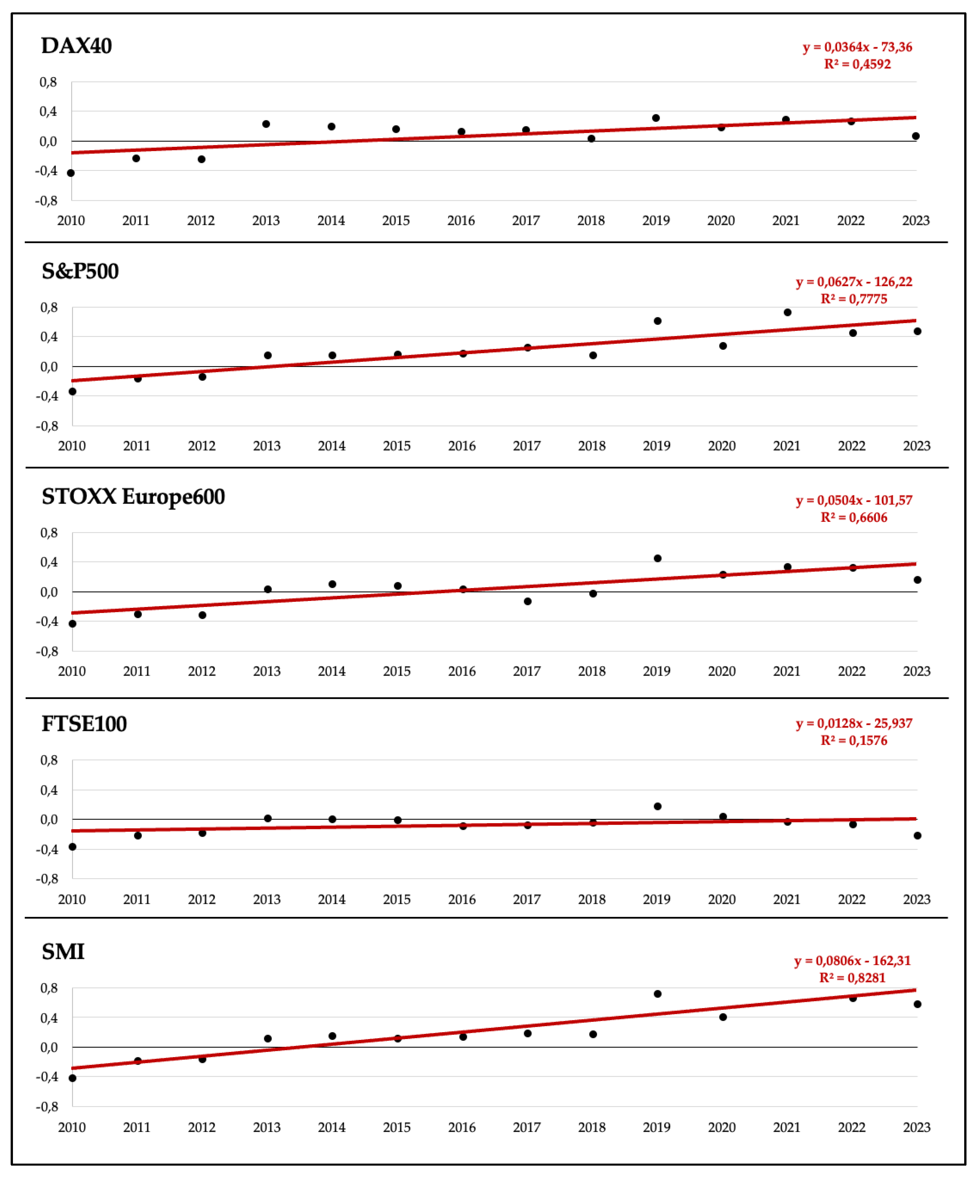
Linear regression analysis reveals positive growth in lambda factors across all indices between 2010 and 2023, with annualized increases ranging from 1.28% (for FTSE100) to 8.06% (for SMI). However, two methodological limitations warrant attention. First, negative lambda values emerge for all indices during 2010–2012, presenting an interpretive challenge. Since lambda is defined as the ratio of market risk premium to volatility, negative lambda values arise when the numerator is negative – that is, when the ten-year geometric mean market return is negative despite positive risk-free interest rates. Under the risk-return theory, negative market risk premiums are economically implausible. For example, the DAX40 in 2010 exhibited a ten-year geometric mean return of –4.75%, with a contemporaneous ten-year German government bond yield of 2.78%, yielding an implied market risk premium of –7.53%. With annualized volatility of 17.58, this produces a negative lambda factor, which contradicts fundamental financial theory stipulating positive risk compensation. Accordingly, removing observations with negative lambda factors due to their lack of being theoretically plausible, the following adjustment lines result:

Table 7.
Regression line for positive lambda factors.
| Index | Slope of Regression line |
| DAX40 | 0.0008x |
| S&P500 | 0.0467x |
| STOXX Europe600 | 0.0268x |
| FTSE100 | 0.0132x |
| SMI | 0.0699x |
Excluding negative lambda values yields significantly weaker upward trends in lambda factors. Given lambda’s sensitivity to the market return interval specification, a formal sensitivity analysis is necessary to establish the robustness of trend conclusions.
The sensitivity analysis systematically varies the market return interval from ten to 15 years, evaluating lambda factor sensitivity to this methodological choice.
Figure 14 plots regression slope coefficients as functions of interval length. Across all indices, a strong negative relationship exists: Lambda factors average 0.042 for ten-year intervals, decline to approximately 0.021 for 14-year intervals, and approach 0.001 for fifteen-year intervals (Pearson correlation = –0.9037, indicating strong negative dependency). Thus, the sensitivity analysis reveals that empirical conclusions regarding lambda factor trends depend critically on the length of the return interval.
Discussion in the context of the research question. Lambda factor trends are methodologically sensitive: fifteen-year intervals yield flat trends versus growth with ten-year intervals (Pearson correlation = -0.9037). This dependence precludes robust conclusions about risk aversion. Consequently, hypothesis H3 cannot be falsified based on quantitative evidence alone.
4.4. H4: Earnings Risk: EBIT Volatility
In line with the previous analyses, linear regression of distributional statistics investigates median, standard deviation and number of outliers. The analysis spans from 2006 to 2021 due to data availability constraints for DAX40 companies prior to 2006. The median CV exhibits a negative trend of –0.0053, indicating declining central tendency of earnings volatility over 15 years. This negative slope is driven predominantly by the 2011–2019 period. However, median CV values increased during 2020–2021, reaching levels observed during the 2008–2010 financial crisis, suggesting cyclical earnings volatility patterns.
Figure 15.
Development of selected CV-parameters.
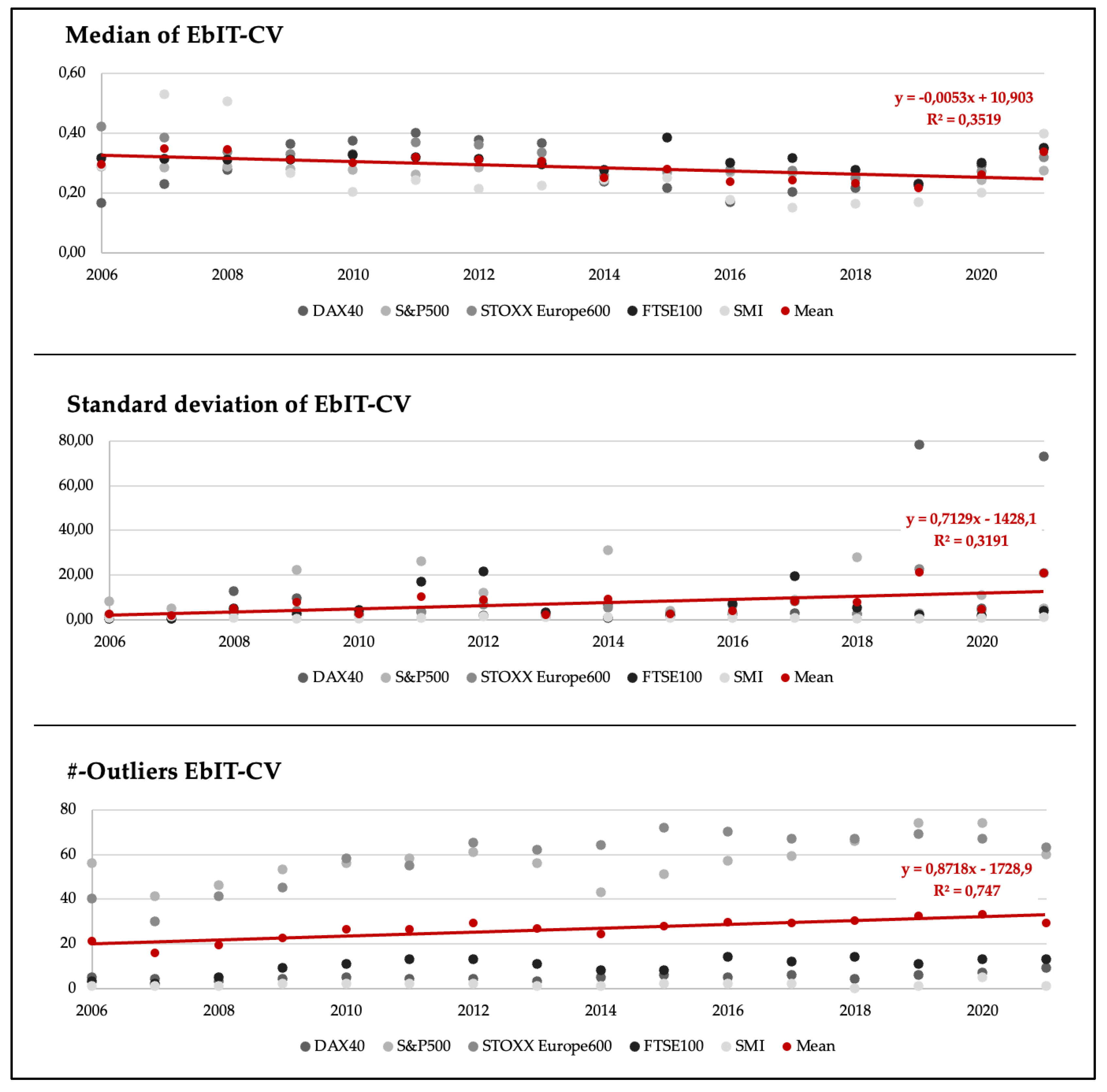
Standard deviation of CV (slope = 0.719) and outlier frequency (slope = 0.8718) are driven by two extreme values (78.33 in 2019, 72.76 in 2021). Excluding these reduces the standard deviation slope to 0.194, confirming median CV as the robust measure. This supports declining earnings volatility trends. Return-VaR and -CVaR are estimated across three methodological approaches: historical simulation, variance-covariance, and Monte Carlo methods. The analyses result in 6,588 slopes for the shortfall measures’ regression lines capturing the temporal trend in return-(C)VaR (see Figure 16).
Positive regression slopes indicate increasing return-(C)VaR implying that companies have risen EBIT margins in downside scenarios (worst 5% of cases) over time and consequently improved financial performance, even under adverse conditions.
In total 68.6% of regression slopes are positive, suggesting that in the majority of cases, return-(C)VaR measures demonstrate upward trends. This pattern corroborates the median CV finding namely that earnings volatility has generally declined, contradicting any claim of increased earnings risk.
Figure 17 presents return-CVaR statistics across all five indices over the 2004–2021 period. The median return-CVaR increased significantly, rising from 0.5% in 2004 to 5.0% in 2021 – a tenfold increase reflecting improved downside earnings performance. Since higher return-CVaR thresholds indicate that worst-case EBIT scenarios have improved, this pattern signals reduced earnings risks. However, the IQR expanded 71.6% over the same period. This noticeable contradiction resolves upon examination: the IQR expansion reflects rightward distribution shift rather than tail-risk deterioration. Specifically, the 75th percentile return-CVaR quantile increased due to higher average return-CVaR values across firms, not due to emergence of negative outliers or distribution deterioration.
Discussion in the context of the research question. Multiple analytical approaches confirm no systematic increase in earnings risk. Median CV declined, negative EBIT frequencies diminished, and 68.6% of return-(C)VaR regression slopes were positive, indicating improved downside performance across all methods. Thus, hypothesis H4 is falsified: observable earnings risk metrics provide no explanation for the WACC phenomenon.
4.5. H5: Financial Structure Risk: Debt Ratio Analyses
Financial structure risk is measured by debt ratios calculated on both book-value and market-value bases. DAX40 companies maintained relatively stable leverage ratios throughout the study period, with average debt ratios ranging from 57.9% and 74.0% (book values) and 48.7% and 67.0% (market values) across 2004–2021. Notably, both measures exhibit downward trends. These declines indicate reduced financial leverage and consequently diminished financial structure risk for DAX40 companies.
Figure 18.
Debt ratios of DAX40 companies.
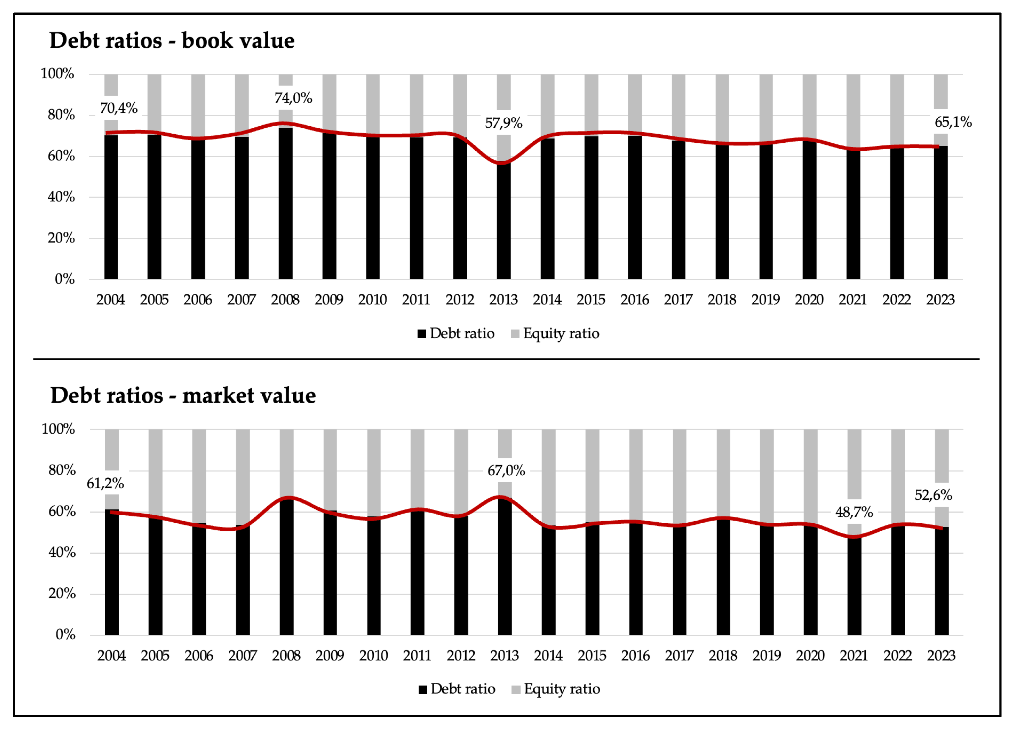
Discussion in the context of the research question. Empirical analysis of debt ratios across the 2004–2021 period provides falsification of hypothesis H5. Both book-value and market-value leverage metrics demonstrate substantial declines, indicating reduced financial structure risk over the study period. Consequently, changes in financial leverage cannot explain observed WACC persistence.
5. Conclusions & Outlook
Systematic evaluation of five risk dimensions reveals no support for explanations of WACC persistence based on observable risk parameters. The following key statements summarize the findings:
- ▪ H1 – Systematic risk: Beta factor variance declined 41.5% and IQR compression reached 72.1%, indicating reduced systematic risk. Hypothesis H1 is falsified.
- ▪ H2 – Overall market risk: Median and IQR exhibit negative trend slopes, with volatility buffers positive in 69.7% of cases. Upside opportunity exceeds shortfall risk by 16.5% at 50% probability. Hypothesis H2 is falsified. This evidence collectively demonstrates declining market risk exposure, falsifying hypothesis H2.
- ▪ H3 – Market price of risk (lambda factors): Lambda factor trends are methodologically sensitive (Pearson correlation = -0.9037), with 15-year intervals yielding flat trends. Hypothesis H3 cannot be falsified. Thus, hypothesis H3 cannot be accepted or rejected based on empirical evidence alone, indicating increased investor risk aversion does not provide robust explanation for WACC persistence.
- ▪ H4 – Firm-specific earnings risk (EBIT volatility): Median CV declined (slope = -0.0053) and 68.6% of return-(C)VaR regression slopes were positive, indicating reduced earnings volatility. Hypothesis H4 is falsified: earnings risk demonstrates no systematic increase.
- ▪ H5 – Financial structure risk (debt ratios): Book-value debt ratios declined 7.53 percentage points and market-value leverage fell 14.05 percentage points (2004 baseline), indicating reduced capital structure risk. Hypothesis H5 is falsified. Consequently, hypothesis H5 is falsified: observable changes in financial leverage do not account for reported WACC stability.
The falsification of four out of five hypotheses, H3) indicate a fundamental disconnect between theoretically consistent WACC calculations based on observable market and fundamental parameters and practitioner applications in value-based management. These results imply that factors beyond conventional quantitative risk metrics drive corporate WACC reporting practices.
Quantitative risk analyses reach explanatory limits: standard market and fundamental data cannot account for observed WACC estimation behavior. Complementary qualitative research employing problem-centered, semi-structured expert interviews analyzed through grounded theory methods constitutes the next phase of this research endeavor. The investigation reveals that behavioral economics (risk aversion, opportunism, subjectivity), organizational constraints (strategic path dependency, implementation complexity, financial criterion rigidity), and model-theoretic discretion (parameter averaging, analyst influence, supplementary risk adjustments) substantially shape practical WACC determination – factors that quantitative risk analysis cannot capture. These results are being discussed in detail in part II of this article series.
Abbreviations
The following abbreviations are used in this manuscript:
| BR | Volatility Buffer Ratio |
| CAPM | Capital Asset Pricing Model |
| CV | Coefficient of Variance |
| CVaR | Conditional Value at Risk |
| EBIT | Earnings Before Interests and Taxes |
| IQR | Interquartile Range |
| KDE | Kernel Density Estimation |
| MC | Monte Carlo Method |
| nBR | Negative Volatility Buffer Ratio |
| NPV | Net Present Value |
| pBR | Positive Volatility Buffer Ratio |
| RIC | Refinitiv Instruments Code |
| VaR | Value at Risk |
| WACC | Weighted Average Cost of Capital |
References
- Albrecht, P./Maurer, R. (2016). Investment- und Risikomanagement: Modelle, Methoden, Anwendungen. Schäffer-Poeschel Verlag Stuttgart.
- Ang, R./Hodrick, R. J./Xing, Y./Zhang, X. (2006). The Cross-Section of Volatility and Expected Returns. The Journal of Finance, 61(1), p. 259–299.
- Auer, B. R./Rottmann, H. (2010). Statistik und Ökonometrie für Wirtschaftswissenschaftler: Eine anwendungsorientierte Einführung. Gabler.
- Banque centrale du Luxembourg (2024a). Entwicklung der Rendite zehnjähriger Staatsanleihen der USA in den Jahren von 1995 bis 2023 (Graph). Available online: https://de.statista.com/statistik/daten/studie/383112/umfrage/entwicklung-der-rendite-zehnjaehriger-staatsanleihen-der-usa/ (accessed on 25. 09. 2024).
- Banque centrale du Luxembourg (2024b). Entwicklung der Rendite zehnjähriger Staatsanleihen Deutschlands in den Jahren von 1995 bis 2023 (Graph). Available online: https://de.statista.com/statistik/daten/studie/200193/umfrage/entwicklung-der-rendite-zehnjaehriger-staatsanleihen-in-deutschland/ (accessed on 25. 09. 2024).
- Bansal, R./Kiku, D./Ivan, S./Yaron, A. (2012). Volatility, the macroeconomy and asset prices. NBER Working Paper Series.
- Bertram, I./Castedello, M./Tschöpel, A. (2015). Überlegungen zur Marktrendite und zur Marktrisikoprämie. Corporate Finance, 12, p. 468–473.
- Bilinski, P./Lyssimachou, D. (2014). Risk Interpretation of the CAPM ‘s Beta: Evidence from a New Research Method, Abacus, 50(2), p. 203–226.
- Brotherson, T. W./Eades, K. M./Harris, R. S./Higgins, R. C. (2013). “Best Practices” in Estimating the Cost of Capital: An Update. Journal of Applied Finance, 23(1), p. 1–19.
- Carhart, M. M. (1997), On Persistence in Mutual Fund Performance. The Journal of Finance, 52(1), p. 57–82.
- Damodaran, A. (2022). Equity Risk Premiums (ERP): Determinants, Estimation and Implications – The 2022 Edition. Updated: March 2022, Stern School of Business.
- Diether, K. B./Malloy, C. J./Scherbina, A. (2002). Differences of Opinion and the Cross Section of Stock Returns. The Journal of Finance, 57(5), p. 2113–2141.
- Dreger, C./Kosfeld, R./Eckey, H.-F. (2014). Ökonometrie und empirische Wirtschaftsforschung. Springer.
- Dumas, B./Solnik, B. (1995). The World Price of Foreign Exchange Risk. The Journal of Finance, 50(2), p. 445–479.
- Efron, B./Tibshirani, R. J. (1994). An Introduction to the Bootstrap. Chapman and Hall/CRC.
- Enzinger, A./Kofler, P. (2011). DCF-Verfahren: Anpassung der Beta-Faktoren zur Erzielung konsistenter Bewertungsergebnisse. RWZ, 2, p. 52–57.
- Fama, E. F./French, K. R. (1992), The Cross-Section of Expected Stock Returns. The Journal of Finance, 47(2), p. 427–465.
- Farooq, U./Ahmed, J./Khan, S. (2021). Do the macroeconomic factors influence the firm’s investment decisions? A generalized method of moments (GMM) approach. International Journal of Finance & Economics, 26(1), p. 790–801.
- Frank, M. Z./Shen, T. (2016). Investment and the weighted average cost of capital. Journal of Financial Economics, 119(2), p. 300–315.
- Franzen, D./Schäfer, K. (2018). Assetmanagement. Portfoliobewertung, Investmentstrategien und Risikoanalyse. Schäffer-Poeschel Verlag Stuttgart.
- Gehrke, M. (2022). Angewandte empirische Methoden in Finance & Accounting. Umsetzung mit R. DeGruyter Oldenburg.
- Gleißner, W. (2014). Kapitalmarktorientierte Unternehmensbewertung: Erkenntnisse der empirischen Kapitalmarktforschung und alternative Bewertungsmethoden. Corporate Finance, 4, p. 151–167.
- Gleißner, W. (2016). Unternehmenswert, Ertragsrisiko, Kapitalkosten und fundamentales Beta - Studie zu DAX und MDAX. BewertungsPraktiker, 2, p. 60–70.
- Good, P. (2000). Permutation Tests: A Practical Guide to Resampling methods for Testing Hypotheses. Springer.
- Hall, P. (1992). The Bootstrap and Edgeworth Expansion. Springer.
- Horowitz, J. L. (2001). The Bootstrap. In Heckman, J. J./Leamer, E. E. (Ed.), Handbook of econometrics. p. 3160–3223.
- Johnson, T. C. (2004). Forecast Dispersion and the Cross Section of Expected Returns. The Journal of Finance, 59(5), p. 1957–1978.
- Klandt, H./Heidenreich, S. (2017). Empirische Forschungsmethoden in der Betriebswirtschaftslehre. DeGruyter Oldenburg.
- Larson, C. R./Resutek, R. J. (2017). Types of investor uncertainty and the cost of equity capital. Journal of Business Finance & Accounting, 44(9-10), p. 1169–1193.
- Lehmann, K. (2019). Wirkungslose EZB-Medizin - Kapitalkosten immun gegen Nullzins. Available online: https://mpra.ub.uni-muenchen.de/104332/ (accessed on 21.10.2025).
- London Stock Exchange (2023). FTSE 100. Available online: https://www.londonstockexchange.com/indices/ftse-100/constituents/table, (accessed on 16.05.2023).
- MacKinnon/James G. (2007). Bootstrap Hypothesis Testing. Available online: https://www.econstor.eu/bitstream/10419/189403/1/qed_wp_1127.pdf (accessed on 22.10.2025).
- Merton, R. C. (1973). An Intertemporal Capital Asset Pricing Model. Econometrica, 41(5), S. 867–887.
- Poterba, J. M./Summers, L. H. (1995). A CEO Survey of U.S. Companies Time Horizons and Hurdle Rates. Sloan Management Review, 37(1), p. 43–53.
- Roy, A. D. (1952). Safety First and the Holding of Assets. Econometrica, 20(3), p. 431–449.
- Pratt, S. P./Grabowski, R. J. (2014). Cost of Capital: Applications and Examples. 5. Ed., Hoboken, New Jersey.
- Saleheen, J./Levina, I./Melolinna, M./Tatomir, S. (2017). The financial system and productive investment: new survey evidence. Bank of England Quarterly Bulletin, 57(1), p. 4–17.
- Santis, G. de/Gerard, B. (1997), International Asset Pricing and Portfolio Diversification with.
- Time-Varying Risk. The Journal of Finance, 52(5), p. 1881–1912.
- Six (2023). Indexzusammensetzung des SMI. Available online: https://www.six-group.com/en/products-services/the-swiss-stock-exchange/market-data/indices/equity-indices/smi.html (accessed on 16.05.2023).
- Statistics Denmark (2024). Entwicklung der Rendite zehnjähriger Staatsanleihen des Vereinigten Königreichs in den Jahren von 1989 bis 2023 (Graph). Available online: https://de.statista.com/statistik/daten/studie/572240/umfrage/entwicklung-der-rendite-zehnjaehriger-staatsanleihen-des-vereinigten-koenigreichs/ (accessed on 25.09.2024).
- Steiner, M./Bruns, C./Stöckl, S. (2017). Wertpapiermanagement: Professionelle Wertpapieranalyse und Portfoliostrukturierung. Schäffer-Poeschel Verlag Stuttgart.
- Stoxx (2023). List of STOXX Europe600 companies. Available online: https://www.stoxx.com/document/Bookmarks/CurrentComponents/SXXGR.pdf (accessed on 16.05.2023).
- Wikimedia Foundation, Inc. (2023). List of S&P 500 companies. Available online: https://en.wikipedia.org/wiki/List_of_S%26P_500_companies (accessed on 05.04.2023).
- Wikimedia Foundation, Inc. (2024). DAX. Available online: https://de.wikipedia.org/wiki/DAX (accessed on 12.09.2024).
Figure 1.
Development of WACC and risk-free interest rate.
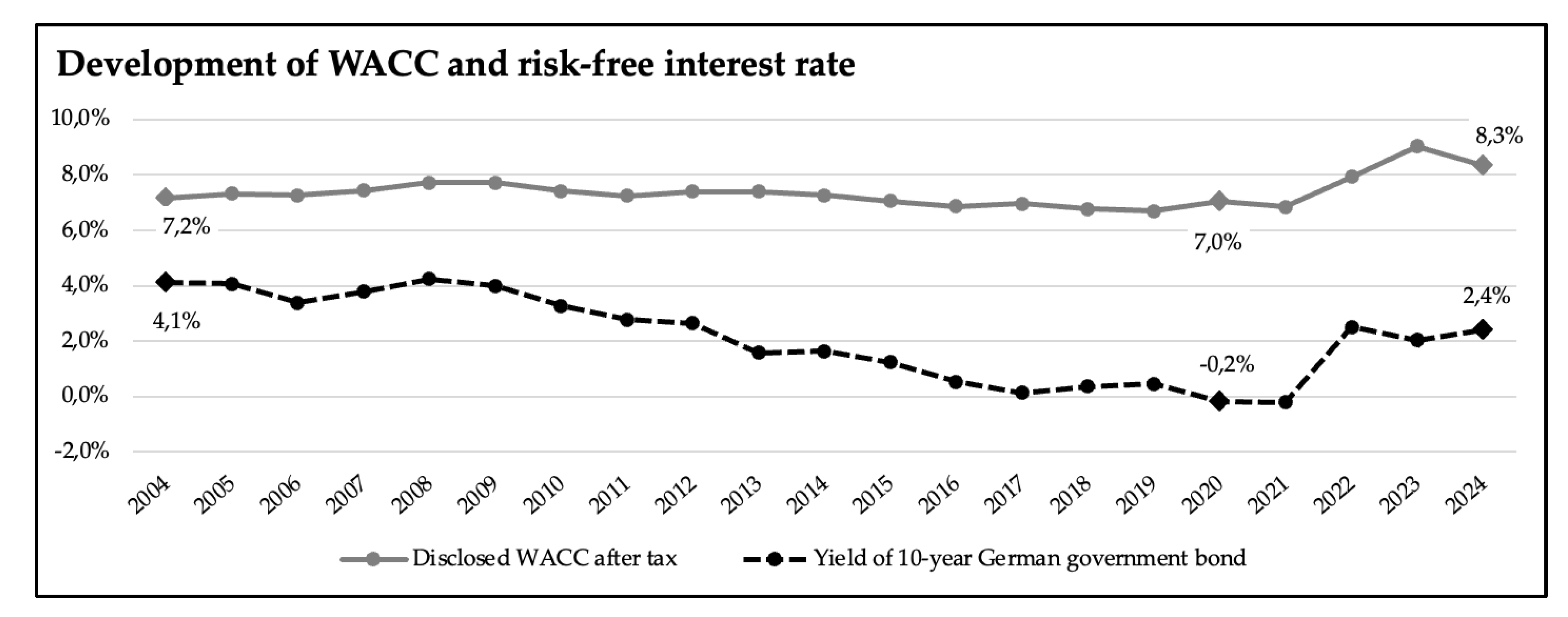
Figure 2.
WACC as the sum of risk-free and risky components.
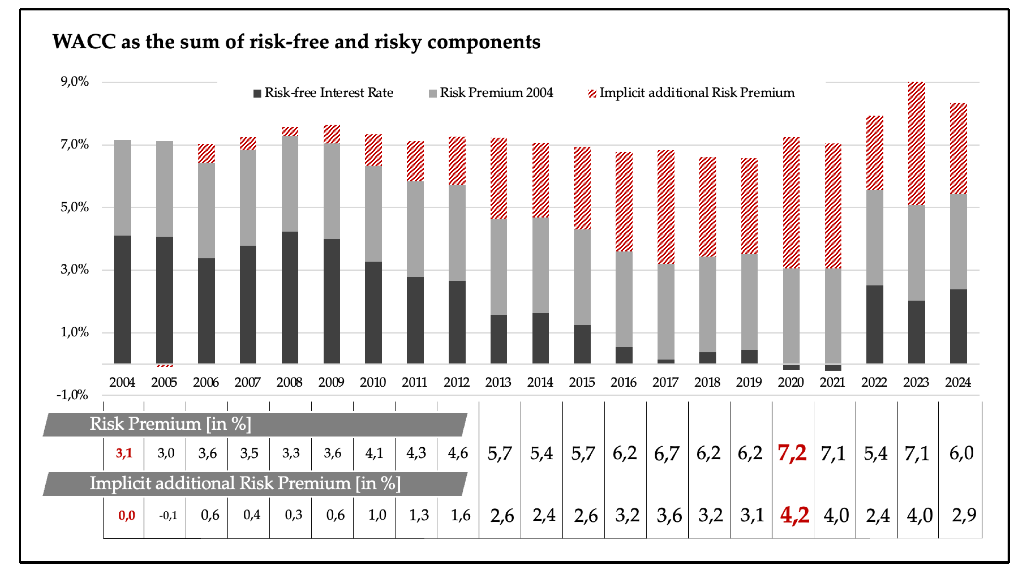
Figure 3.
Bootstrap method.
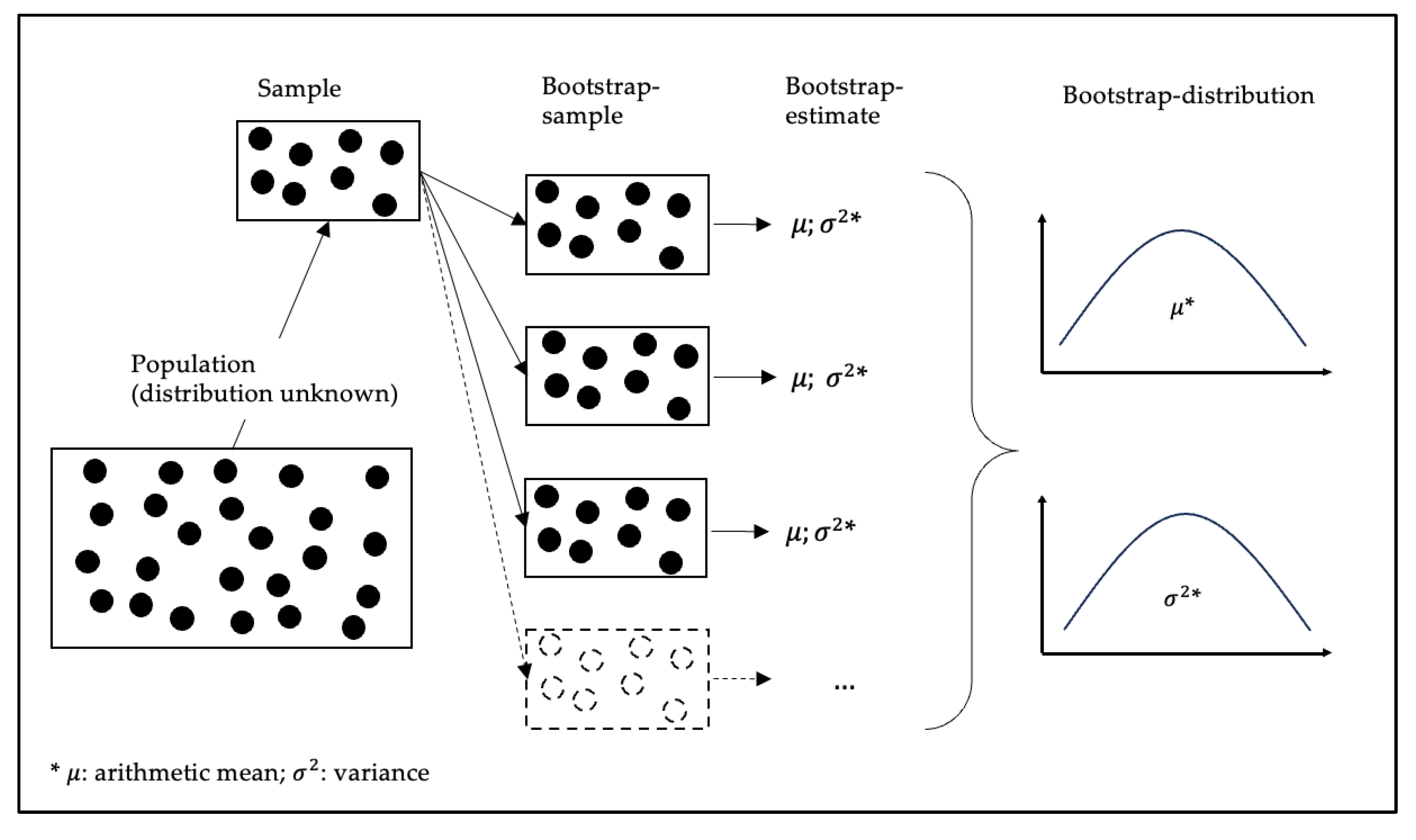
Figure 4.
Conceptual depiction of analyzing historical volatilities as estimators for expected value.
Figure 4.
Conceptual depiction of analyzing historical volatilities as estimators for expected value.
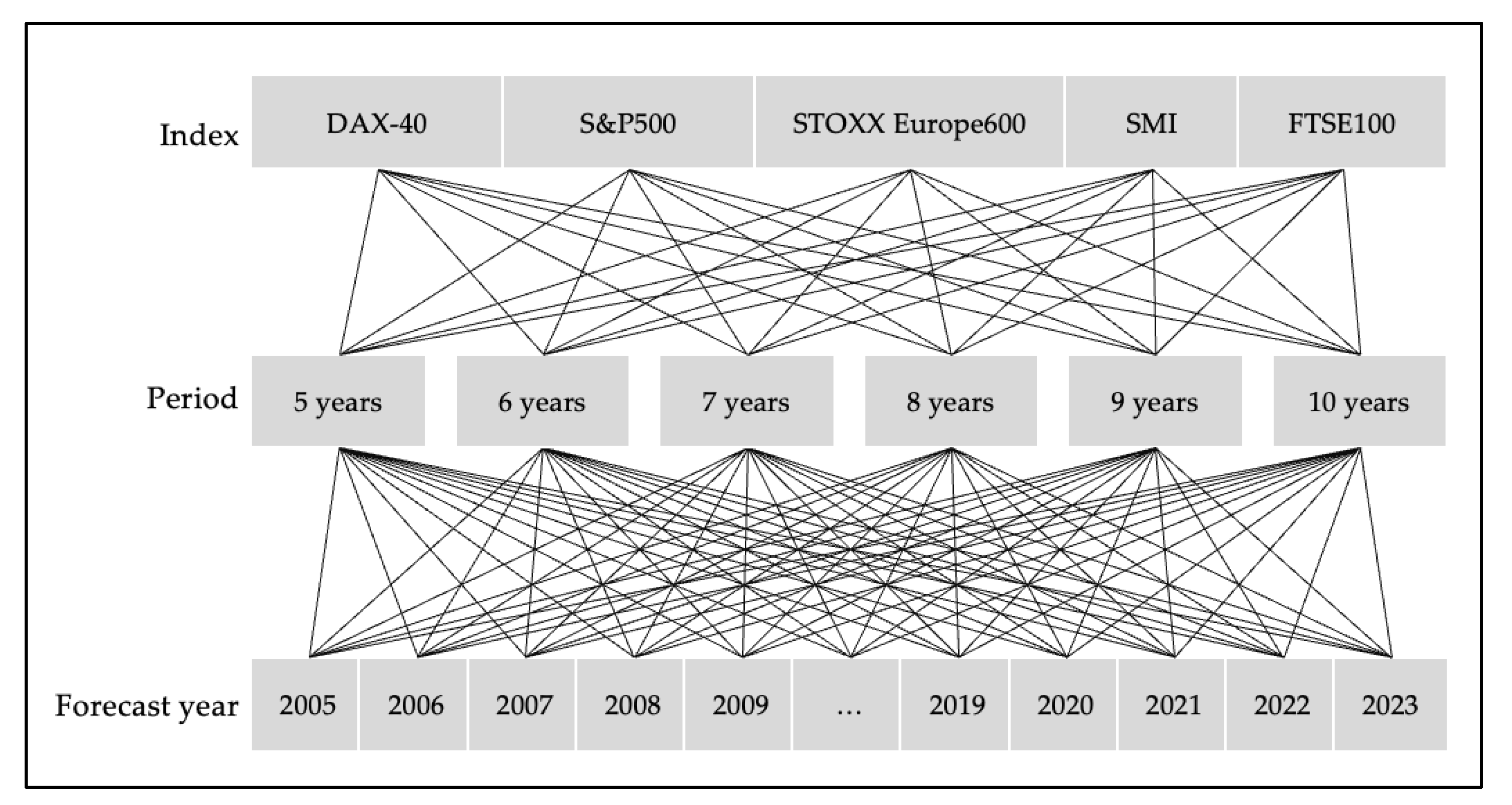
Figure 5.
Difference of mean and median plus Interquartile range of all indices.
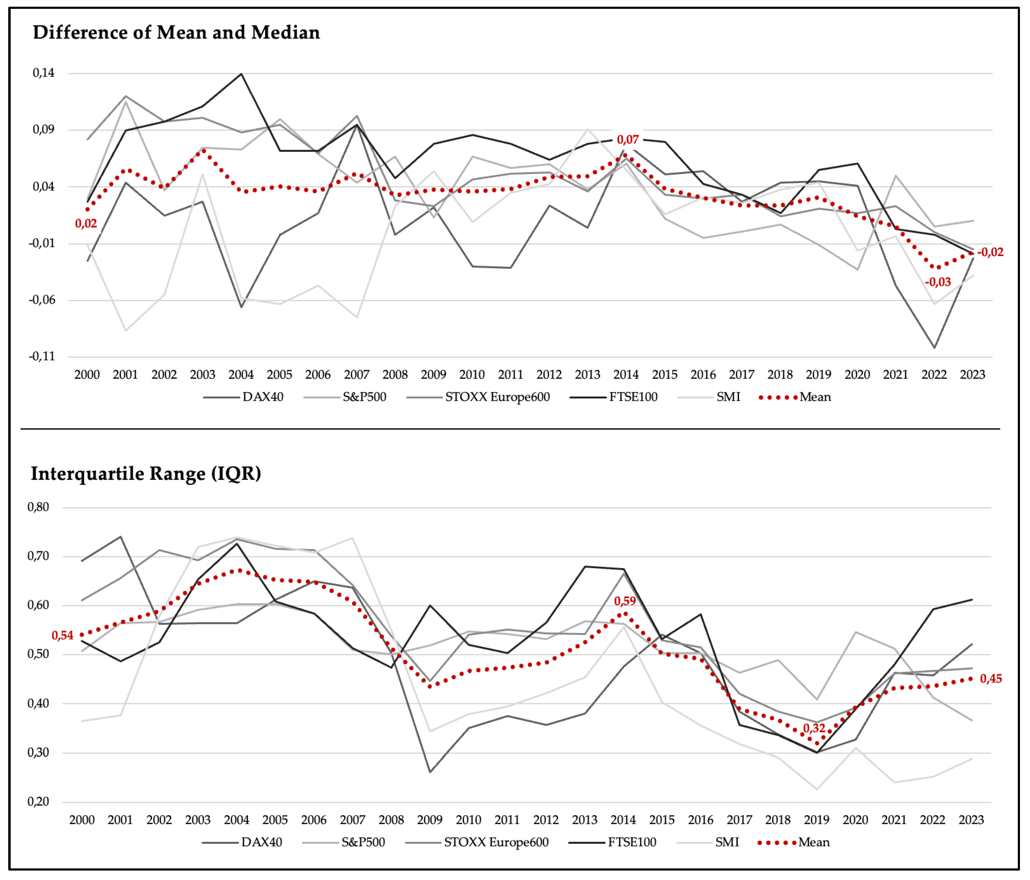
Figure 6.
Distribution of Bootstrap-variance of DAX40 Beta factors (Python screenshot).
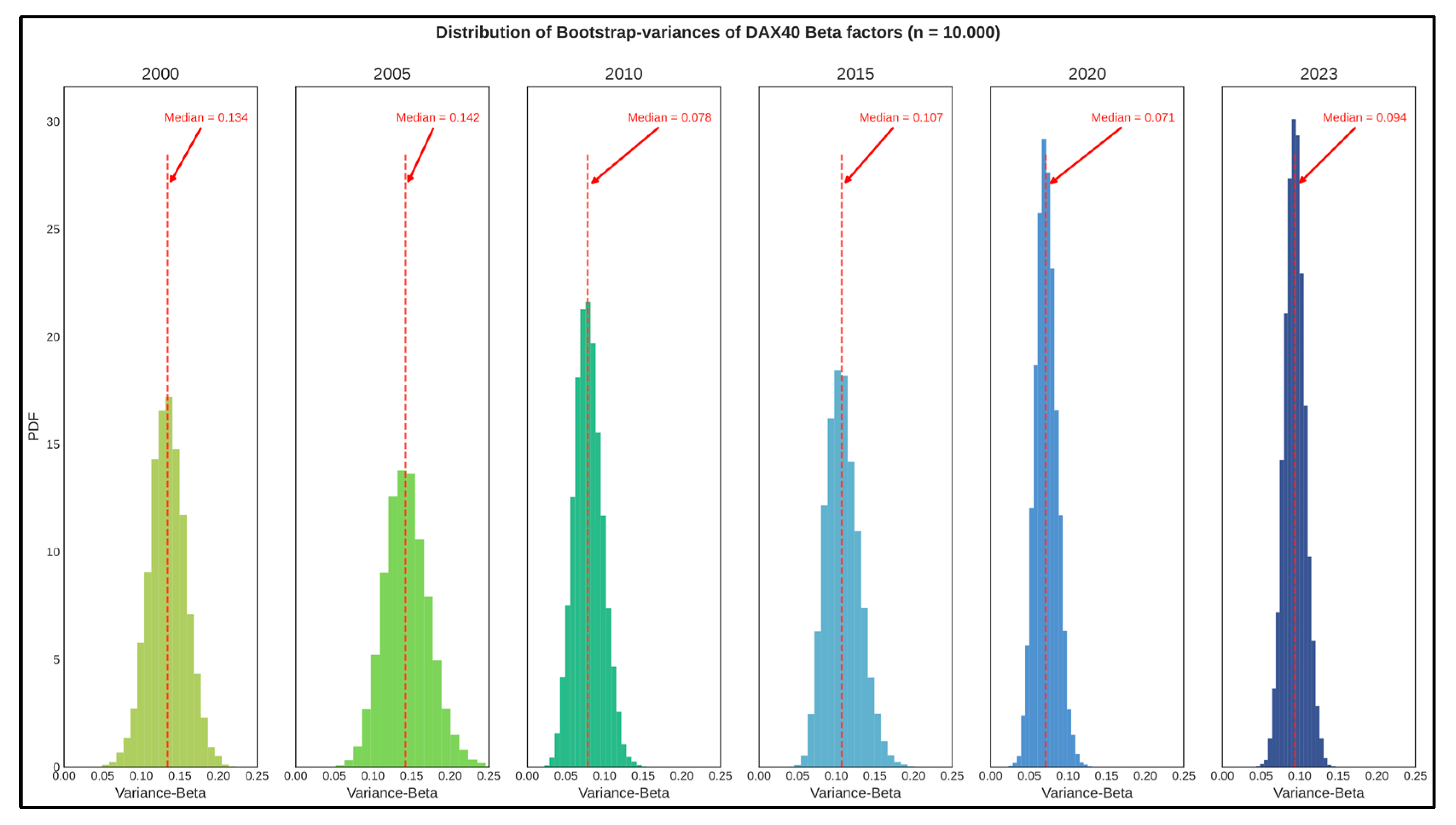
Figure 7.
Median of Bootstrap variances.
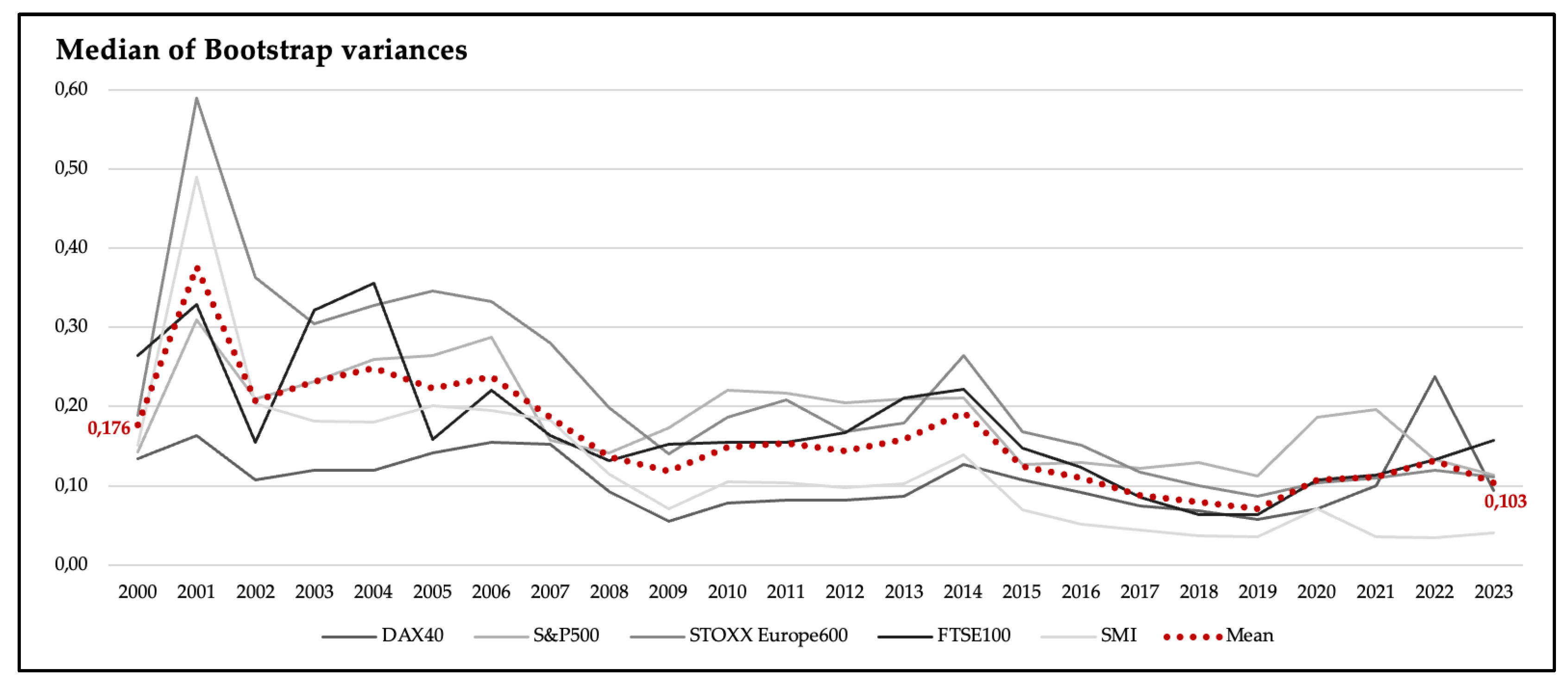
Figure 8.
Confidence interval widths of Bootstrap variances.
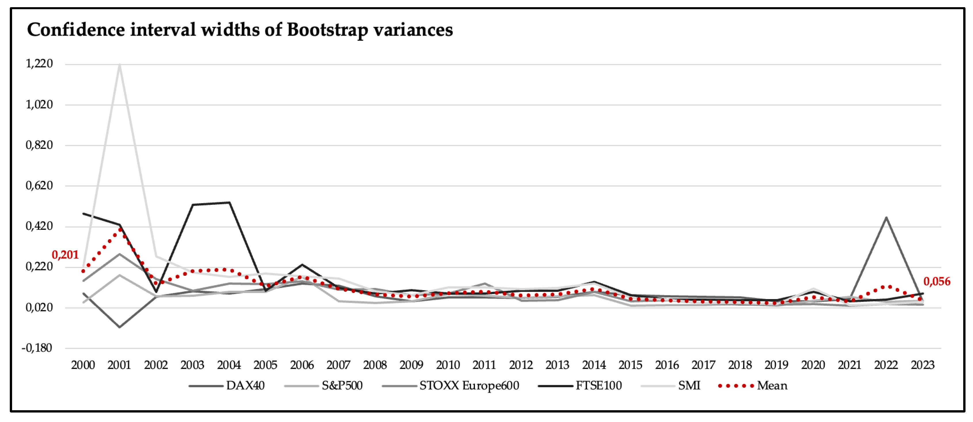
Figure 9.
Coefficients and variances of unlevered beta factors.
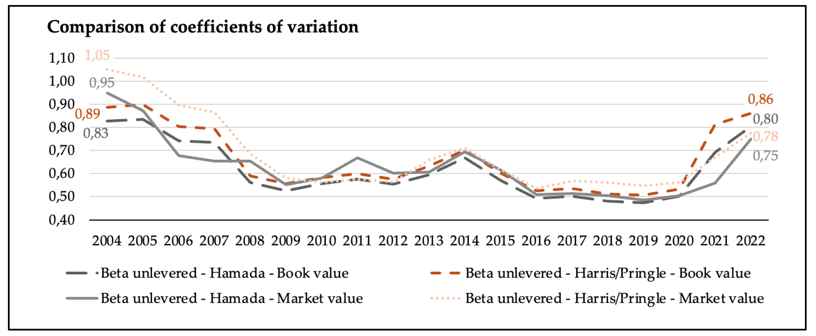
Figure 10.
Boxplots of volatility across indices (Python screenshot).
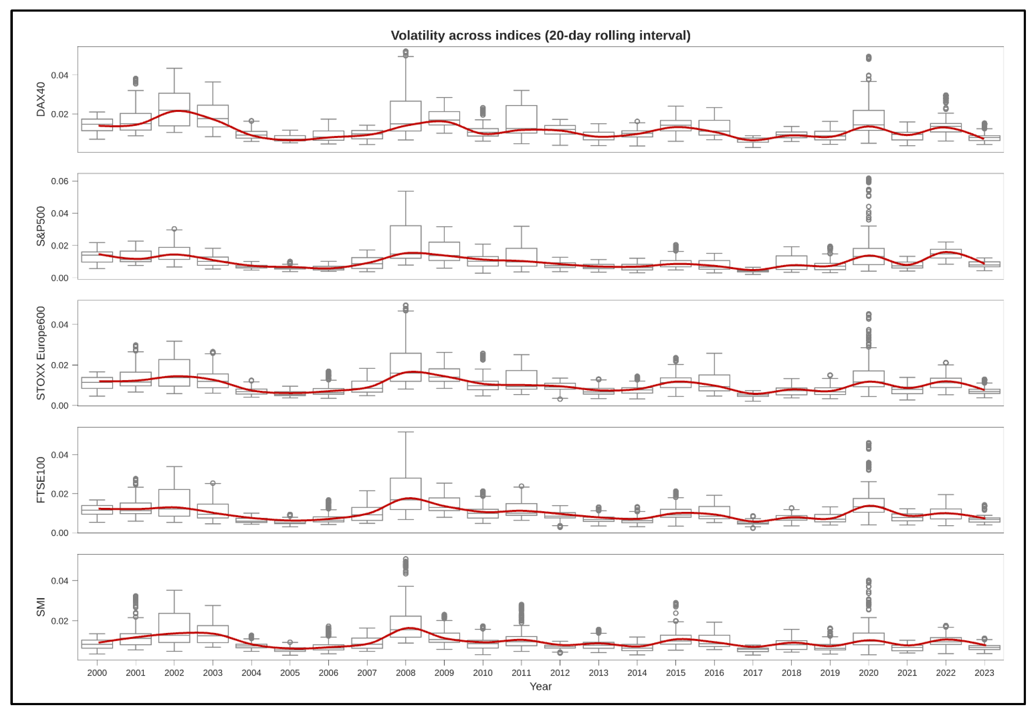
Figure 11.
Volatility buffer.
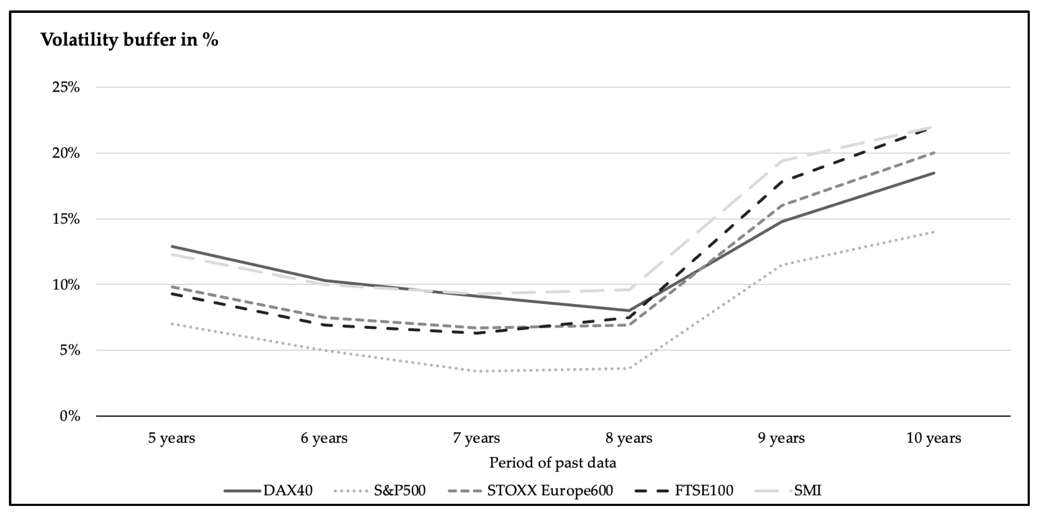
Figure 12.
Positive and negative Volatility buffer ratios and its probability of occurrences.
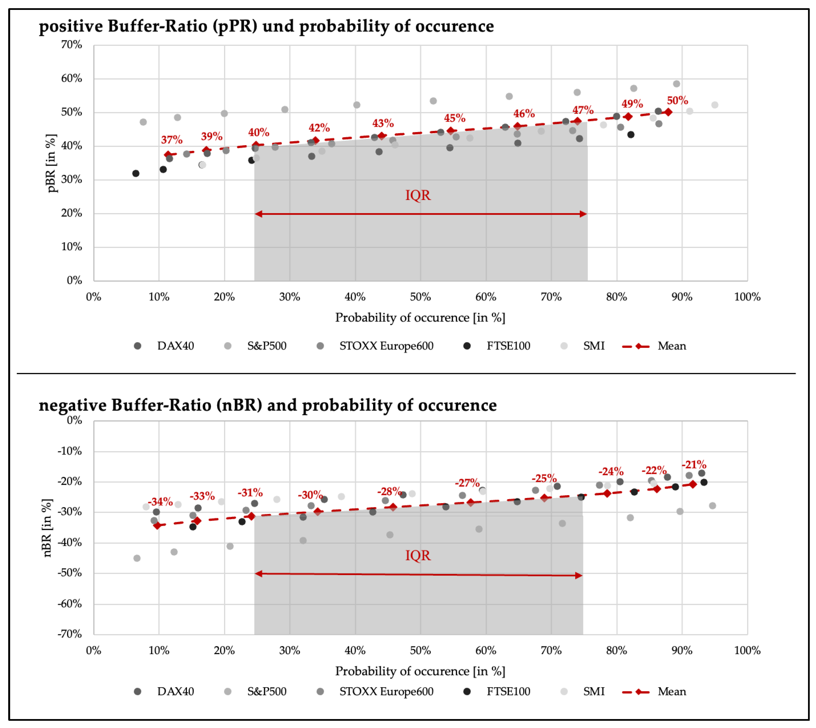
Figure 14.
ensitivity analysis of lambda factors.
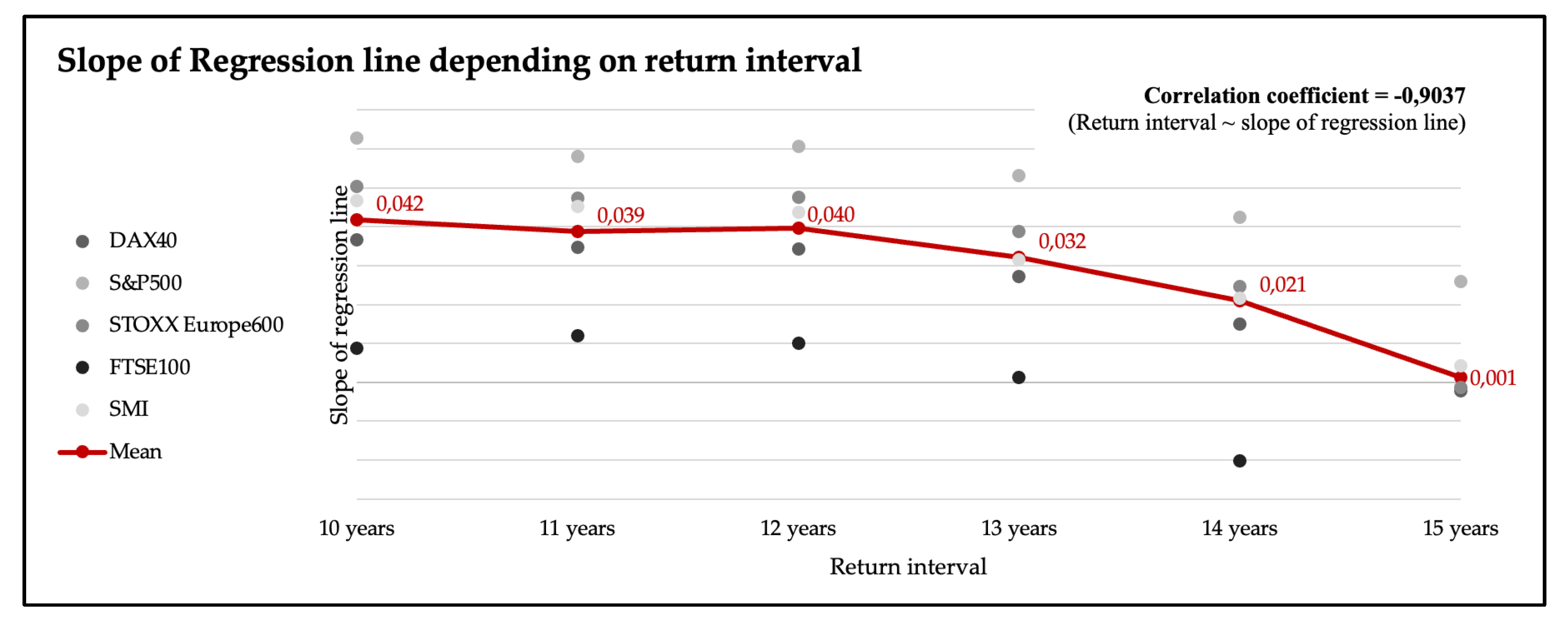
Figure 16.
Slope of Regression lines of (C)VaR-Methods.
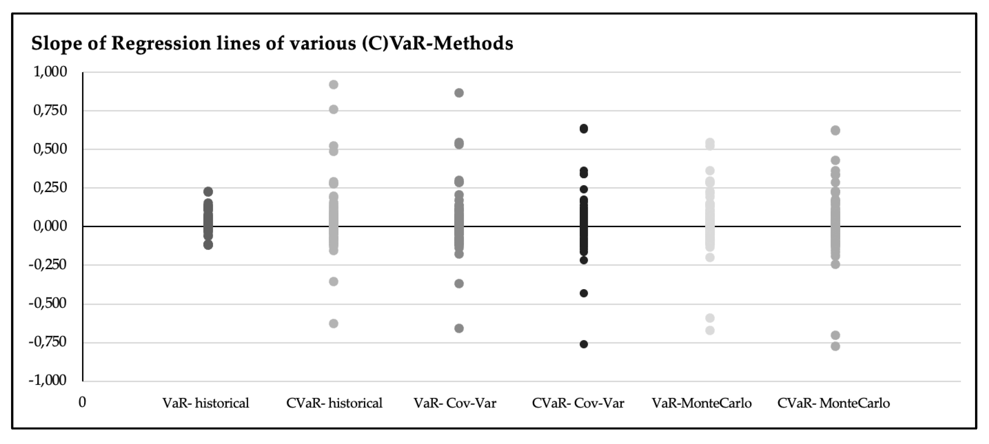
Figure 17.
Selected statistics of CVaR.
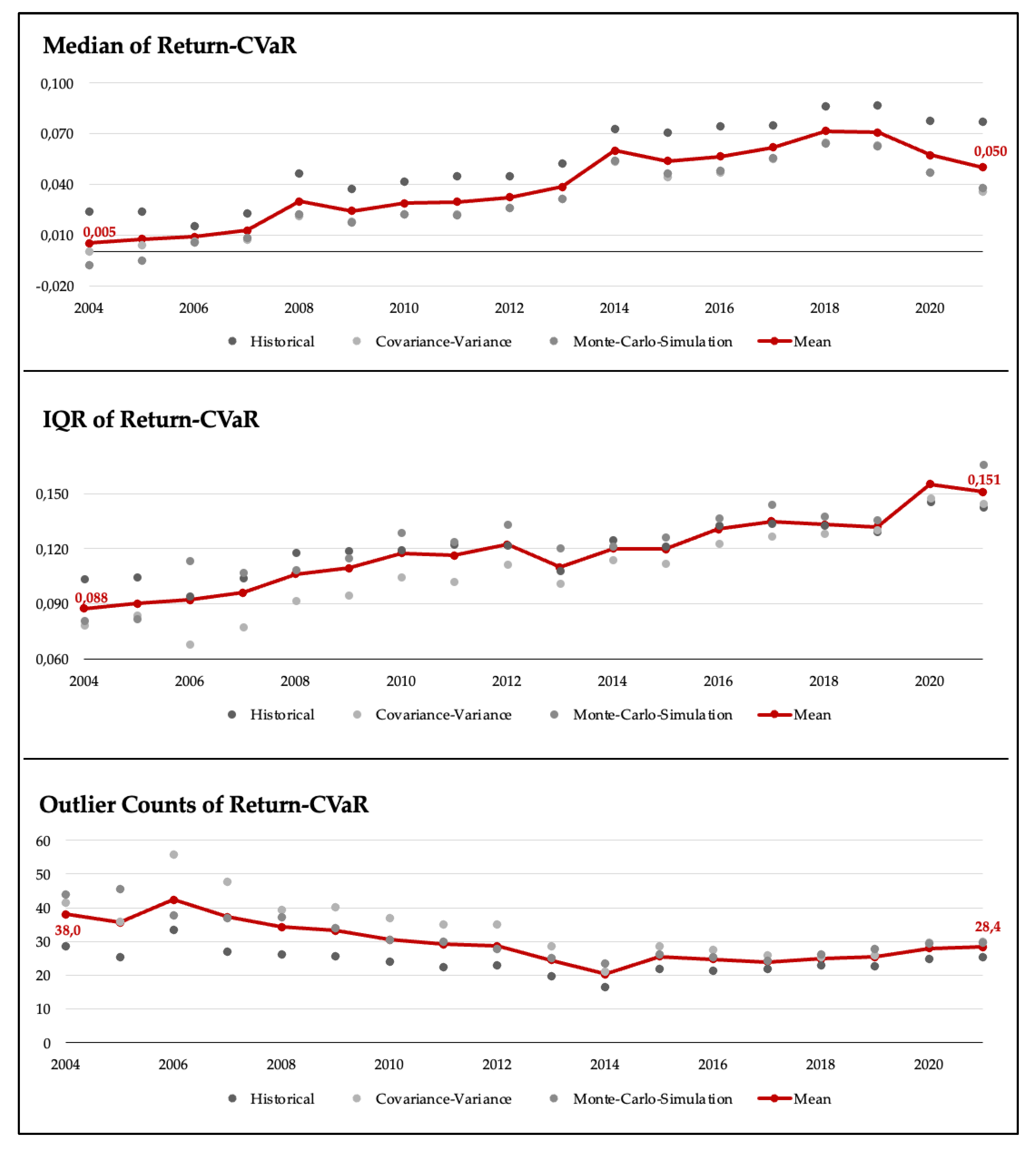
Table 1.
Indices, RIC and data sources.
| Index | RIC | Retrieval date | Institution |
| DAX40 | GDAXI | 20.03.2023 | Wikimedia (2024) |
| S&P500 | GSPC | 04.05.2023 | Wikimedia (2023) |
| STOXX Europe600 | SXXP | 16.05.2023 | Stoxx (2023) |
| FTSE100 | FTSE | 16.05.2023 | London Stock Exchange (2023) |
| SMI | SSMI | 16.05.2023 | SIX Swiss Exchange (2023) |
Table 4.
Proxies used for risk-free interest rate.
| Index | Proxy for Risk-Free Interest Rate |
| DAX40 price index | Yield on a ten-year German governement bond |
| S&P500 | Yield on a ten-year US governement bond |
| STOXX Europe600 | Yield on a ten-year German governement bond |
| FTSE100 | Yield on a ten-year UK governement bond |
| SMI | Yield on long-term bonds in Switzerland |
Table 5.
Regression analysis of test statistics je index.
| Index | Parameter | Slope of regression line | Coefficient of determination |
| DAX40 | Median | -0.00022 | 0.166 |
| IQR | -0.00022 | 0.134 | |
| #-Outliers | 0.35 | 0.108 | |
| S&P500 | Median | -0.00011 | 0.056 |
| IQR | -7*10-5 | 0.013 | |
| #-Outliers | 0.167 | 0.014 | |
| STOXX Europe600 | Median | -0.00012 | 0.089 |
| IQR | -0.00015 | 0.105 | |
| #-Outliers | 0.248 | 0.031 | |
| FTSE100 | Median | -0.0001 | 0.063 |
| IQR | -0.00015 | 0.09 | |
| #-Outliers | 0.327 | 0.056 | |
| SMI | Median | -0.00012 | 0.127 |
| IQR | -0.00016 | 0.143 | |
| #-Outliers | -0.067 | 0.002 |
Table 6.
Share of positive volatility buffer.
| Index | Interval (in years) | |||||
| 5 | 6 | 7 | 8 | 9 | 10 | |
| DAX40 | 68% | 61% | 71% | 69% | 67% | 71% |
| S&P500 | 74% | 67% | 65% | 62% | 67% | 79% |
| STOXX Europe600 | 68% | 61% | 65% | 69% | 73% | 71% |
| FTSE100 | 68% | 72% | 76% | 69% | 73% | 79% |
| SMI | 68% | 56% | 71% | 69% | 80% | 79% |
Disclaimer/Publisher’s Note: The statements, opinions and data contained in all publications are solely those of the individual author(s) and contributor(s) and not of MDPI and/or the editor(s). MDPI and/or the editor(s) disclaim responsibility for any injury to people or property resulting from any ideas, methods, instructions or products referred to in the content. |
© 2026 by the authors. Licensee MDPI, Basel, Switzerland. This article is an open access article distributed under the terms and conditions of the Creative Commons Attribution (CC BY) license (http://creativecommons.org/licenses/by/4.0/).
Copyright: This open access article is published under a Creative Commons CC BY 4.0 license, which permit the free download, distribution, and reuse, provided that the author and preprint are cited in any reuse.


