

Submitted:
05 February 2026
Posted:
09 February 2026
You are already at the latest version
Abstract
This paper aims to define the optimal microgrid topology for rural electrification based on the lowest total cost (TOTEX) by comparing LVAC and LVDC microgrids across three different scenarios. An LVAC radial topology is first designed using MILP for phase balancing and SP for connections, then implemented with a GA to allocate and size SHSs, forming an LVAC microgrid. Next, an LVDC topology is then derived from the LVAC structure and integrated with SHSs under three scenarios: (1) using the same SHS sizes, locations, and quantities as the LVAC microgrid; (2) using GA to re-determine SHS sizes and locations, forming an LVDC microgrid; and (3) clustering the LVDC topology into nano-grids, each defined by GA for SHS sizing and placement and connected to the main feeder via bi-directional converters. Finally, all LVAC and LVDC scenarios are simulated over a 30-year planning horizon for analysis. A non-electrified village located in Cambodia has been selected for a case study to validate the proposed methods. The results have been obtained and provide a comparison of performance indicators (i.e., costs, energy production, losses, CO₂ emissions, and autonomous energy) among the microgrids (LVAC and LVDC). Based on the TOTEX results, the LVAC microgrid is considered more economical than the LVDC microgrid in each scenario in this study.
Keywords:
LVAC and LVDC microgrids
; nano-grids
; rural electrification
; SHSs
; TOTEX
1. Introduction
Low-voltage (LV) microgrids are becoming of interest due to their capability to ensure a reliable power supply and improve overall system efficiency [1,2]. An LV microgrid is defined as a small-scale local power distribution system capable of operating in either isolated mode or in connection with the main grid [3,4]. It also provides a flexible and reliable approach for integrating distributed energy resources (DERs) such as photovoltaic (PV) systems, hydropower, wind turbines, and battery energy storage systems (BES) [5,6,7]. They deliver a reliable energy supply and a high level of sustainability, reducing environmental impacts compared with traditional energy sources such as fossil fuels or coal [4,5,8]. Traditionally, the LVAC microgrid has been the standard choice due to its compatibility with existing networks [9,10,11]. However, the increasing adoption of LVDC systems offers a compelling alternative, especially as more and more DERs generate, use and store power in DC form [8,12]. As the energy landscape evolves, comparing LVAC and LVDC microgrids becomes crucial to determine the most effective configurations for future power networks [9]. Each system has its own advantages and challenges: LVAC is widely understood and standardized [13], whereas LVDC offers potential efficiency gains by eliminating the need for power conversion in DC-dominated systems [9]. To date, in the context of LV microgrid planning, researchers and distribution system operators (DSOs) still face challenges in deciding whether to operate an LV microgrid network in AC or DC form to minimize TOTEX and enhance overall system efficiency [9]. Meanwhile, many existing studies have proposed methodologies for optimizing LV microgrid topology (including siting and sizing of DERs) in either AC or DC form, or by comparing both topologies based on various research objectives. Consequently, these works have been reviewed in the following literature.
Reference [14] proposes a method that focuses on the optimal design of an LV distribution system for rural electrification, aiming for the lowest total cost. Initially, a topology is defined based on the first-fit bin-packing (FFBP) and SP algorithms. Next, two iterative techniques and genetic algorithm (GA) are applied to determine the sizes and locations of PVs and DeBESs (decentralized BESs). This method is implemented in a non-electrified village as a test case. The study concludes that an LV system integrated with PVs and batteries is less expensive over a 30-year period than a system without PV and battery integration (i.e., one that requires increased cable size). In reference [15], the authors suggested employing simulated annealing (SA) and GA to optimize the selection of local energy sources for a remote village in India. The goal is to minimize the total cost while satisfying various constraints, such as determining the optimal capacity of each supply option for electrification. The findings demonstrate that GA achieves a lower total cost than SA. In [16], the authors employed a modified gradient-based metaheuristic optimizer (MGbMO) to determine the optimal size and placement of PV systems. The objective is to minimize energy purchase costs while ensuring that voltage levels and power flows stay within the prescribed limits. The study concluded that MGbMO offers an efficient and effective approach for solving the optimal PV placement and sizing problem. In [17], the MILP approach is employed to optimize the sizing of PV systems for an AC microgrid in a rural area of Uganda. The study’s findings indicate that the optimized system demonstrates enhanced reliability and cost-effectiveness in comparison to the baseline scenario outlined in [18]. The results indicate that integrating the PV systems improves the voltage profile and reduces power losses. In [19,20,21,22], the studies compare the technical and economic aspects of microgrids versus grid extension for rural electrification. The test systems are based in Brazil, China, and Taiwan, and the analyses are validated using HOMER software. The findings indicate that microgrids are more cost-effective than grid extension. In another study [23], GA was used to optimize the placement and sizing of PV systems in the IEEE 33-bus network, aiming to minimize system losses and enhance voltage profiles. In [24,25] , the authors conducted an economic analysis comparing the grid-connected option with a grid-connected system incorporating PV using HOMER software. The methodology is validated on 45-bus and 129-bus distribution networks representing urban and rural areas, respectively. The results indicate that the grid-connected system with PV is more cost-effective than the grid-only option. Reference [26] conducts a cost analysis of a hybrid microgrid, taking into account the estimated load demand and available energy resources for rural electrification. Simulations are performed in HOMER for three villages in Ethiopia, Uganda, and Brazil, and the cases are compared based on the levelized cost of energy (LCOE). The results indicate that hybrid microgrid systems provide a cost-effective and practical solution for rural electrification in areas where grid extension is economically unfeasible. References [27,28,29] present methods—including the water cycle algorithm (WCA) and GA—to determine the optimal placement and sizing of PV systems. The total costs are calculated and compared across different scenarios. The results show that PV system integration enhances voltage profiles and is more cost-effective than system reinforcement or scenarios without PV.
In [30], the paper presents a method for determining the optimal electrification scheme, whether a fully AC system or a hybrid AC/DC distribution with PVs and batteries. The PVs are sized and located using the bottom-up method. A case study was conducted to evaluate key performance indicators in terms of technical, economic and environmental aspects. The results show that the total cost of a full AC microgrid is lower than that of a hybrid AC/DC system. In [31,32], the authors propose an LVDC microgrid model for residential buildings. The model allows residents to share energy generated by a common rooftop PV system, which is distributed to individual user units through power converters. Papers [33,34], the authors proposed models for LVDC and LVAC microgrids and compared the system losses of the two configurations. The results showed that the LVDC system exhibits slightly lower losses than the LVAC system, resulting in improved overall system efficiency. References [35,36] present approaches for rural electrification in Madagascar using DC microgrids. The proposed DC microgrid is formed by interconnecting multiple nano-grids through a 72 VDC bus. The authors introduce different connection strategies based on the minimum spanning tree (MST) and sequential opening branches (SOB) algorithms. Cost analyses of these topologies indicate that the LVDC microgrid configured using the MST approach is more economical than the one based on the SOB method. Another study, presented in [37], proposes a community-based, small-scale centralized PV system implemented as a nano-grid for rural areas in Bangladesh. In this approach, the PV system and battery installed in a single household act as a centralized generation source, supplying electricity to other households within a cluster of 15 to 20 houses.
Based on the reviewed papers, most researches focus on optimizing the siting (define one or several optimal locations) and sizing of PV systems, battery systems, in large scale of PVs (up to 45kW) and batteries for integration into the LV system [14]. In the context of LV planning for rural electrification in developing countries, most researches do not investigate the siting and sizing of SHSs (solar home systems) located at households. Specifically, in Cambodia, SHSs installed on rooftops are the most popular and effective method for household energy access in rural areas where there is no electricity from the grid [38]. This solution allows loads to be used 24 hours a day, compared with loads that are fully supplied by LV diesel generators, which have limited operating hours and higher costs [8]. The size of an SHS could be up to 500 Wp [39]. It also includes a PV module, batteries, an inverter, and a charge controller. SHSs can operate independently or be integrated into either LVAC or LVDC microgrids, and selecting between LVAC and LVDC topologies remains a challenge in terms of lower-cost operation and higher efficiency. Therefore, to address these research gaps, this present work aims to propose a methodology to define an optimal microgrid topology for rural electrification based on the lowest TOTEX over 30 years, by comparing LVAC and LVDC microgrids across three different scenarios, including microgrids and nano-grids in terms of costs and technical aspects (i.e., energy production, losses, CO₂ emissions, and autonomous energy).
The research contributions of this paper are: (1) Developing a functional framework for microgrids design that identifies the optimal LV microgrid distribution mode, i. e. AC or DC, as well as the associated topology in terms of TOTEX and technical aspects. (2) This framework provides a comparison between four structures in order to assists DSOs in their LV investments decision-making process during the planning phase in the context of rural electrification. A set of key performance indicators are computed as a radar graph to help the decision-making process. (3) Validating the proposed methodology through a real case study of a non-electrified village, with potential application in other developing countries, not just Cambodia.
This paper is organized into several sections. Section 2 presents the research methodology for LVAC and LVDC microgrids. Next, Section 3 describes the case study and research hypotheses. The LVAC and LVDC microgrid architectures are detailed in Section 4. Section 5 provides the cost computations for economic analysis. The simulation results and discussion are presented in Section 6, and finally, Section 7 draws the conclusion and future research.
2. Methodology
This section outlines the research methodology used to achieve the research objectives. To facilitate the understanding of the proposed methods for LVAC and LVDC microgrids, the proposed methods are explained separately in the following subsections.
2.1. LVAC Microgrid
For long-term planning (i.e., over 30 years) of an LVAC microgrid in a non-electrified village or specific area, it is first essential to define an optimal LVAC radial topology, including topology building and phase balancing. Second, it is necessary to determine the optimal siting and sizing of DERs, specifically SHSs, forming an LVAC microgrid.
Reference [40] provides a detailed description of the methodology used to define an optimal LVAC radial topology for a non-electrified village. Therefore, the same method is proposed for building an LVAC radial topology in this work. Each household/load is allocated to one of three phases (A, B, or C) of the main feeders using MILP to achieve phase balancing. Then, each household is connected directly to the main feeder at the nearest electric pole via a secondary feeder based on the shortest path (SP) algorithm, establishing an LVAC radial topology. Afterward, GA is applied to determine the locations and sizes of the SHSs located at households within the LVAC radial topology. The objective function and constraint equations for GA are specified in [2]. This reference provides a detailed procedural methodology for sizing and siting SHSs (PVs and DeBESs) within an LVAC radial topology, ultimately forming an LVAC microgrid. Consequently, these proposed methods (in references [40] and [2]) are combined in this work to propose for LVAC microgrid and validated with a new test case study. The architecture for the LVAC microgrid is illustrated in Section 4.1.
2.2. LVDC Microgrids
Figure 1 presents the flowchart of the proposed methodology for LVDC microgrids across three different scenarios, described in the following steps:
- Step 1: Input data for simulation. Detailed information about these data is provided in Section 3.
- Step 2: Define the LVDC topology. In this step, the LVDC topology is established based on the LVAC structure. Section 4.2 offers a simplified explanation about how the LVDC topology is derived from the LVAC structure.
-
Step 3: Site and size SHSs. After obtaining the LVDC topology, this step involves siting and sizing SHSs. Three different scenarios are proposed for integrating the LVDC topology with SHSs to form LVDC microgrids.
- ⮚
- Scenario 1: In this scenario, the sizes, locations, and number of SHSs defined in the LVAC microgrid remain unchanged. These SHSs are used to connect with the LVDC topology to form an LVDC microgrid.
- ⮚
- Scenario 2: Here, the LVDC topology is implemented using GA to re-determine the sizes and locations of the SHSs. These SHSs are then integrated into the topology to form a LVDC microgrid. The objective function and constraints of the GA for this scenario are provided in Section 4.2, which also describes the architecture of the LVDC microgrids for both Scenario 1 and 2.
- ⮚
- Scenario 3: In this scenario, the LVDC topology is first divided into clusters. Each cluster consists of one or more households or loads connected to a bi-directional DC/DC converter installed on an electric pole. Subsequently, the GA is applied within each cluster to re-determine the size and placement of SHSs, thereby forming a nano-grid. The nano-grids of all clusters are then interconnected via bi-directional DC/DC converters connected to the main feeders of the LVDC system, resulting in an LVDC microgrid. The architecture of the LVDC microgrid for this scenario is presented in Section 4.3.
- Step 5: TOTEX are calculated for each scenario and include capital expenditure (CAPEX), operational expenditure (OPEXnetwork) and income (OPEXincome). A comparison is then conducted between the LVAC microgrid and the LVDC microgrids for each scenario, with emphasis on energy production and consumption, environmental impacts, and cost analysis. Finally, the optimal microgrid topology is selected based on the TOTEX.
3. Case Study and Input Data
3.1. Site Locations Description
Located in Tboung Khmum province, Cambodia, a non-electrified village has been selected for a case study to validate the proposed methods. A three-phase LV generator (off-grid mode) is proposed to supply power to this village since the village is far away from the existing MV feeders, approximately 9.3 km (estimated by Google Maps) [42]. Figure 2 provides an associated topology in XY coordinates, showing the locations of the LV generator, electric poles and all loads (households). There are 24 electric poles with an average distance of 40 m between each other [43]. The system comprises 68 AC loads with a total initial power demand of 33.6 kW, as determined from a survey. A power factor of 0.95 is assumed.
3.2. Load, PV, and Decentralized Battery (DeBES) Curve
Figure 3 illustrates the daily load curve, PV curve, and decentralized battery (DeBES) curve in pu. These curves are used as input for the simulation. The load curve is obtained as an average behavior from the surveyed households (i.e., times of use of load consumption). The PV curve (24-hours) is selected from the highest annual PV curve [43], this is to ensure that the PV panels produce maximum power. The DeBES of the SHS is used to reduce the high-power demand from the generator during nighttime, especially during the peak hour at 20:00. In this work, the DeBES is proposed to charge energy during daylight and start discharging it to the loads at 18:00. This is because the PV panels are unable to produce any more energy at 18:00, based on the PV curve.
3.3. Input Data for Simulation
Table 1 provides the input data for simulation to obtain results and economic analysis.
3.4. Hypotheses
To simplify this work, there are some assumptions:
- No new loads are added to the network during the planning period.
- The daily load curve shapes remain the same, but the annual load growth is 3% for the entire curve shape [2]. The load consumption during the rainy season is assumed to be 3% lower than during the dry season.
- All SHS units in this study are identical. In LVDC system, all the loads are considered as DC loads (24 V) with the same power ratings as the AC loads in the LVAC system.
4. LVAC and LVDC Microgrid Architectures
For ease of understanding, the architecture of each microgrid (LVAC and LVDC) is described in the following subsections.
4.1. LVAC Microgrid Architecture
By implementing the proposed method in reference [40] into the non-electrified village given in Figure 2, an LVAC radial topology is established, as depicted in Figure 4. Each household/load is assigned to one of the three phases and is directly connected to the main feeders via the secondary feeders. Next, the SHSs are allocated within this topology using GA, as described in reference [2].
Figure 5 illustrates the integration of SHSs—determined by the GA—with the LVAC topology, forming an LVAC microgrid. Each SHS consists of a PV panel, a charge controller, a decentralized battery energy storage system (DeBES), and an AC/DC bi-directional inverter [38]. In this study, the nominal DC voltage of the SHS is 24 V, which is commonly used for SHSs in Cambodia.
During the day, energy generated by the PV panels is delivered to the charge controller, which automatically manages the charging and discharging of the decentralized battery energy storage system (DeBES) and supplies power to the household loads. Any excess energy is fed into the LV grid and stored in the centralized battery energy storage system (CeBES) through an AC/DC bi-directional inverter. At night, the DeBES discharges to supply the household loads, as the PV panels no longer generate energy. If additional power is needed, the CeBES discharges to support the LV grid. Once the CeBES is depleted and reaches its minimum state of charge (SoC), the LV generator supplies the LV grid. The generator’s output power (VL-L = 400 V) is delivered directly to the main feeders. Households without SHSs receive power directly from the LV grid or the main feeders.
4.2. LVDC Microgrid Architecture for Scenario 1 and 2
Figure 6 shows the LVDC system architecture for Scenario 1 and 2, derived from the LVAC structure in Figure 4. In this LVDC topology, all connections between loads and electric poles remain identical to those in the LVAC system. However, the main feeders consist of only two lines, corresponding to the positive (P) and negative (N) conductors.
The DC voltage of the main feeders is set at 230 VDC, chosen to align with the voltage level used in the LVAC system. For both scenarios, a DC/DC converter is installed at each household to step down the voltage from 230 VDC (main feeder voltage) to 24 VDC (load voltage), as shown in Figure 6. Consequently, the secondary feeders continue to operate at 230 VDC, the same as the main feeders.
For the LVDC microgrid in Scenario 2, it is necessary to re-determine the sizes and locations of the SHSs within this LVDC topology. Since this optimization involves multiple variables, a non-linear objective function, and various constraints, GA is selected as the most suitable method for this optimization. The objective function and constraint equations are presented as follows:
- Objective function:
- Constraints:
where Pdc losses represents the DC power losses in the LVDC system (including both main and secondary feeders), and Pdc excess denotes the reversed DC power at the slack bus (generator electric pole). The CeBES and the LV generator continue to operate in the LVDC microgrid for Scenario 1 and 2, supplying power to the loads in the same manner as described for the LVAC microgrid. An AC/DC converter is added to convert the AC power from the LV generator into DC power for the main feeders.
4.3. LVDC Microgrid Architecture for Scenario 3 (Nano-grid)
Figure 7 shows the LVDC system architecture for Scenario 3. In this scenario, if an electric pole is connected to one or more households/loads, the group of these loads is identified as a cluster. The index numbers in Figure 7 indicate the cluster indices within the LVDC topology. In this study, a total of 22 clusters are identified. Specifically, in the 7th cluster, a bi-directional DC/DC converter is installed at the electric pole to step down the voltage from 230 VDC (main feeder voltage) to 24 VDC. Each household or load in this cluster is connected to the secondary side of the converter via a secondary feeder, resulting in a secondary feeder voltage of 24 VDC.
Next, each cluster is sited and sized with SHSs, forming them into nano-grids. Figure 8 illustrates the process of siting and sizing SHSs for each cluster.
Starting with the 1st cluster (n = 1), the size and location of its SHSs are determined using GA, based on the objective function and constraint equations given in (1)–(3). Once the SHSs for the 1st cluster are defined, the same process is repeated for the remaining clusters until all are completed. In the end, the sizes and locations of SHSs for each cluster are established. Note: There is only one household/load in each cluster containing SHSs (as defined by GA) that supplies power to other households/loads within its cluster.
Where: Pndc losses is the DC power loss within the nth cluster, and Pnexcess is the DC power reversed from the nth cluster to the main feeder of the LVDC system via the DC/DC bi-directional converter. Figure 9 shows the proposed diagram of all nano-grids integrated together. The nano-grids of each cluster are connected to the main LVDC feeder through the converters, forming an LVDC microgrid. This configuration allows each nano-grid to exchange power through the DC bus or the main feeders (230 VDC) of the LVDC system. When additional power is needed, it is supplied by the CeBES/LV generator.
4.4. CO2 emissions and Autonomous Energy
To calculate CO₂ emissions, all energy sources are considered in this study, including PVs, batteries, and the LV generator. The emission factors for PVs, batteries, and the LV generator are 38 g-CO₂/kWh, 33 g-CO₂/kWh, and 1270 g-CO₂/kWh, respectively [8,52,53].
Autonomous energy refers to the proportion of total energy generated by the PVs of SHSs relative to the total energy supplied by all sources. The total energy from all sources includes the energy supplied by the generator at the slack bus as well as the PVs. Therefore, the autonomous energy can be expressed by the following equation:
5. Economic Analysis
This section outlines the cost formulations used to calculate all expenses associated with each microgrid, including CAPEX, OPEXnetwork, OPEXincome, and TOTEX.
5.1. CAPEX and OPEXnetwork
CAPEX comprises the costs of LV cables (CLV cable), LV generator (Cgenerator), batteries (CCeBES + DeBES), PV panels (CPV), DC/DC converters, AC/DC converters, charge controllers (Cconverter + charg.), as well as replacement costs when components reach the end of their lifespan. The CAPEX formulation is expressed by the following equation [2]:
where: k is the index ranging from 1 to 5 used to determine battery replacement costs, and r is discount rate [%]. Next, OPEXnetwork includes the operating costs of the LV generator as well as maintenance costs for PV panels, batteries, inverters/converters, and charge controllers. Therefore, OPEXnetwork can be written as follows:
where:
CF$/kWh represents the cost of energy purchased from the LV generator [$/kWh] and i denotes the index year. Egenerator and Pgenerator are the energy and power supplied by the LV generator in the ith year, respectively. Next, t represents the time step, which is 1 hour for each interval.
5.2. Income (OPEXincome)
OPEXincome includes revenues from selling energy to households/loads (OPEXincome LV) and the salvage value of equipment, specifically the PV panels. These are considered as income in this context. Therefore, the OPEXincome equation is expressed as follows [40,54]:
where:
CS$/kWh represents the cost of selling energy to households [$/kWh]. Eloads and Ploads denote the total load energy and power in the ith year, respectively.
5.3. Total Expenditure or Total Cost (TOTEX)
6. Simulation Results and Discussion
In this work, the proposed methods have been simulated in MATLAB R2021a. The simulation results and analyses are provided in the following subsections.
6.1. LVAC and LVDC Microgrid Topologies
Figure 10 demonstrates the LVAC microgrid and LVDC microgrid in Scenario 1, 2, and 3. The cross-sections of the main and secondary feeders are 70 mm² and 4 mm², respectively, for the LVAC and LVDC microgrids in Scenario 1 and 2. However, for the LVDC microgrid in Scenario 3, the cross-sections of both the main and secondary feeders are increased to 120 mm² each to maintain the voltages within the accepted values [44]. Table 2 provides the simulation results of the total number of SHSs for each microgrid, including the total PV output power, maximum DeBES discharge power, and DeBES size.
Based on GA, a SHS contains a PV panel with a capacity of 450 W and a maximum DeBES power of 646 W at 20:00. According to the DeBES curve in Figure 3, a DeBES size is found to 3.9 kWh [50], including 20% minimal of SoC. Based on the results, there are 37 units of SHS found for the LVAC microgrid in Figure 10a, providing 16.65 kW of total maximum PV output power at 12:00. At 20:00, the maximum total DeBES discharge power is 23.9 kW (including efficiency), and the total size is 144.3 kWh. As mentioned, the LVDC microgrid in Scenario 1 (Figure 10b) has the same sizes, locations, and number of SHSs as the LVAC microgrid; therefore, 37 units of SHSs are integrated into this microgrid. Additionally, the results of PV and DeBES for LVDC Scenario 2 (Figure 10c) and 3 (Figure 10d) are also provide in the Table 2. The SHSs installed per cluster (LVDC Scenario 3) are indicated.
6.2. Performance Indicators
Table 3 provides the simulation results of each microgrid over 30 years. Based on the results, the LVAC microgrid exhibits the highest minimal voltage compared to LVDC in those three scenarios. This is because the LVDC systems consist of only two lines for the main feeders, and these feeders have long connection to loads. The LVDC microgrid in Scenario 2 generates the highest total energy from PV panels (1473.87 MWh), which is approximately 35% higher than that of the LVAC microgrid or the LVDC microgrid in Scenario 1. As a result, the required energy from the generator is reduced compared to the LVAC microgrid and the LVDC microgrids in Scenario 1 and 3. This also increases the autonomous energy in Scenario 2 to 40.3%, the highest among all scenarios. Next, the LVDC microgrid in Scenario 3 experiences highest total energy losses, including losses from SHSs as well as the main and secondary feeders, particularly on the main and secondary feeders, due to the nano-grids in each cluster operating at a low voltage of 24 VDC. In contrast, the LVAC microgrid exhibits significantly lower total energy losses than the LVDC microgrids in all scenarios, with total losses approximately 2.32 times lower than those observed in LVDC Scenario 3. Next, the size of CeBES used for each microgrid is 3.9 kWh, it is sized based on the power exchanges at the slack bus. This CeBES is replaced with one of the same size every 5 years due to its lifespan. Lastly, in terms of environmental impact, the LVDC microgrid in Scenario 2 has the best performance, reducing by about 3% de CO2 emissions compared to the LVAC microgrid. In contrast, the LVDC microgrid in Scenario 1 produces the highest CO₂ emissions, increasing them by 3% compared to the LVAC structure, due to its greater reliance on energy supplied by the generator.
On the other hand, LVDC Scenario 2 has 13 more SHS units than LVDC Scenario 1, despite both scenarios using the same load curve. As illustrated in Table 3, this difference is attributed to the GA implemented in Scenario 2, which seeks to minimize losses in the main and secondary feeders by reducing the energy drawn from the slack bus compared to Scenario 1. As a result, the contribution from PV panels increases, leading to a higher number of SHS units in LVDC Scenario 2.
6.3. Costs Comparison
The 30-year cost calculations for each microgrid are presented in Figure 11. According to the results, the LVAC microgrid achieves the lowest CAPEX, approximately 59.1% lower than the highest CAPEX, which occurs in LVDC Scenario 3. It also delivers the lowest LCOE across all LVDC scenarios. In Scenario 1, the LVDC topology draws more energy from the slack bus, leading to a higher OPEXnetwork and, consequently, an increased TOTEX. In Scenario 2, although the LVDC shows the lowest OPEXnetwork, its TOTEX remains higher than that of the LVAC microgrid, mainly due to its higher CAPEX. Scenario 3, where the LVDC is configured into nano-grids, proves less cost-effective, producing a higher TOTEX than LVDC Scenario 2 without nano-grids. Finally, OPEXincome is fairly similar across all microgrids, as total load energy remains constant and differences in salvage value are small. Nevertheless, it has to be mentioned that this analysis concerns the electrification of a village at once. In the case of staged electrification, the nanogrid-based architecture corresponding to Scenario 3 would be the best option, since it enables a bottom-up approach. Indeed, with the LVAC structure, the operator would have to spend 129.2 k$ at once, whereas in the nanogrids-based topology, the mean cost per nanogrid is around 9.34 k$.
Figure 12 shows bar charts of total investment costs (positive values) and incomes (negative values) over 30 years for each microgrid, along with a breakdown of costs by item. In LVDC Scenario 3, cable investment is significantly higher—about 4.39 times that of LVDC Scenario 1 and 2—due to larger cable sections in both the main and secondary feeders to maintain acceptable system voltage levels. Additionally, in all LVDC scenarios, each household requires a DC/DC converter to step down the voltage from the 230 VDC grid to the 24 VDC load level. This increases the investment cost for converters, approximately 2.78 times higher than that of the LVAC microgrid. Finally, LVDC Scenario 2 has the highest salvage value because of the greater number of SHSs, resulting in higher incomes compared to the other microgrids.
To conclude, based on the lowest TOTEX, the LVAC microgrid is more economical than the LVDC microgrid across all scenarios considered in this study.
7. Conclusions and Future Works
This paper presents methods for identifying an optimal LV microgrid by comparing LVAC and LVDC configurations across three scenarios in terms of TOTEX for rural electrification, energy autonomy and CO2 emissions. An LVAC radial topology is designed using a GA to determine the locations and sizes of SHSs, integrating each SHS into the LVAC network. Based on this structure, an LVDC topology is developed and integrated with SHSs, forming LVDC microgrids across the three scenarios. The proposed methods are validated through a case study of a non-electrified village in Cambodia. Results show that, in terms of TOTEX, the LVAC microgrid is more economical than the LVDC microgrids in all scenarios. However, when considering environmental impact, the LVDC microgrid—particularly in Scenario 2—is preferable.
To enhance the comprehensiveness and realism of future research, several improvements should be considered. First, forecasts for new loads connected to the system should be developed, and load profiles could be updated daily based on measurements or requests from local DSOs, where feasible. Next, it is also advisable to periodically upgrade SHS sizes to accommodate annual load growth. Also, protections and stability studies could be performed to confirm the superiority of LVAC structure. Finally, additional case studies are necessary to further validate the proposed methods, and the results should be benchmarked against those obtained from existing microgrid software, such as HOMER.
Author Contributions
Conceptualization and methodology, C.C., B.R., M.-C.A.-H., and V.V.; software, C.C.; validation, C.C., B.R., M.-C.A.-H., and V.V.; formal analysis, C.C.; investigation, B.R., M.-C.A.-H., and V.V.; resources and data curation, C.C., and V.V.; writing—original draft preparation, C.C.; writing—review and editing, C.C., B.R., M.-C.A.-H., and V.V; supervision, B.R., M.-C.A.-H., and V.V.; project administration, B.R., and M.-C.A.-H. All authors have read and agreed to the published version of the manuscript.
Funding
This research was funded by the Cambodia Higher Education Improvement Project (Credit No. 6221-KH) under the sub-project HEIP-ITC-SGA#07, in collaboration with G2Elab.
Institutional Review Board Statement
Not applicable.
Informed Consent Statement
Not applicable.
Data Availability Statement
Not applicable.
Acknowledgments
The authors also express gratitude to the French Government Scholarship (BGF) and the Ministry of Education, Youth and Sport (MoEYS) for providing full financial support, including allowances, mobility tickets, and insurance.
Conflicts of Interest
The authors declare no conflicts of interest.
Abbreviations
The following abbreviations are used in this manuscript:
| BES | Battery energy storage system |
| CAPEX | Capital expenditure |
| CeBES | Centralized battery energy storage system |
| DeBES | Decentralized battery energy storage system |
| DER | Distributed energy resource |
| DSO | Distribution system operators |
| FFBP | First-fit bin-packing |
| GA | Genetic algorithm |
| MILP | Mixed-integer linear programming |
| MGbMO | Modified gradient-based metaheuristic optimizer |
| MST | Minimum spanning tree |
| LCOE | Levelized cost of energy |
| LVAC | Low-voltage alternating current |
| LVDC | Low-voltage direct current |
| OPEX | Operational cost |
| PV | Photovoltaic |
| SA | Simulated annealing |
| SOB | Sequential opening branches |
| SoC | State of charge |
| SP | Shortest path |
| SHS | Solar home system |
| TOTEX | Total cost |
| WCA | Water cycle algorithm |
References
- Shahgholian, G. A brief review on microgrids: Operation, applications, modeling, and control. Int. Trans. Electr. Energy Syst. 2021, 31, e12885. [Google Scholar] [CrossRef]
- Chhlonh, C.; Alvarez-Herault, M.-C.; Vai, V.; Raison, B. Low-voltage microgrid planning strategies for an isolated village — A case study in Cambodia. IECON 2023- 49th Annual Conference of the IEEE Industrial Electronics Society, Oct. 2023; pp. 1–6. [Google Scholar] [CrossRef]
- Hatziargyriou, N.; Jenkins, N.; Strbac, G.; Pecas lopes, J.A.; Ruela, J.; Engler, A.; Oyarzabal, J.; Kariniotakis, G.; Amorim, A. Microgrids - Large Scale Integration of Microgeneration to Low Voltage Grids. Available online: https://hal-mines-paristech.archives-ouvertes.fr/hal-00526633.
- Jithin, K.; Haridev, P.P.; Mayadevi, N.; Harikumar, R.P.; Mini, V.P. A Review on Challenges in DC Microgrid Planning and Implementation. J. Mod. Power Syst. Clean Energy 2023, 11, 1375–1395. [Google Scholar] [CrossRef]
- Pesantes, L.A.; Hidalgo-Leon, R.; Rengifo, J.; Torres, M.; Aragundi, J.; Cordova-Garcia, J.; Ugarte, L.F. Optimal Design of Hybrid Microgrid in Isolated Communities of Ecuador. J. Mod. Power Syst. Clean Energy 2024, 12, 488–499. [Google Scholar] [CrossRef]
- Panda, S.K.; Subudhi, B. A Review on Robust and Adaptive Control Schemes for Microgrid. J. Mod. Power Syst. Clean Energy 2023, 11, 1027–1040. [Google Scholar] [CrossRef]
- Lu, Z.; Xu, X.; Yan, Z.; Wang, H. Density-based Global Sensitivity Analysis of Islanded Microgrid Loadability Considering Distributed Energy Resource Integration. J. Mod. Power Syst. Clean Energy 2020, 8, 94–101. [Google Scholar] [CrossRef]
- Khon, K. Planning of rural LV AC/DC microgrids with PV and storage. 2022. Available online: https://theses.hal.science/tel-04174485.
- Kumar, D.; Zare, F.; Ghosh, A. DC Microgrid Technology: System Architectures, AC Grid Interfaces, Grounding Schemes, Power Quality, Communication Networks, Applications, and Standardizations Aspects. IEEE Access 2017, 5, 12230–12256. [Google Scholar] [CrossRef]
- Triumph of AC. 2. The battle of the currents. IEEE Power Energy Mag. 2003, 1, 70–73. [CrossRef]
- Sulzberger, C. Triumph of AC - from Pearl Street to Niagara. IEEE Power Energy Mag. 2003, 1, 64–67. [Google Scholar] [CrossRef]
- Vossos, V.; Pantano, S.; Heard, R.; Brown, R. DC Appliances and DC Power Distribution: A bridge to the Future Net Zero Energy Homes; 2017. [Google Scholar]
- Park, J.-D.; Candelaria, J.; Ma, L.; Dunn, K. DC Ring-Bus Microgrid Fault Protection and Identification of Fault Location. IEEE Trans. Power Deliv. 2013, 28, 2574–2584. [Google Scholar] [CrossRef]
- Vai, V.; Alvarez-Herault, M.-C.; Raison, B.; Bun, L. Optimal low-voltage distribution topology with integration of PV and storage for rural electrification in developing countries: A case study of Cambodia. Journal of Modern Power Systems and Clean Energy 2020, vol. 8(no. 3), 531–539. [Google Scholar] [CrossRef]
- Vai, V.; Herault, M.C.A.; Raison, B.; Bun, L. Optimal Low-voltage Distribution Topology with Integration of PV and Storage for Rural Electrification in Developing Countries: A Case Study of Cambodia. J. Mod. Power Syst. Clean Energy 2020, 8, 531–539. [Google Scholar] [CrossRef]
- Montoya, O.D.; Grisales-Noreña, L.F.; Giral-Ramírez, D.A. Optimal Placement and Sizing of PV Sources in Distribution Grids Using a Modified Gradient-Based Metaheuristic Optimizer. Sustainability 2022, 14, 3318. [Google Scholar] [CrossRef]
- Namaganda-Kiyimba, J.; Mutale, J. An Optimal Rural Community PV Microgrid Design Using Mixed Integer Linear Programming and DBSCAN Approach. SAIEE Afr. Res. J. 2020, 111, 111–119. [Google Scholar] [CrossRef]
- International, S.E. Design and Installation Manual: Renewable Energy Education for a Sustainable Future. 2004. Available online: https://www.google.fr/books/edition/Photovoltaics/n3-KAQAACAAJ?hl=en.
- Vilá, C.; Martinez, M.; Fontana, H.; Rodrigues, D.; Anduaga, J.; Vila, D. Rural electrification in Brazil based on microgrids. 25th International Conference on Electricity Distribution, 2019. [Google Scholar]
- Li, J.; Liu, P.; Li, Z. Optimal design and techno-economic analysis of a solar-wind-biomass off-grid hybrid power system for remote rural electrification: A case study of west China. Energy 2020, 208, 118387. [Google Scholar] [CrossRef]
- Murugaperumal, K.; Raj, P.A.D.V. Feasibility design and techno-economic analysis of hybrid renewable energy system for rural electrification. Sol. Energy 2019, 188, 1068–1083. [Google Scholar] [CrossRef]
- Tsai, C.-T.; Beza, T.M.; Molla, E.M.; Kuo, C.-C. Analysis and Sizing of Mini-Grid Hybrid Renewable Energy System for Islands. IEEE Access 2020, 8, 70013–70029. [Google Scholar] [CrossRef]
- Dakic, P.; Kotur, D. Optimal placement of PV systems from the aspect of minimal power losses in distribution network based on genetic algorithm. Thermal Science 2018, 2018, 223–223. [Google Scholar] [CrossRef]
- Vai, V.; Eng, S.; Chhlonh, C. Development of LVAC distribution network topologies with PV system integration for an urban area: A case study of Cambodia. 2022 International Conference on Electrical, Computer and Energy Technologies (ICECET), Jul. 2022; pp. 1–7. [Google Scholar] [CrossRef]
- Vai, V.; Eng, S. Study of Grid-Connected PV System for a Low Voltage Distribution System: A Case Study of Cambodia. Energies 2022, 15, 5003. [Google Scholar] [CrossRef]
- Khan, R.; Schulz, N.N. Cost optimization of hybrid islanded microgrid for rural electrification. 2019 IEEE Power & Energy Society General Meeting (PESGM), Aug. 2019; pp. 1–5. [Google Scholar] [CrossRef]
- Eam, D.; Vai, V.; Chhlonh, C.; Eng, S. Planning of an LVAC Distribution System with Centralized PV and Decentralized PV Integration for a Rural Village. Energies 2023, 16, 5995. [Google Scholar] [CrossRef]
- Vai, V.; Bun, L.; Khon, K.; Alvarez-Herault, M.-C.; Raison, B. Integrated PV and battery energy storage in LVAC for a rural village: A case study of Cambodia. IECON 2020 The 46th Annual Conference of the IEEE Industrial Electronics Society, Oct. 2020; pp. 1602–1607. [Google Scholar] [CrossRef]
- Yon, K.; Alvarez-Herault, M.-C.; Raison, B.; Khon, K.; Vai, V.; Bun, L. Microgrids planning for rural electrification. in 2021 IEEE Madrid PowerTech, Jul. 2021; pp. 1–6. [Google Scholar] [CrossRef]
- Khon, K.; Chhlonh, C.; Vai, V.; Alvarez-Herault, M.-C.; Raison, B.; Bun, L. Comprehensive Low Voltage Microgrid Planning Methodology for Rural Electrification. Sustainability 2023, 15, 2841. [Google Scholar] [CrossRef]
- Martirano, L.; Rotondo, S.; Kermani, M.; Massarella, F.; Gravina, R. Power sharing model for energy communities of buildings. IEEE Transactions on Industry Applications 2021, vol. 57(no. 1), 170–178. [Google Scholar] [CrossRef]
- Moscatiello, C. LVDC microgrids for power sharing in energy community. 2022 IEEE Industry Applications Society Annual Meeting (IAS), Oct. 2022; pp. 1–7. [Google Scholar] [CrossRef]
- Lotfi, H.; Khodaei, A. AC Versus DC Microgrid Planning. IEEE Trans. Smart Grid 2015, 8, 296–304. [Google Scholar] [CrossRef]
- Marc, M.; Roggo, D.; Säteri, M.; Tuomarmäki, T.; Ranta, S. LVDC vs LVAC: A comparison of system losses. 2023 IEEE 32nd International Symposium on Industrial Electronics (ISIE), Jun. 2023; pp. 1–4. [Google Scholar] [CrossRef]
- Richard, L.; Boudinet, C.; Ranaivoson, S.A.; Rabarivao, J.O.; Befeno, A.E.; Frey, D.; Alvarez-Hérault, M.-C.; Raison, B.; Saincy, N. Development of a DC Microgrid with Decentralized Production and Storage: From the Lab to Field Deployment in Rural Africa. Energies 2022, 15, 6727. [Google Scholar] [CrossRef]
- Richard, L.; Alvarez-Herault, M.; Frey, D.; Raison, B.; Saincy, N. Planning methods for DC lateral electrification in rural Africa. IET Conf. Proc. 2023, 2023, 1295–1299. [Google Scholar] [CrossRef]
- Khan, M.R.; Brown, E.D. DC nanogrids: A low cost PV based solution for livelihood enhancement for rural Bangladesh. 2014 3rd International Conference on the Developments in Renewable Energy Technology (ICDRET), May 2014; pp. 1–5. [Google Scholar] [CrossRef]
- Watts, R.A.; Smith, J.; Thomson, A. The design and installation of Solar Home Systems in rural Cambodia. J. Humanit. Eng. 2016, 4. [Google Scholar] [CrossRef]
- Chint, S. “Supply Solar Home System 2022,” Oct. 2022. Available online: https://schneitec-chint.com.kh/supply-solar-home-system-2022/?utm_source=chatgpt.com.
- Chhlonh, C.; Alvarez-Herault, M.-C.; Vai, V.; Raison, B. Designing AC low-voltage topologies for a non-electrified area – A case study in Cambodia. 2023 IEEE PES Innovative Smart Grid Technologies Europe (ISGT EUROPE), Oct. 2023; pp. 1–6. [Google Scholar] [CrossRef]
- Garces, A. Uniqueness of the power flow solutions in low voltage direct current grids. Electr. Power Syst. Res. 2017, 151, 149–153. [Google Scholar] [CrossRef]
- Bank, A.D. Cambodia energy sector assessment, strategy, and road map. Available. [CrossRef]
- Vai, V. Planning of low voltage distribution system with integration of PV sources and storage means: Case of power system of Cambodia. 2017. Available online: http://www.theses.fr/2017GREAT044/document.
- Electricity Authority of Cambodia, Electric power technical standards of the kingdom of Cambodia. 2004. Available online: https://eac.gov.kh/site/standards?lang=en.
- Electricity Authority of Cambodia. Report on power sector of the kingdom of Cambodia compiled by Electricity Authority of Cambodia. 2021. Available online: https://eac.gov.kh/site/annualreport?lang=en.
- Sunyima. 60A MPPT solar charge controller with LCD display dual USB multiple load control modes, new MPPT technical maximum charging current. Available online: https://www.amazon.com/dp/B0894CTHCY?ref=emc_s_m_5_i_atc&th=1.
- Sunwatts. 1kW off-grid solar inverter 24VDC cotek SP1000-224. Available online: https://sunwatts.com/1kw-off-grid-solar-inverter-24vdc-cotek-sp1000-224/.
- Backhaus; Swift, S.N.; Chatzivasileiadis, G.W.; Tschudi, S.; Glover, W.; Starke, S.; Yue, J.; Hammerstrom, M.; Donald. DC microgrids scoping study. Estimate of technical and economic benefits. 23 Mar 2015. Available online: https://www.osti.gov/servlets/purl/1209276.
- Fu, R.; Feldman, D.; Margolis, R. U.S solar photovoltaic system cost, technical report, U.S national renewable energy lab (NREL), NREL/TP-6A20- 72399. Available online: https://www.nrel.gov/docs/fy22osti/80694.pdf.
- PowerTech, Lithium-ion battery 24V – 50Ah – 1.28kWh – PowerBrick+. Available online: https://www.powertechsystems.eu/home/products/24v-lithium-battery-pack-powerbrick/50ah-24v-lithium-ion-battery-pack-1-28kwh-powerbrick-lithium/.
- Stieneker, M.; De Doncker, R.W. Medium-voltage DC distribution grids in urban areas. 2016 IEEE 7th International Symposium on Power Electronics for Distributed Generation Systems (PEDG), Jun. 2016; pp. 1–7. [Google Scholar] [CrossRef]
- U.S. Department of Energy Office of Scientific and Technical Information. “Life cycle greenhouse gas emissions from electricity generation: Update,” United States, Sep. 2021. Available online: https://www.osti.gov/biblio/1820320.
- Jakhrani, A.Q.; Rigit, A.R.H.; Othman, A.-K.; Samo, S.R.; Kamboh, S.A. Estimation of carbon footprints from diesel generator emissions. 2012 International Conference on Green and Ubiquitous Technology, Jul. 2012; pp. 78–81. [Google Scholar] [CrossRef]
- HOMER Pro, Salvage value. Available online: https://homerenergy.com/products/pro/docs/3.15/salvage_value.html.
Figure 1.
Flowchart of the proposed methodology for LVDC microgrids.
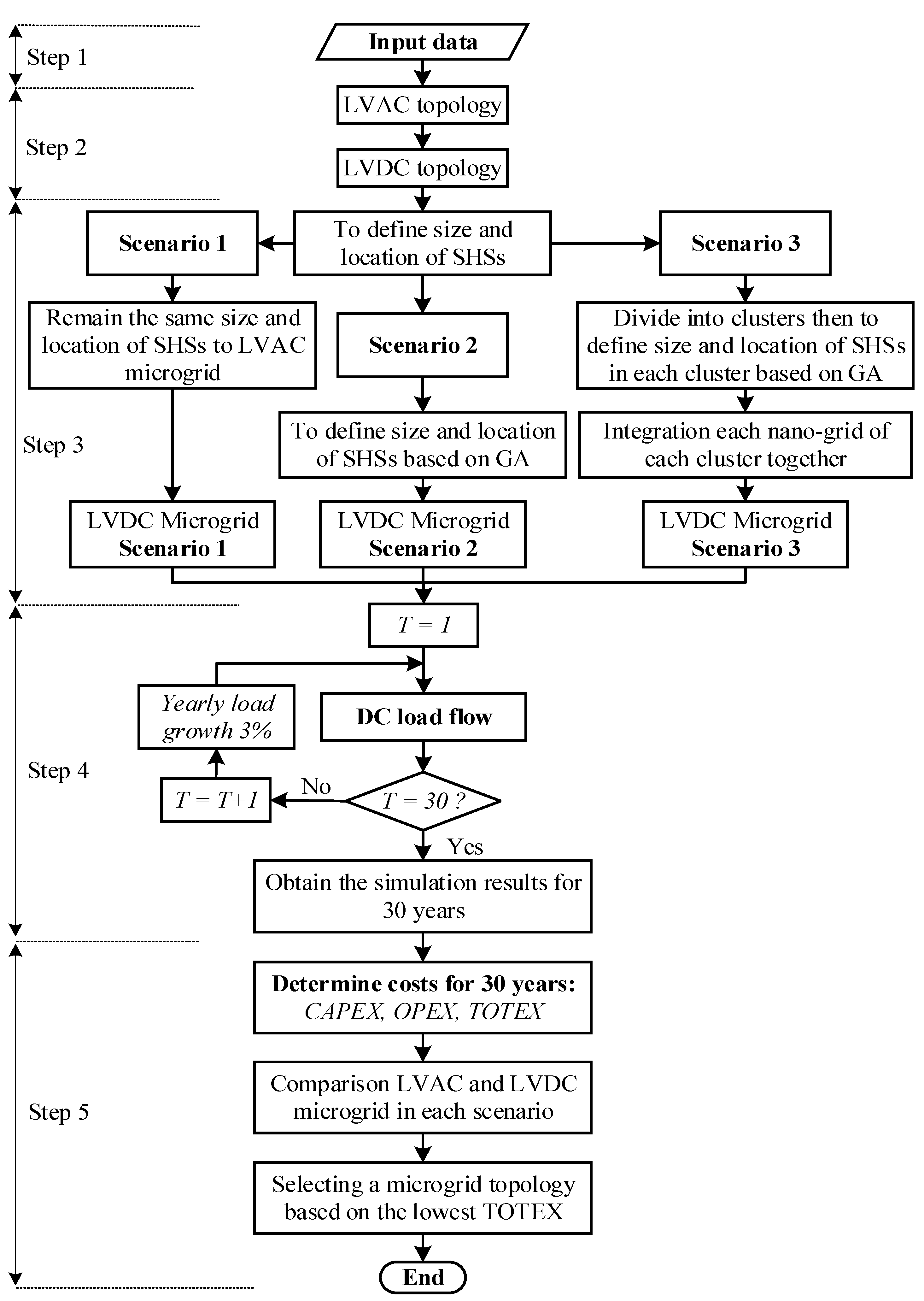
Figure 2.
An associated topology in XY coordinates containing the location of LV generator, electric poles, and all loads (households).
Figure 2.
An associated topology in XY coordinates containing the location of LV generator, electric poles, and all loads (households).
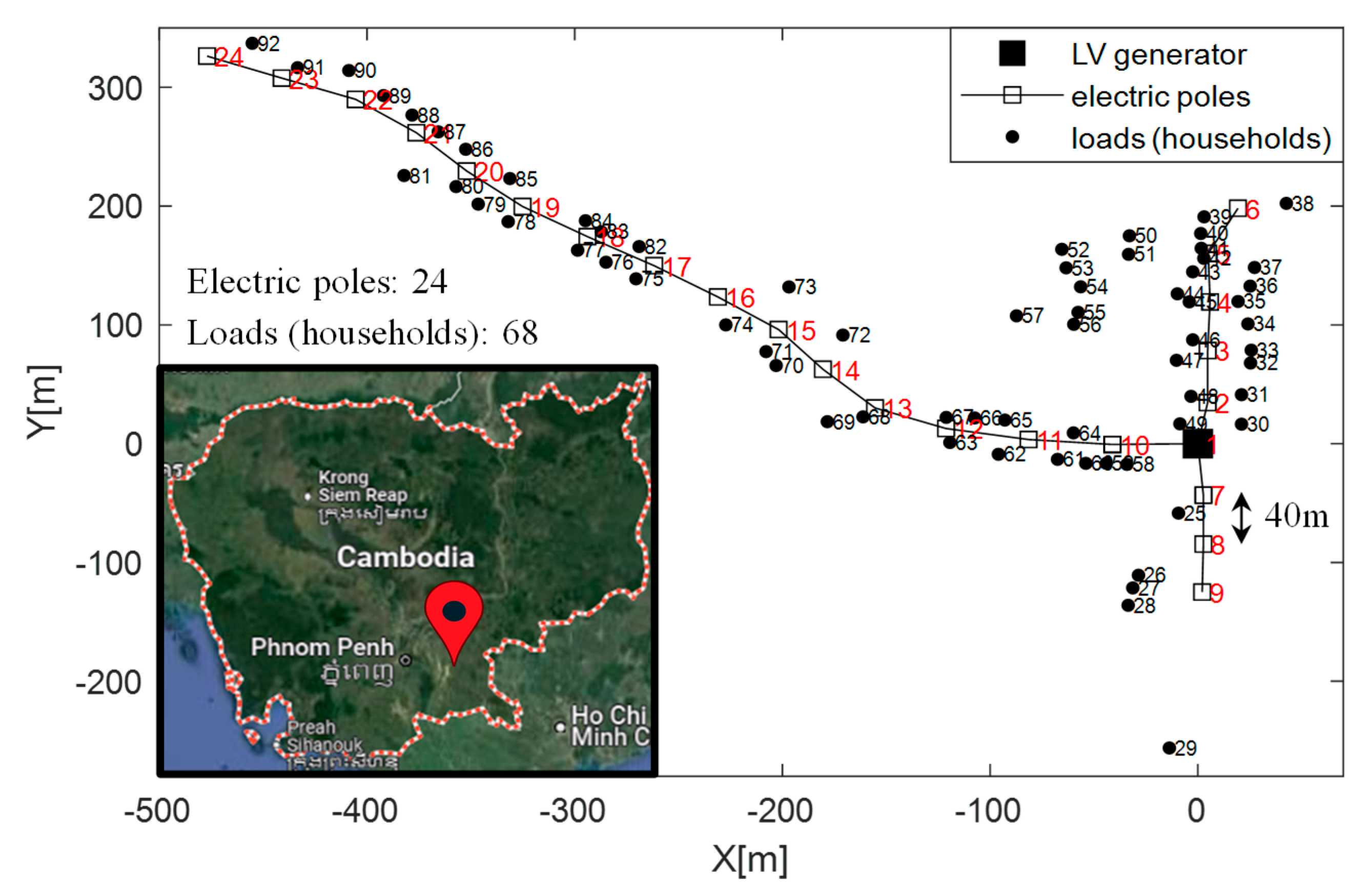
Figure 3.
The load, PV, and decentralized battery (DeBES) curve in pu.
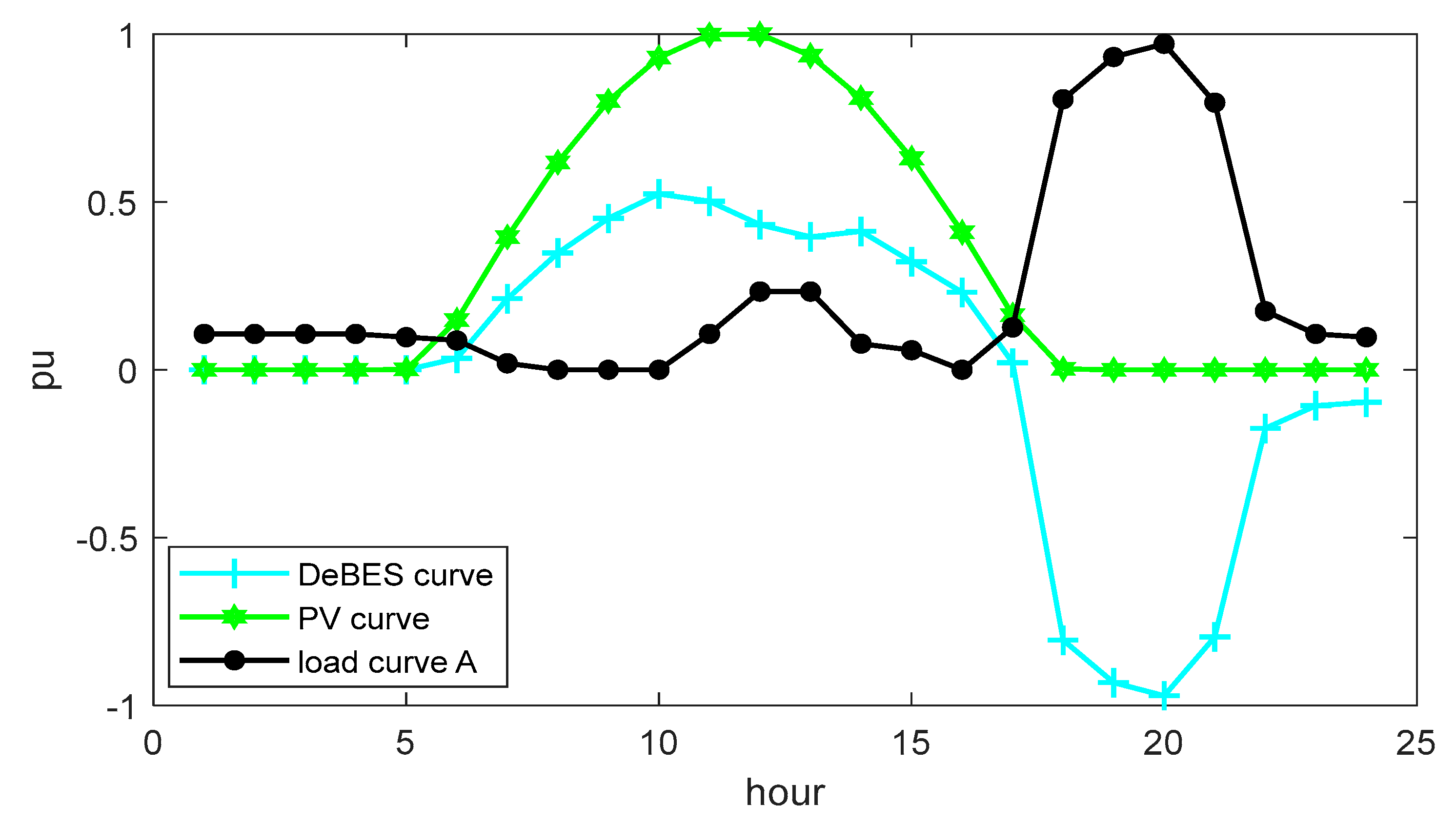
Figure 4.
LVAC radial topology.
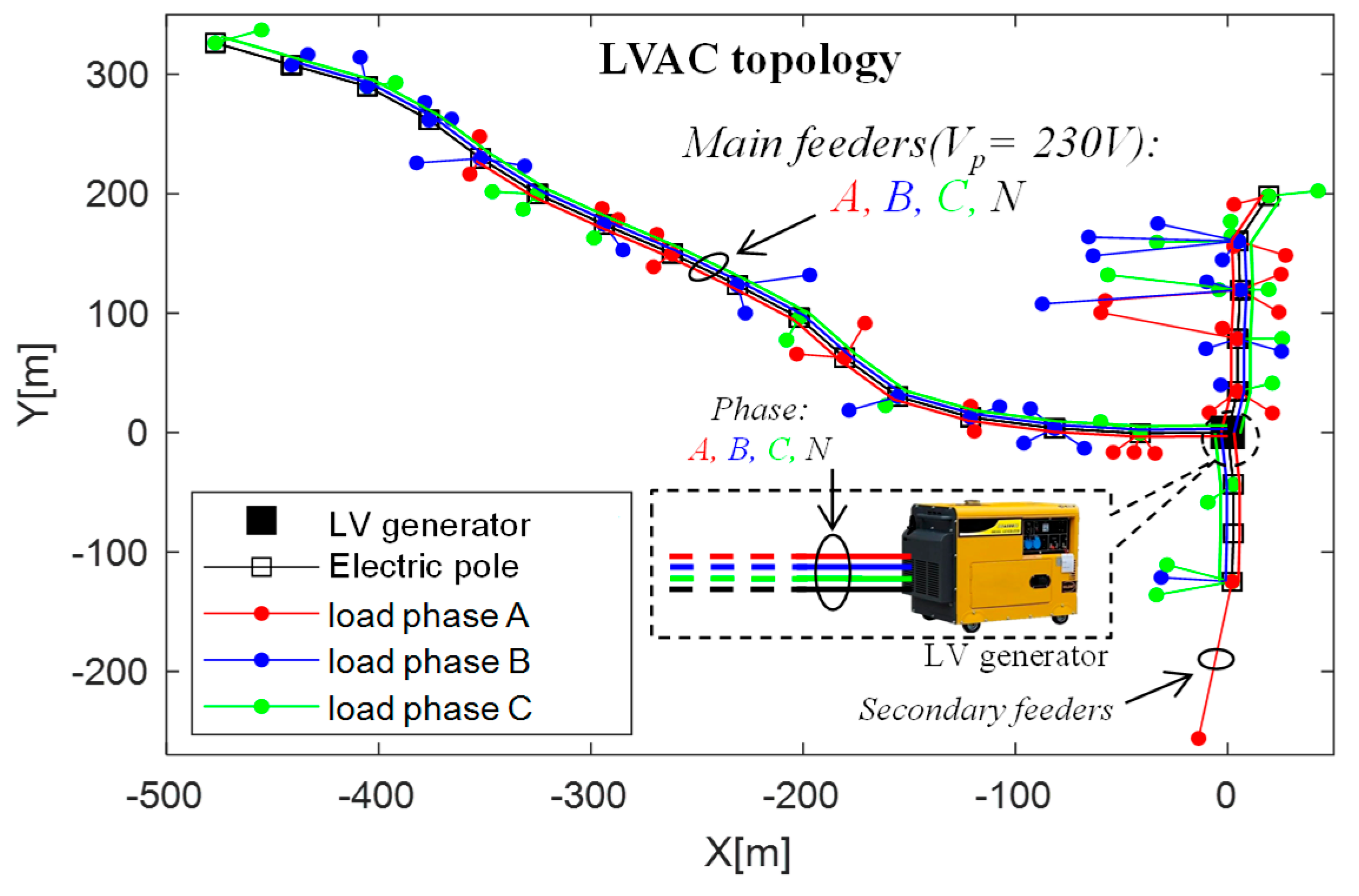
Figure 5.
Integrating SHSs with LVAC topology towards LVAC microgrid.
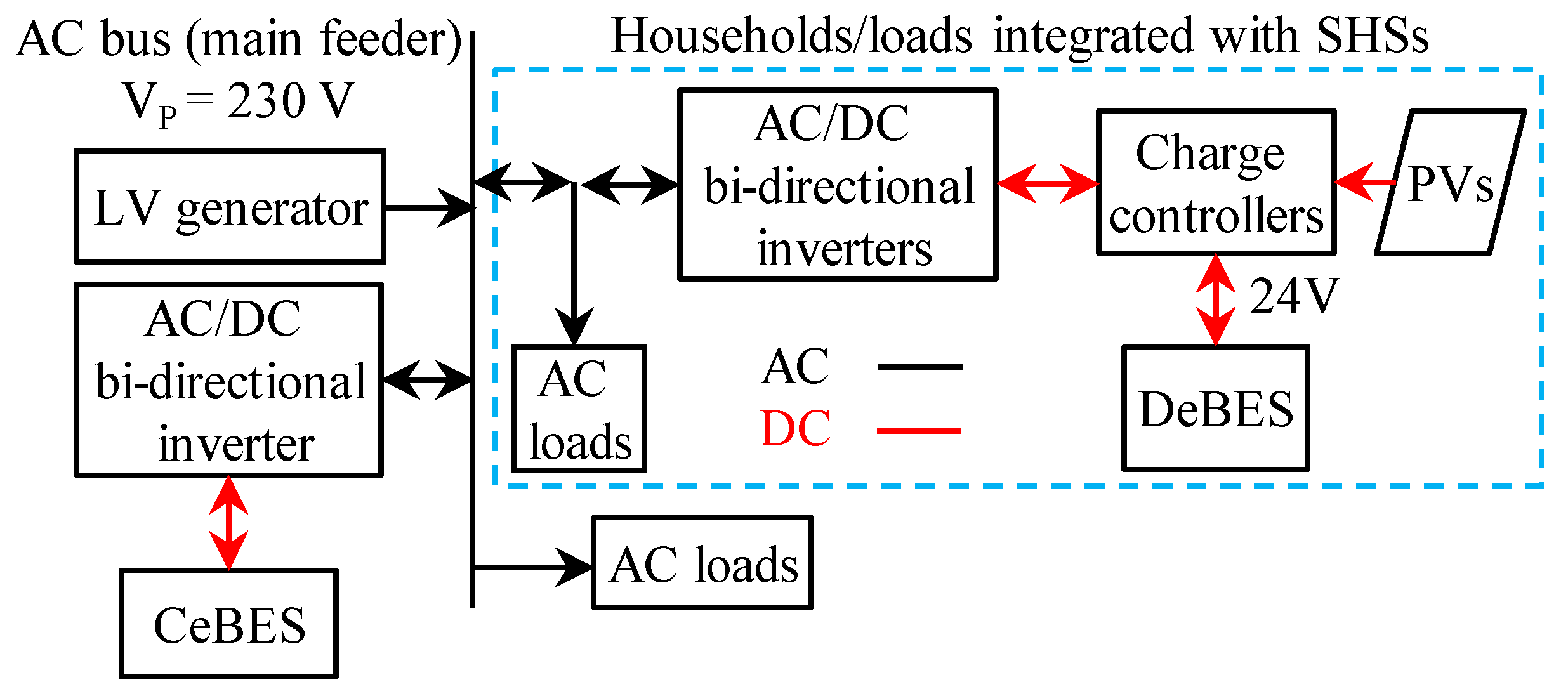
Figure 6.
LVDC topology based on LVAC structure for Scenario 1 and 2.
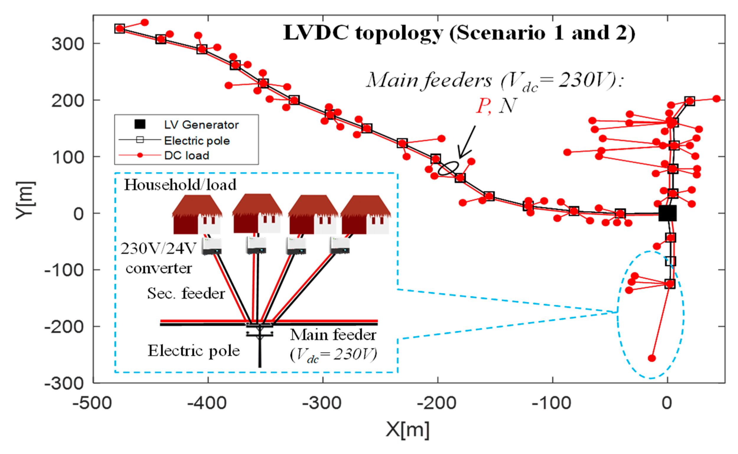
Figure 7.
The LVDC topology for Scenario 3.
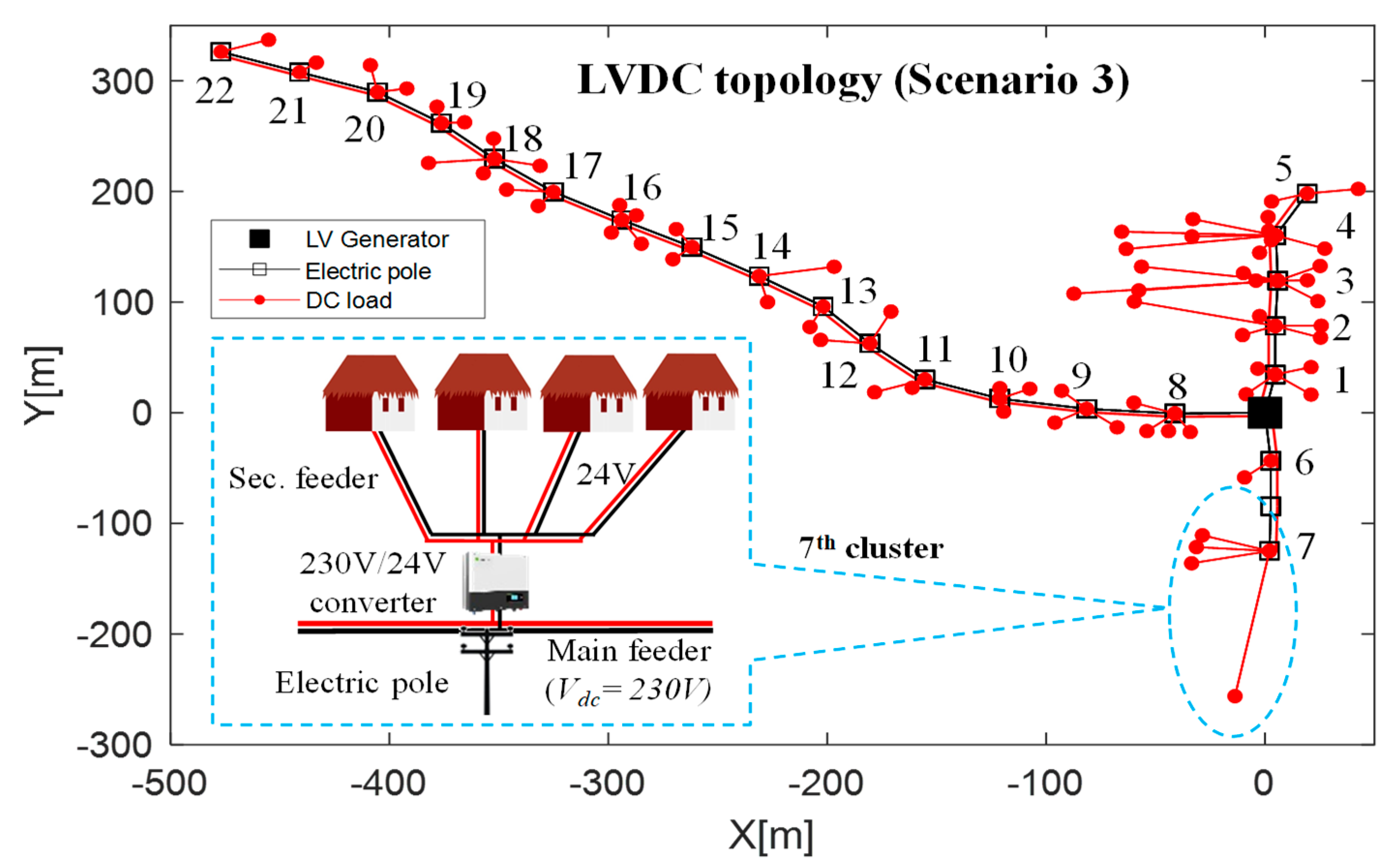
Figure 8.
The process of defining SHSs for each cluster.
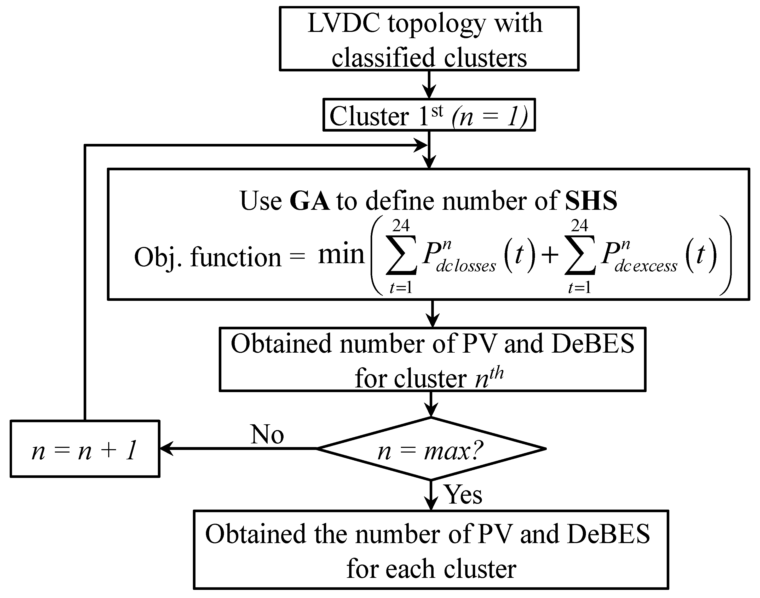
Figure 9.
The proposed diagram of integrating all nano-grids.
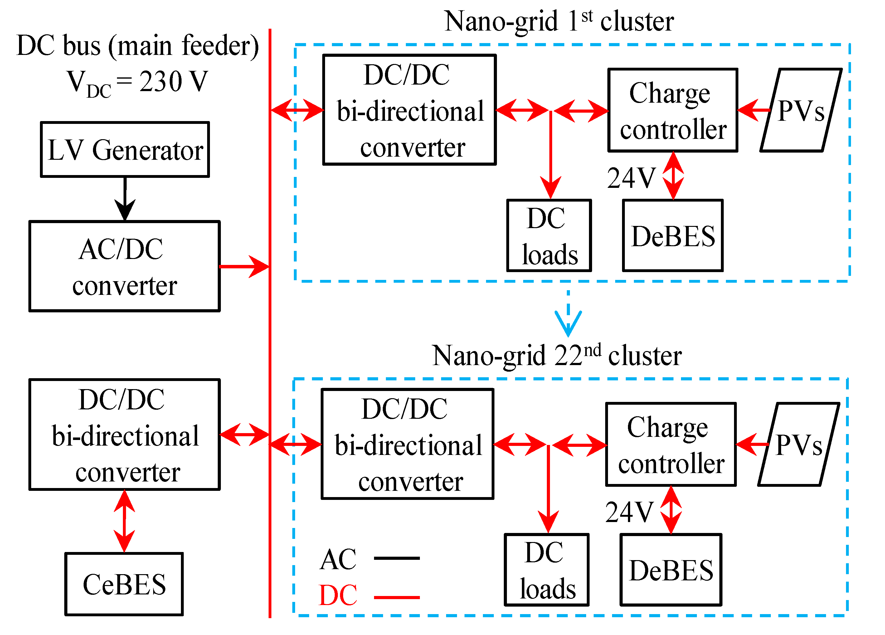
Figure 10.
The LVAC microgrid and LVDC microgrid in Scenarios 1, 2, and 3.
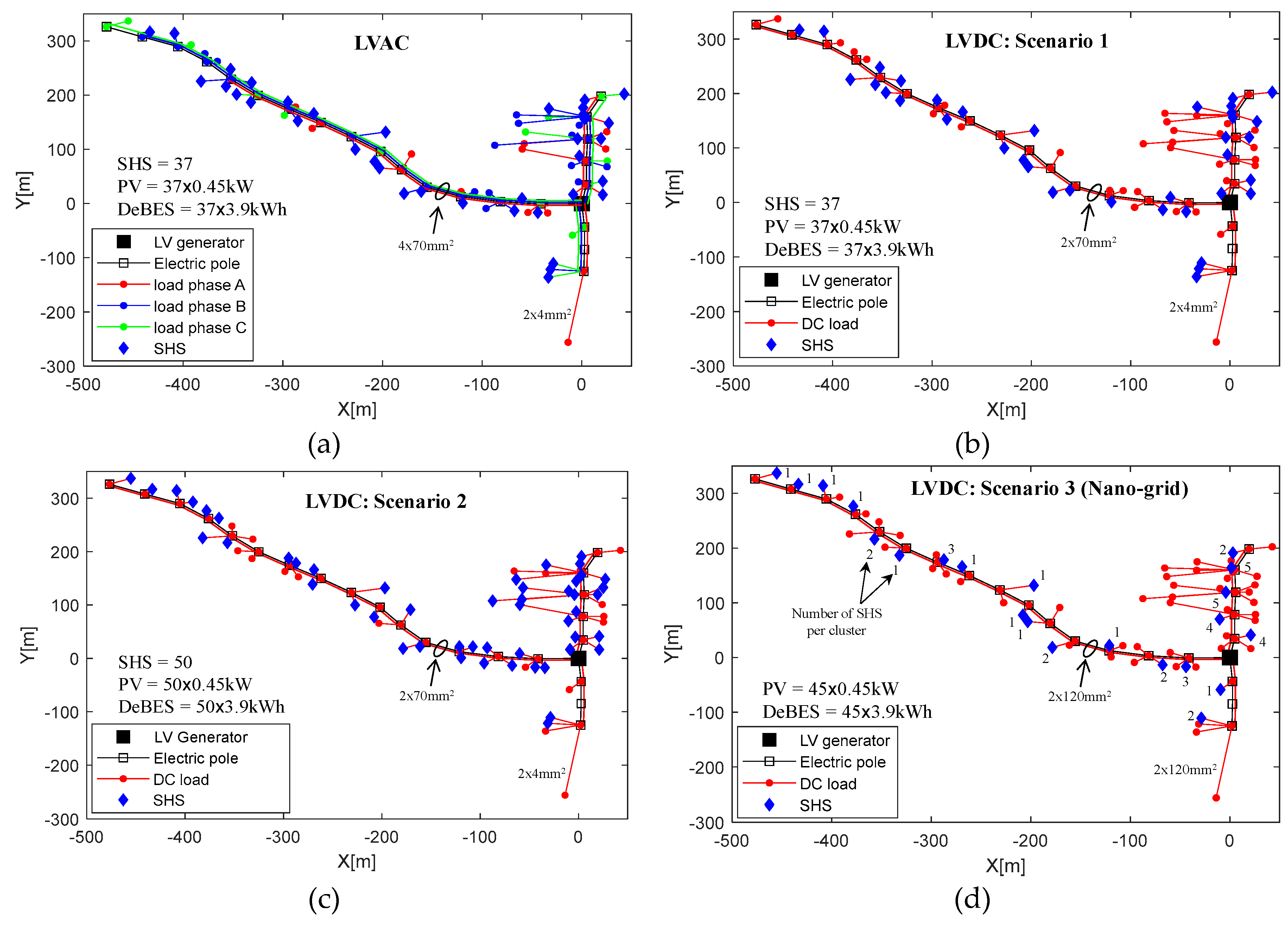
Figure 11.
Costs analysis for 30 years of each microgrid.
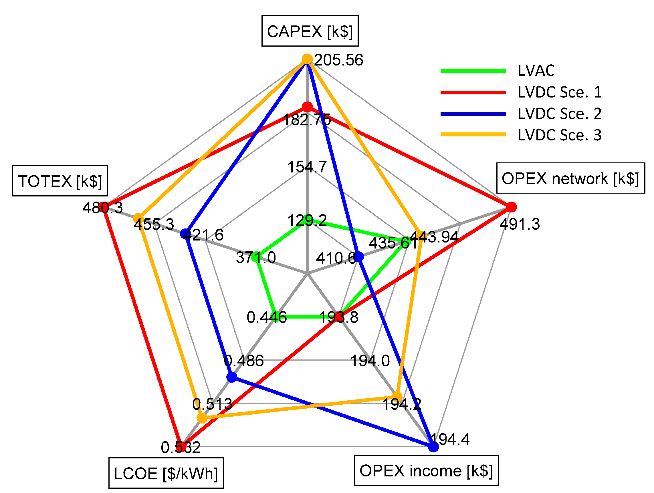
Figure 12.
Total investment costs and incomes for each microgrid for 30 years.
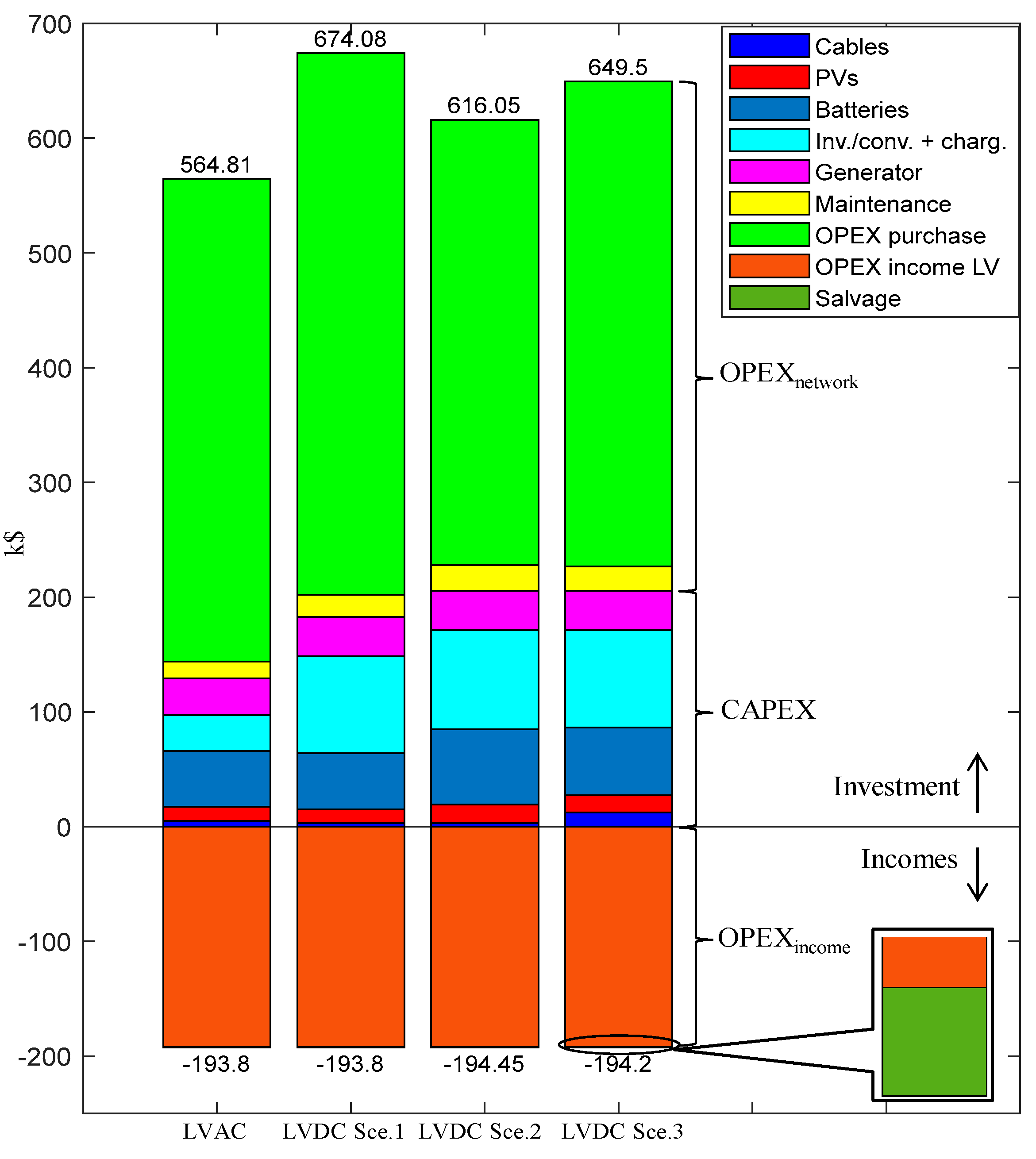

Table 1.
Input data for simulation.
| Items | Values | |
|---|---|---|
| Discount rate [40] | 6% | |
| Minimum and maximum voltage [44] | 0.9 pu or 1.1 pu | |
| Cost of fuel [8] | 0.495 $/kWh | |
| Cost of selling energy to households [45] | 0.152 $/kWh | |
| PV cost [8] | 600 $/kW | |
| DC charge controller [46] | 30 $/piece | |
| Battery cost [8] | 105 $/kWh | |
| Single-phase bi-directional inverter or converter [47] | 400 $/kW | |
| Three-phase bi-directional inverter or converter [48] | 820 $/kW | |
| DC cable length used per SHS | 10 m/SHS | |
| Maintenance cost (PV+battery+inverter/converter+charge controller) [49] | 11.5 $/kW/year | |
| LV generator cost [8] | 500 $/kW | |
| Efficiency of charge controller, inverter/converter, and battery [2,8,50] | 95% | |
| Degradation of charge controller, inverter/converter, PV, and battery [2] | 0.5% /year | |
| Lifespan of battery [2,8] | 5 years | |
| Lifespan of charge controller, inverter/converter, and LV generator [2,8] | 15 years | |
| Lifespan of PV panels [2] | 25 years | |
| Cable costs (1 core) [51] | 4 mm2 | 76 $/km |
| 70 mm2 | 1330 $/km | |
| 120 mm2 | 2280 $/km |
Table 2.
Input data for simulation.
| Items | LVAC | LVDC Sce.1 | LVDC Sce.2 | LVDC Sce.3 |
|---|---|---|---|---|
| Total number of SHS | 37 | 37 | 50 | 45 |
| Total PV output power (12:00) [kW] | 16.65 | 16.65 | 22.5 | 20.25 |
| Total max. DeBES power (20:00) [kW] | 23.9 | 23.9 | 32.3 | 29 |
| Total size of DeBES [kWh] | 144.3 | 144.3 | 195 | 175.5 |
Table 3.
Performance indicators.
| Items | LVAC | LVDC Scenario 1 |
LVDC Scenario 2 |
LVDC Scenario 3 |
|
|---|---|---|---|---|---|
| Vmin at 30th year [pu] | 0.97 | 0.90 | 0.91 | 0.91 | |
| EPV [MWh] | 1090.74 | 1090.74 | 1473.87 | 1326.4 | |
| Egenerator [MWh] | 2258.41 | 2536.28 | 2175.74 | 2330.6 | |
| Energy reversed at generator bus [MWh] | 0.145 | 0.134 | 0.23 | 0.22 | |
| Eloads [MWh] | 3120.5 | 3120.5 | 3120.5 | 3120.5 | |
| Losses [MWh] | SHSs | 202.49 | 472.53 | 504.9 | 493.73 |
| Main and sec. feeder | 26.27 | 34.14 | 24.37 | 37.14 | |
| Total | 228.76 | 506.67 | 529.27 | 530.87 | |
| CeBES [kWh] | 3.9 | 3.9 | 3.9 | 3.9 | |
| CO2 emissions [tone] | 2909.6 | 3262.5 | 2819.2 | 3003.6 | |
| Autonomous Ener. [%] | 32.5 | 30.0 | 40.3 | 36.2 | |
| Gradual electrification | No | No | No | Yes | |
Disclaimer/Publisher’s Note: The statements, opinions and data contained in all publications are solely those of the individual author(s) and contributor(s) and not of MDPI and/or the editor(s). MDPI and/or the editor(s) disclaim responsibility for any injury to people or property resulting from any ideas, methods, instructions or products referred to in the content. |
© 2026 by the authors. Licensee MDPI, Basel, Switzerland. This article is an open access article distributed under the terms and conditions of the Creative Commons Attribution (CC BY) license (http://creativecommons.org/licenses/by/4.0/).
Copyright: This open access article is published under a Creative Commons CC BY 4.0 license, which permit the free download, distribution, and reuse, provided that the author and preprint are cited in any reuse.


