Submitted:
04 February 2026
Posted:
05 February 2026
You are already at the latest version
Preprints on COVID-19 and SARS-CoV-2
Abstract
Background: Tooth loss is a relevant oral health indicator among older adults, as it captures cumulative disadvantage and has demonstrated patterning by race/ethnicity and socioeconomic conditions. How these geographic disparities evolved during the COVID-19 period has received less attention.
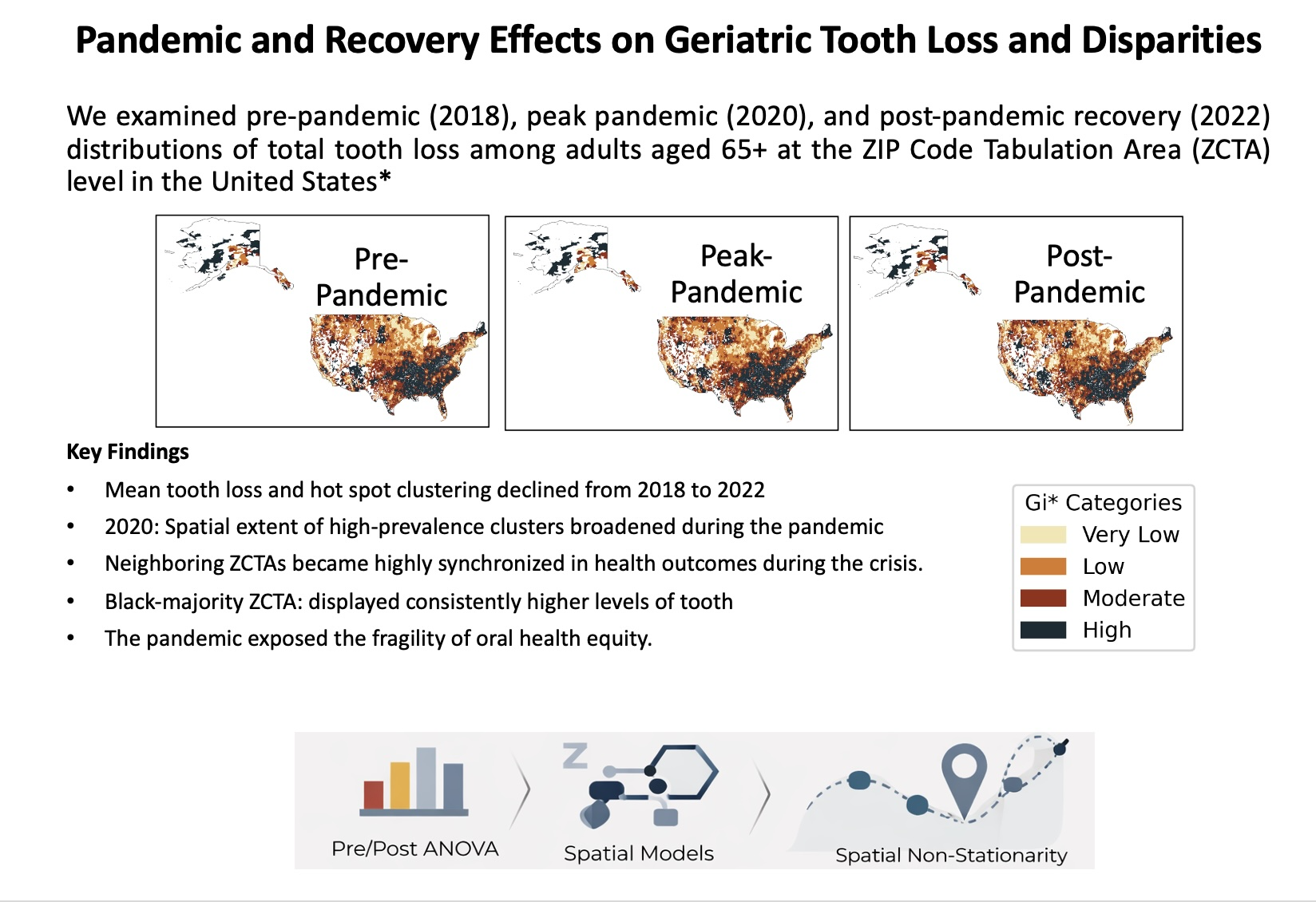
Objective: We aimed to describe changes in the spatial distribution of total tooth loss among adults aged ≥65 years in the United States across three time periods: pre-pandemic (2018), peak-pandemic (2020), and post-pandemic recovery (2022) at the ZIP Code Tab-ulation Area (ZCTA) level.
Methods: We conducted repeated cross-sectional ecological analyses, linking CDC PLACES estimates of tooth loss prevalence to ZCTA-level covariates from the American Community Survey for 2018, 2020, and 2022 (contiguous US). We summarized year-specific distributions, estimated pooled OLS models with year and year×race/ethnicity-majority interactions, and fitted year-specific spatial models (SLM/SEM), geographically weighted regression (GWR), and Getis–Ord Gi* hot spot analyses with Queen contiguity weights.
Results: Mean prevalence decreased from 15.9% (2018) to 14.4% (2022), and geographic clustering persisted across years. Black-majority ZCTAs consistently had higher preva-lence than other majority categories. Spatial dependence was strongest in 2020, when spatial lag effects were larger and GWR results suggested substantial geographic het-erogeneity in the associations between socioeconomic covariates and tooth loss. Hot spot maps reveal persistent clustering in the Southeast region, with a wider spatial footprint in 2020 and partial re-emergence of cold spots by 2022.
Conclusions: Tooth loss prevalence remained geographically clustered and unevenly distributed across the pre-pandemic, peak-pandemic, and recovery years examined. The pandemic period was associated with stronger spatial dependence and wider geographic clustering of high-prevalence areas, highlighting the importance of place-sensitive oral health strategies.
Keywords:
spatial epidemiology
; tooth loss
; geographically weighted regression
; hot spot analysis
; spatial lag model
; spatial error model
1. Introduction
Total tooth loss (edentulism) among older adults represents a major public health issue that greatly impacts overall health, quality of life, and longevity [1,2]. It is a condition that disproportionately affects vulnerable populations, reflecting broader societal inequities [3,4]. Complete tooth loss in individuals leads to a decline in nutritional intake because people tend to eat softer foods which lack nutritional value and may result in malnutrition as well as other health issues [1,2.5]. Tooth loss leads to cognitive impairments such as dementia and Alzheimer's disease [6,7] and results in social isolation which affects mental health [8,9]. Recent studies show tooth loss functions as an indicator of shorter life expectancy which emphasizes the vital connection between oral health and overall systemic health [10,11,12].
The existing evidence highlights socioeconomic and racial differences in tooth loss frequency among older populations [3,4,13]. The socioeconomic status of individuals plays a defining role since those from low-income backgrounds encounter major obstacles to dental care access which results in untreated dental issues and increased edentulism risk [3,4,14]. Non-Hispanic Black and Hispanic populations experience higher tooth loss rates than other groups when education and income levels are accounted for [13,15,16]. The disparity in dental care access is intensified by various contextual elements including geographic location and the socioeconomic conditions within communities which affect dental service access and health education [3,14].
The reduction of tooth loss rates in developed nations stems from better dental treatments and preventive practices yet these benefits have not reached all communities equally [17]. Disparities based on socioeconomic status and race persist, and in some cases, may be widening [15,18,19]. While these disparities are often reported as national averages, they are fundamentally rooted in the physical environment where individuals live and age. To understand how these disparities evolve over time we must adopt a longitudinal perspective which enables the study of temporal changes and identification of factors behind ongoing or growing inequities.
Traditional analyses of tooth loss that ignore spatial relationships fail to properly address the complex connections between individual-level risk factors and geographic locations of individuals [20]. Analyzing spatial patterns of tooth loss through geospatial methods helps identify geographic clusters while understanding how location influences oral health results and overcoming traditional aspatial analytical limitations [21,22]. Geographic Information Systems (GIS) uncover localized tooth loss patterns which remain hidden in broader aggregate data and pinpoint areas with high prevalence caused by dental care access issues and transportation barriers along with community resource challenges [21,22,23]. An accurate region-based understanding enables effective design of specific interventions while ensuring resources are distributed properly. However, identifying where clusters exist is only the first step; understanding why they persist or expand requires moving beyond static, single-point observations.
Cross-sectional studies provide valuable information about prevalence at specific points but lack capability to determine causation or examine how socioeconomic/racial factors interact with tooth loss over time [24].Cross-sectional studies cannot establish if low SES leads to tooth loss or whether tooth loss results in low SES and fail to measure how life-course factors cumulatively affect oral health [25,26]. In contrast to cross-sectional studies, longitudinal analysis enables researchers to track temporal changes in these relationships and assess how disparities develop over time and the effectiveness of interventions [15,27].
The timeframe from 2018 to 2022 presents a crucial window to study variations in tooth loss disparities. This timeframe encompasses the COVID-19 pandemic, which profoundly disrupted healthcare access and utilization, potentially exacerbating existing inequities in dental care, especially for vulnerable populations [28,29]. During this timeframe socioeconomic conditions and public health priorities changed while the correlation between these changes and oral health outcomes became essential to evaluate [30]. Given this volatility, there is an urgent need for research that maps these changes with high geographic precision.
1.1. Study Objectives and Novelty
Building on this need, the present research addresses important literature voids through a comprehensive longitudinal geospatial investigation of total tooth loss in the U.S. geriatric demographic at ZIP Code Tabulation Areas (ZCTAs) from 2018 through 2022. The research evaluates how the geographic distribution of total tooth loss in older adults changed during the years studied while mapping it across these periods. The research examines the evolution of socioeconomic and racial factors' correlation with total tooth loss while determining if specific regions show growing or shrinking tooth loss disparities over time. The research examines how specific socioeconomic risk factors have evolved in their importance for geographic tooth loss variation from 2018 to 2022, with a focus on identifying the characteristics of regions where these patterns are most pronounced. Our aim is to describe how spatial patterning and associations with race/ethnicity and socioeconomic context shifted across the pre-pandemic (2018), peak-pandemic (2020), and recovery (2022) periods, rather than to estimate a causal effect of the pandemic.
Our research provides multiple contributions to the existing body of oral health disparities literature. First, we integrate CDC PLACES and ACS data at the ZCTA level and for three time points (2018, 2020, 2022) in order to capture a more fine-grained view of how geographic patterning and correlates of geriatric tooth loss may have shifted across pre-pandemic, peak-pandemic, and recovery periods. Second, we employ a complementary set of spatial approaches (Moran’s I and Getis–Ord Gi* for clustering, spatial lag and spatial error models for dependence, and geographically weighted regression (GWR) to characterize spatial non-stationarity) in order to move beyond the national average and identify where associations may differ across place. Third, by examining tooth loss in relation to racial/ethnic composition and socioeconomic context during a period of major disruption, we help identify where inequities appear to persist or expand, and we situate tooth loss as part of a broader profile of later-life health risk, including multimorbidity. [31,32,33,34]
Taken together, these results begin to clarify how place, social conditions, and racialized patterns of disadvantage may intersect with tooth loss among older adults. This kind of geographic specificity can be valuable for directing prevention and access efforts (especially where clustering remains) rather than assuming a homogeneous national pattern.
2. Materials and Methods
2.1. Overview of Data Sources and Study Area
We used ZCTA-level demographic, socioeconomic, and health indicators to examine geriatric total tooth loss across three periods: pre-pandemic (2018), peak pandemic (2020), and post-pandemic recovery (2022). Covariates representing socioeconomic and demographic measures were obtained from 5-year estimates of the American Community Survey (ACS) for 2018, 2020, and 2022. The outcome of total tooth loss prevalence among adults (≥65 years) was obtained from CDC PLACES for the respective years. ZCTA boundary files were obtained from TIGER/Line shapefiles for 2018, 2020, and 2022 to construct spatial weights.
2.2. Data Integration and Preparation
The PLACES data were merged to the ACS ZCTA file using the ZCTA identifier for each year (2018 PLACES + 2018 ACS; 2020 PLACES + 2020 ACS; 2022 PLACES + 2022 ACS). The resulting analytic samples contain 30,358 ZCTAs in 2018, 29,808 in 2020, and 29,760 in 2022, and represent ZCTAs with non-missing PLACES tooth loss and ACS covariates after merging.
We performed complete-case analysis, dropping observations with missing values on variables used in our models. The number of dropped observations was small. Continuous predictors were standardized (mean 0, SD 1). For pooled OLS, means/SDs were computed on the stacked dataset. We defined a race/ethnicity “majority category” using a plurality rule (largest share among White, Black, Hispanic, and Other) and modeled it using indicator variables, with a Hispanic majority as the reference category.
2.3. Statistical and Spatial Analyses
Analytic strategy: We used a step-wise analytic approach to address a series of related questions. Pooled OLS models were used to provide a global baseline and to summarize the average associations across years. Global Moran's I was used to assess for spatial dependence and Getis–Ord Gi* for visual interpretation. To quantitatively assess the presence of spatial dependence in a regression framework we fit year-specific spatial lag (SLM) and spatial error (SEM) models. GWR was used as the primary approach to assess for spatial non-stationarity in covariate associations and to summarize geographic variation in local coefficients.
Descriptive statistics (mean, median, standard deviation, and percentiles) were calculated separately for each year. Mean differences in tooth loss prevalence across 2018, 2020, and 2022 were assessed using one-way ANOVA with post hoc Tukey HSD comparisons.
We applied pooled OLS models to stacked ZCTA–year observations (n = 89,926) in order to assess the association between the covariates and tooth loss prevalence. Models included indicators for year, and in the interaction specification, year–race/ethnicity majority terms (2018 and Hispanic-majority ZCTAs were the reference categories). Variance inflation factors and the condition number were used to assess multicollinearity. All hypothesis tests were two-sided with α = 0.05.
Spatial weights were defined using Queen contiguity on year-specific ZCTA polygons (TIGER/Line 2018, 2020, 2022) which allowed ZCTAs to become neighbors when they possessed a shared boundary or vertex. The resulting contiguity-based weights matrix was used for Global Moran’s I, Getis–Ord Gi*, as well as year-specific spatial lag (SLM) and spatial error (SEM) models. The contiguity weights matrix W was row-standardized (row sums = 1), so Wy represents the average of neighboring ZCTA values.
Spatial autocorrelation in tooth loss prevalence was measured using Global Moran’s I for each study year. Spatial regression models were estimated separately for each year to account for changes in spatial patterns of dependence over time. Models were estimated using spatial lag (SLM) and spatial error (SEM) specifications. For the SLM, we modeled spatial dependence in the outcome as , where is the dependent variable (tooth loss percentage), ρ is the spatial lag coefficient, Wy represents the spatially lagged dependent variable, is a matrix of independent variables, β is a vector of regression coefficients, and ε is the error term. Direct, indirect, and total effects were calculated for each predictor variable. For SEM we used with, where captures spatial dependence in the error process. We used SLM/SEM results to interpret whether the spatial patterns observed in Geographically weighted regression (GWR) coincided with outcome spillovers (SLM) or spatially structured unobservables (SEM), rather than treating these models as competing alternatives.
GWR models were fit for each year to characterize spatially varying associations between covariates and tooth loss prevalence. The GWR model can be expressed as: where are the coordinates of the ith ZCTA, is the intercept, are the local regression coefficients for the kth predictor variable at location is the value of the predictor variable at location , and is the error term. A Gaussian kernel function and AICc-based bandwidth selection were used. Coordinates were derived from PLACES geolocation points (longitude/latitude; EPSG:4326).
Spatial analyses were implemented in Python using GeoPandas and PySAL.
3. Results
3.1. Descriptive Statistics: Tooth Loss Prevalence
Across U.S. ZIP Code Tabulation Areas (ZCTAs), total tooth loss prevalence among adults aged 65 and older declined over time. The mean prevalence decreased from 15.9% (2018) to 15.3% (2020) and then to 14.4% (2022), and the median declined from 15.0% (2018) to 14.5% (2020) and then to 13.4% (2022). Dispersion was comparable across years (standard deviation (SD): 6.1 in 2018, 5.6 in 2020, 6.4 in 2022), though in 2020 there reduction in dispersion. The interquartile range also declined during the observed period, the 25th percentile decreased from 11.7% (2018) to 11.4% (2020) and then to 9.9% (2022), and while the 75th percentile decreased from 19.2% (2018) to 18.4% (2020) and then to 17.7% (2022). Observed minima were 3.0% (2018), 3.3% (2020), and 1.9% (2022) while maxima were 59.9% (2018), 53.9% (2020), and 56.8% (2022).
Figure 1 (kernel density estimates) shows that the distribution's peak moved to the left side from 2018 to 2022, which is in line with the overall decrease in prevalence of dental loss. The total tooth loss prevalence distribution exhibited less dispersion in 2020 when compared to the distributions from 2018 and 2022.
3.2. Descriptive Statistics: Covariates
Covariates exhibited time-varying trends which is consistent with broad socioeconomic changes. The educational attainment rate has increased during the period studied: the average percentage of adults over 65 years of age who completed secondary education has increased from 61.4% (2018) to 62.8% (2022), and the average number of bachelor's degree or higher has increased from 21.2% to 23.7%. The median household income has risen from $59,187 (2018) to $73,352 (2022), in line with rising monthly costs for housing (from $925 to $1,088). The average proportion of residents over the age of 65 increased from 18.6% to 20.2%, while the average number of over 65s per unit remained stable at 0.5%. The average uninsured rate for adults aged over 65 remained low and stable (0.6%). The average poverty rate of adults aged over 65 years has increased slightly (9.4% to 10.0%). The female population proportion decreased slightly (53.7% to 53.2%). Table A2 presents year-wise mean, median, and variability measures for key socioeconomic and demographic indicators at the ZCTA level to contextualize temporal structural changes.
3.3. ANOVA and Pairwise Comparisons
A one-way ANOVA revealed that there were statistically significant differences in the means of tooth loss prevalence between years (F= 417.64, p < 0.001). Tukey HSD post-hoc tests showed that all pairwise comparisons were statistically significant (p < 0.001): 2018 vs 2020 (mean difference −0.6, 95% CI [−0.7, −0.5]), 2018 vs 2022 (mean difference −1.4, 95% CI [−1.5, −1.3]), and 2020 vs 2022 (mean difference −0.8, 95% CI [−0.9, −0.7]). Table A3 provides Tukey HSD post hoc comparisons of total tooth loss across study years, detailing pairwise differences and confidence intervals not shown in the main results.
3.4. Ordinary Least Squares (OLS) Regression: Without Interaction Terms
In pooled OLS models without interaction terms (n = 89,380 ZCTA-year observations), covariates explained a substantial proportion of variation in tooth loss prevalence (R² = 0.609; adjusted R² = 0.609; F = 9,943; p < 0.001; AIC = 492,437; BIC = 492,578; Table 1). Unless stated otherwise, p-values are two-sided.
Clear directional patterns emerged (Table 1). Variables associated with higher tooth loss included: percent uninsured among adults ≥65 (β = 0.0419, 95% CI [0.03, 0.054], p < 0.001), adults ≥65 per housing unit (β = 5.5219, 95% CI [5.207, 5.837], p < 0.001), percent below poverty among adults ≥65 (β = 0.0723, 95% CI [0.069, 0.076], p < 0.001), and race/ethnicity-majority indicators relative to the omitted reference category (White-majority: β = 2.88, Black-majority: β = 7.48, Other-majority: β = 7.30; all p < 0.001). Variables associated with lower tooth loss included educational attainment (high school: β = −0.112, bachelor’s or higher: β = −0.131; both p < 0.001), higher percentage of residents aged ≥65 (β = −0.1485, p < 0.001), higher monthly housing costs (β = −0.003, p < 0.001), and higher median income (β = -6.56E-05, 95% CI [-6.74E-05, -6.38E-05], p < 0.001). Female percentage among adults ≥65 was not associated with tooth loss in this model (β = 0.0014, p = 0.733).
Year indicators (relative to 2018) were statistically significant (2020: β = 0.0933, 95% CI [0.032, 0.155], p = 0.003; 2022: β = 0.4515, 95% CI [0.388, 0.515], p < 0.001), reflecting conditional differences after covariate adjustment.
3.5. OLS Regression with Year × Race/Ethnicity-Majority Interactions
The interaction model (n = 89,380) remained strongly significant (R² = 0.596; adjusted R² = 0.596; F = 7,769; p < 0.001; AIC = 495,268; BIC = 495,437; Table 2). Main-effect directions for socioeconomic variables were consistent with the non-interaction model: uninsured percentage (β = 0.042, p < 0.001) and poverty (β = 0.0772, p < 0.001) were positively associated with tooth loss, whereas education (high school β = −0.113, bachelor’s or higher β = −0.1314) and income (β = −6.73E-05) were negatively associated (all p < 0.001).
Year indicators became negative in the presence of interactions (2020 vs 2018: β = −3.0848, 95% CI [−3.371, −2.799], p < 0.001; 2022 vs 2018: β = −2.2575, 95% CI [−2.535, −1.98], p < 0.001), indicating that year differences depend on the race/ethnicity-majority category.
Interaction terms showed large, positive differentials relative to the omitted race/ethnicity-majority reference group (Table 2). For 2020, interaction coefficients were: White-majority (β = 3.06, 95% CI [2.773, 3.349], p < 0.001), Black-majority (β = 7.108, 95% CI [6.75, 7.467], p < 0.001), and Other-majority (β = 6.095, 95% CI [5.671, 6.519], p < 0.001). For 2022, interactions were similarly positive: White-majority (β = 2.513, 95% CI [2.233, 2.793], p < 0.001), Black-majority (β = 7.5347, 95% CI [7.182, 7.887], p < 0.001), and Other-majority (β = 7.449, 95% CI [7.032, 7.867], p < 0.001). Female percentage in this model was statistically significant but small in magnitude (β = 3.30E-03, 95% CI [1.0E-03, 6.0E-03], p = 0.02).
3.6. Spatial Autocorrelation (Global Moran’s I)
Global Moran’s I shows strong spatial clustering of tooth loss prevalence during all years (Table 3). Clustering was strongest in 2018 and 2020 and remained substantial in 2022 (z-scores approximately 205.27, 212.74, and 184.59, respectively; all p < 0.001), consistent with non-random geographic patterning of high and low prevalence ZCTAs.
3.7. Hot Spot Analysis (Getis-Ord Gi)*
Hot spot analysis using the Getis–Ord Gi* statistic revealed statistically significant spatial clustering of high- and low-prevalence ZCTAs in 2018, 2020, and 2022 (Figure 2, Figure 3 and Figure 4). In pre-pandemic (2018), ZCTAs in the Southeast, Appalachia, and parts of the Midwest formed high-prevalence clusters, while those in the Northeast, the West Coast, and parts of the Upper Midwest formed low-prevalence clusters. In peak-pandemic (2020), the spatial distribution of high-prevalence clustering became more extensive geographically, with additional high-prevalence clusters observed in parts of the Midwest and South, while low-prevalence clusters were still observed but with less overall coverage. In post-pandemic (2022), ZCTAs with low prevalence formed clusters in parts of selected regions, while high-prevalence clustering was maintained in the Southeast and some rural areas. The maps of hot spot analysis outputs show evidence of spatial clustering in all three periods, with shifting geographic distributions of hot and cold spots over time (Figure 2, Figure 3 and Figure 4).
3.8. Spatial Lag Model (SLM)
Spatial lag models (SLM) exhibited statistically significant spatial dependence for all three time periods (Table 4, Table 5 and Table 6), which corresponded to the periods before, during, and after the pandemic (2018, 2020, and 2022, respectively). The size of the spatial dependence was not consistent, however.
Spatial dependence was statistically significant, yet relatively small, in the year before the pandemic (2018). Model fit was good (Pseudo R² = 0.719; AIC = 150,789), and the spatial lag parameter was small (ρ = 0.0617, SE = 0.0007, z = 89.05, p < 0.001; Table 4). The pre-pandemic pattern of statistical significance with small magnitude indicates that the spatial dependence was weakly present in the period before the pandemic, though most of the variation could have been attributable to variation between ZCTAs with the same characteristics.
Spatial dependence was substantially greater during the peak of the pandemic. The spatial lag coefficient was much larger, at ρ = 0.6452 (SE = 0.0043, z = 150.33, p < 0.001), and the model fit was slightly better (Pseudo R² = 0.7873; AIC = 143,483; Table 5). This increase in spatial dependence, both in terms of statistical significance and magnitude, is consistent with the idea that tooth loss prevalence was highly aligned with prevalence in surrounding ZCTAs during the pandemic, that is, ZCTAs with similar levels of tooth loss were more clustered than before or after the pandemic.
Spatial dependence was still statistically significant, and substantial, during the post-pandemic recovery period (2022). However, it was attenuated compared to 2020 (ρ = 0.5711, SE = 0.0052, z = 110.27, p < 0.001), and the model fit was worse (Pseudo R² = 0.7071; AIC = 153,664; Table 6). The spatial effects were smaller during the post-pandemic recovery period, but the magnitude did not return to what was observed in the year before the pandemic.
Direct/indirect decomposition revealed that multiple predictors had both within-ZCTA and spillover associations (Table 4). For example, in 2018, the total effect of adults ≥65 per housing unit was 5.7366 (direct 5.3827, indirect 0.3539), while total effects of the education measures were negative (high school total −0.0886; bachelor’s or higher total −0.1036). At the peak of the pandemic in 2020, indirect (spillover) components were substantially larger than in 2018 for multiple predictors (e.g., uninsured total 0.3208, with indirect 0.2070). This shift aligns with the elevated spatial lag parameter observed in 2020, indicating stronger cross-area linkage during this period. In 2022, effect directions were similar, although indirect components were generally smaller than in 2020, consistent with partial attenuation of spatial spillovers.
3.9. Spatial Error Model (SEM)
Spatial error models (SEM) revealed statistically significant residual spatial autocorrelation in all years of study (Table 7, Table 8 and Table 9), indicating continued evidence of spatial structure after accounting for observed covariates.
In 2018, before the start of the pandemic, λ = 0.7953 (SE = 0.0044, z = 178.99, p < 0.001), AIC = 142,360 and Pseudo R² = 0.6095 (Table 7). During the peak of the pandemic (2020), λ was similarly high (λ = 0.7881, SE = 0.0045, z = 175.57, p < 0.001; AIC = 144,176; Pseudo R² = 0.5867; Table 8). During the first full post-pandemic recovery year (2022), λ was lower, but still large (λ = 0.6830, SE = 0.0058, z = 118.41, p < 0.001; AIC = 154,568; Pseudo R² = 0.5457; Table 9).
SEM results overall indicate continued evidence of spatial structure in the data after accounting for measured covariates throughout the study period, especially before and during the peak pandemic year. These results should be interpreted with caution, as changes in λ may also reflect broader changes in the regional environment not specific to any single area’s relationships.
3.10. Geographically Weighted Regression (GWR)
Given the evidence of spatial dependence and clustering, we next examined whether covariate associations varied across space using GWR. GWR models had improved fit compared to the corresponding global regressions during all three time periods (Table 10, Table 11 and Table 12), consistent with spatially varying associations. GWR in the year before the pandemic began (2018) had R² = 0.898 and adjusted R² = 0.872 compared with the global regression R² = 0.618 (Table 10). Fit remained high during the peak year of the pandemic (2020) (R² = 0.877; adjusted R² = 0.847; Table 11). Fit during the post-pandemic recovery year (2022) declined but remained high (R² = 0.816; adjusted R² = 0.781; Table 12).
Local coefficient summaries reinforce this picture (Table 10, Table 11 and Table 12). The distributions of local estimates (mean, SD, and min/median/max) showed wide geographic spread in effect size, and for some predictors, coefficients appear to change sign across regions. In practical terms, a predictor that looks “protective” in one part of the country may be weak, null, or even reversed elsewhere. That kind of variability is consistent with place-specific contexts, although it could also reflect sensitivity to local sample density or bandwidth choices rather than purely substantive differences.
Overall, across pre-pandemic, peak pandemic, and recovery periods, GWR results indicate persistent geographic variation in predictor–outcome relationships that global models are likely to average away (Table 10, Table 11 and Table 12).
Additional spatial diagnostics and model comparisons are provided in the Appendix. The Table A4 compares the relative performance of Spatial Lag and Spatial Error models across years using standard model fit criteria, and Table A5 reports year-specific estimates of spatial dependence parameters (rho and lambda), which highlights shifts in the dominant sources of spatial autocorrelation over time. Table A6 summarizes variations in key socioeconomic predictors across spatial models and study years, with spillover effects most pronounced in 2020 and attenuating by 2022.
4. Discussion
This study examined ZCTA-level disparities in geriatric tooth loss across three periods: pre-pandemic (2018), peak pandemic (2020), and post-pandemic recovery (2022). In this study we assessed how socioeconomic factors, racial composition, and spatial dependence were associated with tooth loss prevalence over time. For this purpose, we purposefully combined global and local modeling approaches. Pooled OLS models provide an estimate of the average association and allow for comparability across years, while SLM/SEM models correct for spatial dependence, which can bias standard regression results. GWR then adds to these results by identifying where associations are stronger, weaker, or even inverted, which has the potential to inform place-specific vulnerability and recovery trajectories.
4.1. Overall Trends and Persistent Disparities
Although the mean and median tooth loss percentages decreased over the study period, possibly reflecting improvements in dental care access or preventative measures (more research is needed to confirm these particular drivers), the rising standard deviation in post-pandemic (2022) combined with the continuous right tail in the KDE graphs indicates a widening of discrepancies. This pattern shows that a some ZCTAs experienced persistently higher tooth loss despite overall improvement, highlighting the need to address inequities.
4.2. Socioeconomic and Demographic Factors: Elaborating on Mechanisms
The regression analyses supported the well-documented impact of socioeconomic determinants on oral health outcomes. In accordance with the research findings of Guarnizo-Herreño and Wehby [35], Bernabé et al. [36], Mohammadi et al. [37], and Guo et al. [38], a greater level of educational achievement was linked to a lower tooth loss. Likewise, and in alignment with the results presented by Guarnizo-Herreño and Wehby [35] as well as studies concerning income and access to healthcare [39], an elevated median income was associated with lowered tooth loss. In contrast, increased poverty rates [35] and the lack of insurance coverage [40,41,42] were found to correlate with higher instances of tooth loss, thereby highlighting the importance of socioeconomic resources in both accessing and utilizing dental care services.
The strong positive correlation between persons per housing unit among adults aged ≥65 years and tooth loss prevalence warrants further examination to understand the implications of this variable. Household crowding in older-adult households may signal economic strain and housing instability, which can be associated with less routine dental care, lower diet quality, and reduced access to basic oral hygiene supplies (e.g., toothbrushes, floss, fluoride toothpaste) [41]. Household crowding may also be a proxy for multigenerational living situations, which may be associated with less time and ability to focus on preventive care, follow-up appointments, or care-seeking for dental issues in a timely manner because of competing caregiving responsibilities.
Crowding may also reflect household conditions that make regular hygiene routines and appointment-keeping more difficult (e.g., limited bathroom access, transportation constraints, or competing demands on time). Finally, some studies have posited a potential path from close-contact living conditions to increased microbial transmission [83,84,85,86,87]. To what degree this pathway contributes to tooth loss among older adults remains to be seen. In sum, the observed association is more likely reflective of a combination of constrained resources and care-seeking opportunities and broader household-level circumstances that track with disadvantage, rather than a single causal mechanism.
4.3. Racial Disparities: A Contradiction and Exacerbation
The notable and enduring racial inequities, particularly the elevated incidence of tooth loss in areas predominantly inhabited by Black populations and those classified as "Other," are consistent with a substantial body of research that elucidates systemic inequalities prevalent in healthcare, as emphasized by Williams et al. [43], Phelan and Link [44], and Borrell et al. [45]. The preliminary OLS model, without interaction terms, seemingly contradicted the overarching trend of diminished tooth loss, as it showed positive coefficients for the year variable. Nonetheless, this contradiction was corrected by incorporation of race-year interaction terms. This adjustment clarified that, despite an overall reduction in tooth loss, racial disparities intensified, particularly in the peak-pandemic (2020). This observation is in direct alignment with the findings of Guarnizo-Herreño and Wehby [35], who reported elevated tooth loss rates among Black and Hispanic adults, and Shelley et al. [39], who suggested analogous disparities within the older adult demographic. This study findings build upon this existing literature by illustrating the exacerbation of these disparities in the context of the COVID-19 pandemic, in accordance with investigations that document the pandemic's disproportionate repercussions on marginalized communities [46,47,48,49,50].
Several mechanisms may have contributed to this exacerbation. Service disruptions, including clinic closures and reduced capacity—reported in prior work during the pandemic period (e.g., Oberoi et al. [51]; Jiang et al. [50])—may have played an important role, particularly in marginalized communities. A heightened apprehension with regards to infection, potentially exacerbated within populations exhibiting elevated incidences of pre-existing health conditions, may have discouraged older adults from pursuing dental care, as indicated by studies into dental service utilization during the pandemic [52,53]. Finally, the economic effects of the pandemic, including loss of employment and financial hardship, were disproportionately experienced by minority groups [54], which may have shifted priorities away from dental care, particularly for those without insurance [55,56,57].
4.4. Spatial Dependence and Heterogeneity: Localized Interventions
The results derived from Moran's I analysis supported the presence of significant spatial autocorrelation in the prevalence of tooth loss, aligning with the findings of Schnell et al. [58] and Feng et al. [59] in other oral health domains. This observed clustering indicates that tooth loss is not dispersed randomly, but rather is affected by factors that exhibit geographical clusters. Such factors encompass the aggregation of socioeconomic disadvantage, as emphasized by Jia et al. [60], the diffusion of health-related behaviors within communities [61], and the spatial distribution of healthcare accessibility, as reported by Lima et al. [62] and Tsai and Perng [63]. The observed decline in Moran’s I over time suggests a modest reduction in spatial dependence, which may reflect changes in clustering patterns over time, including the possibility of intervention effects or broader shifts in how disparities are distributed.
The Spatial Lag Model (SLM) yielded additional empirical evidence regarding spatial dynamics (Table 13). The pronounced and positive spatial spillover effects, notably in the peak-pandemic (2020), are consistent with conclusions drawn from other public health inquiries employing spatial lag methodologies, such as the research conducted by Jia et al. [60] concerning public health services and Zeng's [64] investigation into socioeconomic development and mortality rates. The notable indirect consequences of poverty observed in our SLM suggest that initiatives aimed at alleviating poverty within a specific Zip Code Tabulation Area (ZCTA) could yield beneficial outcomes for oral health in adjacent ZCTAs, thereby underscoring the necessity for regional intervention strategies. The substantial Lambda values identified within the Spatial Error Model (SEM) across all analyzed years indicate the existence of spatially autocorrelated unobserved variables, which may encompass state-level dental policy frameworks (for more detailed analysis refer Table 14) , as evidenced by studies on Medicare dental coverage [65,66,67], or disparities in the accessibility of specialized dental care services [62,63]. The transition from the predominance of the SEM in pre-pandemic (2018) to the preeminence of the SLM in peak-pandemic (2020) and post-pandemic (2022) might indicate an evolving contextual framework, with the spatial spillover effects becoming increasingly salient during and in the aftermath of the pandemic.
Detailed cross-model comparisons of key socioeconomic predictors underlying these spatial dynamics are provided in Table A6.
The GWR models further supported spatial non-stationarity (Table 15). The extensive variability observed in the local coefficients, akin to the spatial disparities identified by Hipp and Chalise [68] in their examination of diabetes prevalence and by Davis et al. [69] in their investigation of dental care accessibility, emphasizes the need for tailored interventions. The pronounced negative correlation between the attainment of a bachelor's degree and incidences of tooth loss in urban environments, for instance, may indicate a heightened availability of dental practitioners, more extensive insurance provisions, or elevated levels of oral health knowledge in these locales, as contrasted with rural counterparts, as indicated by investigations into disparities in access to care [70].
4.5. Hot Spot Analysis (Getis-Ord Gi): Localized Clusters of Tooth Loss
The Getis-Ord Gi* analysis (Table 16) shows that there is significant spatial clustering of tooth loss prevalence, which is in agreement with studies that emphasize geographic and socioeconomic differences in oral health [88,89]. The concentration of persistent hot spots in the Southeast and Appalachia reflects well-documented patterns of regional health inequalities. The persistent hot spots in Southeast regions throughout pre-pandemic (2018), peak pandemic (2020), and post-pandemic (2022) support the established knowledge of the "Stroke Belt" phenomenon, though studies like the REGARDS study present alternative results [90]. The spread of hot spots to the Midwest and Texas in peak-pandemic (2020) with their ongoing presence in post-pandemic (2022), is consistent with the possibility that pandemic-era disruptions were accompanied by a widening of existing inequalities, as suggested by Spirito et al. [91] and Bambra et al. [92], who discovered pandemic effects led to more oral health problems in susceptible populations.
Getis-Ord Gi* methods have been applied in prior oral health and health disparities studies [93,94,95,96]. The observed decline of cold spots in peak-pandemic (2020) is consistent with the possibility that reduced access to dental care during this period may have affected areas that previously exhibited lower prevalence, reflecting the findings of Lucena et al. [97] and Çelík and Ata [98]. By post-pandemic (2022), a degree of recovery is observable in urban locales; however, inequalities in rural regions remain evident.
Medicaid dental coverage at the state level plays a vital role in determining these disparities [27,99]. The enduring existence of hot spots in the Southeast indicates weaker public health infrastructure and reduced Medicaid dental service coverage as documented in several studies [16,89,100,101]. The re-emergence of cold spots in some urban areas by the post-pandemic period (2022) may reflect improved service availability, public health efforts, or changes in insurance coverage, although these mechanisms cannot be confirmed in the present analysis. Further interventions are needed, like workforce development, telehealth initiatives, community engagement, and policy reforms, as previous studies showed. [102,103,104,105].
4.6. Limitations
This study is constrained by several limitations. The employment of ZCTA-level data, although facilitating extensive geographic representation, may obscure significant variations within these regions, as ZCTAs are predominantly structured for postal delivery and may not accurately reflect integrated communities. Moreover, the observational character of the study, utilizing secondary data, inhibits the establishment of definitive causal inferences, and the presence of unobserved confounding variables cannot be discounted. The racial classifications employed are limited, yielding a constrained comprehension. Furthermore, the 2018-2022 timeframe creates limitations for analyzing long-term trends and fails to evaluate the severity of tooth loss.
4.7. Future Research
Future research should prioritize inquiries that enable more stringent causal inferences, such as quasi-experimental methodologies that evaluate the consequences of particular policy interventions, thus broadening the current research that examines the progression of disparities over time [71,72,73]. In consideration of the notable spatial diversity exposed by GWR models, there is an essential demand for qualitative investigations and mixed-methods frameworks to shed light on the distinct mechanisms that underlie these localized discrepancies. To illustrate, an investigation into the ways state-level dental policies, as described by Wolownik [65] and Elani et al. [67], interface with local socioeconomic conditions to impact access to care constitutes a valuable research pathway. Longitudinal studies that extend beyond the post-pandemic (2022) are important for evaluating the enduring impacts of the pandemic and the efficacy of interventions, thereby augmenting the contributions of scholars investigating temporal trends in disparities. Lastly, research that utilizes more granular geographic data (e.g., census tracts) would provide a more nuanced comprehension of spatial patterns.
4.8. Policy Implications (Prioritized)
Based on our findings, the following policy interventions are recommended, prioritized by their potential impact:
- Targeted Interventions in Hotspots: The findings from the GWR and hotspot analysis highlight the value of prioritizing resources for ZCTAs that exhibit consistent high levels of dental attrition and significant correlations with socioeconomic factors such as poverty, inadequate educational achievement, and insufficient insurance coverage. This observation is consistent with the advocacy for spatially focused interventions as posited by several researchers [70,74,75].
- Expand Access to Affordable Care: The expansion of Medicare oral health coverage [65,66,67] and the correction of 'dental coverage disparities' [76] are of critical significance, especially in the context of the unequal effects of inadequate insurance on marginalized populations, which is supported by empirical findings underscoring the importance of insurance coverage [40,41,42].
- Address Social Determinants: Policies that target poverty alleviation, housing insecurity, and food insecurity are anticipated to yield considerable indirect advantages for oral health, as evidenced by empirical studies concerning the social determinants of health [77].
- Community-Based Programs: Initiatives involving community health workers [78,79], mobile dental units [80], and culturally customized oral health education [81,82] have the potential to enhance accessibility and encourage preventive practices, especially within marginalized populations, thus building upon well-established research regarding effective community-based interventions.
5. Conclusions
This study investigation elucidates an intricate and continuously evolving landscape characterized by disparities in geriatric tooth loss, which reflects a multifaceted and dynamic nature of inequality within this demographic. Although there has been an observable decline in overall instances of tooth loss, it is critical to acknowledge that significant disparities based on racial and socioeconomic lines continue to persist and, in certain contexts, have even exacerbated, particularly in the wake of the COVID-19 pandemic which has served to amplify pre-existing inequities. The pronounced spatial characteristics of these disparities, which include marked spillover effects as well as considerable spatial heterogeneity, further emphasize the imperative for spatially targeted interventions that are multi-faceted in nature and tailored to address the unique challenges presented by these inequities. The COVID-19 pandemic has functioned as a magnifying lens, effectively illuminating the precarious state of oral health equity and accentuating the pressing necessity for systemic reforms aimed at rectifying both the immediate accessibility of dental care services and the fundamental social determinants that underpin health disparities. Addressing these complex issues necessitates a collaborative and concerted effort that is firmly grounded in geographically precise data, coupled with a steadfast commitment to tackling the root causes of inequality that persist within the realm of geriatric oral health.
Declaration of Generative AI and AI-assisted technologies
During the preparation of this work, the author(s) used Quillbot, Grammarly, and Linguix to enhance language clarity, improve grammar, and ensure concise phrasing. After using these tools/services, the author(s) reviewed and edited the content as needed and take(s) full responsibility for the content of the publication.
Author Contributions
Ravindra Rapaka: Conceptualization, Methodology, Formal Analysis, Writing – Original Draft, Writing – Review & Editing, Supervision. Richa Kaushik: Literature Search, Data Curation, Visualization, Writing – Original Draft, Writing – Review & Editing.
Funding
Not applicable.
Data Availability Statement
The data used in this study are publicly available. Socioeconomic and demographic variables were obtained from the U.S. Census Bureau’s American Community Survey (ACS) 5-year Data Profiles for the years 2018, 2020, and 2022 (https://data.census.gov). County- and ZIP Code Tabulation Area–level oral health indicators were sourced from the Centers for Disease Control and Prevention’s PLACES: Local Data for Better Health dataset (https://data.cdc.gov/500-Cities-Places/) for the same years. Geographic boundary and spatial reference data were derived from the U.S. Census Bureau’s TIGER/Line Shapefiles (2018, 2020, and 2022) (https://www.census.gov/), which provide standardized spatial data for administrative and statistical units, including ZIP Code Tabulation Areas (ZCTAs). All datasets are publicly accessible through the U.S. Census Bureau and CDC data portals.
Acknowledgments
We also thank colleagues and peer reviewers for helpful feedback and suggestions in preparing this manuscript. We acknowledge the use of AI-based tools to assist in refining the language and improving the clarity of the manuscript.
Conflicts of Interest
The authors declare no conflicts of interest.
Abbreviations
The following abbreviations are used in this manuscript:
| ZCTA | ZIP Code Tabulation Area |
| GWR | Geographically Weighted Regression |
| SLM | Spatial lag Model |
| SEM | Spatial Error Model |
| ACS | American Community Survey |
| REGARDS | REasons for Geographic and Racial Differences in Stroke |
| OLS | Ordinary Least Squares |
| ANOVA | Analysis of Variance |
| KDE | Kernel Density Estimate |
Appendix A
Appendix A.1

Table A1.
Descriptive Statistics of Total Tooth Loss Among U.S. Geriatric Population (2018-2022).
| 2018 | 2020 | 2022 | |
| Mean | 15.87 | 15.25 | 14.44 |
| Standard Deviation | 6.09 | 5.64 | 6.41 |
| Min Value | 3.00 | 3.30 | 1.90 |
| 25% | 11.70 | 11.40 | 9.90 |
| Median value | 15.00 | 14.50 | 13.40 |
| 75% | 19.20 | 18.40 | 17.70 |
| Max Value | 59.90 | 53.90 | 56.80 |
* Note: Summary statistics (mean, standard deviation, min-max range, quartiles) for total tooth loss prevalence (≥65 years) over the study period.
Appendix A.2
Table A2.
Descriptive Statistics of Key Socioeconomic and Demographic Variables (2018-2022).
| Mean | Median | Standard Deviation | |||||||
| 2018 | 2020 | 2022 | 2018 | 2020 | 2022 | 2018 | 2020 | 2022 | |
| Percent Uninsured (>=65 years) | 0.620 | 0.620 | 0.630 | 0.000 | 0.000 | 0.000 | 2.130 | 2.320 | 2.210 |
| High school graduate or higher (>=65 Years) | 61.40 | 62.24 | 62.77 | 62.80 | 63.70 | 64.30 | 15.18 | 15.97 | 15.97 |
| Bachelor's degree or higher (6>=5 Years) | 21.19 | 22.64 | 23.71 | 17.60 | 19.00 | 20.10 | 15.74 | 16.47 | 16.60 |
| Population Percentage (>=65 years) | 18.63 | 19.53 | 20.16 | 17.39 | 18.09 | 18.69 | 8.33 | 8.94 | 9.11 |
| Number of individuals (>=65 years) per housing unit | 0.470 | 0.490 | 0.500 | 0.450 | 0.470 | 0.480 | 0.170 | 0.180 | 0.190 |
| Monthly Housing Costs in ZCTA | 926 | 962 | 1088 | 792 | 820 | 926 | 472 | 504 | 568 |
| Median income in ZCTA | 59188 | 63673 | 73352 | 54079 | 58042 | 67140 | 24898 | 26988 | 30807 |
| Percent below poverty level (>=65 years) | 9.37 | 9.40 | 10.04 | 7.60 | 7.40 | 8.10 | 8.54 | 8.97 | 8.94 |
| Female Percentage (>=65 years) | 53.65 | 53.43 | 53.15 | 54.32 | 54.22 | 53.90 | 9.00 | 9.69 | 9.49 |
* Note: Mean, median, and standard deviation values of socioeconomic indicators such as insurance status, education level, income, poverty rate, and housing costs among older adults in ZCTAs.
Appendix A.3
Table A3.
Tukey HSD Test for Total Tooth Loss Comparisons Across Years.
| Group1 | Group2 | Mean difference | p-adj | lower | upper | reject |
| Total tooth loss (>=65 years) in 2018 | Total tooth loss (>=65 years) in 2020 | -0.62 | 0.00 | -0.74 | -0.50 | TRUE |
| Total tooth loss (>=65 years) in 2018 | Total tooth loss (>=65 years) in 2022 | -1.43 | 0.00 | -1.55 | -1.31 | TRUE |
| Total tooth loss (>=65 years) in 2020 | Total tooth loss (>=65 years) in 2022 | -0.81 | 0.00 | -0.93 | -0.69 | TRUE |
* Note: Statistical comparison of total tooth loss between 2018, 2020, and 2022, showing mean differences, p-values, and confidence intervals.
Appendix A.4
Table A4.
SLM vs SEM Model Performance Comparison.
| Metric | SLM (2018) | SEM (2018) | SLM (2020) | SEM (2020) | SLM (2022) | SEM (2022) | Trend & Interpretation |
| AIC | 150789 | 142360 | 143483 | 144176 | 153664 | 154568 | SLM had a better fit in 2020, but SEM was better in 2018 and 2022. |
| Pseudo R² | 0.61 | 0.61 | 0.79 | 0.59 | 0.71 | 0.55 | SLM explained more variance than SEM, particularly in 2020 and 2022. |
| Log Likelihood | -71200 | -71170 | -72050 | -72078 | -77220 | -77275 | SLM had a stronger likelihood in 2020 and 2022, indicating significant spillover effects. |
* Note: SLM achieved better performance in the years 2020 and 2022 which indicates an increase in the strength of spillover effects between neighboring regions after the pandemic period. The greater performance of SEM in 2018 indicates the stronger impact of unobserved regional factors compared to direct spillovers before the pandemic emerged.
Appendix A.5
Table A5.
Spatial Dependence: Lambda (SEM) vs. Rho (SLM).
| Metric | Lambda (SEM 2018) | Rho (SLM 2018) | Lambda (SEM 2020) | Rho (SLM 2020) | Lambda (SEM 2022) | Rho (SLM 2022) | Trend & Interpretation |
| Spatial Dependence | 0.80 | 0.10 | 0.80 | 0.60 | 0.70 | 0.60 | In 2018, SEM (lambda) was stronger, but in 2020 & 2022, SLM (rho) was stronger. |
* Note: Unobserved factors primarily caused spatial autocorrelation in 2018 as SEM demonstrated higher strength. The direct spillover effects between ZCTAs grew stronger during the years 2020 and 2022 which demonstrates that adjacent areas impacted each other as SLM became the prevailing model. After the pandemic tooth loss prevalence in one region had a direct impact on neighboring regions.
Appendix A.6
Table A6.
Key Predictors (Comparison Across SEM and SLM).
| Variable | SLM (2018) | SEM (2018) | SLM (2020) | SEM (2020) | SLM (2022) | SEM (2022) | Trend & Interpretation |
| Percent Uninsured (>=65 years) | 0.03 | 0.05 | 0.11 | 0.04 | 0.05 | 0.06 | Uninsured status had a larger spillover effect in 2020 (SLM), but by 2022, it was more localized (SEM). |
| High School Graduate (>=65 years) | -0.08 | -0.05 | -0.75 | -0.04 | -0.06 | -0.06 | Education had a stronger impact in SLM for 2020, suggesting regional clusters of educated areas influencing neighbors. |
| Bachelor’s Degree or Higher (>=65 years) | -0.10 | -0.07 | -1.04 | -0.06 | -0.08 | -0.09 | SLM shows education-related spillover effects were highest in 2020. |
| Population (>=65 years) | -0.15 | -0.15 | -0.74 | -0.09 | -0.12 | -0.13 | Aging populations influenced neighboring regions more in 2020 (SLM stronger). |
| Individuals per Housing Unit (>=65 years) | 5.38 | 5.41 | 0.50 | 2.85 | 4.10 | 4.13 | Housing crowding effects were strongest in 2018, declined in 2020, then partially rebounded in 2022. |
| Median Income in ZCTA | 0.00 | 0.00 | -1.38 | 0.00 | -2.61 | 0.00 | In 2020 and 2022, income had stronger spillover effects (SLM). |
| Percent Below Poverty (>=65 years) | 0.07 | 0.06 | 0.43 | 0.04 | 0.07 | 0.06 | Poverty had stronger spillover effects in 2020, but returned to local effects in 2022. |
* Note: In 2020 poverty, uninsured rates, and education experienced the most significant spillover effects. Spatial dependence diminished by 2022 which resulted in disparities becoming more region-specific. The influence of education showed the greatest regional impact in 2020 yet shifted towards localized effects by 2022.
References
- Pedro, REL; Bugone, É; Dogenski, LC; Cardoso, MZ; Da Silva, AH; Linden, MSS; et al. Relationship between dentition, anthropometric measurements, and metabolic syndrome in the elderly. Revista De Odontologia Da UNESP 2019, 48. [Google Scholar] [CrossRef]
- Gerritsen, AE; Allen, PF; Witter, DJ; Bronkhorst, EM; Creugers, NH. Tooth loss and oral health-related quality of life: a systematic review and meta-analysis. Health and Quality of Life Outcomes 2010, 8, 126. [Google Scholar] [CrossRef] [PubMed]
- Vettore, MV; Vieira, JMR; Gomes, JFF; Martins, NMO; Freitas, YNL; De a Lamarca, G; et al. Individual- and City-Level Socioeconomic Factors and Tooth Loss among Elderly People: A Cross-Level Multilevel Analysis. International Journal of Environmental Research and Public Health 2020, 17, 2345. [Google Scholar] [CrossRef] [PubMed]
- Da Veiga Pessoa, DM; Roncalli, AG; De Lima, KC. Economic and sociodemographic inequalities in complete denture need among older Brazilian adults: a cross-sectional population-based study. BMC Oral Health 2016, 17. [Google Scholar] [CrossRef]
- Lyu, Y; Chen, S; Li, A; Zhang, T; Zeng, X; Sooranna, SR. Socioeconomic status and tooth loss impact on Oral Health–Related Quality of life in Chinese elderly. International Dental Journal 2023, 74, 268–75. [Google Scholar] [CrossRef]
- Luo, J; Wu, B; Zhao, Q; Guo, Q; Meng, H; Yu, L; et al. Association between Tooth Loss and Cognitive Function among 3063 Chinese Older Adults: A Community-Based Study. PLoS ONE 2015, 10, e0120986. [Google Scholar] [CrossRef]
- Kim, JH; Oh, JK; Wee, JH; Kim, YH; Byun, S-H; Choi, HG. Association between Tooth Loss and Alzheimer’s Disease in a Nested Case–Control Study Based on a National Health Screening Cohort. Journal of Clinical Medicine 2021, 10, 3763. [Google Scholar] [CrossRef]
- Oziegbe, EO; Schepartz, LA. Is parity a cause of tooth loss? Perceptions of northern Nigerian Hausa women. PLoS ONE 2019, 14, e0226158. [Google Scholar] [CrossRef]
- De Aguiar, AD; De Oliveira, ERA; De Barros Miotto, MHM. Tooth loss, sociodemographic conditions and Oral Health-Related Quality of life in the elderly. Pesquisa Brasileira Em Odontopediatria E Clínica Integrada 2022, 22. [Google Scholar] [CrossRef]
- Friedman, PK; Lamster, IB. Tooth loss as a predictor of shortened longevity: exploring the hypothesis. Periodontology 2000 2016, 72, 142–52. [Google Scholar] [CrossRef]
- Jiang, Y; Okoro, CA; Oh, J; Fuller, DL. Sociodemographic and Health-Related Risk Factors Associated with Tooth Loss Among Adults in Rhode Island. Preventing Chronic Disease 2013, 10. [Google Scholar] [CrossRef] [PubMed]
- Ando, A; Ohsawa, M; Yaegashi, Y; Sakata, K; Tanno, K; Onoda, T; et al. Factors related to tooth loss among Community-Dwelling middle-aged and elderly Japanese men. Journal of Epidemiology 2013, 23, 301–6. [Google Scholar] [CrossRef] [PubMed]
- Bomfim, RA; Schneider, IJC; De Andrade, FB; Lima-Costa, MF; Corrêa, VP; Frazão, P; et al. Racial inequities in tooth loss among older Brazilian adults: A decomposition analysis. Community Dentistry and Oral Epidemiology 2020, 49, 119–27. [Google Scholar] [CrossRef] [PubMed]
- Barbato, PR; Peres, KG. Contextual socioeconomic determinants of tooth loss in adults and elderly: a systematic review. Revista Brasileira De Epidemiologia 2015, 18, 357–71. [Google Scholar] [CrossRef]
- Lee, H; Kim, D; Jung, A; Chae, W. Ethnicity, Social, and Clinical Risk Factors to Tooth Loss among Older Adults in the U.S., NHANES 2011–2018. International Journal of Environmental Research and Public Health 2022, 19, 2382. [Google Scholar] [CrossRef]
- Singhal, A; Jackson, JW. Perceived racial discrimination partially mediates racial-ethnic disparities in dental utilization and oral health. Journal of Public Health Dentistry 2022, 82, 63–72. [Google Scholar] [CrossRef]
- Gabiec, K; Bagińska, J; Łaguna, W; Rodakowska, E; Kamińska, I; Stachurska, Z; et al. Factors Associated with Tooth Loss in General Population of Bialystok, Poland. International Journal of Environmental Research and Public Health 2022, 19, 2369. [Google Scholar] [CrossRef]
- Machida, D. Trends of health and dietary disparities by economic status among elderly individuals in Japan from 2004 to 2014: A repeated cross-sectional survey. In medRxiv (Cold Spring Harbor Laboratory); 2023. [Google Scholar] [CrossRef]
- Wong, FMF; Ng, YTY; Leung, WK. Oral Health and Its Associated Factors Among Older Institutionalized Residents—A Systematic Review. International Journal of Environmental Research and Public Health 2019, 16, 4132. [Google Scholar] [CrossRef]
- Musau, MM; Mwakio, S; Amadi, D; Nyaguara, A; Bejon, P; Berkley, JA; et al. Spatial heterogeneity of low-birthweight deliveries on the Kenyan coast. BMC Pregnancy and Childbirth 2023, 23. [Google Scholar] [CrossRef]
- Veginadu, P; Gussy, M; Calache, H; Masood, M. Disparities in spatial accessibility to public dental services relative to estimated need for oral health care among refugee populations in Victoria. Community Dentistry and Oral Epidemiology 2022, 51, 565–74. [Google Scholar] [CrossRef]
- Broomhead, T; Ballas, D; Baker, SR. Application of geographic information systems and simulation modelling to dental public health: Where next? Community Dentistry and Oral Epidemiology 2018, 47, 1–11. [Google Scholar] [CrossRef]
- Fadli M; Am R; Muhamad H; Prof A. SPATIAL ACCESSIBILITY OF PRIMARY HEALTHCARE IN RURAL POPULATION: a REVIEW. International Journal of Public Health and Clinical Sciences 2018, 5. [Google Scholar] [CrossRef]
- Yun, S; Ogawa, N; Izutsu, M; Yuki, M. The association between social isolation and oral health of community-dwelling older adults—A systematic review. Japan Journal of Nursing Science 2023, 20. [Google Scholar] [CrossRef] [PubMed]
- Letarte, L; Pomerleau, S; Tchernof, A; Biertho, L; Waygood, EOD; Lebel, A. Neighbourhood effects on obesity: scoping review of time-varying outcomes and exposures in longitudinal designs. BMJ Open 2020, 10, e034690. [Google Scholar] [CrossRef] [PubMed]
- Hsueh, L; Hirsh, AT; Maupomé, G; Stewart, JC. Patient–Provider Language Concordance and Health Outcomes: A Systematic review, evidence map, and research agenda. Medical Care Research and Review 2019, 78, 3–23. [Google Scholar] [CrossRef]
- Aldosari, M; Archer, HR; Almutairi, FT; Alzuhair, SH; Aldosari, MA; Kennedy, E. Utilization of dental care and dentate status in diabetic and nondiabetic patients across US states: An analysis using the 2020 Behavioral Risk Factor Surveillance System. Journal of Public Health Dentistry 2024, 84, 187–97. [Google Scholar] [CrossRef]
- Ferreira, RC; Senna, MIB; Rodrigues, LG; Campos, FL; Martins, AEBL; Kawachi, I. Education and income-based inequality in tooth loss among Brazilian adults: does the place you live make a difference? BMC Oral Health 2020, 20. [Google Scholar] [CrossRef]
- Sopianah, Y; Murdiastuti, K; Amalia, R; Taftazani, RZ; Lestari, AR. Factors of dental caries, tooth mobility, and periodontal pockets on the occupation of tooth loss in the elderly. (A study in Karikil Village, Mangkubumi District, Tasikmalaya City). Open Access Macedonian Journal of Medical Sciences 2022, 10, 251–4. [Google Scholar] [CrossRef]
- Colussi, PRG; Hugo, FN; Muniz, FWMG; Rösing, CK. Tooth loss and associated factors in adolescents – impact of extractions for orthodontic reason. Brazilian Journal of Oral Sciences/Brazilian Journal of Oral Sciences 2018, 17, 1–12. [Google Scholar] [CrossRef]
- Zhang, Y; Leveille, SG; Shi, L. Multiple chronic diseases associated with tooth loss among the US adult population. Frontiers in Big Data 2022, 5. [Google Scholar] [CrossRef]
- Oue, H; Hatakeyama, R; Ishida, E; Yokoi, M; Tsuga, K. Experimental tooth loss affects spatial learning function and blood–brain barrier of mice. Oral Diseases 2022, 29, 2907–16. [Google Scholar] [CrossRef]
- Chen, Y; Li, Y; Guo, L; Hong, J; Zhao, W; Hu, X; et al. Bibliometric analysis of the inflammasome and pyroptosis in brain. Frontiers in Pharmacology 2021, 11. [Google Scholar] [CrossRef] [PubMed]
- Fushida, S; Kosaka, T; Kida, M; Kokubo, Y; Watanabe, M; Higashiyama, A; et al. Decrease in posterior occlusal support area can accelerate tooth loss: The Suita study. Journal of Prosthodontic Research 2020, 65, 321–6. [Google Scholar] [CrossRef] [PubMed]
- Guarnizo-Herreño, CC; Wehby, GL. Explaining Racial/Ethnic Disparities in Children’s Dental Health: A Decomposition analysis. American Journal of Public Health 2012, 102, 859–66. [Google Scholar] [CrossRef] [PubMed]
- Bernabé, E; Suominen, AL; Nordblad, A; Vehkalahti, MM; Hausen, H; Knuuttila, M; et al. Education level and oral health in Finnish adults: evidence from different lifecourse models. Journal of Clinical Periodontology 2010, 38, 25–32. [Google Scholar] [CrossRef]
- Mohammadi, TM; Malekmohammadi, M; Hajizamani, HR; Mahani, SA. Oral health literacy and its determinants among adults in Southeast Iran. European Journal of Dentistry 2018, 12, 439–42. [Google Scholar] [CrossRef]
- Guo, Y; Logan, HL; Dodd, VJ; Muller, KE; Marks, JG; Riley, JL. Health Literacy: A pathway to better Oral health. American Journal of Public Health 2014, 104, e85–91. [Google Scholar] [CrossRef]
- Shelley, D; Russell, S; Parikh, NS; Fahs, M. Ethnic Disparities in Self-Reported Oral Health Status and Access to Care among Older Adults in NYC. Journal of Urban Health 2011, 88, 651–62. [Google Scholar] [CrossRef]
- Naavaal, S; Griffin, SO; Jones, JA. Impact of making dental care affordable on quality of life in adults aged 45 years and older. Journal of Aging and Health 2019, 32, 861–70. [Google Scholar] [CrossRef]
- Thompson, B; Cooney, P; Lawrence, H; Ravaghi, V; Quiñonez, C. The potential oral health impact of cost barriers to dental care: findings from a Canadian population-based study. BMC Oral Health 2014, 14. [Google Scholar] [CrossRef]
- Dye, BA; Weatherspoon, DJ; Mitnik, GL. Tooth loss among older adults according to poverty status in the United States from 1999 through 2004 and 2009 through 2014. The Journal of the American Dental Association 2018, 150, 9–23.e3. [Google Scholar] [CrossRef] [PubMed]
- Williams, DR; Lawrence, JA; Davis, BA; Vu, C. Understanding how discrimination can affect health. Health Services Research 2019, 54, 1374–88. [Google Scholar] [CrossRef] [PubMed]
- Phelan, JC; Link, BG. Is racism a fundamental cause of inequalities in health? Annual Review of Sociology 2015, 41, 311–30. [Google Scholar] [CrossRef]
- Borrell, LN; Reynolds, JC; Fleming, E; Shah, PD. Access to dental insurance and oral health inequities in the United States. Community Dentistry and Oral Epidemiology 2023, 51, 615–20. [Google Scholar] [CrossRef]
- Stennett, M; Tsakos, G. The impact of the COVID-19 pandemic on oral health inequalities and access to oral healthcare in England. BDJ 2022, 232, 109–14. [Google Scholar] [CrossRef]
- Milner, A; Franz, B; Braddock, JH. We need to talk about Racism—In all of its Forms—To understand COVID-19 disparities. Health Equity 2020, 4, 397–402. [Google Scholar] [CrossRef]
- Kranz, AM; Gahlon, G; Dick, AW; Stein, BD. Characteristics of US adults delaying dental care due to the COVID-19 pandemic. JDR Clinical & Translational Research 2020, 6, 8–14. [Google Scholar] [CrossRef]
- Dickson-Swift, V; Kangutkar, T; Knevel, R; Down, S. The impact of COVID-19 on individual oral health: a scoping review. BMC Oral Health 2022, 22. [Google Scholar] [CrossRef]
- Jiang, CM; Duangthip, D; Auychai, P; Chiba, M; Folayan, MO; Hamama, HHH; et al. Changes in oral health policies and guidelines during the COVID-19 pandemic. Frontiers in Oral Health 2021, 2. [Google Scholar] [CrossRef]
- Oberoi, SS; Grover, S; Sachdeva, S. Oral health disparities in the time of COVID-19: An indication for focus on public health care strengthening and preventive care. Journal of Dental Specialities 2021, 9, 42–3. [Google Scholar] [CrossRef]
- Yuan, S; Zheng, Y; Sun, Z; Humphris, G. Does fear of infection affect people’s dental attendance during COVID-19? A Chinese example to examine the association between COVID anxiety and dental anxiety. Frontiers in Oral Health 2023, 4. [Google Scholar] [CrossRef]
- Goldstein, A; Matalon, S; Fridenberg, N; Slutzky, H. Seeking dental health care in the context of COVID-19 pandemic: A study examining the Health Belief Model. Innovation in Aging 2024, 8. [Google Scholar] [CrossRef]
- Jiang, Y; Zilioli, S; Balzarini, RN; Zoppolat, G; Slatcher, RB. Education, financial stress, and trajectory of mental health during the COVID-19 pandemic. Clinical Psychological Science 2021, 10, 662–74. [Google Scholar] [CrossRef]
- Wani, F; Rather, R; Ahmad, M. Self-reported unmet healthcare needs during coronavirus disease-19 pandemic lockdown. International Journal of Medical Science and Public Health 2020, 1. [Google Scholar] [CrossRef]
- Mularczyk-Tomczewska, P; Zarnowski, A; Gujski, M; Jankowski, M; Bojar, I; Wdowiak, A; et al. Barriers to accessing health services during the COVID-19 pandemic in Poland: A nationwide cross-sectional survey among 109,928 adults in Poland. Frontiers in Public Health 2022, 10. [Google Scholar] [CrossRef] [PubMed]
- Burgette, JM; Weyant, RJ; Ettinger, AK; Miller, E; Ray, KN. What is the association between income loss during the COVID-19 pandemic and children’s dental care? The Journal of the American Dental Association 2021, 152, 369–76. [Google Scholar] [CrossRef] [PubMed]
- Schnell, P; Bandyopadhyay, D; Reich, BJ; Nunn, M. A marginal cure rate Proportional hazards model for spatial survival data. Journal of the Royal Statistical Society Series C (Applied Statistics) 2015, 64, 673–91. [Google Scholar] [CrossRef]
- Feng, X; Sambamoorthi, U; Wiener, RC. Dental workforce availability and dental services utilization in Appalachia: a geospatial analysis. Community Dentistry and Oral Epidemiology 2016, 45, 145–52. [Google Scholar] [CrossRef]
- Jia, W; Liu, L; Wang, Z; Peng, G. Analysis of the impact of public services on residents’ health: A spatial econometric analysis of Chinese provinces. International Journal of Public Health 2023, 68. [Google Scholar] [CrossRef]
- Cheng, J; Cui, Y; Wang, X; Wang, Y; Feng, R. Spatial characteristics of health outcomes and geographical detection of its influencing factors in Beijing. Frontiers in Public Health 2024, 12. [Google Scholar] [CrossRef]
- Hl, Lima; Em, Costa; Ld, Andrade; Eb, Thomaz. Spatial-temporal analysis of hospitalizations with death caused by oral cancer in Brazil and its correlation with the expansion of healthcare coverage. Medicina Oral, Patología Oral Y Cirugía Bucal 2022, e1–8. [Google Scholar] [CrossRef]
- Tsai, P-J; Perng, C-H. Spatial autocorrelation analysis of 13 leading malignant neoplasms in Taiwan: a comparison between the 1995-1998 and 2005-2008 periods. Health 2011, 03, 712–31. [Google Scholar] [CrossRef]
- Zeng, M; Niu, L. Exploring spatiotemporal trends and impacts of health resources and services on under-5 mortality in West African countries, 2010–2019: a spatial data analysis. Frontiers in Public Health 2023, 11. [Google Scholar] [CrossRef] [PubMed]
- Wolownik, G; Cohen, SS. Dental coverage for Medicare beneficiaries. Policy Politics & Nursing Practice 2024, 25, 205–15. [Google Scholar] [CrossRef]
- Simon, L; Song, Z; Barnett, ML. The new Medicare Dental Benefit—Small but Mighty. JAMA Internal Medicine 2024. [Google Scholar] [CrossRef]
- Elani, HW; Sommers, BD; Yuan, D; Kawachi, I; Rosenthal, MB; Tipirneni, R. Dental coverage and care when transitioning from Medicaid to Medicare. JAMA Health Forum 2024, 5, e244165. [Google Scholar] [CrossRef]
- Hipp, JA; Chalise, N. Spatial Analysis and correlates of County-Level Diabetes Prevalence, 2009–2010. In Preventing Chronic Disease; 2015; p. 12. [Google Scholar] [CrossRef]
- Davis, J; Liu, M; Kao, D; Gu, X; Cherry-Peppers, G. Using GIS to analyze inequality in access to dental care in the District of Columbia. The AMA Journal of Ethic 2022, 24, E41-47. [Google Scholar] [CrossRef]
- Liu, M; Kao, D; Gu, X; Holland, W; Cherry-Peppers, G. Oral health service access in Racial/Ethnic Minority Neighborhoods: A geospatial analysis in Washington, DC, USA. International Journal of Environmental Research and Public Health 2022, 19, 4988. [Google Scholar] [CrossRef]
- Huang, DL; Park, M. Socioeconomic and racial/ethnic oral health disparities among US older adults: oral health quality of life and dentition. Journal of Public Health Dentistry 2014, 75, 85–92. [Google Scholar] [CrossRef]
- Fisher-Owens, SA; Isong, IA; Soobader, M; Gansky, SA; Weintraub, JA; Platt, LJ; et al. An examination of racial/ethnic disparities in children’s oral health in the United States. Journal of Public Health Dentistry 2012, 73, 166–74. [Google Scholar] [CrossRef]
- Flores, G; Lin, H. Trends in racial/ethnic disparities in medical and oral health, access to care, and use of services in US children: has anything changed over the years? International Journal for Equity in Health 2013, 12, 10. [Google Scholar] [CrossRef]
- Pereira, SM; Ambrosano, GMB; Cortellazzi, KL; Tagliaferro, EPS; Vettorazzi, CA; Ferraz, SFB; et al. Geographic Information Systems (GIS) in assessing dental health. International Journal of Environmental Research and Public Health 2010, 7, 2423–36. [Google Scholar] [CrossRef]
- Razdan, M; Degenholtz, H; Rubin, R. Oral Health Outreach Programs - Can they Address the Disparities in Access to Dental Care? Journal of Oral Health and Community Dentistry 2016, 10, 14–9. [Google Scholar] [CrossRef]
- Roberts, ET; Mellor, JM; McInerny, MP; Sabik, LM. Effects of a Medicaid dental coverage “cliff” on dental care access among low-income Medicare beneficiaries. Health Services Research 2022, 58, 589–98. [Google Scholar] [CrossRef]
- Moeller, J; Starkel, R; Quiñonez, C; Vujicic, M. Income inequality in the United States and its potential effect on oral health. The Journal of the American Dental Association 2017, 148, 361–8. [Google Scholar] [CrossRef] [PubMed]
- Northridge, ME; Wu, Y; Troxel, AB; Min, D; Liu, R; Liang, LJ; et al. Acceptability of a community health worker intervention to improve the oral health of older Chinese Americans: A pilot study. Gerodontology 2020, 38, 117–22. [Google Scholar] [CrossRef] [PubMed]
- Northridge, ME; Estrada, I; Schrimshaw, EW; Greenblatt, AP; Metcalf, SS; Kunzel, C. 34. Racial/Ethnic Minority Older Adults’ Perspectives on Proposed Medicaid Reforms’ Effects on Dental Care Access; American Public Health Association eBooks, 2019. [Google Scholar] [CrossRef]
- Weatherspoon, DJ; McQuistan, MR; Taylor, GW; Mays, KA. Editorial: Helping meet oral health needs in underserved communities. Frontiers in Oral Health 2023, 4. [Google Scholar] [CrossRef] [PubMed]
- Ki, J-Y; Jo, S-R; Cho, K-S; Park, J-E; Cho, J-W; Jang, J-H. Effect of Oral Health Education using a mobile app (OHEMA) on the Oral Health and Swallowing-Related Quality of Life in Community-Based Integrated Care of the Elderly: a randomized clinical trial. International Journal of Environmental Research and Public Health 2021, 18, 11679. [Google Scholar] [CrossRef]
- Khanagar, S; Kumar, A; Rajanna, V; Badiyani, B; Jathanna, V; Kini, P. Oral health care education and its effect on caregivers′ knowledge, attitudes, and practices: A randomized controlled trial. Journal of International Society of Preventive and Community Dentistry 2014, 4, 122. [Google Scholar] [CrossRef]
- Zhu, Y; Zhou, X; Wu, J; Su, J; Zhang, G. Risk factors and prevalence ofHelicobacter pyloriInfection in persistent high incidence area of gastric carcinoma in Yangzhong City. Gastroenterology Research and Practice 2014, 2014, 1–10. [Google Scholar] [CrossRef]
- Goh, K; Chan, W; Shiota, S; Yamaoka, Y. Epidemiology of Helicobacter pylori Infection and Public Health Implications. Helicobacter 2011, 16, 1–9. [Google Scholar] [CrossRef]
- Bashir, SK; Khan, MB. Overview of Helicobacter pylori Infection, Prevalence, Risk Factors, and Its Prevention. Advanced Gut & Microbiome Research 2023, 2023, 1–9. [Google Scholar] [CrossRef]
- Schmidt, TS; Hayward, MR; Coelho, LP; Li, SS; Costea, PI; Voigt, AY; et al. Extensive transmission of microbes along the gastrointestinal tract. eLife 2019, 8. [Google Scholar] [CrossRef] [PubMed]
- Liu, J; Spencer, N; Utter, DR; Grossman, AS; Lei, L; Santos, NCD; et al. Persistent enrichment of multidrug-resistant Klebsiella in oral and nasal communities during long-term starvation. Microbiome 2024, 12. [Google Scholar] [CrossRef] [PubMed]
- Elani, HW; Harper, S; Thomson, WM; Espinoza, IL; Mejia, GC; Ju, X; et al. Social inequalities in tooth loss: A multinational comparison. Community Dentistry and Oral Epidemiology 2017, 45, 266–74. [Google Scholar] [CrossRef]
- Bernabé, E; Marcenes, W. Income inequality and tooth loss in the United States. Journal of Dental Research 2011, 90, 724–9. [Google Scholar] [CrossRef]
- You, Z; Cushman, M; Jenny, NS; Howard, G. Tooth loss, systemic inflammation, and prevalent stroke among participants in the reasons for geographic and racial difference in stroke (REGARDS) study. Atherosclerosis 2008, 203, 615–9. [Google Scholar] [CrossRef]
- Di Spirito, F; Amato, A; Di Palo, MP; Ferraro, GA; Baroni, A; Serpico, R; et al. COVID-19 Related Information on Pediatric Dental Care including the Use of Teledentistry: A Narrative Review. Children 2022, 9, 1942. [Google Scholar] [CrossRef]
- Bambra, C; Riordan, R; Ford, J; Matthews, F. The COVID-19 pandemic and health inequalities. Journal of Epidemiology & Community Health 2020, 74, 964–8. [Google Scholar] [CrossRef]
- Wibowo, AA. Analisis Autokorelasi Spasial Lisa menggunakan Sistem Informasi Geografis terhadap Angka Tumpatan Gigi di Kabupaten Ciamis. LaGeografia 2022, 21, 105. [Google Scholar] [CrossRef]
- Khan, G; Qin, X; Noyce, DA. Spatial analysis of weather crash patterns. Journal of Transportation Engineering 2008, 134, 191–202. [Google Scholar] [CrossRef]
- De Assis, IS; Berra, TZ; Alves, LS; Ramos, ACV; Arroyo, LH; Santos, DTD; et al. Leprosy in urban space, areas of risk for disability and worsening of this health condition in Foz Do Iguaçu, the border region between Brazil, Paraguay and Argentina. BMC Public Health 2020, 20. [Google Scholar] [CrossRef] [PubMed]
- Liang, X; Baker, J; DellaPosta, D; Andris, C. Is your neighbor your friend? Scan methods for spatial social network hotspot detection. Transactions in GIS 2023, 27, 607–25. [Google Scholar] [CrossRef]
- De Lucena, EHG; Freire, AR; Freire, DEWG; De Araújo, ECF; Lira, GNW; Brito, ACM; et al. Offer and use of oral health in primary care before and after the beginning of the COVID-19 pandemic in Brazil. Pesquisa Brasileira Em Odontopediatria E Clínica Integrada 2020, 20. [Google Scholar] [CrossRef]
- Çelik, Z; Ata, GD. The impact of the COVID-19 pandemic and vaccination on dental restorative practices in the geriatric population. Experimed 2022, 12, 61–5. [Google Scholar] [CrossRef]
- Wu, B; Liang, J; Plassman, BL; Remle, RC; Bai, L. Oral health among white, black, and Mexican-American elders: an examination of edentulism and dental caries. Journal of Public Health Dentistry 2011, 71, 308–17. [Google Scholar] [CrossRef]
- Hybels, CF; Wu, B; Landerman, LR; Liang, J; Bennett, JM; Plassman, BL. Trends in decayed teeth among middle-aged and older adults in the United States: socioeconomic disparities persist over time. Journal of Public Health Dentistry 2016, 76, 287–94. [Google Scholar] [CrossRef]
- Tiwari, T; Scarbro, S; Bryant, LL; Puma, J. Factors Associated with Tooth Loss in Older Adults in Rural Colorado. Journal of Community Health 2015, 41, 476–81. [Google Scholar] [CrossRef]
- Rahman, MdS; Blossom, JC; Kawachi, I; Tipirneni, R; Elani, HW. Dental clinic deserts in the US: Spatial Accessibility analysis. JAMA Network Open 2024, 7, e2451625. [Google Scholar] [CrossRef]
- Estai, M; Kanagasingam, Y; Tennant, M; Bunt, S. A systematic review of the research evidence for the benefits of teledentistry. Journal of Telemedicine and Telecare 2017, 24, 147–56. [Google Scholar] [CrossRef]
- Tulimiero, M; Garcia, M; Rodriguez, M; Cheney, AM. Overcoming barriers to health care access in rural Latino communities: an innovative model in the eastern Coachella Valley. The Journal of Rural Health 2020, 37, 635–44. [Google Scholar] [CrossRef]
- Evans, C. The principles, competencies, and curriculum for educating dental therapists: a report of the American Association of Public Health Dentistry Panel. Journal of Public Health Dentistry 2011, 71. [Google Scholar] [CrossRef]
Figure 1.
Kernel Density Estimate (KDE) of Total Tooth Loss Prevalence (2018, 2020, 2022). * This figure demonstrates the Kernel Density Estimate (KDE) plots which illustrate tooth loss patterns among older adults (≥65 years) across U.S. ZCTAs for the years 2018, 2020, and 2022. The density curves display tooth loss rates distribution and show how prevalence changed during the study period. The leftward movement of the curve represents a decrease in tooth loss rates while changes in the distribution's range reflect shifts in disparity levels. Table A1 reports year-specific descriptive statistics for total tooth loss prevalence among adults aged ≥65 years, providing distributional detail beyond the pooled summaries shown in the main manuscript.
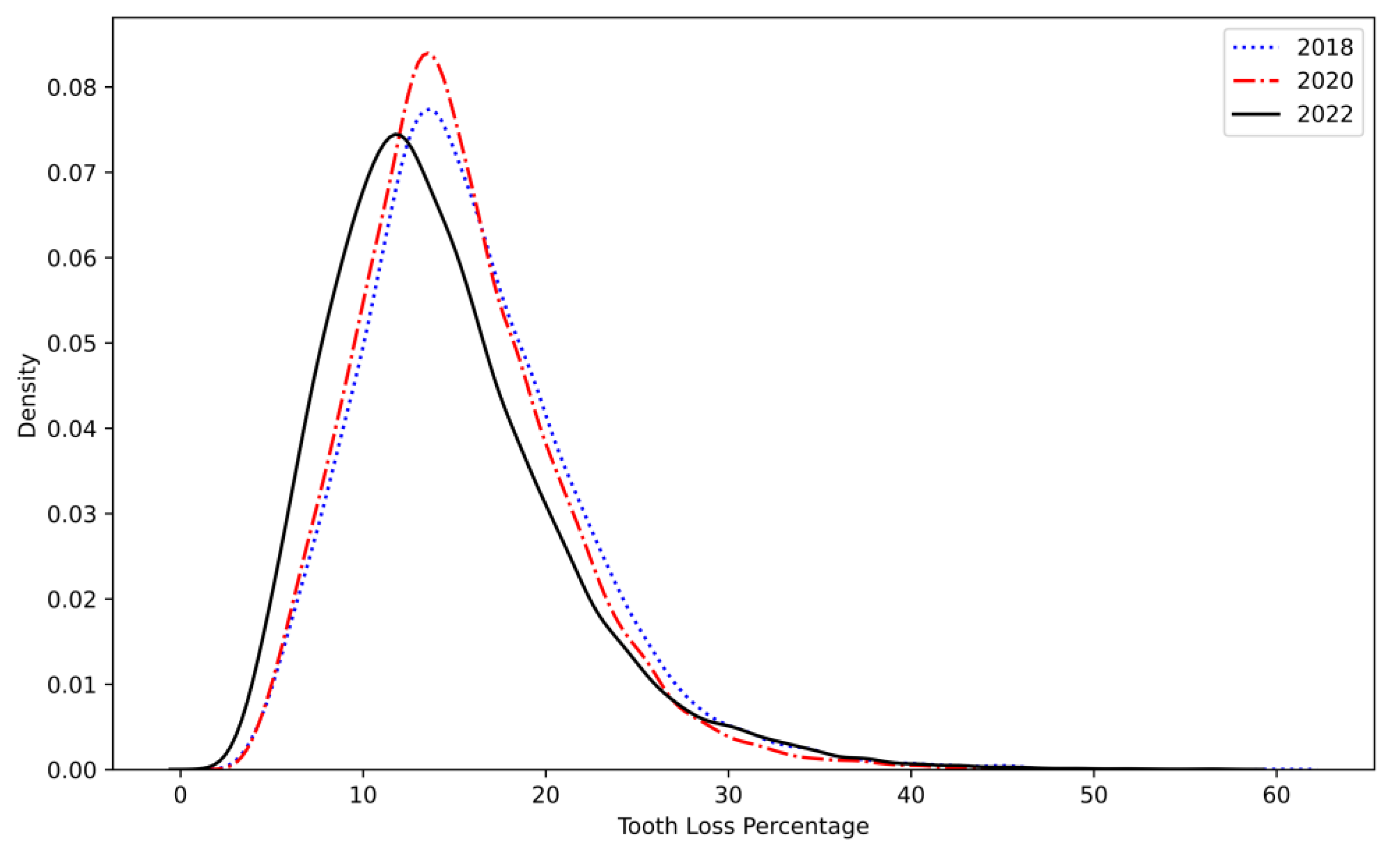
Figure 2.
Hot Spot Analysis (Getis-Ord Gi) of Tooth Loss Prevalence in 2018. * The figure represents the spatial distribution of tooth loss prevalence among older adults in 2018 based on the Getis-Ord Gi* statistic. ZCTAs are classified into four categories: The map uses four color codes to show prevalence levels: black for high prevalence areas and red for moderate prevalence areas with orange indicating low prevalence and pale yellow showing very low prevalence. Regions with significantly higher tooth loss rates form hot spots mostly located in the Southeast and Midwest areas while cold spots appear more frequently across the Northeast and West Coast.
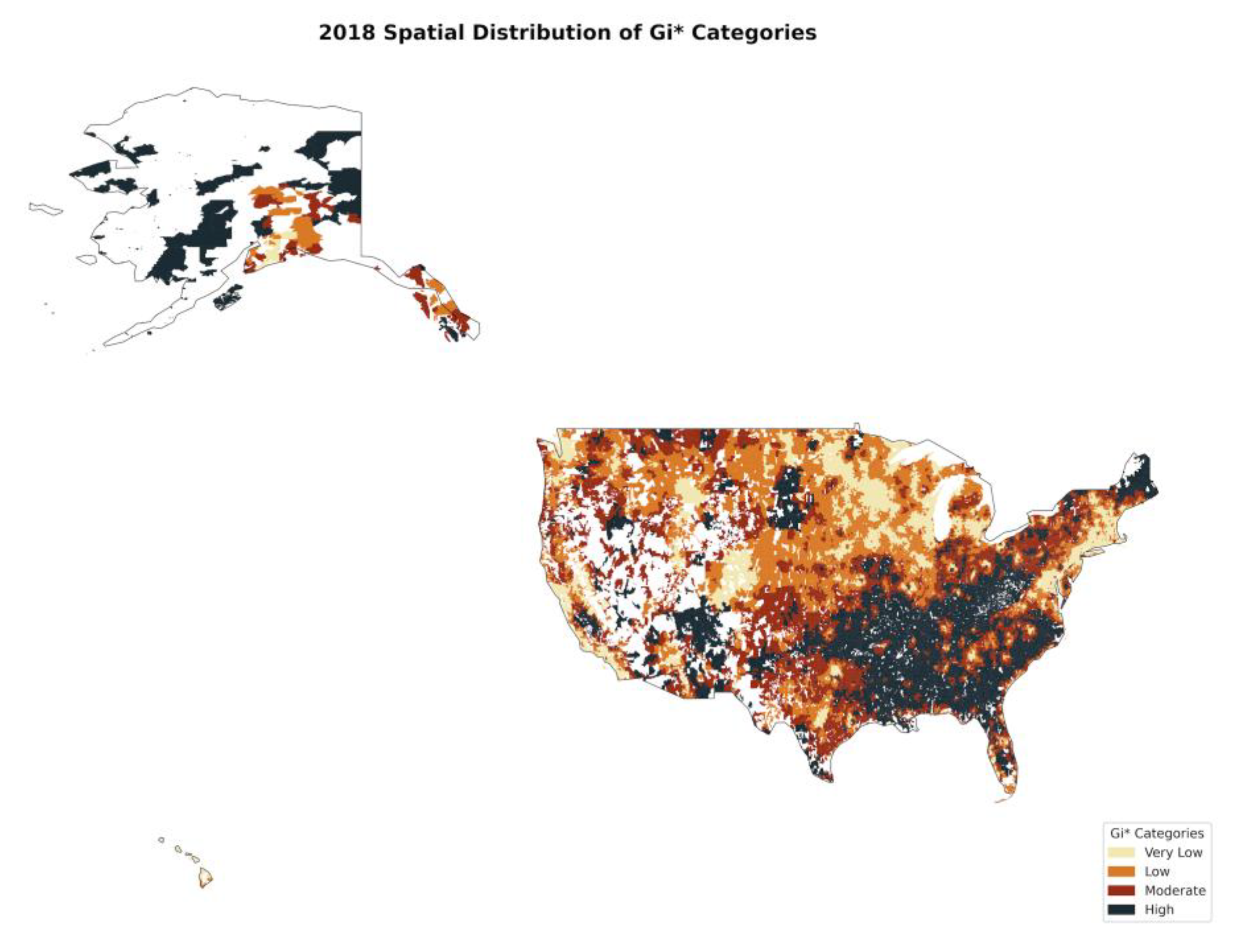
Figure 3.
Hot Spot Analysis (Getis-Ord Gi) of Tooth Loss Prevalence in 2020. * The shown figure represents the geographic spread of tooth loss rates in 2020 using Getis-Ord Gi* analysis. The geographic range of hot spots reached further into the Midwest and Southern U.S. in comparison to 2018, while cold spots reduced, especially in urban regions. The COVID-19 pandemic disrupted access to dental care which appears to be causing an increase in disparities.
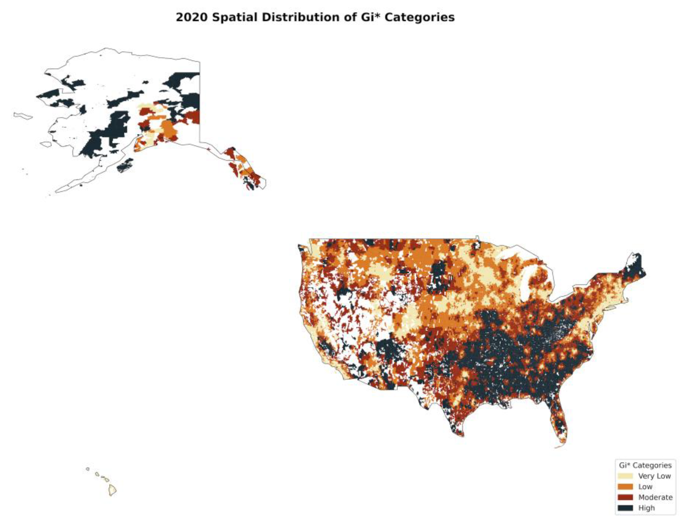
Figure 4.
Hot Spot Analysis (Getis-Ord Gi) of Tooth Loss Prevalence in 2022. * The figure depicts how tooth loss prevalence clusters geographically for the year 2022. Some urban areas have demonstrated recovery through the reemergence of cold spots, yet high-prevalence clusters continue to persist in the Southeast and rural areas. The continued presence of high tooth loss areas demonstrates how structural barriers and socioeconomic inequality affect oral healthcare availability for elderly populations.

Table 1.
Ordinary Least Squares (OLS) Regression Results Without Interaction Terms.
| Model Fit Statistics | Value | |||||
| Dependent variable | Total tooth loss (≥65 years, %) | |||||
| Number of observations | 89380 | |||||
| R2 | 0.609 | |||||
| Adjusted R2 | 0.609 | |||||
| F-statistic | 9943 | |||||
| Prob (F-statistic) | <0.001 | |||||
| Log-likelihood | -246200 | |||||
| AIC | 492437 | |||||
| BIC | 492578 | |||||
| Durbin–Watson statistic | 1.414 | |||||
| Breusch–Godfrey LM statistic | 7841 | |||||
| Breusch–Godfrey p-value | <0.001 | |||||
| Variable | Coef | Std Err | t | P>|t| | 95% CI | VIF |
| Contstant | 28.545 | 0.145 | 196.304 | <0.001 | [28.26, 28.83] | 162.213 |
| Percent Uninsured (>=65 years) | 0.042 | 0.006 | 7.033 | <0.001 | [0.03, 0.054] | 1.079 |
| High school graduate or higher (>=65 Years) | -0.112 | 0.001 | -87.952 | <0.001 | [-0.114, -0.109] | 2.475 |
| Bachelor's degree or higher (6>=5 Years) | -0.131 | 0.001 | -93.914 | <0.001 | [-0.134, -0.128] | 3.196 |
| Population Percentage (>=65 years) | -0.149 | 0.003 | -44.157 | <0.001 | [-0.155, -0.142] | 5.435 |
| Number of individuals (>=65 years) per housing unit | 5.522 | 0.161 | 34.383 | <0.001 | [5.207, 5.837] | 5.141 |
| Monthly Housing Costs in ZCTA | -0.0030 | 0.000 | -62.706 | <0.001 | [-0.003, -0.003] | 3.888 |
| Median income in ZCTA | -0.0000656 | 0.000 | -73.018 | <0.001 | [-0.0000674, -0.0000638] | 3.989 |
| Percent below poverty level (>=65 years) | 0.072 | 0.002 | 43.841 | <0.001 | [0.069, 0.076] | 1.307 |
| Female Percentage (>=65 years) | 0.00140 | 0.001 | 0.990 | 0.322 | [-0.001, 0.004] | 1.036 |
| Year_Dummy_2020 (referenced 2018) | 0.093 | 0.031 | 2.980 | 0.003 | [0.032, 0.155] | 1.345 |
| Year_Dummy_2022 (referenced 2018) | 0.452 | 0.033 | 13.880 | <0.001 | [0.388, 0.515] | 1.447 |
| White_Majority Zipcode (>=65 years) | 2.882 | 0.089 | 32.349 | <0.001 | [2.707, 3.056] | 4.474 |
| Black_Majority Zipcode (>=65 years) | 7.481 | 0.105 | 70.929 | <0.001 | [7.274, 7.687] | 3.020 |
| Other_Majority Zipcode (>=65 years) | 7.302 | 0.124 | 58.764 | <0.001 | [7.058, 7.545] | 2.386 |
* Notes: Ordinary least squares estimates are reported with non-robust standard errors. Year indicators use 2018 as the reference category. ZCTA denotes Zip Code Tabulation Area.
Table 2.
Ordinary Least Squares (OLS) Regression Results With Interaction Terms.
| Model Fit Statistics | Value | ||||||
| Dependent variable | Total tooth loss (≥65 years, %) | ||||||
| Number of observations | 89380 | ||||||
| R2 | 0.596 | ||||||
| Adjusted R2 | 0.596 | ||||||
| F-statistic | 7769 | ||||||
| Prob (F-statistic) | <0.001 | ||||||
| Log-likelihood | -247910 | ||||||
| AIC | 495268 | ||||||
| BIC | 495437 | ||||||
| Durbin–Watson statistic | 1.402 | ||||||
| Breusch–Godfrey LM statistic | 8128 | ||||||
| Breusch–Godfrey p-value | <0.001 | ||||||
| Variable | Coef | Std Err | t | P>|t| | 95% CI | VIF | |
| Constant | 31.62 | 0.14 | 229.90 | <0.001 | [31.35, 31.89] | 113.31 | |
| Percent Uninsured (>=65 years) | 0.04 | 0.01 | 6.98 | <0.001 | [0.03, 0.05] | 1.07 | |
| High school graduate or higher (>=65 Years) | -0.11 | 0.00 | -89.60 | <0.001 | [-0.12, -0.11] | 2.36 | |
| Bachelor's degree or higher (6>=5 Years) | -0.13 | 0.00 | -94.14 | <0.001 | [-0.13, -0.13] | 3.10 | |
| Population Percentage (>=65 years) | -0.15 | 0.00 | -44.75 | <0.001 | [-0.16, -0.15] | 5.41 | |
| Number of individuals (>=65 years) per housing unit | 5.60 | 0.16 | 34.35 | <0.001 | [5.28, 5.92] | 5.12 | |
| Monthly Housing Costs in ZCTA | -0.003 | 0.00 | -60.81 | <0.001 | [-0.003, -0.004] | 3.86 | |
| Median income in ZCTA | -0.0000673 | 0.00 | -74.02 | <0.001 | [-0.0000691, -0.0000656] | 3.96 | |
| Percent below poverty level (>=65 years) | 0.08 | 0.00 | 46.30 | <0.001 | [0.07, 0.08] | 1.30 | |
| Female Percentage (>=65 years) | 0.0033 | 0.00 | 2.38 | 0.020 | [0.001, 0.006] | 1.03 | |
| Year_Dummy_2020 (referenced 2018) | -3.08 | 0.15 | -21.16 | <0.001 | [-3.37, -2.8] | 28.25 | |
| Year_Dummy_2022 (referenced 2018) | -2.26 | 0.14 | -15.95 | <0.001 | [-2.54, -1.98] | 26.54 | |
| Interactive_year_2020_with_White_Majority (referenced to 2018, Hispanic) | 3.06 | 0.15 | 20.83 | <0.001 | [2.77, 3.35] | 27.41 | |
| Interactive_year_2020_with_Black_Majority (referenced to 2018, Hispanic) | 7.11 | 0.18 | 38.89 | <0.001 | [6.75, 7.47] | 2.50 | |
| Interactive_year_2020_with_Other_Majority (referenced to 2018, Hispanic) | 6.10 | 0.22 | 28.20 | <0.001 | [5.67, 6.52] | 1.74 | |
| Interactive_year_2022_with_White_Majority (referenced to 2018, Hispanic) | 2.51 | 0.14 | 17.60 | <0.001 | [2.23, 2.79] | 25.75 | |
| Interactive_year_2022_with_Black_Majority (referenced to 2018, Hispanic) | 7.53 | 0.180 | 41.92 | <0.001 | [7.18, 7.89] | 2.41 | |
| Interactive_year_2022_with_Other_Majority (referenced to 2018, Hispanic) | 7.45 | 0.21 | 34.99 | <0.001 | [7.03, 7.87] | 1.71 | |
Table 3.
Moran’s I Test for Spatial Autocorrelation of Tooth Loss (2018-2022).
| Year | Moran’s I | p-value | Z-score | Interpretation |
| 2018 | 0.71 | 0.00 | 205.27 | Strong spatial clustering |
| 2020 | 0.71 | 0.00 | 212.74 | Strong spatial clustering (slightly lower than 2018) |
| 2022 | 0.63 | 0.00 | 184.59 | Strong but weaker clustering than previous years |
Table 4.
Spatial Lag Model (SLM) Results for 2018.
| Model Fit Statistics | Value | |||
| AIC: | 150788.770 | |||
| Schwarz criterion | 150871.537 | |||
| Pseudo R-squared | 0.719 | |||
| Spatial Pseudo R-squared | 0.613 | |||
| Variable | Coefficient | Std Err | z-Statistic | Probability |
| Constant | 22.596 | 0.205 | 110.017 | <0.001 |
| Percent Uninsured (>=65 years) | 0.029 | 0.010 | 2.991 | 0.003 |
| High school graduate or higher (>=65 Years) | -0.083 | 0.002 | -43.711 | <0.001 |
| Bachelor's degree or higher (>=65 Years) | -0.097 | 0.002 | -45.893 | <0.001 |
| Percentage of Population (>=65 years) | -0.151 | 0.006 | -25.314 | <0.001 |
| Number of individuals (>=65 years) per housing unit | 5.383 | 0.286 | 18.832 | <0.001 |
| Monthly Housing Costs in ZCTA | -0.001 | 0.000 | -12.215 | <0.001 |
| Median income in ZCTA | 0.000 | 0.000 | -52.622 | <0.001 |
| Percent below poverty level (>=65 years) | 0.071 | 0.003 | 25.968 | <0.001 |
| Coefficient for the spatially lag | 0.062 | 0.001 | 89.047 | <0.001 |
| Variable | Direct | Indirect | Total | |
| Percent Uninsured (>=65 years) | 0.029 | 0.002 | 0.031 | |
| High school graduate or higher (>=65 Years) | -0.083 | -0.006 | -0.089 | |
| Bachelor's degree or higher (>=65 Years) | -0.097 | -0.006 | -0.104 | |
| Percentage of Population (>=65 years) | -0.151 | -0.010 | -0.161 | |
| Number of individuals (>=65 years) per housing unit | 5.383 | 0.354 | 5.737 | |
| Monthly Housing Costs in ZCTA | -0.001 | 0.000 | -0.001 | |
| Median income in ZCTA | 0.000 | 0.000 | 0.000 | |
| Percent below poverty level (>=65 years) | 0.071 | 0.005 | 0.076 |
Table 5.
Spatial Lag Model (SLM) Results for 2020.
| Model Fit Statistics | Value | |||
| AIC: | 143482.792 | |||
| Schwarz criterion | 143565.765 | |||
| Pseudo R-squared | 0.787 | |||
| Spatial Pseudo R-squared | 0.636 | |||
| Variable | Coefficient | Std Err | z-Statistic | Probability |
| Constant | 5.415 | 0.067 | 80.647 | <0.001 |
| Percent Uninsured (>=65 years) | 0.114 | 0.016 | 7.323 | <0.001 |
| High school graduate or higher (>=65 Years) | -0.752 | 0.023 | -32.559 | <0.001 |
| Bachelor's degree or higher (>=65 Years) | -1.041 | 0.027 | -39.201 | <0.001 |
| Percentage of Population (>=65 years) | -0.742 | 0.036 | -20.776 | <0.001 |
| Number of individuals (>=65 years) per housing unit | 0.496 | 0.035 | 14.342 | <0.001 |
| Monthly Housing Costs in ZCTA | -0.195 | 0.030 | -6.450 | <0.001 |
| Median income in ZCTA | -1.384 | 0.029 | -47.980 | <0.001 |
| Percent below poverty level (>=65 years) | 0.426 | 0.017 | 25.027 | <0.001 |
| Coefficient for the spatially lag | 0.645 | 0.004 | 150.326 | <0.001 |
| Variable | Direct | Indirect | Total | |
| Percent Uninsured (>=65 years) | 0.114 | 0.207 | 0.321 | |
| High school graduate or higher (>=65 Years) | -0.752 | -1.367 | -2.118 | |
| Bachelor's degree or higher (>=65 Years) | -1.041 | -1.893 | -2.935 | |
| Percentage of Population (>=65 years) | -0.742 | -1.350 | -2.092 | |
| Number of individuals (>=65 years) per housing unit | 0.497 | 0.903 | 1.399 | |
| Monthly Housing Costs in ZCTA | -0.195 | -0.355 | -0.550 | |
| Median income in ZCTA | -1.384 | -2.516 | -3.900 | |
| Percent below poverty level (>=65 years) | 0.426 | 0.774 | 1.200 |
Table 6.
Spatial Lag Model (SLM) Results for 2022.
| Model Fit Statistics | Value | |||
| AIC: | 153663.559 | |||
| Schwarz criterion | 153746.171 | |||
| Pseudo R-squared | 0.707 | |||
| Spatial Pseudo R-squared | 0.587 | |||
| Variable | Coefficient | Std Err | z-Statistic | Probability |
| Constant | 16.038 | 0.248 | 64.733 | <0.001 |
| Percent Uninsured (>=65 years) | 0.045 | 0.010 | 4.536 | <0.001 |
| High school graduate or higher (>=65 Years) | -0.062 | 0.002 | -28.541 | <0.001 |
| Bachelor's degree or higher (>=65 Years) | -0.079 | 0.002 | -33.381 | <0.001 |
| Percentage of Population (>=65 years) | -0.119 | 0.006 | -20.977 | <0.001 |
| Number of individuals (>=65 years) per housing unit | 4.096 | 0.269 | 15.252 | <0.001 |
| Monthly Housing Costs in ZCTA | 0.000 | 0.000 | -2.259 | 0.024 |
| Median income in ZCTA | 0.000 | 0.000 | -44.291 | <0.001 |
| Percent below poverty level (>=65 years) | 0.071 | 0.003 | 25.845 | <0.001 |
| Coefficient for the spatially lag | 0.571 | 0.005 | 110.270 | <0.001 |
| Variable | Direct | Indirect | Total | |
| Percent Uninsured (>=65 years) | 0.045 | 0.060 | 0.105 | |
| High school graduate or higher (>=65 Years) | -0.062 | -0.082 | -0.144 | |
| Bachelor's degree or higher (>=65 Years) | -0.079 | -0.105 | -0.184 | |
| Percentage of Population (>=65 years) | -0.119 | -0.158 | -0.277 | |
| Number of individuals (>=65 years) per housing unit | 4.096 | 5.455 | 9.552 | |
| Monthly Housing Costs in ZCTA | 0.000 | 0.000 | 0.000 | |
| Median income in ZCTA | 0.000 | 0.000 | 0.000 | |
| Percent below poverty level (>=65 years) | 0.071 | 0.094 | 0.165 |
Table 7.
Spatial Error Model (SEM) Results for 2018.
| Model Fit Statistics | Value | |||
| AIC: | 142360 | |||
| Schwarz criterion | 142434 | |||
| Mean dependent var | 16 | |||
| S.D. dependent var | 6 | |||
| Pseudo R-squared | 1 | |||
| Log likelihood | -71171 | |||
| Sigma-square ML | 7 | |||
| S.E of regression | 3 | |||
| Variable | Coefficient | Std Err | z-Statistic | Probability |
| Constant | 26.707 | 0.174 | 153.386 | <0.001 |
| Percent Uninsured (>=65 years) | 0.049 | 0.008 | 6.174 | <0.001 |
| High school graduate or higher (>=65 Years) | -0.053 | 0.002 | -30.723 | <0.001 |
| Bachelor's degree or higher (>=65 Years) | -0.073 | 0.002 | -36.992 | <0.001 |
| Percentage of Population (>=65 years) | -0.149 | 0.005 | -29.225 | <0.001 |
| Number of individuals (>=65 years) per housing unit | 5.408 | 0.247 | 21.866 | <0.001 |
| Monthly Housing Costs in ZCTA | -0.002 | 0.000 | -20.553 | <0.001 |
| Median income in ZCTA | 0.000 | 0.000 | -50.086 | <0.001 |
| Percent below poverty level (>=65 years) | 0.058 | 0.002 | 25.983 | <0.001 |
| Lambda | 0.795 | 0.004 | 178.992 | <0.001 |
Table 8.
Spatial Error Model (SEM) Results for 2020.
| Model Fit Statistics | Value | |||
| AIC: | 144176 | |||
| Schwarz criterion | 144251 | |||
| Mean dependent var | 15 | |||
| S.D. dependent var | 6 | |||
| Pseudo R-squared | 1 | |||
| Log likelihood | -72079 | |||
| Sigma-square ML | 7 | |||
| S.E of regression | 3 | |||
| Variable | Coefficient | Std Err | z-Statistic | Probability |
| Constant | 24.999 | 0.161 | 155.488 | <0.001 |
| Percent Uninsured (>=65 years) | 0.041 | 0.007 | 6.289 | <0.001 |
| High school graduate or higher (>=65 Years) | -0.041 | 0.002 | -26.779 | <0.001 |
| Bachelor's degree or higher (>=65 Years) | -0.063 | 0.002 | -35.792 | <0.001 |
| Percentage of Population (>=65 years) | -0.093 | 0.004 | -22.931 | <0.001 |
| Number of individuals (>=65 years) per housing unit | 2.852 | 0.197 | 14.501 | <0.001 |
| Monthly Housing Costs in ZCTA | -0.003 | 0.000 | -30.549 | <0.001 |
| Median income in ZCTA | 0.000 | 0.000 | -43.063 | <0.001 |
| Percent below poverty level (>=65 years) | 0.040 | 0.002 | 21.512 | <0.001 |
| Lambda | 0.788 | 0.004 | 175.568 | <0.001 |
Table 9.
Spatial Error Model (SEM) Results for 2022.
| Model Fit Statistics | Value | |||
| AIC: | 154568 | |||
| Schwarz criterion | 154642 | |||
| Mean dependent var | 14 | |||
| S.D. dependent var | 6 | |||
| Pseudo R-squared | 1 | |||
| Log likelihood | -77275 | |||
| Sigma-square ML | 12 | |||
| S.E of regression | 3 | |||
| Variable | Coefficient | Std Err | z-Statistic | Probability |
| Constant | 26.843 | 0.230 | 116.531 | <0.001 |
| Percent Uninsured (>=65 years) | 0.055 | 0.010 | 5.551 | <0.001 |
| High school graduate or higher (>=65 Years) | -0.059 | 0.002 | -24.919 | <0.001 |
| Bachelor's degree or higher (>=65 Years) | -0.085 | 0.003 | -32.351 | <0.001 |
| Percentage of Population (>=65 years) | -0.132 | 0.006 | -22.589 | <0.001 |
| Number of individuals (>=65 years) per housing unit | 4.134 | 0.279 | 14.844 | <0.001 |
| Monthly Housing Costs in ZCTA | -0.002 | 0.000 | -20.115 | <0.001 |
| Median income in ZCTA | 0.000 | 0.000 | -41.864 | <0.001 |
| Percent below poverty level (>=65 years) | 0.058 | 0.003 | 21.287 | <0.001 |
| Lambda | 0.683 | 0.006 | 118.410 | <0.001 |
Table 10.
Geographically Weighted Regression (GWR) Results for 2018.
| Model Fit Statistics | Global Regression | GWR | |||
| AIC: | 158960 | 132322 | |||
| AICc: | 158962 | 135334 | |||
| BIC: | 106130 | 181177 | |||
| R2: | 0.618 | 0.898 | |||
| Adjusted R2 | 0.618 | 0.872 | |||
| Variable | Mean | STD | Min | Median | Max |
| Intercept | 14.808 | 2.281 | 0.829 | 14.877 | 29.156 |
| Percent Uninsured (>=65 years) | 0.168 | 0.929 | -14.623 | 0.106 | 7.144 |
| High school graduate or higher (>=65 Years) | -0.991 | 1.096 | -6.024 | -0.832 | 3.758 |
| Bachelor's degree or higher (>=65 Years) | -1.328 | 1.247 | -6.487 | -1.191 | 3.990 |
| Percentage of Population (>=65 years) | -2.076 | 2.183 | -15.626 | -1.661 | 7.510 |
| Number of individuals (>=65 years) per housing unit | 1.546 | 1.870 | -7.237 | 1.247 | 10.639 |
| Monthly Housing Costs in ZCTA | -1.402 | 2.226 | -17.471 | -1.269 | 8.653 |
| Median income in ZCTA | -2.651 | 1.803 | -11.835 | -2.351 | 4.888 |
| Percent below poverty level (>=65 years) | 0.643 | 0.779 | -2.827 | 0.523 | 4.540 |
Table 11.
Geographically Weighted Regression (GWR) Results for 2020.
| Model Fit Statistics | Global Regression | GWR | |||
| AIC: | 159588 | 136157 | |||
| AICc: | 159590 | 139076 | |||
| BIC: | 72008 | 185014 | |||
| R2: | 0.598 | 0.877 | |||
| Adjusted R2 | 0.598 | 0.847 | |||
| Variable | Mean | STD | Min | Median | Max |
| Intercept | 14.526 | 2.169 | 2.727 | 14.478 | 26.317 |
| Percent Uninsured (>=65 years) | 0.255 | 1.142 | -19.818 | 0.134 | 17.001 |
| High school graduate or higher (>=65 Years) | -0.992 | 1.184 | -8.729 | -0.802 | 2.588 |
| Bachelor's degree or higher (>=65 Years) | -1.346 | 1.329 | -9.424 | -1.215 | 3.077 |
| Percentage of Population (>=65 years) | -1.578 | 1.964 | -14.644 | -1.241 | 4.887 |
| Number of individuals (>=65 years) per housing unit | 1.083 | 1.651 | -4.494 | 0.809 | 10.064 |
| Monthly Housing Costs in ZCTA | -1.634 | 1.864 | -18.698 | -1.456 | 5.306 |
| Median income in ZCTA | -2.040 | 1.502 | -10.418 | -1.794 | 4.730 |
| Percent below poverty level (>=65 years) | 0.602 | 0.793 | -1.867 | 0.456 | 4.270 |
Table 12.
Geographically Weighted Regression (GWR) Results for 2022.
| Model Fit Statistics | Global Regression | GWR | |||
| AIC: | 163614 | 147509 | |||
| AICc: | 163616 | 149226 | |||
| BIC: | 217169 | 185050 | |||
| R2: | 0.555 | 0.816 | |||
| Adjusted R2 | 0.555 | 0.781 | |||
| Variable | Mean | STD | Min | Median | Max |
| Intercept | 13.360 | 2.012 | 6.224 | 13.390 | 25.118 |
| Percent Uninsured (>=65 years) | 0.208 | 0.845 | -5.720 | 0.154 | 7.092 |
| High school graduate or higher (>=65 Years) | -1.088 | 1.261 | -7.173 | -0.947 | 4.091 |
| Bachelor's degree or higher (>=65 Years) | -1.488 | 1.399 | -8.192 | -1.407 | 5.952 |
| Percentage of Population (>=65 years) | -1.916 | 2.090 | -13.552 | -1.567 | 4.230 |
| Number of individuals (>=65 years) per housing unit | 1.358 | 1.832 | -6.463 | 1.134 | 11.637 |
| Monthly Housing Costs in ZCTA | -1.521 | 2.147 | -12.023 | -1.334 | 6.770 |
| Median income in ZCTA | -2.612 | 1.868 | -10.920 | -2.234 | 3.068 |
| Percent below poverty level (>=65 years) | 0.721 | 0.856 | -1.712 | 0.614 | 4.334 |
Table 13.
Summary of Spatial Lag Model Performance & Socioeconomic Effects Over Time.
| Variable | 2018 | 2020 | 2022 | Trend & Interpretation |
| Pseudo R² | 0.719 | 0.787 | 0.707 | Best model fit in 2020, slight decline in 2022. |
| Spatial Pseudo R² | 0.613 | 0.636 | 0.587 | Spatial dependence strongest in 2020, weaker in 2022. |
| AIC (Model Fit) | 150789 | 143483 | 153664 | Best model fit in 2020, worsened in 2022. |
| Spatial Lag Coefficient (ρ) | 0.062 | 0.645 | 0.571 | Spatial dependence peaked in 2020, then weakened. |
| Percent Uninsured (>=65 years) | 0.031 | 0.321 | 0.105 | Huge impact in 2020 due to COVID-related healthcare access issues. Decreased in 2022 but still significant. |
| High School Graduate (>=65 years) | -0.089 | -2.118 | -0.144 | Biggest impact in 2020, possibly due to disparities in access to dental care. Stabilized in 2022. |
| Bachelor’s Degree or Higher (>=65 years) | -0.104 | -2.935 | -0.184 | Strongest effect in 2020, weakened in 2022 but still significant. |
| Population (>=65 years) | -0.161 | -2.092 | -0.277 | Aging population had the most impact in 2020, but spatial spillover reduced in 2022. |
| Individuals per Housing Unit (>=65 years) | 5.737 | 1.399 | 9.552 | Strongest impact in 2022, suggesting household crowding effects worsened post-COVID. |
| Monthly Housing Costs | -0.001 | -0.550 | 0.000 | Had a stronger effect in 2020, possibly due to economic hardships during the pandemic. |
| Median Income in ZCTA | 0.000 | -3.900 | 0.000 | Income disparities peaked in 2020 but had little impact in 2022, suggesting a shift in determinants of tooth loss. |
| Percent Below Poverty (>=65 years) | 0.076 | 1.200 | 0.165 | Poverty had the highest effect in 2020, but still strongly contributes to disparities in 2022. |
*Notes: Comparison of model fit statistics, spatial dependence, and direct/indirect effects of key socioeconomic factors on tooth loss from 2018-2022.
Table 14.
Summary of Spatial Error Model (SEM) Performance and Interpretation of Coefficients.
| Variable | 2018 SEM | 2020 SEM | 2022 SEM | Trend & Interpretation |
| AIC | 142360 | 144176 | 154568 | Model fit worsened in 2022, suggesting new unobserved influences on tooth loss. |
| Schwarz Criterion (BIC) | 142434 | 144251 | 154642 | Consistent trend. |
| Pseudo R² | 0.610 | 0.587 | 0.546 | Explanatory power declined, suggesting stronger spatial heterogeneity over time. |
| Log Likelihood | -71171 | -72079 | -77275 | Model fit degraded over time, likely due to shifting regional disparities. |
| Sigma-Square ML | 6.753 | 6.522 | 11.746 | Error variance increased significantly in 2022, meaning more unexplained variation. |
| S.E. of Regression | 2.599 | 2.554 | 3.427 | Greater residual variability in 2022, meaning larger differences in regional effects. |
| Percent Uninsured (>=65 years) | 0.049 | 0.041 | 0.055 | Rebounded in 2022, suggesting access to healthcare still varies regionally. |
| High School Graduate (>=65 years) | -0.053 | -0.041 | -0.059 | Education’s impact increased in 2022, reinforcing its importance in oral health. |
| Bachelor’s Degree or Higher (>=65 years) | -0.073 | -0.063 | -0.085 | Higher education had the strongest effect in 2022, likely due to better self-care and healthcare access. |
| Population (>=65 years) | -0.149 | -0.093 | -0.132 | Stronger protective effect in 2018, weakened in 2020, but partially rebounded in 2022. |
| Individuals per Housing Unit (>=65 years) | 5.408 | 2.852 | 4.134 | Crowding had the strongest effect in 2018, was weaker in 2020, and rebounded in 2022 as economic stressors persisted. |
| Monthly Housing Costs in ZCTA | -0.002 | -0.003 | -0.002 | Weaker effect in 2022, suggesting housing affordability had a diminished role. |
| Median Income in ZCTA | 0.000 | 0.000 | 0.000 | Stable effect, meaning income remained a key protective factor. |
| Percent Below Poverty (>=65 years) | 0.058 | 0.040 | 0.058 | Worsened in 2022, meaning economic disparities continued to drive tooth loss inequalities. |
| Lambda (Spatial Error Term) | 0.795 | 0.788 | 0.683 | Spatial autocorrelation weakened in 2022, meaning unobserved geographic factors are less dominant now. |
*Notes: Evaluation of SEM results across years, indicating changes in explanatory power, model fit, and spatial heterogeneity.
Table 15.
Geographically Weighted Regression (GWR) Model Performance and Interpretation of Coefficients (2018-2022).
Table 15.
Geographically Weighted Regression (GWR) Model Performance and Interpretation of Coefficients (2018-2022).
| Metric | 2018 GWR | 2020 GWR | 2022 GWR | Trend & Interpretation |
| R² | 0.898 | 0.877 | 0.816 | Model fit was highest in 2018, but declined over time, likely due to external disruptions (e.g., COVID-19, policy shifts). |
| Adjusted R² | 0.872 | 0.847 | 0.781 | Suggests increasing external influences affecting disparities. (e.g., policy changes, economic shifts). |
| AIC | 132322 | 136157 | 147509 | Best model fit in 2018, worsened over time, indicating changing patterns in disparities. |
| BIC | 181177 | 185014 | 185050 | Model complexity increased slightly, especially post-2020. |
| Percent Uninsured (>=65 years) | 0.168 | 0.255 | 0.208 | Uninsured seniors had the strongest impact on tooth loss in 2020 (COVID-19 impact). The effect weakened in 2022 as healthcare access recovered. |
| High School Graduate (>=65 years) | -0.991 | -0.992 | -1.088 | Consistently reduces tooth loss, with a slightly stronger effect in 2022. Education remained a key protective factor. |
| Bachelor’s Degree or Higher (>=65 years) | -1.328 | -1.346 | -1.488 | Higher education consistently reduced tooth loss, with the strongest effect in 2022. Likely due to greater awareness and access to dental care. |
| Population (>=65 years) | -2.076 | -1.578 | -1.916 | Aging population showed the strongest protective effect in 2018, weakened in 2020, but slightly recovered in 2022. |
| Individuals per Housing Unit (>=65 years) | 1.546 | 1.083 | 1.358 | Crowding became a weaker predictor in 2020 but rebounded in 2022, suggesting persistent economic stress in some areas. |
| Monthly Housing Costs in ZCTA | -1.402 | -1.634 | -1.521 | Stronger effect in 2020, indicating economic pressures during COVID-19, slightly weaker in 2022. |
| Median Income in ZCTA | -2.651 | -2.040 | -2.612 | Income had the strongest impact in 2018, weakened in 2020 (possibly due to pandemic shocks), then partially recovered in 2022. |
| Percent Below Poverty (>=65 years) | 0.643 | 0.602 | 0.721 | Poverty consistently worsened tooth loss, with the strongest effect in 2022. Suggests long-term economic disparities worsened post-pandemic. |
*Notes: The performance metrics and key coefficients from the Geographically Weighted Regression (GWR) models for total tooth loss prevalence among the geriatric population across U.S. ZCTAs for the years 2018, 2020, and 2022.
Table 16.
Hot Spot Analysis (Getis-Ord Gi) – Key Trends in Tooth Loss Clustering (2018-2022).
| Year | Hot Spots (High Tooth Loss) | Cold Spots (Low Tooth Loss) | Interpretation |
| 2018 | Concentrated in the Southeast, Appalachia, and Midwest. | Strongest in the West Coast, Northeast, and urban centers. | Structural disparities were already in place. |
| 2020 | Expanded into Midwest, Texas, and urban areas. | Shrunk significantly, especially in previously stable regions. | Pandemic worsened disparities and disrupted dental care access. |
| 2022 | Remained strong in Southern and rural regions. | Some recovery in urban and high-income areas. | Post-pandemic, disparities remained, with long-term factors driving the trends. |
* Note: Summary of spatial clustering trends, showing the evolution of high-prevalence (hot spots) and low-prevalence (cold spots) regions across study years.
Disclaimer/Publisher’s Note: The statements, opinions and data contained in all publications are solely those of the individual author(s) and contributor(s) and not of MDPI and/or the editor(s). MDPI and/or the editor(s) disclaim responsibility for any injury to people or property resulting from any ideas, methods, instructions or products referred to in the content. |
© 2026 by the authors. Licensee MDPI, Basel, Switzerland. This article is an open access article distributed under the terms and conditions of the Creative Commons Attribution (CC BY) license (http://creativecommons.org/licenses/by/4.0/).
Copyright: This open access article is published under a Creative Commons CC BY 4.0 license, which permit the free download, distribution, and reuse, provided that the author and preprint are cited in any reuse.


