Submitted:
02 February 2026
Posted:
06 February 2026
You are already at the latest version
Abstract
We derive eigenvalue bounds for symmetric block-tridiagonal multiple saddle-point systems preconditioned with the symmetric positive definite (SPD) preconditioner proposed by J. Pearson and A. Potschka in 2024, and further studied by L. Bergamaschi and coauthors, for double saddle point problems, with inexact Schur complement matrices. The analysis applies to an arbitrary number of blocks. Numerical experiments are carried out to validate the proposed estimates.
Keywords:
multiple saddle-point systems
; preconditioned iterative methods
; symmetric positive definite preconditioner
; eigenvalue bounds
1. Introduction
We consider the iterative solution of a block tridiagonal multiple saddle-point linear system , where
We assume that is symmetric positive definite, all other square block matrices are symmetric positive semi-definite and have full rank (for ). We assume also that for all k. These conditions are sufficient to ensure the invertibility of .
Linear systems involving matrix arise mostly with (double saddle–point systems) in many scientific applications including magma–mantle dynamics [3], liquid crystal director modeling [4] or in the coupled Stokes–Darcy problem [5,6,7,8], and the preconditioning of such linear systems has been considered in [9,10,11]. In particular, block diagonal preconditioners for matrix have been studied in [12,13,14,15,16].
Multiple saddle-point linear systems with have recently attracted the attention of a number of researchers. Such systems often arise from modeling multiphysics processes, i.e. the simultaneous simulation of different aspects of physical systems and the interactions among them. Preconditioning of the saddle-point linear system (), although with a different block structure, has been addressed in [17] to solve a class of optimal control problems. A practical preconditioning strategy for multiple saddle–point linear systems, based on sparse approximate inverses of the diagonal blocks of the block diagonal Schur complement preconditioning matrix, is proposed in [18], for the solution of coupled poromechanical models and the mechanics of fractured media. Theoretical analysis of such preconditioners has been carried on in [19]. In [17], two multiple saddle-point systems arising from optimal control problems constrained with either the heat or the wave equation are addressed, and iteratively solved by robust block diagonal preconditioners.
In this work we consider the preconditioner proposed in [1] (PP preconditioner in short) to develop a spectral analysis of the preconditioned matrix for an arbitrary number of blocks and in presence of inexact Schur complements, in the line of [15] in which the block diagonal preconditioner with exact Schur complements is considered. We will define a sequence of polynomials by a three-term recurrence, whose extremal roots characterize the eigenvalues of the preconditioned matrix in terms of the nonnegative eigenvalues of the preconditioned Schur complements. Using a similar technique, we will extend results, obtained in [2] for a double saddle-point, to multiple saddle-point linear system.
Arguably the most prominent Krylov subspace methods for solving the linear system are preconditioned variants of MINRES [20] and GMRES [21]. In contrast to GMRES, the previously-discovered MINRES algorithm can explicitly exploit the symmetry of . As a consequence, MINRES features a three-term recurrence relation, which is beneficial for its implementation (low memory requirements because subspace bases need not be stored) and its purely eigenvalue-based convergence analysis (via the famous connection to orthogonal polynomials; see [22,23]). Specifically, if the eigenvalues of the preconditioned matrix are contained within , for such that , then at iteration k the Euclidean norm of the preconditioned residual satisfies the bound
The paper is structured as follows: In Section 2 we describe the preconditioner and write the eigenvalue problem for the preconditioned matrix. In Section 3, a sequence of polynomials is defined by recurrence, and the connection of these with the eigenvalues of the preconditioned matrix is stated. Then, in Section 4, we characterize the extremal roots of such polynomials and the dependence of such roots with two vectors of parameters, containing information on the inexact Schur complements. Section 5 is devoted to comparing the bounds with the exactly computed eigenvalues on a large set of synthetic experiments for the number of blocks ranging from 3 to 5. In Section 6 we present as a realistic test case, the 3D Mixed Finite Element discretization of the Biot model, which gives raise to a double saddle-point linear system, to again validate the bounds and to show the good performance of the PP preconditioner, also in comparison with the most known block diagonal preconditioner. Section 7 draws some conclusions.
2. The Preconditioner
Consider the exact block factorization of matrix , where
with . The preconditioner is initially obtained by removing the minus signs in D, thus obtaining a symmetric positive definite matrix , and then, in view of its practical application, by approximating the Schur complements with their inexact counterparts. The final expression of the preconditioner is therefore where
with
This preconditioner has been proposed by Pearson and Potschka in [1], in the framework of PDE-constrained optimization. Since is symmetric and positive definite, this allows the use of the MINRES iterative method.
Finding the eigenvalues of is equivalent to solving
Exploiting the block components of this generalized eigenvalue problem, we obtain
where
Componentwise, we write the eigenvalue problem (3) as
The matrices are all symmetric positive definite. We define two indicators and using the Rayleigh quotient
A third set of indicators, , linked to the previous ones as
describes the field-of-values of each preconditioned Schur complement :
If the Schur complements are exactly inverted, then and . In such a case, denoting , we have , and the eigenvalues of (3) are either or 1, with multiplicity, respectively, and (see [1], Theorem 2.1). In the following, we will often remove the argument w from the previously defined indicators. We define the two vectors of parameters:
We will now make some very mild assumptions on two of these indicators:
The value 1 is strictly included in both and , namely
- 1.
- ,
- 2.
- .
These assumptions are very commonly satisfied in practice, meaning that 1 is in both the spectra of the preconditioned block and of the preconditioned Schur complement .
3. Characterization of the Eigenvalues of the Preconditioned Matrix
We now recursively define a sequence of polynomials, with and as parameters, whose roots are strictly related with eigenvalues of .
Definition 1.
Then a sequence of matrix valued function is also defined by recurrence:
Definition 2.
Notation. We use the notation to denote the union of intervals bounding the roots of polynomials of the form over the valid range of .
Lemma 1.
Let Y be a symmetric matrix valued function defined in and
Then, for arbitrary , there exists a vector such that
The next lemma, which will be used in the proof of the subsequent Theorem 1, links together the two sequences previously defined.
Lemma 2.
For every , there is a choice of γ for which
Proof.
This is shown by induction. We first define
For we have for all . If , the condition , together with the inductive hypothesis , implies invertibility of . Moreover, this is equivalent to the condition that guarantees the applicability of Lemma 1. Therefore, we can write
We then apply Lemma 1 and the inductive hypothesis to write
□
We now state the main results of this Section:
Theorem 1.
The eigenvalues of are located in .
Proof.
The proof is carried out through induction on k, that is for every either
and for only condition (i) can hold. Let be an eigenvector of (4). Assume that (for ), then is invertible. From the first equation of (4) we obtain
whereupon inserting (11) into the second row of (4) yields
Pre-multiplying the left hand side of (12) by , we obtain that
If is a zero of then , Otherwise is invertible and definite, and we can write . Assume now the inductive hypothesis holds for . If , then is definite and invertible. We can write
Since
then either is a zero of and hence or is definite, in such a case we can write . The induction process ends for . In this case we have that
and the condition must hold, noticing that would imply that also contradicting the definition of an eigenvector. □
4. Bounds on the Roots of
In this Section we will first characterize the set . Then we will specify the dependence of the zeros on the parameters .
Proposition 1.
Since the polynomials of the sequence (8) are monic
Lemma 3.
Given the sequence of polynomials (8), for all
In other words, the signs of follow the repeating pattern starting from . Equivalently, .
Proof.
We prove this by induction of k. The claim holds for :
Assume that the claim holds for some , that is the sign of and is , then
□
We now show that, based on Assumptions 1, both and 1 are strictly included in , in fact implies 1 is strictly included in , and implies that is strictly included in In fact
Using we have . That strictly belongs to comes from and .
We now state a results regarding the extremal roots of the polynomials .
Theorem 2.
Assume that the polynomial has distinct roots, and let us denote as the roots of . If and , then the extremal roots of the polynomials satisfy
Proof.
We prove the claim by induction, starting from . Consider first the positive roots. The basis of the induction is
which is readily proved by taking and observing that Assume now that the claim holds for , that is, . This implies that . Then, from the recursion (8)
which implies that .
Consider now the negative roots. If and , direct computation shows that providing Moreover, , which implies . Assume now that the claim holds for , that is which implies that . Then, from the recursion (8)
which finally shows that , as desired. □
The results of this section allow us to characterize the set in Theorem 1 like
where
4.1. How Zeros of Move Depending on
Now the question is: for which values of the parameters the extremal values of the roots is attained? The following results will allow us to state that the extremal values of the zeros of are obtained at the extremal values of and , namely .
Let an extremal zero of the polynomial (smallest/largest negative, smallest/largest positive) for a particular combination of the parameters. Then taking separately one of the parameters, we can write as a convex combination of its extremal values, and write
Hence,
with and therefore either taking opposite signs, or being both zero. In the first case it is clear that one between and improves the sought root, in particular we select corresponding to the such that
- 1.
- (Smallest negative root): The sign of is opposite to the sign of at .
- 2.
- (Largest negative root): The sign of is opposite to the sign of at 0.
- 3.
- (Smallest positive root): The sign of is opposite to the sign of at 0.
- 4.
- (Largest positive root): The sign of is opposite to the sign of at .
If, finally, both and are zero, for linearity, it means that the root is independent of this parameter and we can choose one of its extremal values.
We will now prove (in Theorem 3, and in Section 4.2) that we can predict whether or in order to obtain the intervals bounding the roots of .
Lemma 4.
Given a fixed k, there exist polynomials for any such that
with
Proof.
The statement holds for , by setting and . Let the statement be true for , then,
It is also clear by induction that depends only on the parameters with index greater than j. □
We denote with one choice of the extremal values of and, analogously, ; moreover we denote by and the other extremal value of the parameter. We now consider the polynomial with and also define as the polynomial with . Similarly we define as the polynomial with . Then it is immediate from the recursion of that
Setting , the second equality can be rewritten simply as
Lemma 5.
We have the following relations
Proof.
We write
and notice that the only term in the right hand side that depends on is . Thus, using (13),
This proves the first formula. The second one is proved in the same way, using (14). □
Theorem 3.
Let ξ be the largest (resp. smallest) positive or negative root of and let be the parameters that realize this root. Then ξ assumes the largest (resp. smallest) value when the are alternatively the maximum or minimum.
Proof.
It is enough to show that is negative. First we observe that if is zero, then does not depend on . Thus we can assume . We also assume, without loss of generality, that . With these assumptions, and recalling that , we have
Now we observe that must have a fixed sign as j varies to guarantee that the root is either maximal or minimal (this sign depends on the type of of the root – smallest/largest, positive/negative – and on k but cannot depend on j). We call this sign s. Now we have, using (15) and recalling that ,
□
4.2. Choice of
In the previous section we have shown that the assume alternatively the maximum or minimum value. It is enough to fix the value of to determine all the . We know, from (13) that is equal to . We will consider four cases
- Let . We know that is larger than all the roots of and and so . Thusand so
-
Let . The root is negative and smaller than all the roots of and and soThusand we have
- Let now and let m be the (smallest) index such that . Then the sign of and must be the sign that this polynomial assumes on 0. Thusand
- Let finally and let m be the (smallest) index such that . Reasoning as above shows that
4.3. Sign of in Terms of the Sign of
Recall that we have
If , then the root is independent of , so we can assume . We also assume, without loss of generality, that . Then we have
where the last step follows from the fact that and must have the same sign. Again we distinguish four cases depending on the type of root we are considering.
- Let . Then and so
- Let . Thenso
- Let now and be the (smallest) index such that . Thenso
- Let finally and be the (smallest) index such that . Reasoning as above shows that
The sign of cannot be computed in general.
4.4. Bounds for the Eigenvalues of the Preconditioned Matrix
A procedure to compute the intervals bounding the eigenvalues of with blocks can be described as follows:
- Upper bound for the positive eigenvalues. In view of Theorem 2, this is given by the largest root of the polynomial . The sign of (17) is . When the sign of is positive, this means that the wrong indicator is larger than the correct one, and therefore we must set . Hence, as , we should start with , and then alternating between the two extremal values: .
- Lower bound for the negative eigenvalues. In view of Theorem 2, this is given by the smallest zero of the polynomial . The sign of (18) is . This means that we should start with (since ) and then alternating between the two extremal values: .
- Upper bounds for the negative eigenvalues. We consider evaluating the largest negative root of all polynomials . The sign in (19) is suggesting that we have to start with if m is even and with , if m is odd, and proceed as before. Finally we compute
- Lower bounds for the positive eigenvalues. We consider evaluating the smallest positive root of all polynomials . The sign in (20) is again suggesting that we have to start with if m is even and with , if m is odd, and proceed as before. Finally we compute
In each of the four cases, the choice of must be performed by taking all the combinations of these values. Some insights on how to select the extremal values of the indicators, upon additional assumptions, are given in Lemma 6, whose proof is deferred to Appendix A, and in Theorem 4.
Lemma 6.
Let ρ a positive number and assume that, for every , and . Assume further that . Then , and .
Under the assumptions of Lemma 6 we are now able to determine the monotonicity of the extremal roots of depending on .
Theorem 4.
Under the assumptions of Lemma 6, the largest (respectively, the smallest) root of assumes its largest (respectively, smallest) value, in combination with .
5. Numerical Results. Randomly Generated Matrices
We now undertake numerical tests to validate the theoretical bounds of Theorem 1, and subsequent characterizations. We determine the extremal eigenvalues of on randomly-generated linear systems. Specifically, we considered a simplified case with and run a number of different test cases , combining the values of the extremal eigenvalues (Table 1) of the symmetric positive definite matrices involved. In particular
- Case . We have three parameters with 6 different endpoints of the corresponding intervals. Overall we run test cases.
- Case . We have 4 parameters with 4 different endpoints of the corresponding intervals. Overall we run test cases.
- Case . We have 5 parameters with 4 different endpoints of the corresponding intervals. Overall we run test cases.
From Figure 1, Figure 2 and Figure 3 we notice that three out of four bounds perfectly capture the eigenvalues of the preconditioned matrix, while the upper bounds for negative eigenvalues are not as tight for and lower bounds for positive eigenvalues are less effective for . All in all, our technique is able to predict the behavior of the MINRES iterative solver applied to the preconditioned saddle-point linear system.
5.1. Comparisons Against the Block Diagonal Preconditioner
The preconditioner we have studied so far, being SPD, allows the MINRES iteration for the iterative solution of the multiple saddle-point linear systems. Another, most known, preconditioner sharing the same properties is the block diagonal preconditioner , based on inexact Schur complements, defined in (1).
We compare the MINRES number of iterations in all the previously described test cases for . In Figure 4 we plot the number of iterations with the PP preconditioner and the block diagonal preconditioner, together with the square root of , an indicator of the ill-conditioning of the overall saddle-point system, namely
From the figure, we notice that the two preconditioners are both affected by the indicator, with the PP preconditioner more effective than for small to modest values of . When the Schur complements are instead not optimally approximated, the block diagonal preconditioner is to be preferred.
6. A Realistic Example: The 3-D Biot’s Consolidation Model
A numerical experiment, concerning the mixed form of Biot’s poroelasticity equations, is used to investigate the quality of the bounds for the eigenvalues of the preconditioned matrix and the effectiveness of the proposed triangular preconditioners on a realistic problem. For the PDEs and boundary conditions governing this model, we refer to the description in [19]. As a reference test case for the experiments, we considered the porous cantilever beam problem originally introduced in [25] and already used in [26]. The domain is the unit cube with no-flow boundary conditions along all sides, zero displacements along the left edge, and a uniform load applied on top. The material properties are described in ([19], Table 5,1). We considered the Mixed-Hybrid Finite Element discretization of the coupled Biot equations, which gives rise to a double saddle point linear system. The test case refers to a unitary cubic domain, uniformly discretized using a mesh size in all the spatial dimensions. The size of the block matrices and the overall number of nonzeros in the double saddle-point system are reported in Table 2.
6.1. Handling the Case
The theory previously developed is based on the assumption , which is not verified in this problem, where . The main consequence of this is that is singular and . This drawback can be circumvented by attacking the eigenvalue problem (3) in a different way. Let us write (3) for a double saddle-point linear system:
As in the proof of Theorem 1, we have, for all
Assuming now that , which ensures that is SPD; we obtain from the third of (23)
Substituting this into (24) yields
Premultiplying now by and defining and , yields
Before proceeding we notice that , differently from definition (5), is the Rayleigh quotient of . Due to the fact that has full rank we can bound as Hence, from now on, we will refer to as simply . Applying Lemma 1 to both and , we rewrite the previous as
which tells that any eigenvalue of outside is a zero of , meaning that any eigenvalue is in .
6.2. Verification of the Bounds
To approximate the block, we employed the classical incomplete Cholesky factorization (IC) with fill-in based on a drop tolerance . The approximations and of the Schur complements are as in [19], which prove completely scalable with the problem size. Even if the IC preconditioner does not scale with the discretization parameter, it is helpful to conduct a spectral analysis as a function of the drop tolerance.
In Table 3 we report the extremal values of the five indicators for this problem.
We computed the relevant eigenvalues of the preconditioned matrix , using the Matlab function eigs with a function handle for the application of the preconditioned matrix (which we could not compute explicitly, due to its size and density) as well as the four endpoints of , as predicted by the theory, and reported all of them in Table 4.
6.3. Improving the Upper Bounds for the Negative Eigenvalues
From Table 4 we see that the bounds perfectly capture the extremal eigenvalues, except for the upper bound for the negative eigenvalues, which is still loose. However, this can be improved by taking into account the indicator defined in (7). The endpoints of this indicator are, for this test case:
for every value of . In order to use these indicators in the eigenvalue analysis, we perform a change of variable, using (6), in the polynomial recurrence which reads as, for ,
for which all the results obtained in Section 3 still hold, as well as the observation at the beginning of Section 4.1, stating that the bounds for the roots of are taken at the endpoints of the parameters. On the contrary, in this case, we cannot select which of the extremal value of and provides the bound. However, in view of the low degree of the polynomial we can compute its roots for every combination of the endpoints of the indicators, and take the minimum/maximum values of the roots, depending on the bounds sought. To do this we also should consider the following
Remark 1.
The definition of , constrains this indicator to be larger than the corresponding . Hence in correspondence of , the lower bound for is .
Taking this into account, we compute the 3 roots of
for the combinations of the extremal values of the indicators, and call the extremal values of the roots. In view of the discussion in Section 6.3, we finally compute as the eigenvalue bounds the following expressions:
which we report in Table 5, together with the exact eigenvalues.
The adherence of the bounds to the extremal eigenvalues is now impressive.
6.4. Comparisons with the Block Diagonal Preconditioner for the Biot Problem
We finally compare the block diagonal with the PP preconditioners in terms of number of iterations, for different values of the parameter , and report the obtained results in Table 6, showing that the preconditioner analyzed in this work represents a valid alternative to the block diagonal preconditioner, especially when the Schur complements are all well approximated. Figure 5 compare the convergence profile of MINRES with both preconditioners for .
A final remark is in order: In this study we have not been concerned with the cost of the application of the two preconditioners, at each MINRES iteration, which is crucial to evaluate the performance of both. This comparison is outside the scope of this paper, which is mainly concerned with eigenvalue distribution and number of iterations. However, even taking into account that the application of the PP preconditioner is from 1.5 to (slightly less than) 2 times more expensive than that of the block diagonal preconditioner, our results show that the PP preconditioner can be a viable alternative to accelerate the MINRES solution of multiple saddle-point linear systems.
7. Conclusions
We have developed an eigenvalue analysis of the preconditioned multiple saddle-point linear systems, with the SPD preconditioner (PP in short) proposed by Pearson and Potschka in [1]. This analysis is based on the (approximate) knowledge of the smallest and the largest eigenvalues of a number of SPD matrices, related to the preconditioned blocks of the original system. The obtained bounds reveal very close to the exact extremal eigenvalues of the preconditioned matrix, and therefore, this study represents a valuable tool to predict with some accuracy the number of MINRES iterations to solve the multiple saddle-point linear system. In a number of both synthetic and realistic test cases, the PP preconditioner reveals more efficient than the block diagonal preconditioner when the Schur complement matrices are well approximated.
Acknowledgments
LB acknowledges financial support under the PNRR research activity, Mission 4, Component 2, Investment 1.1, funded by the EU Next-GenerationEU – #2022AKNSE4_005 (PE1) CUP C53D2300242000. LB is member of the INdAM research group GNCS.
Appendix A. Proof of Lemma 6
Proof.
We start with the definition of and apply the recursion:
We now apply the definition to :
Combining these two expressions we get
We know that and we have just proved that
Sign of for the largest positive root. Now let be the largest positive root. In such a case the previous analysis shows that . Using now the hypotheses, we have that
Now we prove by induction that for all j. The base step is the following
We know that
The first term is negative by induction hypothesis. As for the second term
Thus is negative as well.
Sign of for the smallest negative root. Let be the smallest negative root. By assumptions, . Moreover, we know that . Then
Now we prove by induction that . The base step is the following:
Now we assume that has sign . We know that
The first term has sign by induction hypothesis (since is negative). As for the second term
Thus has sign . □
References
- Pearson, J.W.; Potschka, A. On symmetric positive definite preconditioners for multiple saddle-point systems. IMA J. Numer. Anal. 2024, 44, 1731–1750.
- Bergamaschi, L.; Martinez, A.; Pearson, J.W.; Potschka, A. Spectral analysis of block preconditioners for double saddle-point linear systems with application to PDE-constrained optimization. Computational Optimization with Applications 2024, 91, 423–455.
- Rhebergen, S.; Wells, G.N.; Wathen, A.J.; Katz, R.F. Three-field block preconditioners for models of coupled magma/mantle dynamics. SIAM J. Sci. Comput. 2015, 37, A2270–A2294.
- Ramage, A.; Gartland, E.C. A Preconditioned Nullspace Method for Liquid Crystal Director Modeling. SIAM Journal on Scientific Computing 2013, 35, B226–B247.
- Greif, C.; He, Y. Block Preconditioners for the Marker-and-Cell Discretization of the Stokes-Darcy Equations. SIAM Journal on Matrix Analysis and Applications 2023, pp. 1540–1565.
- Chidyagwai, P.; Ladenheim, S.; Szyld, D.B. Constraint preconditioning for the coupled Stokes-Darcy system. SIAM J. Sci. Comput. 2016, 38, A668–A690.
- Beik, F.P.A.; Benzi, M. Preconditioning techniques for the coupled Stokes-Darcy problem: spectral and field-of-values analysis. Numer. Math. 2022, 150, 257–298.
- Greif, C. A BFBt preconditioner for Double Saddle-Point Systems. IMA Journal of Numerical Analysis 2026. to appear, . [CrossRef]
- Bakrani Balani, F.; Hajarian, M.; Bergamaschi, L. Two block preconditioners for a class of double saddle point linear systems. Applied Numerical Mathematics 2023, 190, 155 – 167.
- Bakrani Balani, F.; Bergamaschi, L.; Martínez, A.; Hajarian, M. Some preconditioning techniques for a class of double saddle point problems. Numerical Linear Algebra with Applications 2024, 31, e2551.
- Beik, F.P.A.; Benzi, M. Iterative methods for double saddle point systems. SIAM J. Matrix Anal. Appl. 2018, 39, 902–921.
- Sogn, J.; Zulehner, W. Schur complement preconditioners for multiple saddle point problems of block tridiagonal form with application to optimization problems. IMA Journal of Numerical Analysis 2018, 39, 1328–1359.
- Bradley, S.; Greif, C. Eigenvalue bounds for double saddle-point systems. IMA J. Numer. Anal. 2023, 43, 3564–3592.
- Pearson, J.W.; Potschka, A. Double saddle-point preconditioning for Krylov methods in the inexact sequential homotopy method. Numerical Linear Algebra with Applications 2024, 31, e2553.
- Bergamaschi, L.; Martinez, A.; Pearson, J.W.; Potschka, A. Eigenvalue bounds for preconditioned symmetric multiple saddle-point matrices. Linear Algebra with Applications 2026. Published online January 16, 2026, . [CrossRef]
- Bergamaschi, L.; Martínez, A.; Pilotto, M. Spectral Analysis of Block Diagonally Preconditioned Multiple Saddle-Point Linear Systems with Inexact Schur Complements 2026. In preparation.
- Beigl, A.; Sogn, J.; Zulehner, W. Robust preconditioners for multiple saddle point problems and applications to optimal control problems. SIAM Journal on Matrix Analysis and Applications 2020, 41, 1590–1615.
- Ferronato, M.; Franceschini, A.; Janna, C.; Castelletto, N.; Tchelepi, H. A general preconditioning framework for coupled multi-physics problems. J. Comput. Phys. 2019, 398, 108887. [CrossRef]
- Bergamaschi, L.; Ferronato, M.; Martínez, A. Triangular preconditioners for double saddle point linear systems arising in the mixed form of poroelasticity equations. SIAM Journal on Matrix Analysis and Applications 2026. Accepted on October 14, 2025, . [CrossRef]
- Paige, C.C.; Saunders, M.A. Solution of Sparse Indefinite Systems of Linear Equations. SIAM J. on Numer. Anal. 1975, 12, 617–629. [CrossRef]
- Saad, Y.; Schultz, M.H. GMRES: a generalized minimal residual algorithm for solving nonsymmetric linear systems. SIAM J. Sci. Statist. Comput. 1986, 7, 856–869. [CrossRef]
- Fischer, B. Polynomial based iteration methods for symmetric linear systems; Wiley-Teubner Series Advances in Numerical Mathematics, John Wiley & Sons, Ltd., Chichester; B. G. Teubner, Stuttgart, 1996; p. 283. [CrossRef]
- Greenbaum, A. Iterative methods for solving linear systems; Vol. 17, Frontiers in Applied Mathematics, Society for Industrial and Applied Mathematics (SIAM), Philadelphia, PA, 1997; pp. xiv+220. [CrossRef]
- Bergamaschi, L. On Eigenvalue distribution of constraint-preconditioned symmetric saddle point matrices. Numer. Linear Algebra Appl. 2012, 19, 754–772. [CrossRef]
- Phillips, P.J.; Wheeler, M.F. Overcoming the problem of locking in linear elasticity and poroelasticity: A heuristic approach. Computational Geosciences 2009, 13, 5–12.
- Frigo, M.; Castelletto, N.; Ferronato, M.; White, J.A. Efficient solvers for hybridized three-field mixed finite element coupled poromechanics. Computers and Mathematics with Applications 2021, 91, 36 – 52. [CrossRef]
Figure 1.
Double saddle-point linear system. Extremal eigenvalues of the preconditioned matrix (blue dots) and bounds (red line) after 10 runs with each combination of the parameters from Table 1.
Figure 1.
Double saddle-point linear system. Extremal eigenvalues of the preconditioned matrix (blue dots) and bounds (red line) after 10 runs with each combination of the parameters from Table 1.
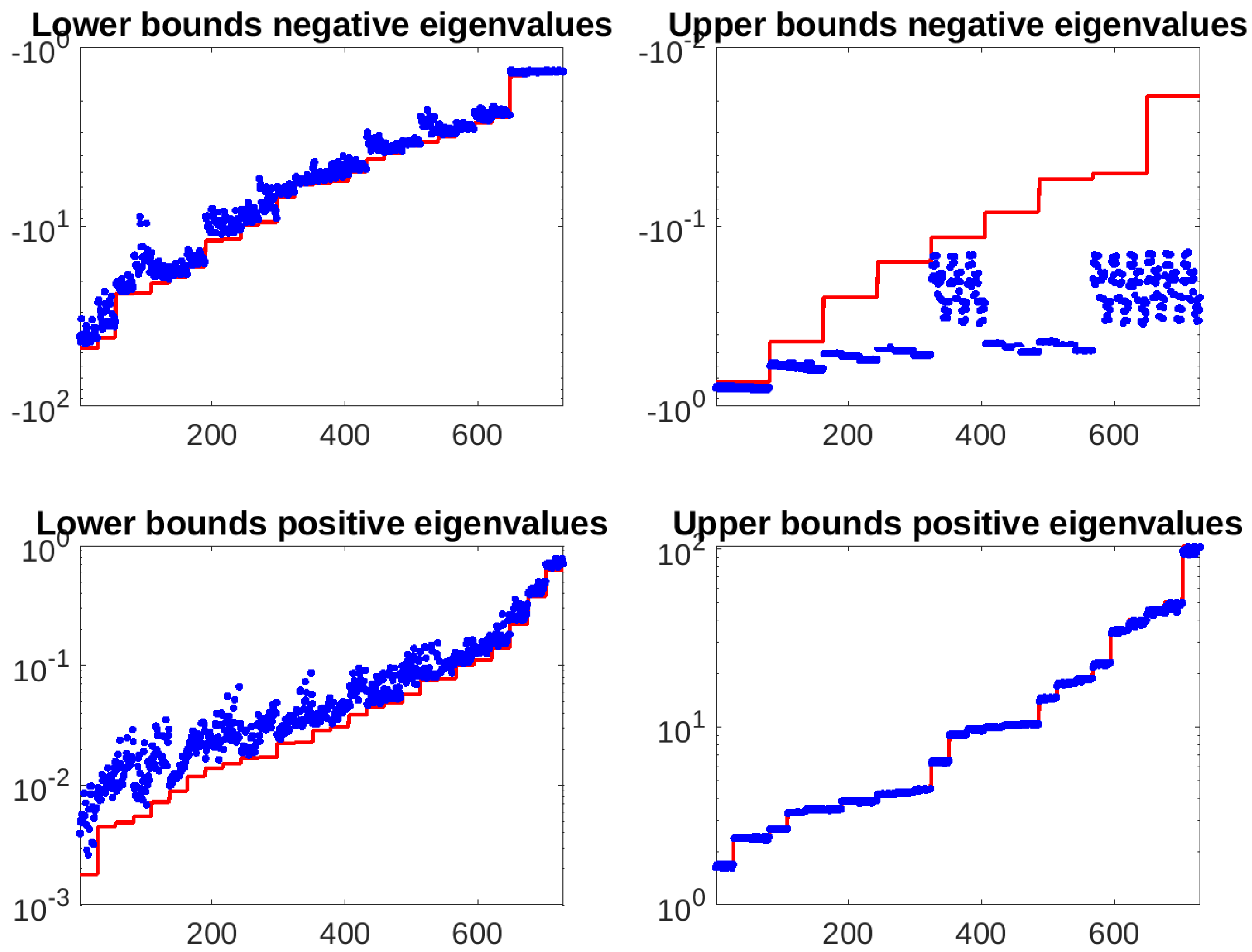
Figure 2.
Multiple saddle-point linear system with . Extremal eigenvalues of the preconditioned matrix (blue dots) and bounds (red line) after 10 runs with each combination of the parameters from Table 1.
Figure 2.
Multiple saddle-point linear system with . Extremal eigenvalues of the preconditioned matrix (blue dots) and bounds (red line) after 10 runs with each combination of the parameters from Table 1.
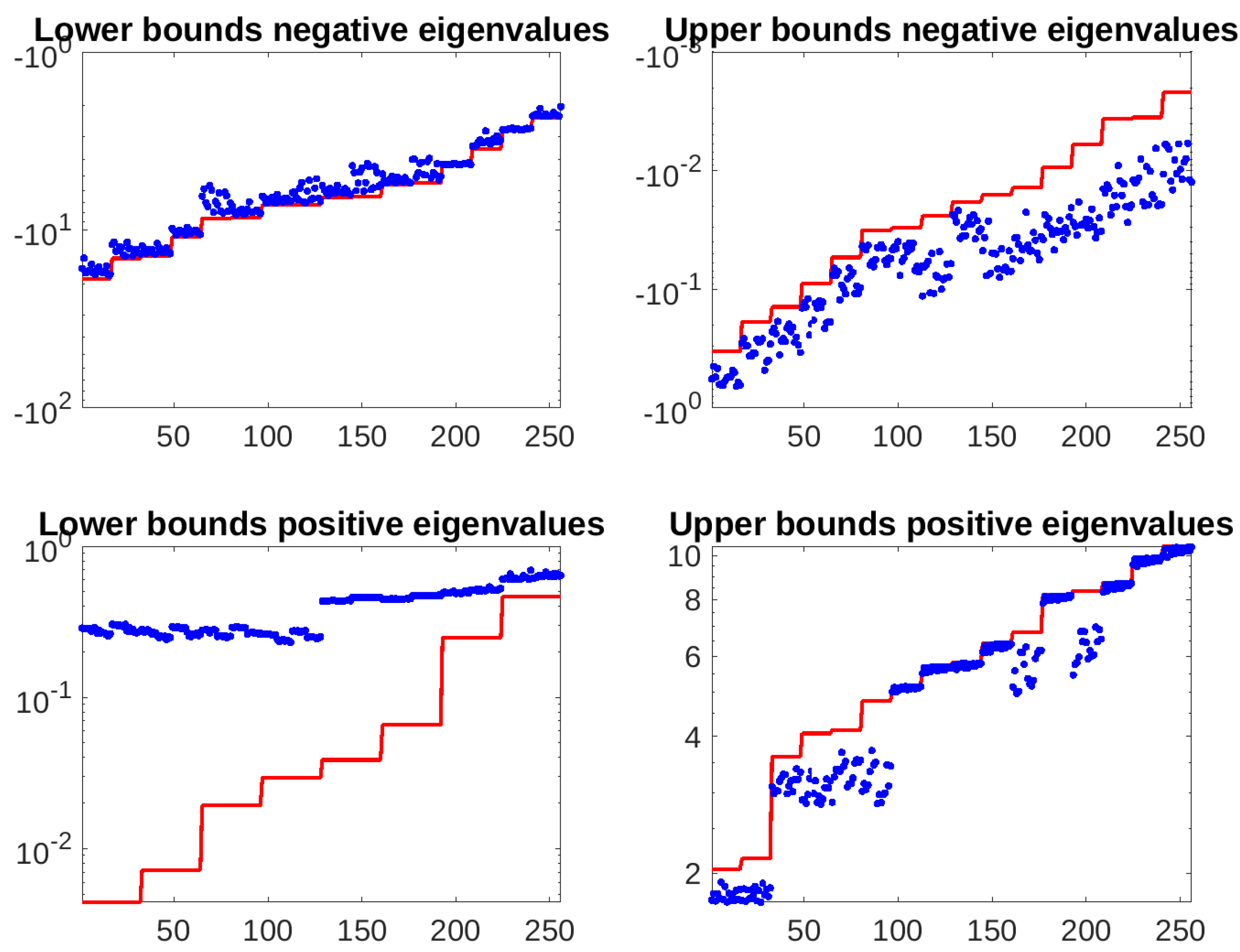
Figure 3.
Multiple saddle-point linear system with . Extremal eigenvalues of the preconditioned matrix (blue dots) and bounds (red line) after 10 runs with each combination of the parameters from Table 1.
Figure 3.
Multiple saddle-point linear system with . Extremal eigenvalues of the preconditioned matrix (blue dots) and bounds (red line) after 10 runs with each combination of the parameters from Table 1.
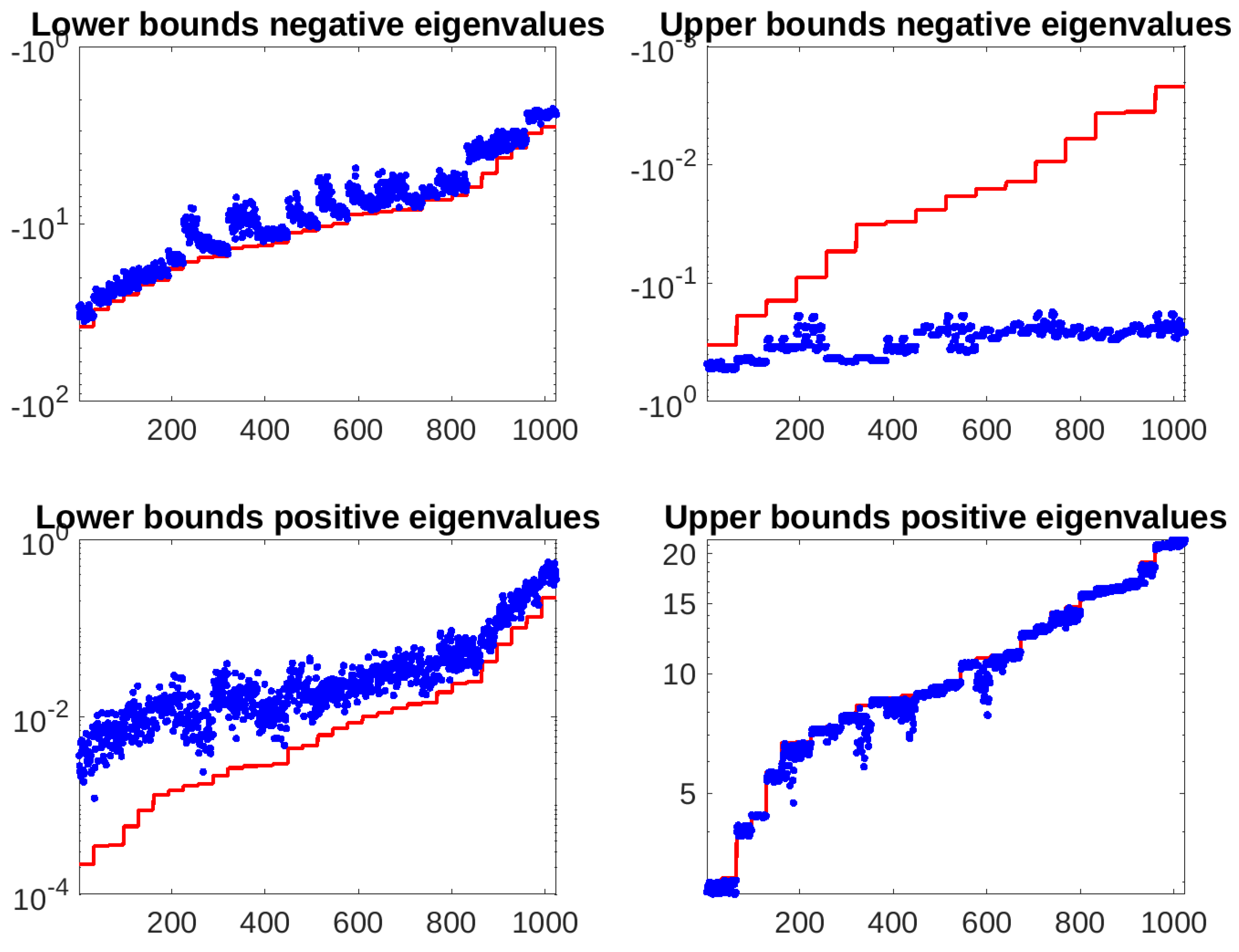
Figure 4.
Iteration numbers of and for all the tests with . The condition number indicator is also displayed.
Figure 4.
Iteration numbers of and for all the tests with . The condition number indicator is also displayed.
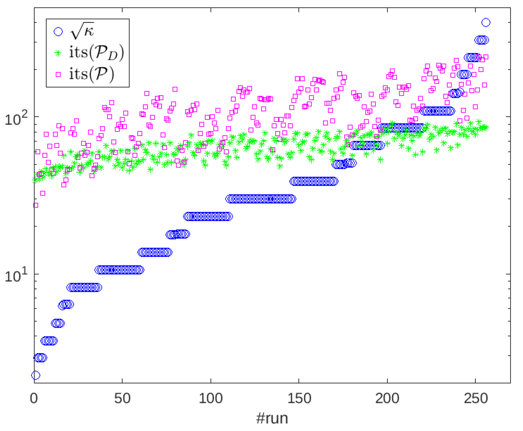
Figure 5.
3D cantilever beam problem. Convergence profiles of MINRES preconditioner with and . Drop tolerance Cholesky parameter: (left), (right).
Figure 5.
3D cantilever beam problem. Convergence profiles of MINRES preconditioner with and . Drop tolerance Cholesky parameter: (left), (right).
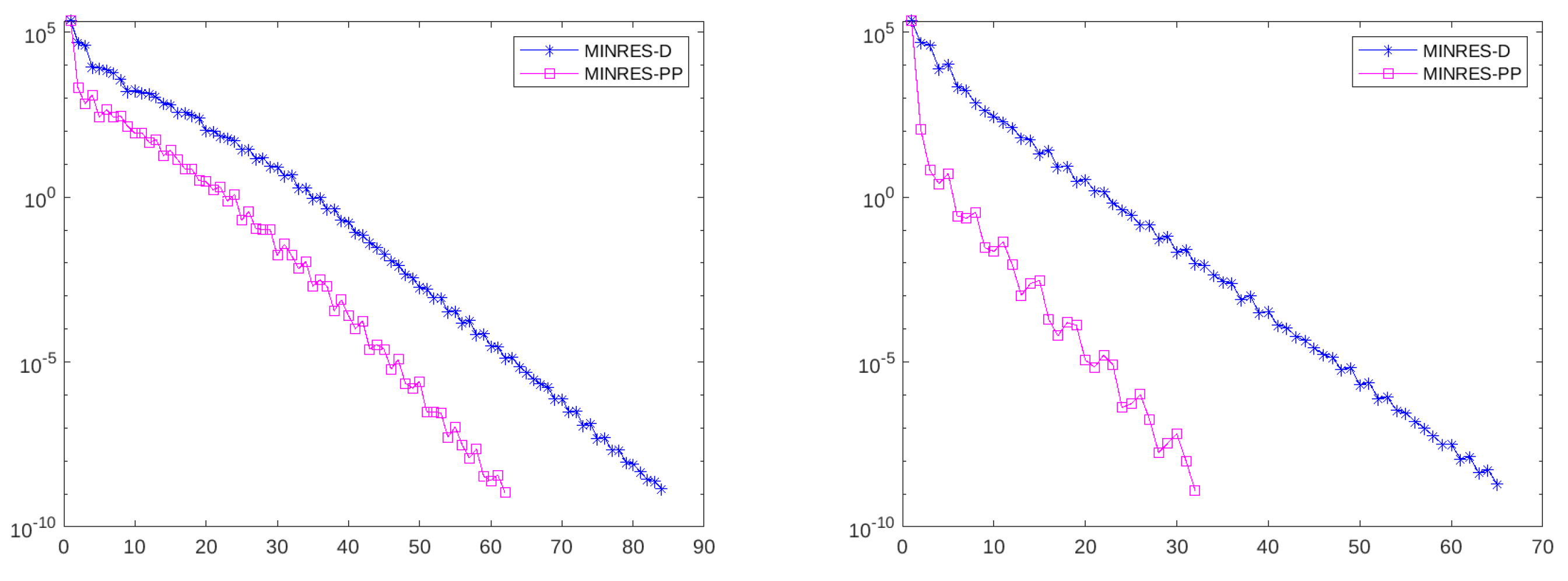

Table 1.
Extremal eigenvalues of the relevant symmetric positive definite matrices used in the verification of the bounds.
Table 1.
Extremal eigenvalues of the relevant symmetric positive definite matrices used in the verification of the bounds.
| 0.1 | 0.3 | 0.9 | 0.1 | 0.8 | ||
| 1.2 | 1.8 | 3 | 1.2 | 2 | ||
| Case | Cases | |||||
Table 2.
3D cantilever beam problem on a unit cube: size and number of nonzeros of the test matrices.
Table 2.
3D cantilever beam problem on a unit cube: size and number of nonzeros of the test matrices.
| nonzeros | |||||
|---|---|---|---|---|---|
| 20 | 27783 | 8000 | 25200 | 60983 | 2.4 |
Table 3.
Extremal values of the indicators for different values of the threshold parameter .
| , | , | , | , | |||||
| , | ||||||||
| , | ||||||||
| , | ||||||||
| , | ||||||||
Table 4.
3D cantilever beam problem on a unit cube: eigenvalue bounds vs real eigenvalues.
| Bounds | -2.6786 | -0.0012 | 0.0424 | 1.2216 | |
| Exact Eigvs | -1.2408 | -0.3192 | 0.0453 | 1.2055 | |
| Bounds | -2.4104 | -0.0012 | 0.2564 | 1.2447 | |
| Exact Eigvs | -1.2408 | -0.3192 | 0.2895 | 1.2252 | |
| Bounds | -1.7001 | -0.0012 | 0.9600 | 1.0119 | |
| Exact Eigvs | -1.2408 | -0.3192 | 0.9600 | 1.0118 | |
| Bounds | -1.6701 | -0.0012 | 0.9976 | 1.0070 | |
| Exact Eigvs | -1.2408 | -0.3190 | 0.9979 | 1.0013 |
Table 5.
Refined eigenvalue bounds vs real eigenvalues.
| Bounds | -2.8268 | -0.2629 | 0.0422 | 1.2274 | |
| Exact Eigvs | -1.2408 | -0.3192 | 0.0453 | 1.2055 | |
| Bounds | -2.4204 | -0.2583 | 0.1809 | 1.2517 | |
| Exact Eigvs | -1.2408 | -0.3192 | 0.2895 | 1.2252 | |
| Bounds | -1.2913 | -0.2951 | 0.9593 | 1.0119 | |
| Exact Eigvs | -1.2408 | -0.3192 | 0.9600 | 1.0118 | |
| Bounds | -1.2434 | -0.3174 | 0.9979 | 1.0029 | |
| Exact Eigvs | -1.2408 | -0.3190 | 0.9979 | 1.0013 |
Table 6.
Number of MINRES iterations for the block diagonal and the PP preconditioner, for different values of the threshold parameter . With we indicate that the exact Cholesky factor of A is used for preconditioning.
Table 6.
Number of MINRES iterations for the block diagonal and the PP preconditioner, for different values of the threshold parameter . With we indicate that the exact Cholesky factor of A is used for preconditioning.
| 0 | |||||
|---|---|---|---|---|---|
| its (diag) | 132 | 83 | 64 | 63 | 63 |
| its (PP) | 99 | 61 | 31 | 23 | 10 |
Disclaimer/Publisher’s Note: The statements, opinions and data contained in all publications are solely those of the individual author(s) and contributor(s) and not of MDPI and/or the editor(s). MDPI and/or the editor(s) disclaim responsibility for any injury to people or property resulting from any ideas, methods, instructions or products referred to in the content. |
© 2026 by the authors. Licensee MDPI, Basel, Switzerland. This article is an open access article distributed under the terms and conditions of the Creative Commons Attribution (CC BY) license (http://creativecommons.org/licenses/by/4.0/).
Copyright: This open access article is published under a Creative Commons CC BY 4.0 license, which permit the free download, distribution, and reuse, provided that the author and preprint are cited in any reuse.


