Submitted:
28 January 2026
Posted:
29 January 2026
You are already at the latest version
Abstract
Climate change is increasingly affecting groundwater resources in the Carpathian Basin, and rising temperatures are expected to increase irrigation demand and pressure on aquifers; the Nyírség region in north-eastern Hungary, a hydraulically coherent recharge–discharge system, provides a suitable setting to investigate these impacts. We analysed multi-decadal groundwater levels from shallow monitoring wells (1970–2022) together with hydroclimate indicators derived from CHIRPS precipitation and ERA5-Land snow and temperature data (1981–2024). Using these inputs, we developed a MODFLOW groundwater flow model for the study area and calibrated it for representative drought and rainy periods, explicitly incorporating permitted withdrawals and estimates of illegal pumping, and applied scenario simulations to assess expected mid-century (2050) climate conditions and human-driven changes, including managed aquifer recharge options. The hydroclimate indicators show strong interannual precipitation variability alongside an overall warming and drying tendency and reduced snow storage. Scenario runs indicate declining shallow groundwater levels, with the largest decreases in higher-elevation areas, while increased pumping primarily intensifies local drawdown near major well fields. Model results suggest that direct subsurface injection is the most effective recharge approach, and water-budget analysis indicates that natural variability can drive subsurface flow changes much larger than those caused by water production, underscoring the need for integrated, long-term measures that include changes in water use.
Keywords:
climate change
; groundwater level decline
; Hungary
; numerical modeling
; managed aquifer recharge (MAR)
; illegal wells
; groundwater governance
; decision support
; digital twin
1. Introduction
Access to water is crucial for human survival and prosperity, forming the basis of well-being and economic development [1,2]. However, there are many signs that climate change is shifting the water cycle towards increased seasonal variability. This results in a more erratic and uncertain supply of both surface water and groundwater [3,4,5,6].
Hydrometeorological trends are changing at a faster rate in the Carpathian Basin, especially in the Great Hungarian Plain, than the global average. The rate of warming is accelerating, and the reconfiguration of major wind systems in the atmosphere is becoming more evident [7]. These changes result in shifts in the spatial and temporal distribution of precipitation, a decline in snowfall and river flow, and variations in the maximum annual water levels of rivers, leading to a general decrease in groundwater levels, particularly in areas of recharge. Declining groundwater levels have led to an increase in both legal and illegal water extraction, which has further exacerbated the situation.
This study analyses the role of natural and anthropogenic impacts in an attempt to predict changes in the groundwater level by 2050. We use numerical simulation to make this prediction and also offer recommendations for mitigating the expected negative impacts. To this end, we focus on a specific sample area: the Nyírség region.
The Nyírség region is located in the north-east of the Hungarian Great Plain. It is the region's highest landscape unit, rising like an island above the surrounding terrain, with an area of 5,100 km² (Figure 1). It has an average altitude of 140 metres above sea level, with the central part exceeding 180 metres and the edges averaging 100–110 metres. The Nyírség is unique in that it is a hydraulically uniform water body, with recharge and discharge areas that belong to it. This makes the region an ideal demonstration area for the combined effects of climate change and human activity on the water balance [8].
Over the past two decades, numerous studies have addressed the spatial analysis of groundwater level changes in the Great Plain [9,10]. One of the main approaches to these analyses is the spatial assessment of changes based on 'groundwater change maps'. In this process, changes in the groundwater level are compared to those in a selected reference period and the difference is depicted on a map using geoinformatics and geostatistical methods. Compared to the 1961–1965 reference period, the effects of rainy and dry periods are most pronounced in the Hátság region, between the Danube and Tisza rivers (the Danube–Tisza Interfluve) and in the Nyírség region. These areas can be considered as recharge areas. The extent of the changes was assessed based on altitude above sea level. In the Danube-Tisza Interfluve region a significant disparity in water scarcity has emerged between areas above and below 120 metres since the mid-1980s. The higher regions have experienced more pronounced scarcity (Figure 2), a phenomenon that emerged a few years later in the Nyírség region (Rakonczai & Fehér, 2019). However, in recent years, the rate of decline in the water level has accelerated, leading to a deterioration in both ecological values and agricultural production. The fact that recharge areas are fed exclusively by precipitation (Tóth, 1963; Tóth, 1999) clearly indicates a change in climatic conditions.
2. Materials and Methods
2.1. Site Description
In terms of structural geology, the eastern and western boundaries of the Nyírség region are well defined, following north-south tectonic lines, while it is bordered by the Tisza River to the north and the Ér Valley to the southeast [11,12,13].
The Nyírség geological formations are characterised by thick layers of Tertiary volcanic rocks, which were deposited on top of a crystalline basement that is not well understood. These volcanic rocks were followed by sediments from the Late Miocene Pannonian Lake, which are between 1000 and 1200 metres thick. During the Pleistocene, the area was uplifted, causing the upper 100–200 metres of the Upper Pannonian formations filling the basin to erode. This was followed by a Quaternary series with an average thickness of 200 m, which was deposited discordantly [14,15]. The thickness of the sediments deposited during the Holocene is less than one metre.
The region was essentially shaped by the surface-forming activity of river water and wind during the Neogene development. The stratigraphic interpretation of the Quaternary fluvial succession was developed in the last decade [16,17,18]. The sedimentation changed from deltaic into alluvial facies associations [11,19,20,21]. The river sediment is thickest along the axis of the Nyírség. All the rivers in the north-eastern part of the Great Plain contributed to the formation of the 120–300-metre-thick layer sequence, the most significant of which were the Tisza and the Szamos [11,19,22]. Some of the river sand turned into aeolian sand, covering large areas to a depth of over 30 metres in places. The gravel, sand and floodplain clay sediments in the deeper basins are arranged in a rhythmic pattern, reflecting the periods of subsidence and the climatic cycles that influence erosion and deposition. The Tertiary hills located between the sub-basins were covered only by drifting sand, falling dust and fine sand or silt from major floods [20,21,23,24] (Figure 3.).
The Pannonian Basin is one of the world's 70 largest aquifer systems [25]. From a hydrodynamic perspective, the Hungarian Great Plain can be divided into two flow systems: a shallower one and a deeper one. The upper system extends from Quaternary to Late Miocene formations, which are highly permeable and porous. This forms an extensive gravitational flow system [22,26]. Meanwhile, a significant overpressure flow system has developed below, primarily due to regional compression and the clay formations of Lake Pannon in the upper sequence [25,27]. This paper focuses on the unconfined, gravitational flow system. The shallow groundwater level follows the contours of the terrain (Figure 4). The Quaternary sediments of the Nyírség region are part of a large, single, leaking aquifer system [22,28], where recharge depends on precipitation infiltrating the surface at higher elevations in the centre. Significant differences exist in the pressure levels of the Upper, Middle and Lower Pleistocene layers [22,28]. In the central areas of Nyírség, for instance, under natural conditions, the difference in piezometric levels of water stored in the Upper and Lower Pleistocene layers was 30–35 metres. This meant that the water level in wells screening the Lower Pleistocene was that much deeper (Figure 5). However, the natural flow system was altered somewhat by the production of water from wells, which began in the mid-19th century and accelerated at the beginning of the 20th century, particularly in the surroundings of the bigger cities [20,22,28].
2.2. Database
2.2.1. Hydrogeological Data
We compiled data on wells from the Water Management Authorities and the National Water Management Directorate, creating a comprehensive database. We checked the data for completeness and corrected the coordinates and data for any wells with errors. In the new database, we have deleted wells with incomplete data. The resulting database contains a total of 3,141 wells. From this large dataset, we selected wells with filters located below 50 m to create a separate database for shallow groundwater wells. Of these, 1,353 have filters located deeper than 50 metres, while 1,788 are shallower than 50 metres. Next, we examined water production. We removed wells with completely inaccurate or missing production data. Between 1978 and 2022, a total of 2,377 wells in the area had time series data. The Water Authorities hold information on the production of illegal wells, which exceeds the total production of legal wells. The methodology subchapter explains how these are taken into account.
Water levels in watercourses and reservoirs (mostly lakes) in the modelling area are documented on a monthly basis. The time period covered by the data series varies greatly, with time series of over 100 years available for major rivers and data for canals available from the 1980s onwards.
2.2.2. Hydroclimate Data Sources
The hydroclimate views implemented in the application are based on a consistent set of datasets accessed through Google Earth Engine and on derived statistics computed in Python. As summarised in Table 1, daily precipitation is obtained from the CHIRPS product, while ERA5-Land provides hourly fields of snow depth, 2 m air temperature and 2 m dewpoint temperature, from which annual means and five-year running averages are calculated. Spatial products, including GeoJSON point samples and interpolated maps, are generated from five-year ERA5-Land composites sampled over the buffered area of interest (AOI). All datasets are accessed through the Google Earth Engine Code Editor or Python API and subsequently processed and visualised in a Python-based CodeStudio environment. The cached AOI-mean daily precipitation time series and the five-year GeoJSON samples constitute reproducible intermediate artefacts that will be distributed alongside the accompanying code repository.
For the illegal-well case study in the Nyerseg region, normalized difference vegetation index (NDVI) and land surface temperature (LST) were derived from Landsat 8 Collection 2 Level-2 Tier 2 imagery acquired between 10 and 26 July 2022 through Google Earth Engine. NDVI was calculated from the near-infrared (Band 5) and red (Band 4) bands, while LST was obtained from thermal Band 10, and both raster products were clipped to the study area. An irrigated-field shapefile was used to delineate agricultural land and to define cropland polygons and their centroids as initial candidate locations for wells. In addition, a point dataset of existing wells, stored in the national Hungarian EOV coordinate system, together with land-cover shapefiles representing forests, water bodies and wetlands, was used to construct buffered exclusion zones. All auxiliary datasets were processed in Python within the same CodeStudio environment as the hydroclimate analysis. Data not directly available through Google Earth Engine, including the irrigated-field shapefile, real-well point layer and land-cover shapefiles, will be released alongside the Earth Engine scripts and Python notebooks in a public repository, subject to the licensing terms of the original data providers.
2.3. Methods
2.3.1. Groundwater Flow Simulation
We used the Processing MODFLOW Pro environment for our hydrodynamic calculations. This software is one of the MODFLOW clones and has extensive calibration references. It supports more MODFLOW packages than other clones and can easily be linked to Surfer, the Windows-based software for map editing and spatial modelling. This environment applies solutions based on the finite difference method for the basic leakage equation, and on the finite difference or characteristic method for the transport equation.
2.3.2. Managed Aquifer Recharge
Managed aquifer recharge (MAR) is the intentional recharge of water into underground aquifers for later recovery or environmental benefit. This involves storing water — such as surface water, stormwater or treated wastewater — in aquifers using infiltration basins, streambeds, recharge wells or riverbank filtration, for example. MAR improves water security, reduces evaporation losses, and improves groundwater quality through natural filtration processes. It is a widely used sustainable water management strategy, particularly in regions where water is scarce [30,31].
2.3.3. Pre-Processing Hydroclimate Data
Daily precipitation data were derived from the CHIRPS global precipitation dataset (Google Earth Engine collection UCSB-CHG/CHIRPS/DAILY). For each day within the study period, precipitation fields were clipped to the analysis geometry and spatially averaged to obtain an AOI-mean daily precipitation time series expressed in millimetres per day; the resulting series was stored as a time-indexed dataframe and cached to ensure consistent reuse across all subsequent analyses and visualizations [32]. Land surface variables were obtained from the ERA5-Land reanalysis as hourly fields accessed through Google Earth Engine, including snow depth, 2 m air temperature and 2 m dewpoint temperature. These hourly variables were clipped to the analysis geometry and aggregated to calendar-year means, with temperature variables converted from Kelvin to degrees Celsius. Unless stated otherwise, all annual statistics were computed for complete calendar years within the user-defined analysis period (data_year_min to data_year_max). A schematic overview of the complete hydrodynamic data workflow and processing steps is provided in Figure 6.
Spatial patterns were examined by aggregating ERA5-Land snow depth and 2 m air temperature into non-overlapping five-year composites. The full analysis period was partitioned into consecutive five-year windows (e.g., 1981–1985 to 2020–2024), within which all hourly ERA5-Land images were averaged to produce mean snow depth and temperature rasters that were subsequently clipped to the buffered analysis geometry. To facilitate data transfer and downstream analysis, each five-year composite was reduced to point samples by generating approximately 4000 pseudo-random locations within the buffered area of interest using a pixelLonLat-based sampling scheme at a nominal spacing of ~10 km; snow depth and temperature values were extracted at these locations, optionally clipped to a shapefile-defined AOI, and exported as GeoJSON files that were bundled for distribution and previewed as scatter maps over the AOI outline. Gridded surfaces were then reconstructed from the GeoJSON samples in Python by interpolating the point values onto a regular grid using radial basis function interpolation, with inverse-distance weighting applied as a fallback when necessary; the resulting grids were masked to the AOI polygon, visualised with standard plotting tools, and differenced between successive five-year windows to quantify the spatial magnitude and direction of change in both snow depth and air temperature.
2.3.4. Temporal Hydroclimate Indicators Calculator Methods
Daily precipitation trends were examined by filtering the cached CHIRPS time series to a user-defined date range and applying a moving-window mean with a selectable length between 1 and 60 days to the AOI-mean precipitation series, producing paired series of raw daily precipitation and smoothed values that facilitate interpretation of individual rainfall events and their temporal persistence. To assess the contribution of different rainfall intensities to annual totals, each daily precipitation value was classified into three intensity categories (<10 mm day⁻¹, 10–30 mm day⁻¹, and >30 mm day⁻¹), and for each calendar year the daily amounts within each category were summed to obtain annual accumulations and their relative contributions to total precipitation. The relationship between heavy rainfall, overall precipitation, and cryospheric and thermal conditions was evaluated by integrating CHIRPS precipitation with ERA5-Land snow depth and 2 m air temperature: annual precipitation totals were calculated by summing daily values, the heavy-rain component was defined as the cumulative precipitation on days exceeding a user-defined threshold (25 mm by default), and annual mean snow depth and air temperature were derived from ERA5-Land and scaled by user-defined factors to allow joint visualization with precipitation on a common chart using separate axes.
Multi-year variability was assessed using trailing five-year moving averages derived from ERA5-Land data. Annual mean snow depth and 2 m air temperature were first calculated for each calendar year and subsequently smoothed using a trailing five-year window, with the initial years incorporating all available preceding data. These smoothed series were displayed together using independent vertical axes to emphasise long-term trends in cryospheric and thermal conditions while preserving interannual variability. Relative humidity was estimated by combining ERA5-Land 2 m air temperature (T) and dewpoint temperature (Td), both converted to degrees Celsius, using a Magnus-type formulation,
after which RH values were constrained to the physical range of 0–100 %, aggregated to annual means, and converted to trailing five-year averages for joint visualization with snow depth and air temperature using separate, colour-matched axes.
2.3.5. Identification of Potential Illegal Wells in the Nyírség Region
The irrigated-field dataset used in this study is based on a polygon provided by the national water authority delineating officially registered irrigated parcels, which was stored and processed as a standard shapefile and served as the basis for all subsequent analyses (Figure 7). The shapefile was first cleaned by merging neighbouring fields using a configurable buffer distance, with before–after geometries examined to verify the integrity of the consolidated field boundaries. The resulting field polygons were then used to generate virtual well locations by placing points randomly around polygon centroids, with parameters controlling the offset range and the number of wells assigned to different field-size classes. These candidate wells were subsequently filtered to remove points located too close to one another or to existing real wells, ensuring appropriate spatial separation and compliance with minimum-distance criteria, and the intermediate results were visually inspected on filtered maps. The final dataset, comprising real wells and the retained virtual wells, was presented as an interactive map that can be exported as an HTML file. To ensure full reproducibility and accessibility, the complete workflow was implemented as an open Streamlit and GitHub project and is publicly available at Abdulhaq. 2025 [33],allowing users to reproduce all cleaning, generation, filtering and visualization steps end-to-end.
2.3.6. Software Environment, Reproducibility and Use of Generative AI
All analyses were conducted for a user-defined area of interest (AOI) using a reproducible workflow that integrates Google Earth Engine (GEE) with Python-based post-processing (Figure 8). The AOI was defined either as a GEE asset (AOI_ASSET_ID) or through an uploaded shapefile; when both were available, the shapefile geometry was used in preference to the asset geometry to define the effective analysis region (analysis_geom). For procedures requiring spatial sampling beyond the nominal AOI, such as the interpolation of gridded surfaces, the analysis geometry was extended by a fixed buffer distance (SAMPLE_BUFFER_METERS) to reduce edge effects. Data acquisition, spatial aggregation and the majority of computationally intensive operations were performed within the GEE environment using both the JavaScript Code Editor and the Earth Engine Python API, whereas subsequent data processing, spatial analysis and visualization were carried out in Python (version 3.x) within a CodeStudio development environment. During development, GitHub Copilot (formerly Codex Copilot) was used to assist with routine coding tasks, with all generated code carefully reviewed and, where necessary, revised by the author.
All data access, computation and visualisation were performed using Google Earth Engine and Python. Time-series aggregation and the majority of raster-based operations were executed within the Google Earth Engine environment through the JavaScript Code Editor and the Earth Engine Python API, whereas subsequent post-processing steps—including cleaning sampled datasets, generating and filtering candidate wells, interpolating five-year spatial products, and producing static and interactive visualisations—were conducted in a Python-based CodeStudio environment using standard scientific and geospatial libraries. The CHIRPS daily precipitation, ERA5-Land reanalysis and Landsat 8 Level-2 datasets employed in this study are publicly available through Google Earth Engine, and all derived products, including AOI-wide hydroclimate time series, five-year GeoJSON samples, interpolated grids and the Categorized_temp.xyz candidate-well dataset, together with the Earth Engine scripts and Python notebooks, will be made available in a public repository upon publication, with no anticipated restrictions on access. Generative artificial intelligence tools were used in a limited and transparent manner, with GitHub Copilot (formerly Codex Copilot) assisting in routine code development and a large language model supporting the refinement of the Materials and Methods text; all AI-assisted outputs were carefully reviewed and revised by the author, who retains full responsibility for the scientific content and interpretation.
3. Results and Discussion
3.1. Groundwater Level Changes
The depth and annual changes of shallow groundwater are also influenced by the flow regime, since the recharge areas are replenished directly by precipitation, with no subsurface inflow [27,34]. In the Nyírség region, areas above 125–130 m are recharge areas, while areas below this level are characterised as flow-through or discharge areas [22,35]. To investigate changes in the groundwater level in the Nyírség region, we analysed more than 50 years' worth of time series data (1970–2022) from 48 shallow groundwater monitoring wells. We plotted the water level time series of the wells against elevation above sea level in 10-metre increments, covering ranges of 100–160 metres. After 2010, it can be observed that there has been no significant decrease in areas below approximately 130 m a.s.l. (Figure 9); the trend in water level decline is similar to that between 1980 and 1995, except for a few wells. In monitoring wells located near large cities, the water level has remained virtually unchanged over the past 50 years, indicating continuous groundwater recharge from leaks in the water supply network. In contrast, in areas above 130 m, most wells experienced a continuous and significant drop in water levels of up to 3 m after 2010. These areas are clear inflow areas that react most quickly to a decrease in the amount of water replenished by infiltration (Figure 10).
From the summer data series consisting of monthly minimum and maximum water levels, we selected June 2010 as the wettest period and September 2022 as the driest, in order to prepare a map of high and low groundwater levels for the entire Nyírség region, based on data from monitoring wells [36,37]. First, we transformed the groundwater levels measured in the wells into a normal distribution using logarithmic transformation [38]. Then, we performed interpolation at the grid nodes using kriging with a composite semivariogram. We then converted these values back to obtain the calculated groundwater level values at the grid points, which we plotted on a map of the Hungarian part of the Nyírség region (Figure 11 and Figure 12). Based on these figures, the groundwater level is at a significant depth of 7 m, even during the wet period. During the dry period, it is deeper than 10 m in the highest part of the Nyírség region [39,40]. At the same time, the groundwater is similarly deep in the north-eastern part of the area despite this being a discharge area along the Tisza River. This is due to the incision of the Tisza valley, which taps into the shallow groundwater [41]. Overall, the difference in water levels between the two studied periods is 1–5 m (Figure 13).
3.1.1. Changes in Water Production Data
To assess the impact of human activity on water resources, we must consider not only shallow groundwater, but also the total water production of the Pleistocene aquifer, including legal and illegal withdrawals. A peculiarity of the Hungarian legal system is that it does not impose penalties for illegally constructed wells. In fact, an amendment to the law in 2023 does not require a permit for the construction of wells shallower than 50 metres for agricultural or domestic use. Consequently, the estimated illegal water production in the Nyírség region exceeds legal production. This estimate is made by the Water Management Authorities using aerial photographs, satellite images and field surveys. Water production has grown steadily over the past 35 years (see Table 2).
We know the exact location and screened depth of all legally drilled wells. According to data from 2022, approximately 10% of legal production comes from the lower Pleistocene (shallow aquifer) layers, 23% from the middle Pleistocene layers and 67% from the most productive lower Pleistocene layers. However, as the exact location and depth of illegal wells are unknown, we developed the method presented in the following chapter.
3.1.1. Location of Illegal Wells, and Production
The workflow starts from a vector shapefile of irrigated field parcels, which defines the candidate agricultural area where unregistered abstraction is most plausible. For the peak growing season, NDVI and Land Surface Temperature (LST) were extracted from the Landsat 8 Level-2 (L2 T2) image collection for 10–26 July 2022. NDVI was computed from the normalized difference of the near-infrared (Band 5) and red (Band 4) bands, while LST was derived from the thermal band (Band 10) and converted to degrees Celsius. Both rasters were clipped to the Nyírség region, then NDVI was used to isolate actively vegetated cropland conditions by selecting pixels in the 0.4-0.6 range (typical of healthy crop cover during the study window). To strengthen interpretation, irrigated parcels were additionally compared against “cold fields” identified from the LST layer, under the assumption that actively irrigated surfaces exhibit locally lower surface temperatures relative to non-irrigated surroundings during hot, dry conditions.
For candidate illegal well delineation, the study area was split into six tiles to support systematic sampling and processing. NDVI and LST values were combined per tile and exported as CSV for cleaning and filtering; only samples meeting the cropland NDVI criterion (0.4–0.6) were retained. Potential well points were then generated around the centroids of irrigated-field polygons, applying spatial logic to reduce unrealistic clustering and edge effects: wells were enforced to be at least 1000 m apart, excluded for parcels smaller than 1000 m² or larger than 100,000 m², and avoided within 1000 m of water bodies and near the study-area boundary. To prevent conflicts with registered infrastructure, candidate wells within 500 m of known real wells were removed using geodesic distance filtering. Remaining candidates were categorized into three temperature classes using LST (Cold/Medium/Warm), with temperatures normalized to 5–16°C (values above 16°C capped) and exported as Categorized_temp.xyz (index 1 = cold/high potential, 2 = medium, 3 = warm/lower potential). A final exclusion step used land-cover shapefiles (forest, water bodies, wetlands) buffered by 100 m to remove candidate wells in restricted zones; coordinates were transformed from Hungarian EOV to WGS84, and the resulting filtered candidates and real wells were visualized in an interactive Folium map and exported to CSV for documentation and further analysis (Figure 14).
3.2. Changes in Climate
Across 1981–2024, total annual precipitation shows pronounced interannual variability, ranging from 461.95 mm (2024) to 896.26 mm (2010) (Figure 15), and declining overall by 220.75 mm from 682.70 mm (1981) to 461.95 mm (2024), although the trajectory is non-monotonic with alternating wet and dry periods. The contribution from heavy rainfall days (>25 mm day⁻¹) is highly episodic and can account for a large share of annual totals, peaking at 213.31 mm (1985) (~one-third of that year’s precipitation), but it is absent in some years (e.g., 1986 and 2024; Figure 15). Notably, the heavy-rain component decreased from 52.69 mm (1981) to 0.00 mm (2024), and its recent disappearance—together with the low 2024 total—suggests a shift toward precipitation dominated by smaller events and/or reduced frequency of threshold-exceeding storms [43].
The snow-depth indicator in Figure 15 (dashed black line; scaled ×250) shows a pronounced long-term decline, indicating reduced snow presence and persistence in the system: snow depth drops from 0.0166 m (1981) to ~0.0019 m (2024) (near-zero), with a maximum of 0.0401 m (1987) and a minimum of ~0.00145 m (2020), and the reduction is most evident during 2010–2024, when values remain consistently low. This loss of snow storage implies a shift in cold-season precipitation toward more rain-dominated inputs and/or weaker accumulation and retention, reducing the snowpack’s role as seasonal water storage, compressing the timing of water release, and potentially shifting runoff earlier while weakening late-season hydrologic buffering [44].
Mean annual air temperature increased from 9.89 °C (1981) to 12.96 °C (2024), corresponding to a net warming of +3.08 °C over the observation period (Figure 15). The warmest conditions occur at the end of the record, while cooler years are concentrated early in the time series (e.g., minimum near the mid-1980s). The co-occurrence of higher temperatures and declining snow depth in the last 15 years supports the interpretation that warming has contributed to a reduced fraction of precipitation retained as snow and to earlier melt or diminished snow persistence [45].
From a water-balance perspective, warming is also expected to increase atmospheric evaporative demand and, consequently, potential evapotranspiration [46]. Higher air temperatures raise the capacity of the atmosphere to hold moisture and often increase vapor pressure deficits, which enhances the “drying power” of the atmosphere [47]. As a result, even when precipitation totals remain within the historical range, a warmer climate can reduce effective water availability by increasing evaporative losses from soils, open water, and vegetation (where water supply permits). Therefore, the warming trend evident in Figure 15 implies that hydrologic stress may intensify not only through changes in precipitation amount and phase (rain vs. snow), but also through enhanced evapotranspiration, which can reduce soil moisture, groundwater recharge potential, and summer baseflow—especially during low-precipitation years such as 2024.
3.2.2. Climate Change Forecast
Climate-change projections for Hungary indicate that the Nyírség region will warm substantially by mid-century under all IPCC-consistent pathways, with scenario-dependent magnitude: an optimistic/low-emission scenario (e.g., SSP1-2.6/RCP2.6) suggests roughly ~+1 °C warming by ~2050, an intermediate scenario (e.g., SSP2-4.5/RCP4.5) about ~+1.5–2 °C, and a pessimistic/high-emission scenario (e.g., SSP5-8.5/RCP8.5) approaching ~+3 °C relative to late-20th-century conditions [48,49] (Figure 16). Note that the historical temperature series used here is based on observed annual-mean weather records, whereas the projections in Figure 16 are climate-model outputs summarized as 30-year daily averages; therefore, differences in baseline level (including the observed record appearing warmer than the modeled projections) reflect both methodological averaging and inherent observation–model differences rather than an inconsistency in the warming trend. Warming is expected to be strongest in summer and autumn, increasing the frequency and intensity of heat extremes and reducing cold conditions (i.e., fewer frost days)—a combination that increases evaporative demand and can intensify agricultural water stress [50]. In parallel, annual precipitation totals are generally projected to change only modestly by ~2050 (often within a few percent), yet the seasonal distribution is expected to shift toward drier summers and slightly wetter winters/autumns, with growing evidence for longer summer dry spells even when annual totals remain near historical levels [50]. Even without large annual changes, precipitation characteristics may become more variable, with a tendency toward more intense downpours and associated runoff/flood risk, particularly outside summer [50].
A robust signal across scenarios is the projected decline in snow depth and snow-cover duration by ~2050, driven primarily by warmer winters that reduce the fraction of precipitation falling and persisting as snow and increase winter rainfall [51]. For a lowland region such as Nyírség, this implies lower maximum snow depths, fewer snow days, and faster melt during cold-season warm spells, weakening the role of snow as seasonal water storage and shifting hydrologic timing toward more rain-dominated winter inputs [51]. In practice, reduced snow storage can diminish seasonal buffering (less delayed release through snowmelt) and, when combined with warming-driven increases in atmospheric demand, can aggravate late-spring and summer water-availability constraints for groundwater-dependent irrigation systems [50,51]. This forecast suggests that infiltration will decrease by 20% by 2050, while evapotranspiration is predicted to rise by 25%.
3.3. Numerical Modeling
3.3.1. Numerical Model Setup
The model covers an area of 129 km north to south and 90.8 km east to west. During modeling, we used a grid size of 200 m. The model was divided vertically into seven layers (Figure 17 and Figure 18):
- Layer 1: mostly Holocene unconfined aquifers.
- Layer 2: Upper Pleistocene fine sandy aquifers
- Layer 3: clayey semi-aquitard with sand interlayers
- Layer 4: middle Pleistocene sandy aquifer;
- Layer 5: clayey sequitard mi-awith sand interlayers.
- Layer 6: Lower Pleistocene sandy and coarse sandy aquifer, or 'waterworks layer'.
- Layer 7: Layer simulating the effect of wells under Pleistocene formations to determine lower boundary conditions (mostly Late Miocene sediments from Dunántúli Group).
When determining the hydrogeological characteristics of the model layers, we considered the hydrogeological logs of the wells, as well as the outcomes of regional sequence stratigraphic studies [16,17,18] (Table 3). Potentiometric levels were determined using data from network monitoring (Figure 17).
The infiltration values used are proportional to the amount of precipitation that recharges the subsurface formations. Both the unsaturated zone and groundwater evapotranspiration, as well as vegetation water uptake, draw from these formations. This means that the infiltration value does not include surface runoff. In this case, infiltration is primarily dependent on topography, with values ranging from 120 to 250 mm per year (Figure 19). These values were slightly modified during calibration. In the base state of the model, the maximum evapotranspiration value at the surface was 708 mm per year, decreasing linearly to a depth of 5.8 metres, at which point it reached 0. Rivers and major canals in the study area were incorporated into the model using hydrological longitudinal profiles.
The most important consideration when selecting boundary conditions was to ensure that their effects influenced the calculation results as little as possible while maintaining stable water flow. Taking into account the natural boundaries of the groundwater level at the edges of the model — i.e. rivers — we only applied boundary conditions where absolutely necessary, to minimise disruption to water flow. However, for deeper layers, we had to specify a soft boundary condition (GHB), as the water flow at the boundaries is mostly horizontal. This boundary condition type also allows pressure level changes in the boundary cells if necessary, adjusting the water balance of the cell in proportion to the resulting depression. In the case of the lowest, 7th model layer, which represents the upper part of the Dunántúli Group (Late Miocene), it also ensures the lower openness of the model as a GHB boundary surface. Its value was set during calibration.
3.3.2. Numerical Model Calibration
The model was calibrated using data from two selected years: the wet year of 2010 and the dry year of 2022, for which 120 monitoring well data were used. During calibration, we adjusted the values for the hydraulic conductivity, infiltration from precipitation and evapotranspiration, as well as the extent of illegal water withdrawal. Furthermore, as the water level in the wells near the Tisza River in the eastern part of the model was higher than the measured value during the simulation, we increased the conductance of the Tisza riverbed sediment tenfold (i.e. we increased the riverbed hydraulic conductivity). This is also likely due to the presumed incision of the riverbed.
Total water production during the dry season rose from 110 million m³ per year to approximately 124 million m³ due to the increase in illegal water withdrawals. At the same time, a significant difference in production and infiltration was observed between the two periods. Analysis of production data revealed that total water production decreased by around 15% during the wet period compared to the dry period, with varying degrees of reduction observed between layers. Meanwhile, infiltration increased by around 30%. The rise in the water level in rivers and canals varied between 1 and 3 metres.
Based on the five-step calibration, the variance calculated for the dry period was 2.33, whereas for the wet period it was 3.97 (Figure 20 and Figure 21). During calibration, the difference between the calculated and measured water levels remained within 0.5 m for most wells, with only a few exceeding 2 m. It is unrealistic to expect to achieve significantly lower values, given that the model uses average values for areas measuring 200 x 200 metres.
3.3.3. Numerical Model Results and Forecast for 2050
Using the calibrated model, we ran simulations to work out the water levels for 2022, a period that is similar to the current situation (Figure 22). According to these results, the water level in shallow aquifers decreased by an average of 0.5–1.5 metres compared to the 2010 period. The greatest decrease occurred in river valleys and elevated areas (Figure 23).
Looking ahead, based on the climate scenarios presented, we estimate a 20% decrease in infiltration by 2050. Meanwhile, evapotranspiration is expected to increase by 25% compared to the current dry season. To compensate for this, we anticipate that water production will increase by around 20%. We have created a separate model to illustrate and compare the effects of climate change and increased water production.
According to the model that simulates extreme dry climatic periods, a decrease in the level of shallow groundwater of more than 0.25 metres is expected in most of the studied area. However, in regions with significantly higher elevations, this value may reach up to 1.25 metres (see Figure 24).
In the next model variant, we increased the production at all wells by 20% without changing their locations. In this case, the largest part of the model area experiences a decrease in the shallow groundwater level of less than 0.1 m, with the greatest reductions occurring at significant water extraction sites located in the recharge area. This is particularly true of Debrecen, the largest settlement in the area. Significant water production takes place there, accounting for around 10% of the total water extraction in the Nyírség region. Here, the rate of water level decline due to water production is close to the rate of water level decline due to climatic effects. (Figure 25).
Analysis of water budget data shows that, although maximum evapotranspiration is 25% higher during periods of extreme drought, the lower infiltration rate and decrease in groundwater levels mean the total amount is still lower. Under dry climatic conditions (in 2022), it is 1,933 million m³ per day; under extremely dry conditions (in 2050), it is 1,521 million m³ per day. This has led to a greater degree of atmospheric drought, i.e. a significant decrease in humidity. If extremely dry conditions persist, the levels of the middle and lower Pleistocene aquifers (model layers 4 and 6) will decrease slightly due to leakage in the groundwater flow system (Figure 26 and Figure 27).
3.4. Proposed Actions Using a Numerical Model
By determining the amount of water lost due to the drop in shallow groundwater levels caused by extreme drought, we can estimate the scale of the artificial water replenishment task. First, we used the Surfer program to determine the volume of water that had decreased in the shallow aquifer. Between 2010 and 2022 this equated to 5.21 km³, which, when the area of Nyírség is taken into account, represents an average decrease in the water level of 102 cm. Assuming 20% porosity, this volume equates to a water shortage of 1042 million m³. According to our forecast, an additional 2.55 km³ of water will have been depleted by 2050. Assuming 20% porosity, this equates to a water shortage of 510 million cubic metres, corresponding to an average decrease in water levels in the shallow aquifer of 50 cm. In other words, looking ahead to 2050, the impact of climate change since 2010 will result in a water shortage equivalent to more than ten times the annual water production. This cannot be artificially replenished, so the impact can only be reduced. MAR technology has long-term positive effects on groundwater resources, providing economic, social and environmental benefits [52]. In this study, we will simulate two of these effects: infiltration from surface reservoirs and water injection through wells.
3.4.1. MAR - Replenishment of Rivers and Lakes
The water management authorities have developed plans for possible water replenishment. To simulate one of these proposals, we selected a 15x13 km area in the north-eastern part of the model and rotated it by 18 degrees. This ensured that the western and eastern edges were perpendicular to both the surface slope and the equipotential lines. (Figure 28). To better observe changes in the water level, we used a vertical resolution of 10 metres and a horizontal resolution of 5 metres. We then examined the effect of changes in the surface water drainage system (2 lakes and 2 channels) on shallow groundwater levels in the area. Studying the longitudinal profiles of the channels, we modelled a 1-metre rise for the channels and a 1.5-metre rise for the lakes. We did not allocate the necessary structures and assumed that water would be transported to the highest areas via pipelines, then released at a planned flow rate of 3–5 m³/s. We determined the hydraulic conductivity of the colmated lake sediments to be 0.001 m/d, with a thickness of 0.5 m. For the 2 m-wide channels, these values are 0.0024 m/d and 0.33 m, respectively. The channels were modelled using the Stream package.
The results are shown in Figure 29. In the bands parallel to the channels, the water level rises by a few decimetres, whereas in the lakes it rises by 1 metre. The edge of the impact area was defined as a rise of 5 cm, which, in constant modelling, is 180–300 metres from the channel. In the case of lakes, this value is 800–1,200 metres. Lower values occur in northern lakes, while higher values occur in southern lakes.
To achieve a more realistic result, we performed transient modelling over a period of five years. Each year, water replenishment took place for four months using the values specified in the permanent model. For the remaining eight months, there was no water replenishment, and evaporation increased by 25%. As expected, the shallow groundwater level gradually rose at the end of the replenishment periods (Figure 30), as confirmed by the time series data of virtual observation wells located 1, 25, 75, 175 and 375 metres from the lakes (Figure 31). Although the rise in shallow groundwater levels reached one metre in the immediate vicinity of the lakes, its influence only extended 150–400 metres by the end of the fifth replenishment period (Figure). In contrast, the rise in water levels in the canals was barely detectable. By the end of the dry period in the fifth year, the rise in water levels in the vicinity of the lakes was 0.2–0.3 metres, shifting in a west-northwest direction corresponding to the direction of groundwater flow (Figure 30d).
3.4.2. MAR - Subsurface Water Recharge
A special method of recharging the aquifer involves using wells to inject water through drainage pipes [31,53]. This allows larger quantities of water to be pumped in without causing a significant rise in the water level at a particular location. The amount of water infiltrating and evaporating can be determined using the water budget based on the infiltration through lakes method presented in the previous subsection. Using the drainage injection method to inject this total amount of water directly below the surface can increase the amount of water feeding the groundwater by around 30%.
We modelled this case by injecting the amount of water infiltrating and evaporating from the northern lake, as calculated in the previous model, into a drainage system located near the lake and used for infiltration in the previous scenario, rather than into the lake itself. The drain was set to a length of 3 x 700 metres to ensure that the maximum rise in water level would not exceed 5 metres. In this case, the effective range of artificial water recharge, which raises the water level by at least 5 cm, increased from 800–100 metres to 1,000–1,250 metres (Figure 32).
3.4.3. Changing the Agricultural Cultivation System
To improve groundwater decision making in the Nyírség region, we recommend moving toward a data-driven groundwater management system that integrates monitoring and operational information into a single, continuously updated workflow. The key rationale is that the main stressors—possible overextraction, limited/uneven monitoring coverage, and climate-driven variability in recharge and demand—cannot be evaluated reliably when data remain fragmented across institutions, formats, and time scales. As a practical first step, the existing digital platform developed for the General Directorate of Water Management of Hungary (which already compiles historical well information and annual/monthly abstraction records for the Nyírség area) should be strengthened as a shared data infrastructure (standardized identifiers, quality control, consistent time steps, and spatial referencing). We suggest that this infrastructure be designed explicitly to support an updatable groundwater “digital twin”—a model framework that is periodically recalibrated with new groundwater levels, pumping volumes, and relevant hydroclimatic drivers—so that resource status can be tracked in near-real time and management actions can be evaluated against measurable indicators (e.g., groundwater-level thresholds and trend-based early warnings).
Building on this foundation, we further recommend that the system be used not only for monitoring but also to optimize the agricultural cultivation system in terms of water efficiency by translating hydrogeologic constraints into extraction limits and operational guidance. Concretely, the digital twin can be used to define adaptive caps (monthly/seasonal/annual) on allowable abstraction at the well or management-unit scale, triggered by groundwater-level thresholds and expected seasonal recharge, and then link these limits directly to irrigation operations. In parallel, the platform should monitor agricultural variables that strongly control water demand—especially crop type, cultivated area, and cropping calendar—and generate recommendations that improve water efficiency (e.g., irrigation scheduling, application-efficiency improvements, and allocation rules) while remaining within the extraction caps. Importantly, crop selection should be treated as part of the decision-support loop: the system can support recommendations to avoid or restrict high water-demand crops in stressed areas or dry years and instead encourage more water-efficient or drought-tolerant crop types/varieties, thereby aligning permitted groundwater withdrawals with crop water requirements and reducing the risk that agricultural planning drives unsustainable pumping.
4. Conclusions
This study shows that the Nyírség is an effective 'early warning' landscape for climate-driven groundwater stress in the Hungarian Great Plain because it is a hydraulically coherent recharge–discharge system. Long-term monitoring records indicate a clear intensification of shallow groundwater decline after 2010 in higher-elevation recharge areas (roughly above 125–130 m a.s.l.), while lower areas show weaker or more buffered changes. However, significant water level decreases also occurred in river valleys located on the edge of the study area. Hydroclimate indicators derived from CHIRPS and ERA5-Land reveal strong interannual variability in precipitation, as well as a consistent warming trend and a marked decline in snow storage. These factors reduce effective recharge and increase evaporative demand.
By integrating these observations with a calibrated numerical groundwater flow model, we demonstrated that the mid-century risk of groundwater depletion in the Nyírség region is primarily driven by reduced infiltration and increased evapotranspiration. Scenario simulations for 2050 suggest a further widespread decline in shallow groundwater levels, with the greatest reductions occurring in the elevated recharge zone. Increased withdrawals amplify groundwater drawdown, creating local hotspots near major pumping centres. While artificial recharge measures can facilitate local recovery near lakes, the simulated transient influence radius remains limited. Model data indicate that direct underground injection of water into the aquifer is the most effective method of managed aquifer recharge. However, the results imply that MAR alone cannot offset basin-scale deficits; while human activity can mitigate or amplify negative changes, it cannot alter their direction. Overall, the outcomes emphasise the necessity of combining strategies, such as targeted recharge where feasible, enhanced monitoring and management of withdrawals (including unregistered abstraction) and demand-side measures in agriculture. These strategies must be underpinned by integrated data and modelling processes.
Although the Nyírség region is only a small part of the Carpathian Basin, it is extremely important to study it. This is because the effects observed here can be used to predict those that will be seen in the lowland areas, and the region provides an ideal testing ground for finding solutions to the problem.
Author Contributions
Conceptualization, J.S., H.A.A., R.H., É.S. and L.L.; methodology, J.S., H.A.A. and R.H.; software, J.S., H.A.A. and E.T.; validation, J.S. and E.T.; formal analysis, J.S. and H.A.A.; investigation, J.S. and H.A.A.; resources, J.S., H.A.A. and R.H.; data curation, J.S., H.A.A., R.H. and T.G.; writing—original draft preparation, J.S., H.A.A. and R.H.; writing—review and editing, J.S., H.A.A. and R.H.; visualization, J.S., H.A.A., T.G. and E.T.; supervision, J.S. and H.A.A.; project administration, R.H., É.S. and L.L.; funding acquisition, R.H.
Funding
The research presented in this article was carried out within the framework of the Széchenyi Plan Plus Programme, with the support of the RRF 2.3.1-21-2022-00008 project.
Data Availability Statement
The data supporting the reported results are publicly available on Zenodo and are cited in the manuscript where relevant (including the authors’ own Zenodo deposits).
Acknowledgments
The authors gratefully acknowledge the support of the General Directorate of Water Management (Országos Vízügyi Főigazgatóság – OVF), the Upper-Tisza Regional Water Directorate (Felső-Tisza-vidéki Vízügyi Igazgatóság – FETIVIZIG), and the Trans-Tisza Region Water Directorate (Tiszántúli Vízügyi Igazgatóság – TIVIZIG), as well as their teams, for assistance that supported this study. We also acknowledge Google Earth Engine for providing the computing platform used in this research.
Conflicts of Interest
The authors declare no conflicts of interest. The funders had no role in the design of the study; in the collection, analyses, or interpretation of data; in the writing of the manuscript; or in the decision to publish the results.
References
- Ecosystem-Based Water Security and the Sustainable Development Goals (SDGs) Available online: https://www.conservation.org/research/ecosystem-based-water-security-and-the-sustainable-development-goals-(sdgs) (accessed on 17 December 2025).
- Mishra, B.K.; Kumar, P.; Saraswat, C.; Chakraborty, S.; Gautam, A. Water Security in a Changing Environment: Concept, Challenges and Solutions. Water 2021, 13, 490. [CrossRef]
- Chapter 8: Water Cycle Changes | Climate Change 2021: The Physical Science Basis Available online: https://www.ipcc.ch/report/ar6/wg1/chapter/chapter-8/ (accessed on 17 December 2025).
- Intergovernmental Panel On Climate Change (Ipcc) Climate Change 2021 – The Physical Science Basis: Working Group I Contribution to the Sixth Assessment Report of the Intergovernmental Panel on Climate Change; 1st ed.; Cambridge University Press, 2023; ISBN 978-1-009-15789-6.
- Hidrológiai Közlöny, 2018 (98. Évfolyam) | Könyvtár | Hungaricana Available online: https://library.hungaricana.hu/hu/view/HidrologiaiKozlony_2018/?pg=260&layout=s (accessed on 17 December 2025).
- Bartholy, J. REGIONAL CLIMATE CHANGE EX PECTED IN HUNGARY FOR 2071-2100. Appl. Ecol. Environ. Res. 2007, 5, 1–17. [CrossRef]
- Jánosi, I.M.; Bíró, T.; Lakatos, B.O.; Gallas, J.A.C.; Szöllosi-Nagy, A. Changing Water Cycle under a Warming Climate: Tendencies in the Carpathian Basin. Climate 2023, 11, 118. [CrossRef]
- Szanyi, J. The Influence of Lower-Boundary Condition on the Groundwater Flow System. Acta Geol. Hung. 2005, 47, 93–103. [CrossRef]
- Rakonczai J.; Fehér Z.Zs. A talajvízkészlet változásának értékelése hazánkban; Viziterv Environ Kft, 2019;
- Rakonczai J.; Fehér Z.Zs. A klímaváltozás szerepe az Alföld talajvízkészleteinek időbeli változásaiban. Hidrol. Közlöny 2015, 95, 1–15.
- Püspöki, Z.; Demeter, G.; Tóth-Makk, Á.; Kozák, M.; Dávid, Á.; Virág, M.; Kovács-Pálffy, P.; Kónya, P.; Gyuricza, Gy.; Kiss, J.; et al. Tectonically Controlled Quaternary Intracontinental Fluvial Sequence Development in the Nyírség–Pannonian Basin, Hungary. Sediment. Geol. 2013, 283, 34–56. [CrossRef]
- Csontos, L.; Nagymarosy, A.; Horváth, F.; Kovác, M. Tertiary Evolution of the Intra-Carpathian Area: A Model. Tectonophysics 1992, 208, 221–241. [CrossRef]
- Marton L.; Szanyi J. A talajvíztükör helyzete és a rétegvíz termelés kapcsolata Debrecen térségében. Hidrol. Közlöny 2000.
- Horváth, F.; Tari, G. IBS Pannonian Basin Project: A Review of the Main Results and Their Bearings on Hydrocarbon Exploration. In The Mediterranean Basins: Tertiary Extension within the Alpine Orogen; Durand, B., Jolivet, L., Horváth, F., Séranne, M., Eds.; Geological Society Special Publications; The Geological Society: London, 1999; Vol. 156, pp. 195–213.
- Horváth, F.; Cloetingh, S. Stress Induced Late-Stage Subsidence Anomalies in the Pannonian Basin. In Dynamics of Extensional Basins and Inversion Tectonics; Cloetingh, S., Ben Avraham, Z., Sassi, W., Horváth, F., Eds.; 1996; Vol. 266, pp. 287–300.
- Püspöki, Z.; Markos, G.; Fancsik, T.; Bereczki, L.; Kiss, L.F.; Thamó-Bozsó, E.; Krassay, Z.; Kovács, P.; McIntosh, R.W.; Vári, Z.; et al. A Quasi-Continuous Long-Term (5 Ma) Mid-European Mountain Permafrost Record Based on Fluvial Magnetic Susceptibility and Its Contribution to the Explanation of Plio-Pleistocene Glaciations. Boreas 2024. [CrossRef]
- Püspöki, Z.; Kovács, I.J.; Fancsik, T.; Nádor, A.; Thamó-Bozsó, E.; Tóth-Makk, Á.; Udvardi, B.; Kónya, P.; Füri, J.; Bendő, Z.; et al. Magnetic Susceptibility as a Possible Correlation Tool in Quaternary Alluvial Stratigraphy. Boreas 2016, 45, 861–875. [CrossRef]
- Püspöki, Z.; Fogarassy-Pummer, T.; Thamó-Bozsó, E.; Falus, G.; Cserkész-Nagy, Á.; Szappanos, B.; Márton, E.; Lantos, Z.; Szabó, S.; Stercel, F.; et al. High-resolution Stratigraphy of Quaternary Fluvial Deposits in the Makó Trough and the Danube-Tisza Interfluve, Hungary, Based on Magnetic Susceptibility Data. Boreas 2021, 50, 205–223. [CrossRef]
- Borsy Z. A Nyírség természeti földrajza; Akadémiai Kiadó: Budapest, 1961;
- Flores, Y.G.; Eid, M.H.; Szűcs, P.; Szőcs, T.; Fancsik, T.; Szanyi, J.; Kovács, B.; Markos, G.; Újlaki, P.; Tóth, P.; et al. Integration of Geological, Geochemical Modelling and Hydrodynamic Condition for Understanding the Geometry and Flow Pattern of the Aquifer System, Southern Nyírség–Hajdúság, Hungary. Water 2023, 15, 2888. [CrossRef]
- Nádor, A.; Sztanó, O. Lateral and Vertical Variability of Channel Belt Stacking Density as a Function of Subsidence and Sediment Supply: Field Evidence from the Intramountaine Körös Basin, Hungary. In From River to Rock Record; SEPM Special Publications; 2010; Vol. 99.
- Marton L. A környezeti izotópok felhasználása a Nyírség negyedkori mélységbeli vizeinek kutatásában. Kandidátusi értekezés, 1981.
- Kőrössy L. A zalai-medencei k?olaj- és földgázkutatás földtani eredményei. Ált. Földt. Szle. 1988, 3–162.
- Rónai A. Az Alföld tájai. In Geologica Hungarica; Rónai A., Ed.; Series 21; Műszaki Könyvkiadó: Budapest, 1985; pp. 258–407.
- Almási, L.; Szanyi, J. Hydrogeology of the Pannonian Basin. In The Groundwater Project and eBooks – Important Aquifer Systems Around The World; 2024.
- Erdélyi, M. A Magyar Medence hidrodinamikája =: Hydrodynamics of the Hungarian Basin; VITUKI: Budapest, 1979; ISBN 978-963-511-068-1.
- Tóth, J.; Almási, I. Interpretation of Observed Fluid Potential Patterns in a Deep Sedimentary Basin under Tectonic Compression: Hungarian Great Plain, Pannonian Basin. Geofluids 2001, 1, 11–36. [CrossRef]
- Szanyi J. Felszín alatti víztermelés környezeti hatásai a Dél-Nyírség példáján. PhD disszertáció, Szegedi Tudományegyetem (SZTE).
- Tóth, G.; Kun, É.; Kerékgyártó, T. Szabolcs-Szatmár-Bereg megye mintaterületére készült vízkészletgazdálkodási modell; Hungarian water management authority: Hungary, 2021;
- Managed Aquifer Recharge: Overview and Governance; Dillon, P., Alley, W., Zheng, Y., Vanderzalm, J., Eds.; IAH Special Publication; 2022; ISBN 978-1-3999-2814-4.
- Sufyan, M.; Martelli, G.; Teatini, P.; Cherubini, C.; Goi, D. Managed Aquifer Recharge for Sustainable Groundwater Management: New Developments, Challenges, and Future Prospects. Water 2024, 16, 3216. [CrossRef]
- Abdulhaq, H. Earth Engine Hydroclimate Dashboard (Streamlit) 2025.
- Abdulhaq, H. Geoscience & Data Visualization Python Toolkit (Streamlit, Mapping, Interpolation, and Stats) 2025.
- Tóth, J. A Theoretical Analysis of Groundwater Flow in Small Drainage Basins. J. Geophys. Res. 1896-1977 1963, 68, 4795–4812. [CrossRef]
- Felszín Alatti Víztermelés Környezeti Hatásai a Dél-Nyírség Példáján - SZTE Repository of Dissertations Available online: https://doktori.bibl.u-szeged.hu/id/eprint/335/ (accessed on 13 January 2026).
- djrust26 Aszály a Nyírségben – Már az év eleje is csapadékmentesen indult 2022-ben Available online: https://www.nyiregyhaza.hu/post/aszaly-a-nyirsegben-mar-az-ev-eleje-is-csapadekmentesen-indult-2022-ben-2022-05-25 (accessed on 30 December 2025).
- MNO A talajvíz szintje megdöntötte az 1936-os rekordot is + Képriport Available online: https://magyarnemzet.hu/archivum-archivum/2010/12/a-talajviz-szintje-megdontotte-az-1936-os-rekordot-is-kepriport (accessed on 30 December 2025).
- FENG, C.; WANG, H.; LU, N.; CHEN, T.; HE, H.; LU, Y.; TU, X.M. Log-Transformation and Its Implications for Data Analysis. Shanghai Arch. Psychiatry 2014, 26, 105–109. [CrossRef]
- Simon, S.; Déri-Takács, J.; Szijártó, M.; Szél, L.; Mádl-Szőnyi, J. Correction: Simon et al. Wetland Management in Recharge Regions of Regional Groundwater Flow Systems with Water Shortage, Nyírség Region, Hungary. Water 2023, 15, 3589. Water 2024, 16, 1609. [CrossRef]
- Belügyminisztérium Magyarország 2021. Évi Vízgyűjtő-Gazdálkodási Terve: „A Duna-Vízgyűjtő Magyarországi Része Vízgyűjtő-Gazdálkodási Terv – 2021” Dokumentumának Összefoglaló Rövidített Változata; Belügyminisztérium, 2022;
- Czomba, P.; Vass, R.; Túri, Z. Statistical Analysis of the Hydrological and Hydrometeorological Characteristics of the Upper Tisza Basin. J. Environ. Geogr. 2023, 16, 133–139. [CrossRef]
- Völgyesi, I. A Nyírségi régió felszín alatti vízháztartása, kitermelhető vízkészlete 2004.
- Kovács, A.; Jakab, A. Modelling the Impacts of Climate Change on Shallow Groundwater Conditions in Hungary. Water 2021, 13, 668. [CrossRef]
- Varlas, G.; Papadaki, C.; Stefanidis, K.; Mentzafou, A.; Pechlivanidis, I.; Papadopoulos, A.; Dimitriou, E. Increasing Trends in Discharge Maxima of a Mediterranean River during Early Autumn. Water 2023, 15, 1022. [CrossRef]
- Pérez-Palazón, M.J.; Pimentel, R.; Polo, M.J. Climate Trends Impact on the Snowfall Regime in Mediterranean Mountain Areas: Future Scenario Assessment in Sierra Nevada (Spain). Water 2018, 10, 720. [CrossRef]
- Water Balance Trends along Climatic Variations in the Mediterranean Basin over the Past Decades Available online: https://www.mdpi.com/2073-4441/15/10/1889 (accessed on 6 January 2026).
- Assessing Climate Change Impacts on Spring Discharge in Data-Sparse Environments Using a Combined Statistical–Analytical Method: An Example from the Aggtelek Karst Area, Hungary Available online: https://www.mdpi.com/2073-4441/17/17/2507 (accessed on 6 January 2026).
- Bartholy, J.; Pongrácz, R.; Pieczka, I. How the Climate Will Change in This Century? Hung. Geogr. Bull. 2014, 63, 55–67. [CrossRef]
- ClimateChangePost Climate Change Available online: https://www.climatechangepost.com/countries/hungary/climate-change/ (accessed on 16 January 2026).
- Hungary Climate Resilience Policy Indicator – Analysis Available online: https://www.iea.org/articles/hungary-climate-resilience-policy-indicator (accessed on 16 January 2026).
- Kis, A.; Pongrácz, R. Future Changes of Snow-Related Variables in Different European Regions. Hung. Geogr. Bull. 2023, 72, 3–22. [CrossRef]
- Managing Aquifer Recharge: A Showcase for Resilience and Sustainability; Zheng, Y., Ross, A., Villholth, K.G., Dillon, P., Eds.; UNESCO: Paris, 2021;
- Nightingale, H.I.; Ayars, J.E.; McCormick, R.L.; Cehrs, D.C. Leaky Acres Recharge Facility: A Ten-Year Evaluation. JAWRA J. Am. Water Resour. Assoc. 1983, 19, 429–437. [CrossRef]
Figure 1.
Topography of the Pannonian Basin, with highlights of the Nyírség region.
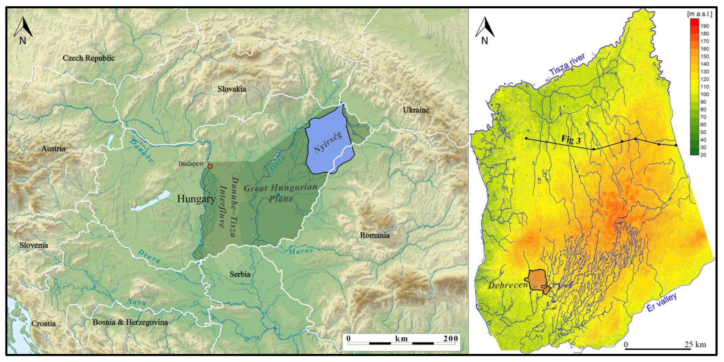
Figure 2.
Changes in specific groundwater reserves in the Danube-Tisza Interfluves, categorised by elevation (1960–2017), with a reference period of 1961–1965. From (Rakonczai és Fehér 2019) modified.
Figure 2.
Changes in specific groundwater reserves in the Danube-Tisza Interfluves, categorised by elevation (1960–2017), with a reference period of 1961–1965. From (Rakonczai és Fehér 2019) modified.
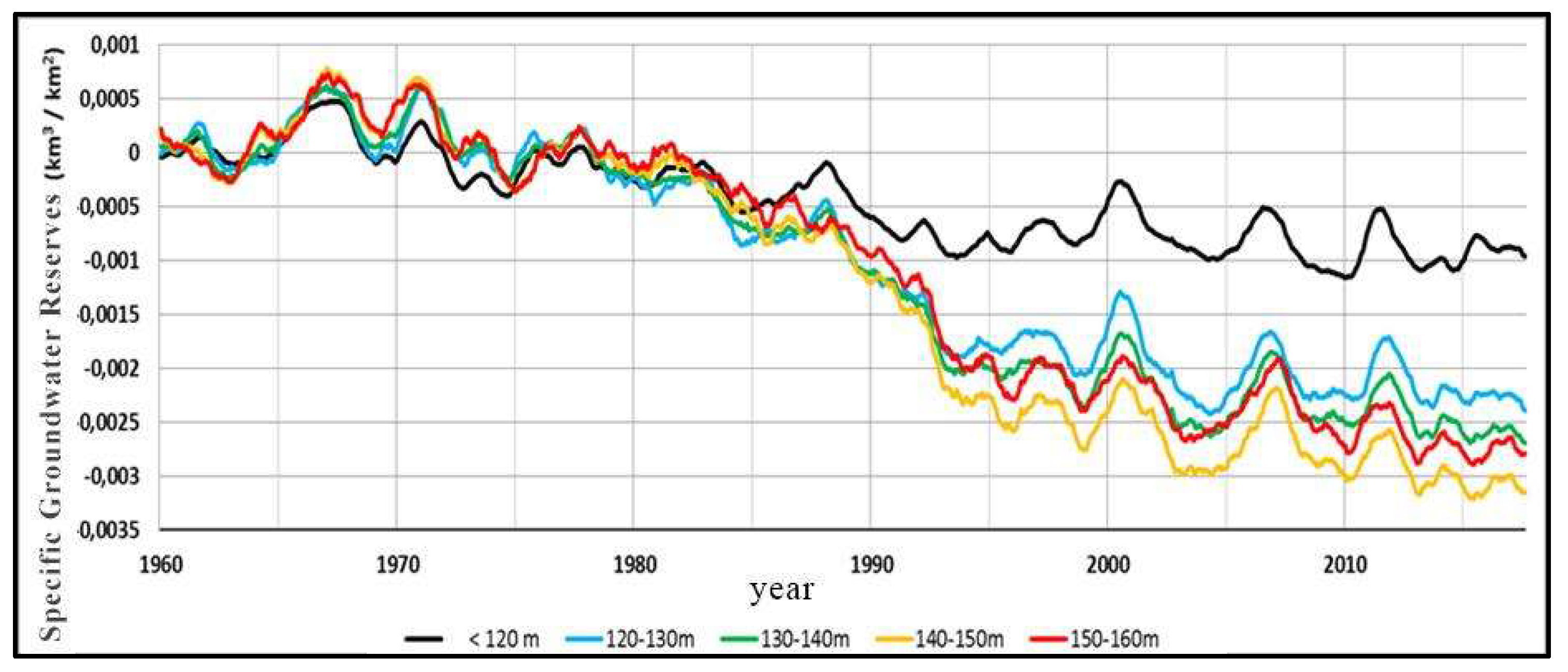
Figure 3.
West-East sedimentological section of Nyírség (section position see Figure 1b) (Püspöki 2013) modified.
Figure 3.
West-East sedimentological section of Nyírség (section position see Figure 1b) (Püspöki 2013) modified.
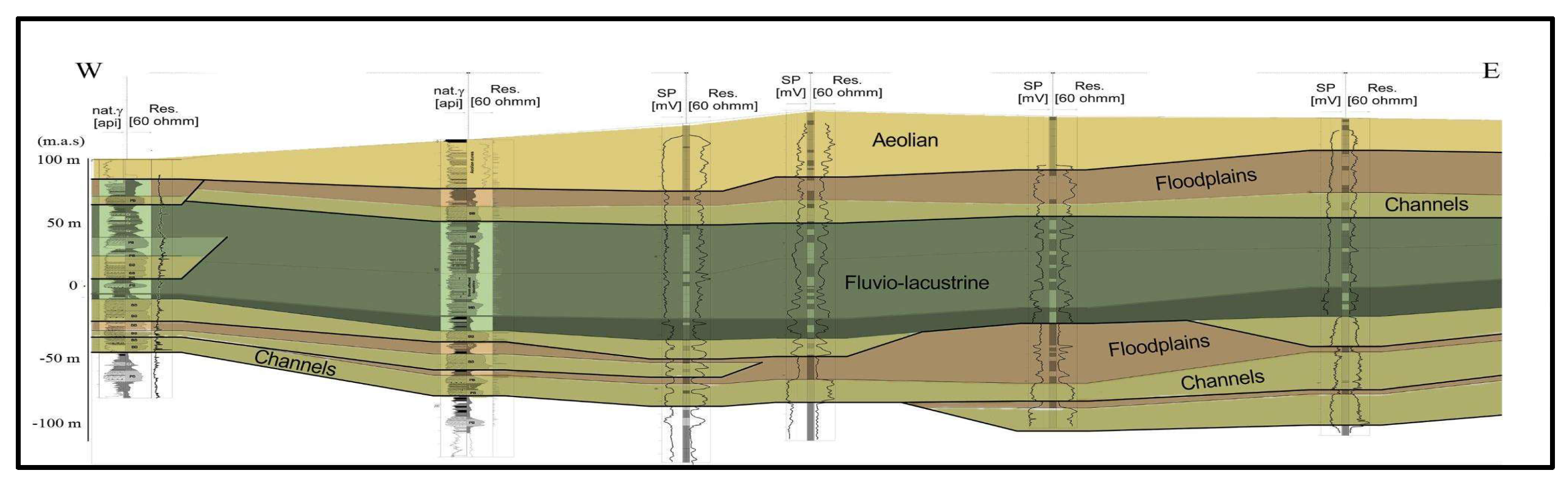
Figure 4.
Shallow groundwater level in Nyírség area (m a.s.l.).
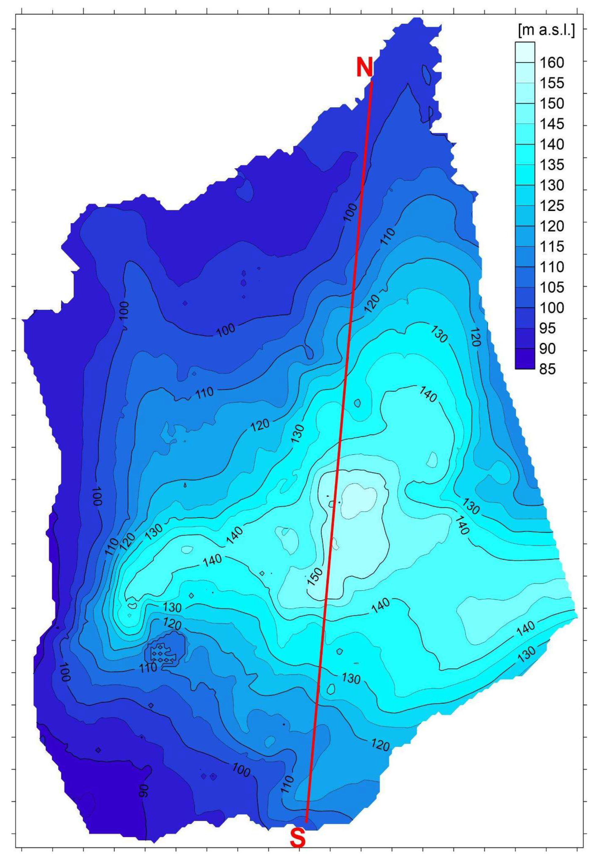
Figure 5.
The south-north groundwater flow system profile of the Pleistocene formations of the Nyírség, showing the location of the wells used (circles), and indicating the flow regime (Marton, 1981) modified.
Figure 5.
The south-north groundwater flow system profile of the Pleistocene formations of the Nyírség, showing the location of the wells used (circles), and indicating the flow regime (Marton, 1981) modified.
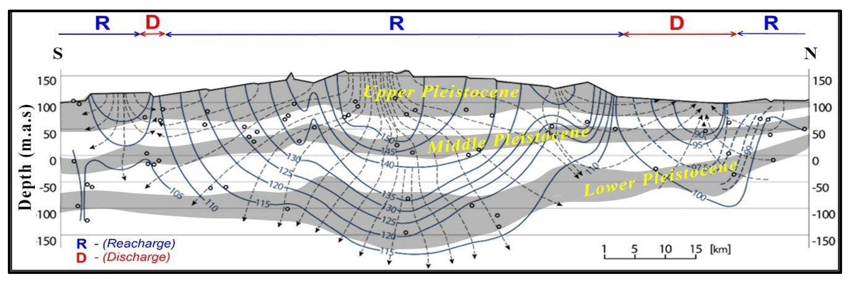
Figure 6.
Schematic overview of the hydroclimate workflow, in which CHIRPS daily precipitation and ERA5-Land hourly variables are clipped to the area of interest and processed in parallel to produce AOI-mean time series and multi-year spatial composites for consistent hydroclimate analysis.
Figure 6.
Schematic overview of the hydroclimate workflow, in which CHIRPS daily precipitation and ERA5-Land hourly variables are clipped to the area of interest and processed in parallel to produce AOI-mean time series and multi-year spatial composites for consistent hydroclimate analysis.
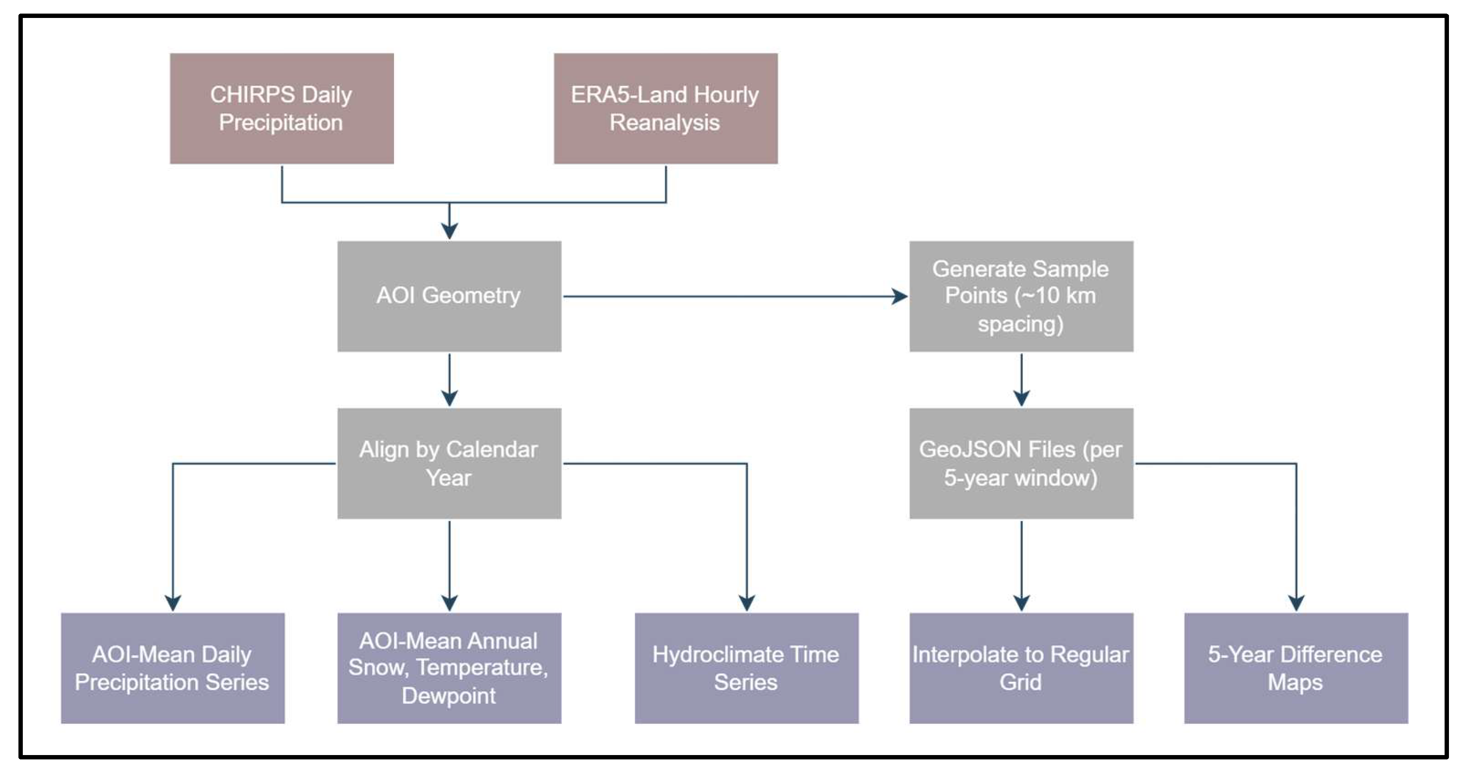
Figure 7.
Irrigated fields after merging neighbouring parcels using a 50 m buffer, forming consolidated field polygons used as the basis for subsequent analyses.
Figure 7.
Irrigated fields after merging neighbouring parcels using a 50 m buffer, forming consolidated field polygons used as the basis for subsequent analyses.
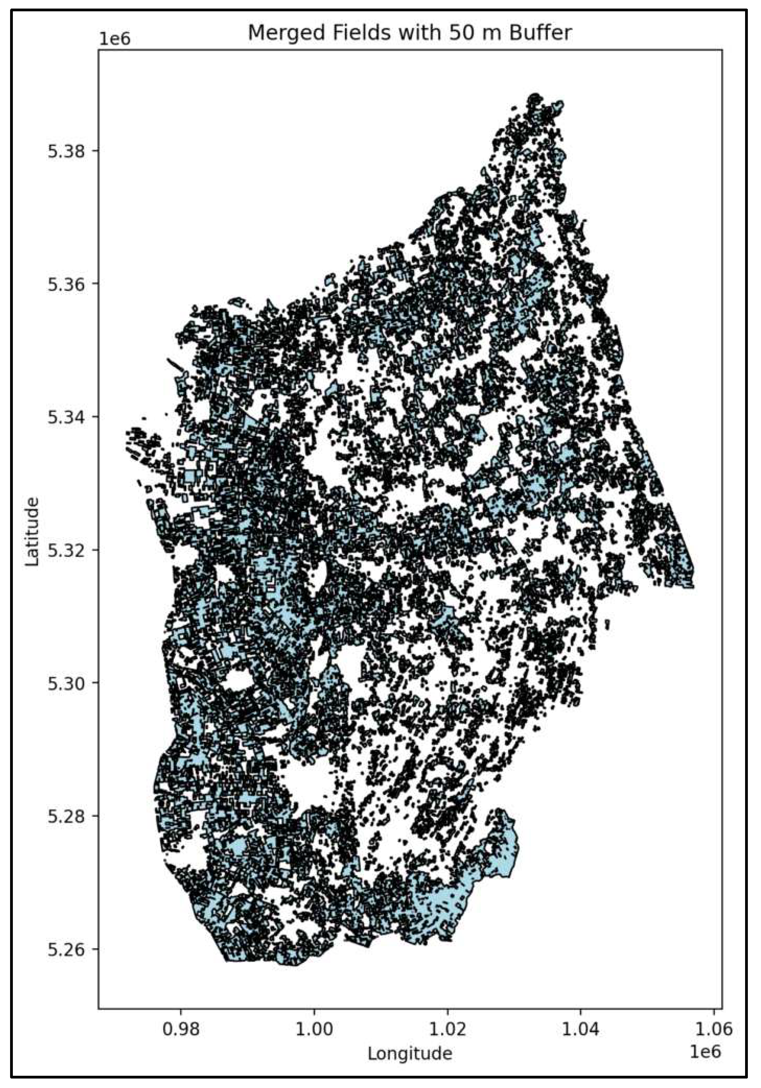
Figure 8.
Radial flow chart (Blue to Red direction) illustrating the integrated GEE–Python workflow, from AOI definition and buffered spatial sampling to cloud-based processing in Google Earth Engine and subsequent analysis and visualization in Python.
Figure 8.
Radial flow chart (Blue to Red direction) illustrating the integrated GEE–Python workflow, from AOI definition and buffered spatial sampling to cloud-based processing in Google Earth Engine and subsequent analysis and visualization in Python.
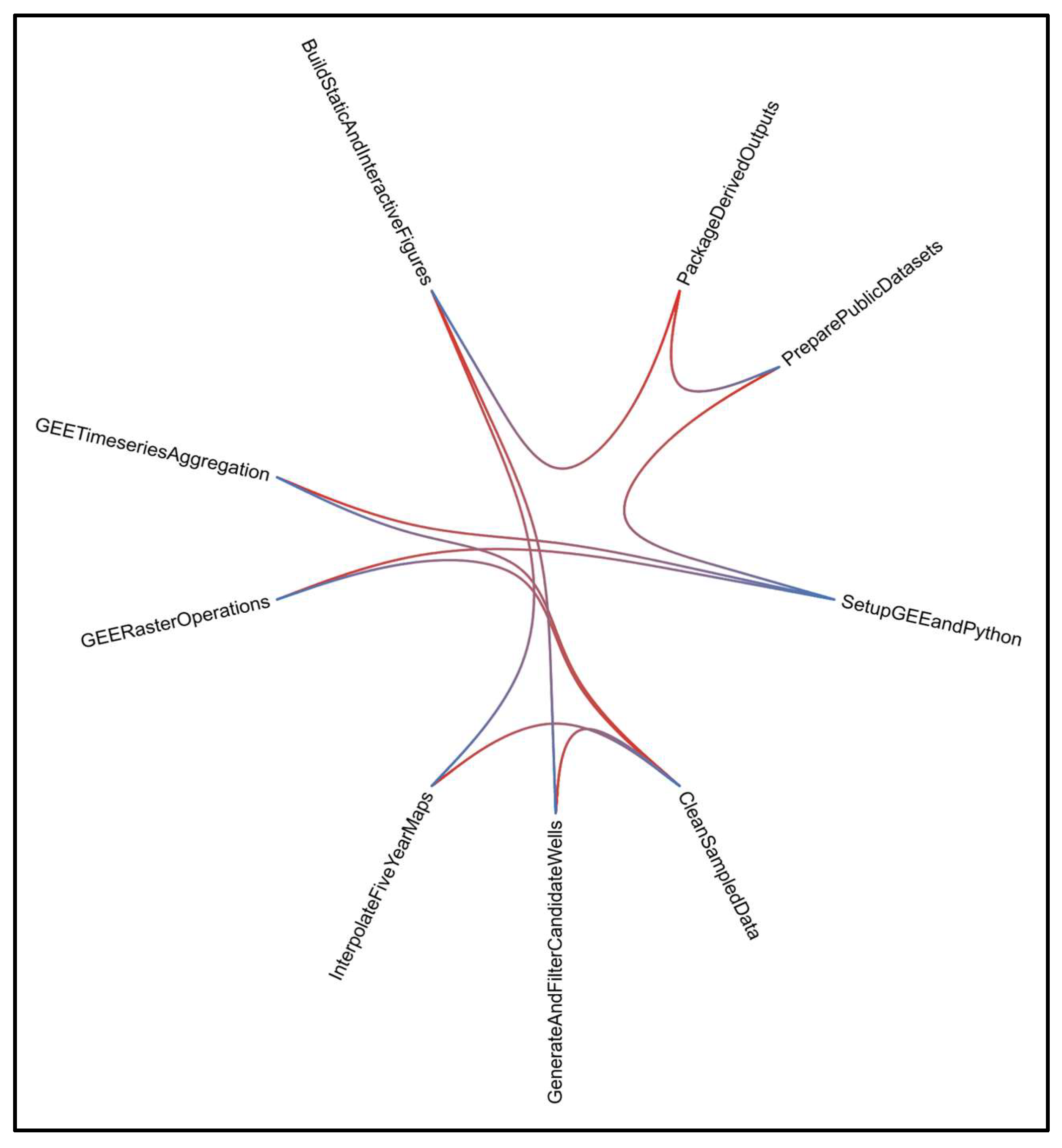
Figure 9.
Time-series of groundwater level data located between 110 and 120 m above sea level between 1970 and 2022, with the location of the wells indicated.
Figure 9.
Time-series of groundwater level data located between 110 and 120 m above sea level between 1970 and 2022, with the location of the wells indicated.
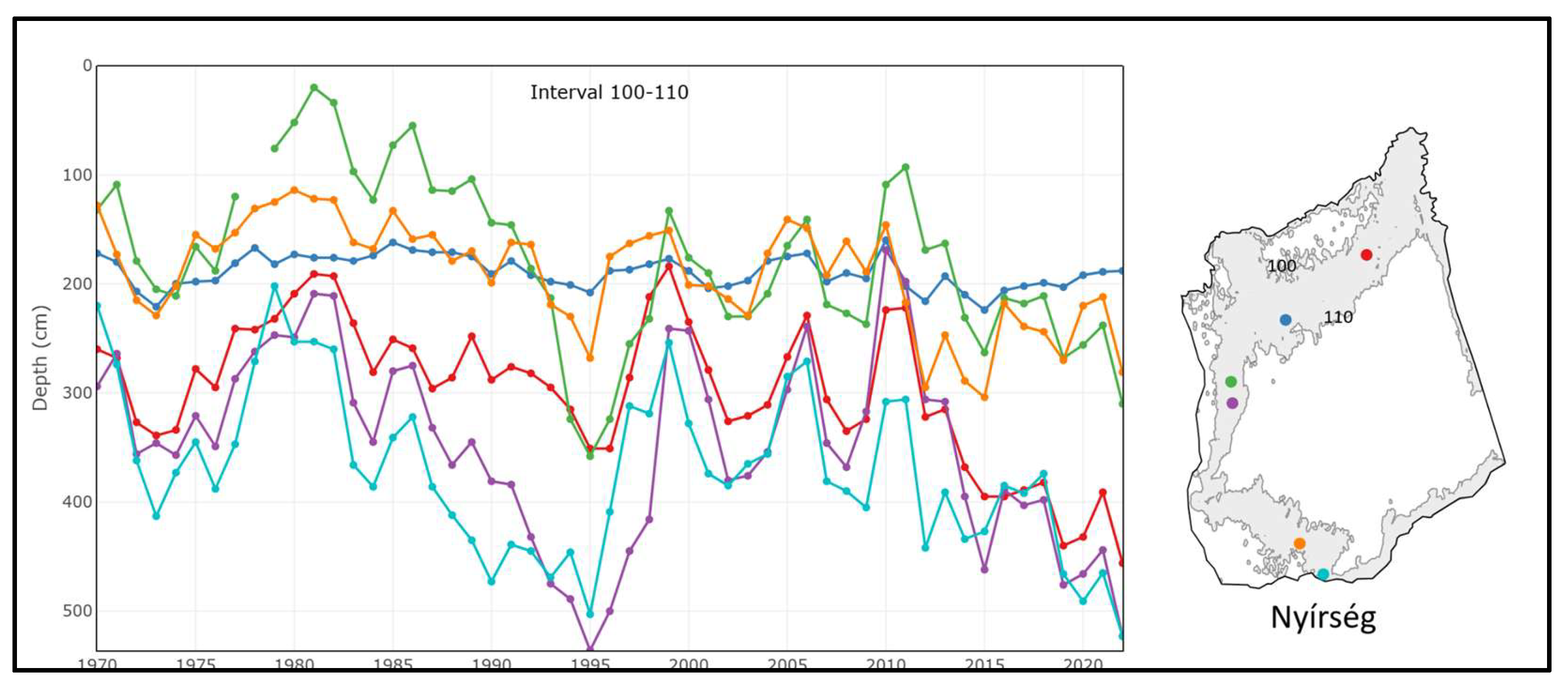
Figure 10.
Time-series of groundwater level data located between 140 and 150 m above sea level between 1970 and 2022, with the location of the wells indicated.
Figure 10.
Time-series of groundwater level data located between 140 and 150 m above sea level between 1970 and 2022, with the location of the wells indicated.
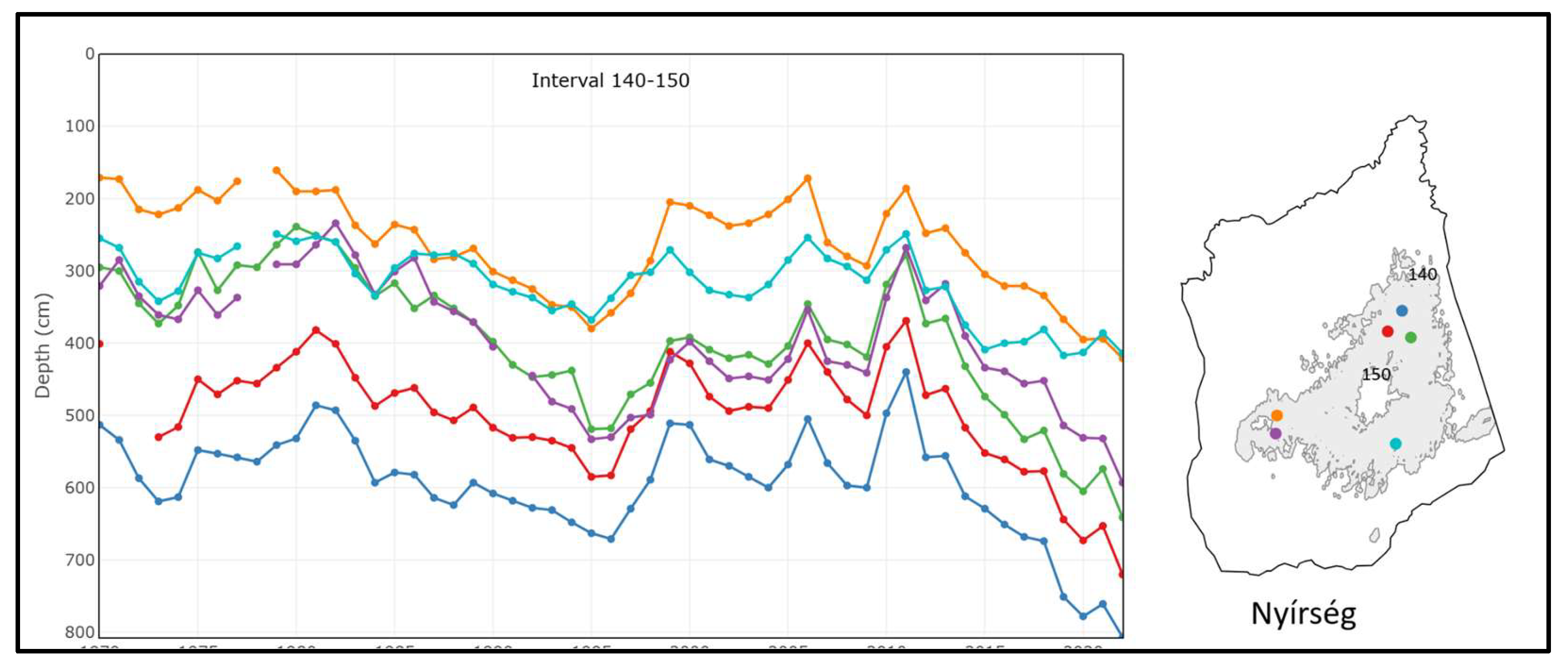
Figure 11.
The minimum depth of summer groundwater level below the surface in metres (2010) in the Nyírség region was calculated using Kriging.
Figure 11.
The minimum depth of summer groundwater level below the surface in metres (2010) in the Nyírség region was calculated using Kriging.
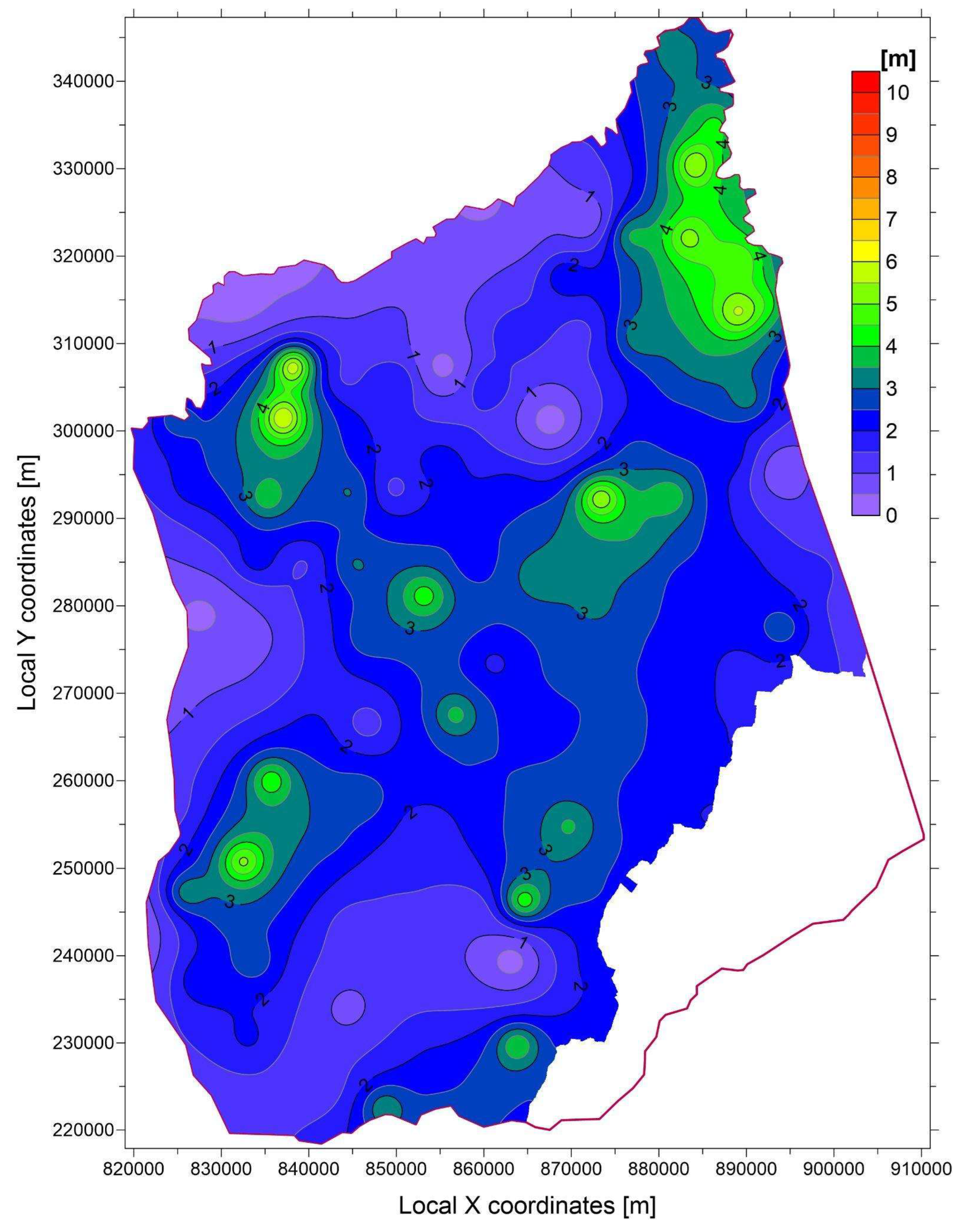
Figure 12.
The maximum depth of summer groundwater level below the surface in metres (2022) in the Nyírség region was calculated using Kriging.
Figure 12.
The maximum depth of summer groundwater level below the surface in metres (2022) in the Nyírség region was calculated using Kriging.
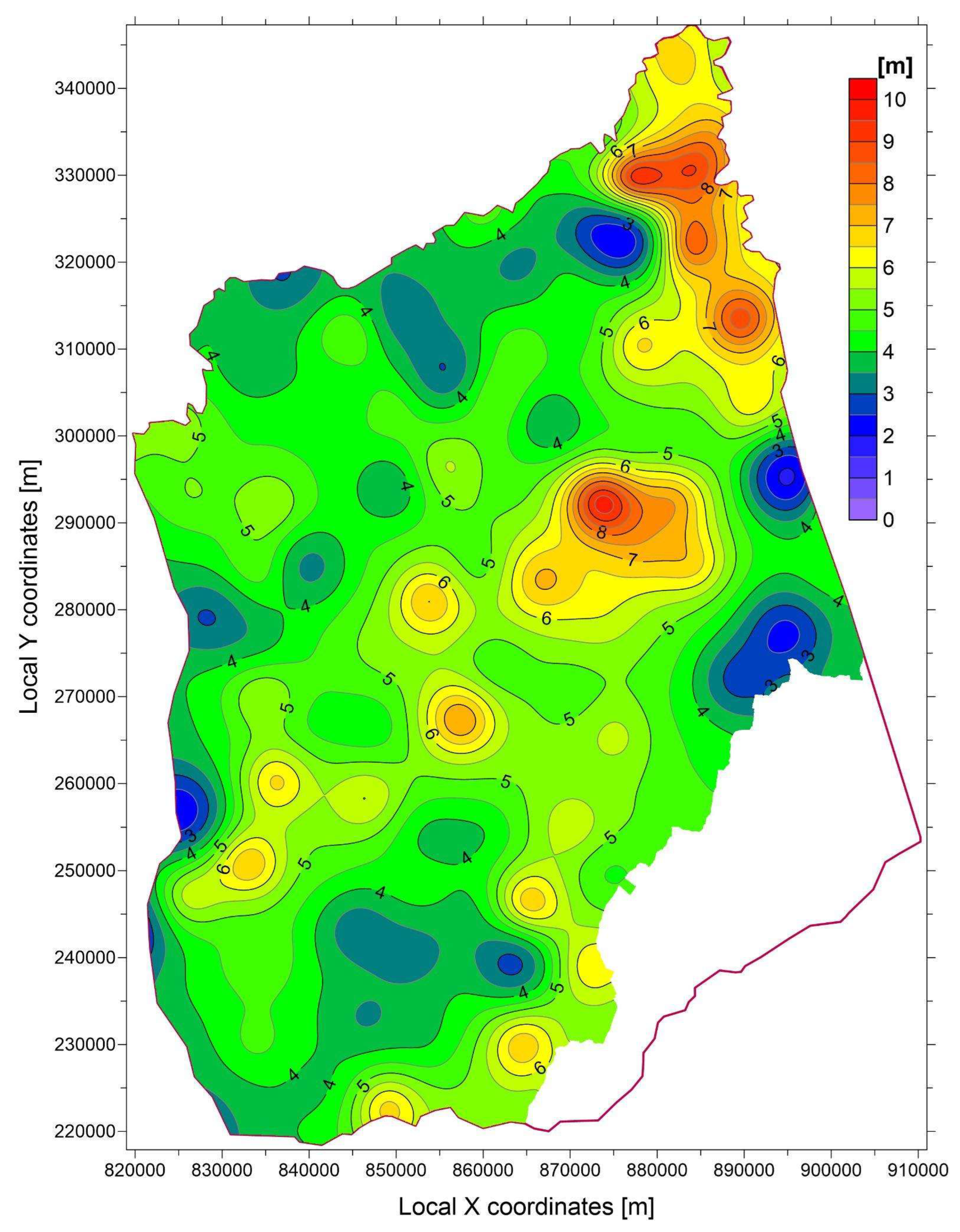
Figure 13.
The difference in metres between the minimum and maximum depths of the summer groundwater level (2022 and 2010) below the surface in the Nyírség region.
Figure 13.
The difference in metres between the minimum and maximum depths of the summer groundwater level (2022 and 2010) below the surface in the Nyírség region.
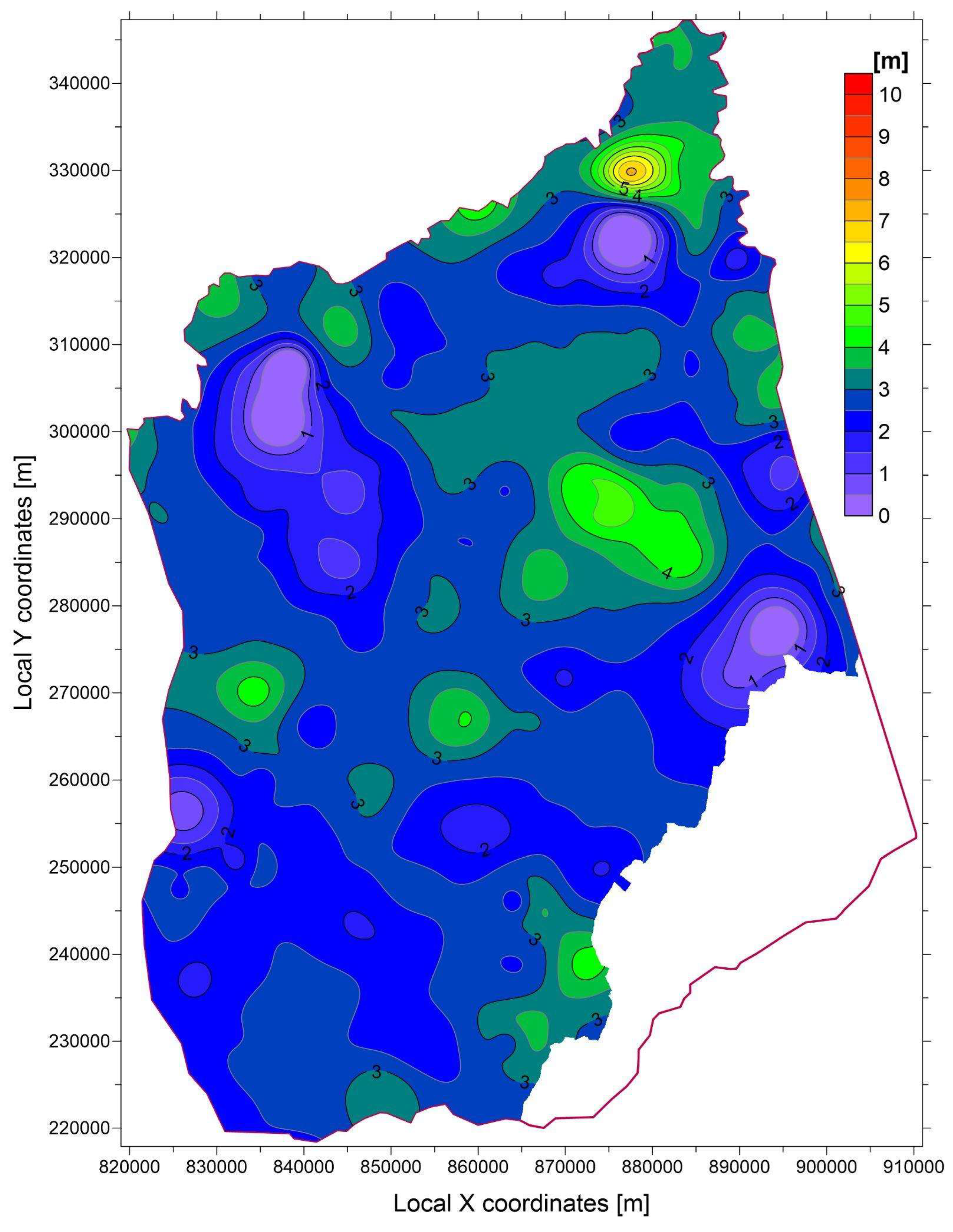
Figure 14.
Spatial distribution of wells in the Nyírség region. Red points show legal wells, while blue points indicate generated potential illegal wells.
Figure 14.
Spatial distribution of wells in the Nyírség region. Red points show legal wells, while blue points indicate generated potential illegal wells.
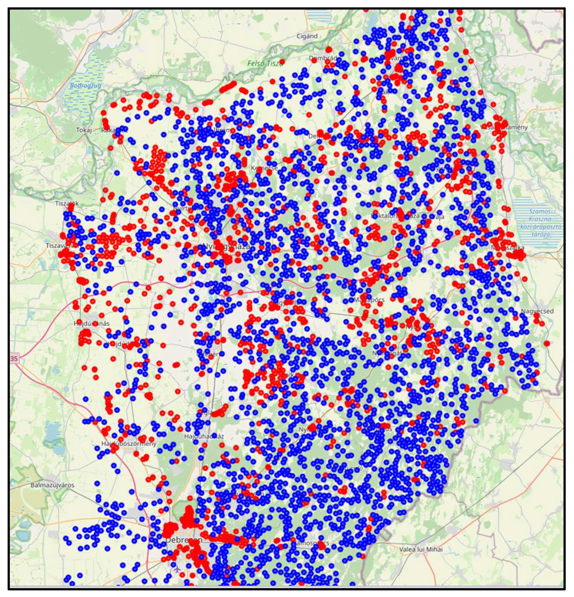
Figure 15.
Annual precipitation and heavy-rain contribution (>25 mm day⁻¹) with snow depth and air temperature. Left axis bars show total annual precipitation (blue) and heavy-rain contribution (>25 mm day⁻¹, red). Right axis lines display annual mean snow depth (scaled ×250) and 2 m air temperature (scaled ×1), illustrating the relationship between heavy rainfall and cryospheric/thermal conditions.
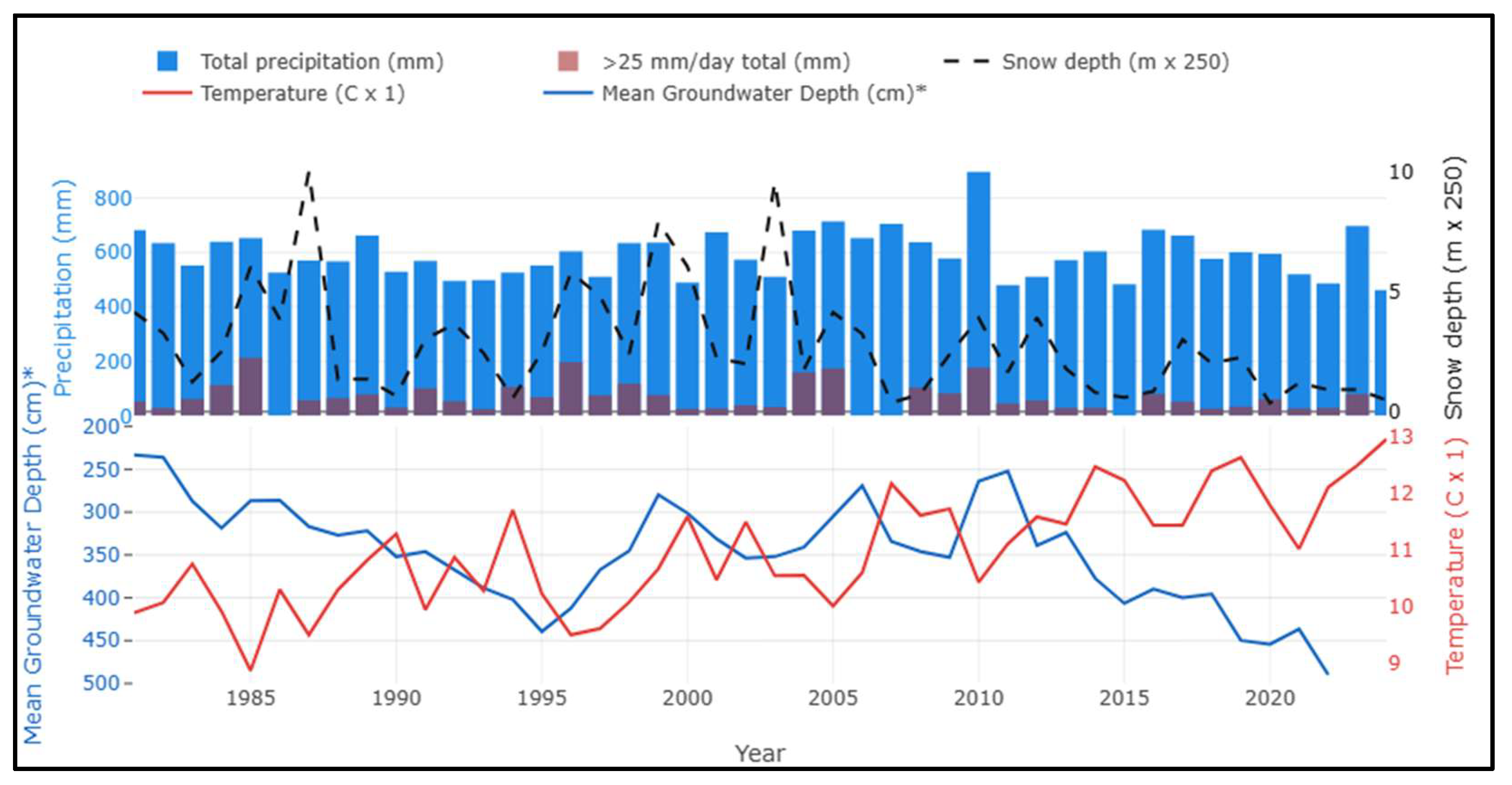
Figure 16.
Bias-adjusted 2 m air temperature projection for the study area under RCP4.5 and RCP8.5 (30-year, daily, moving-average adjustment).
Figure 16.
Bias-adjusted 2 m air temperature projection for the study area under RCP4.5 and RCP8.5 (30-year, daily, moving-average adjustment).
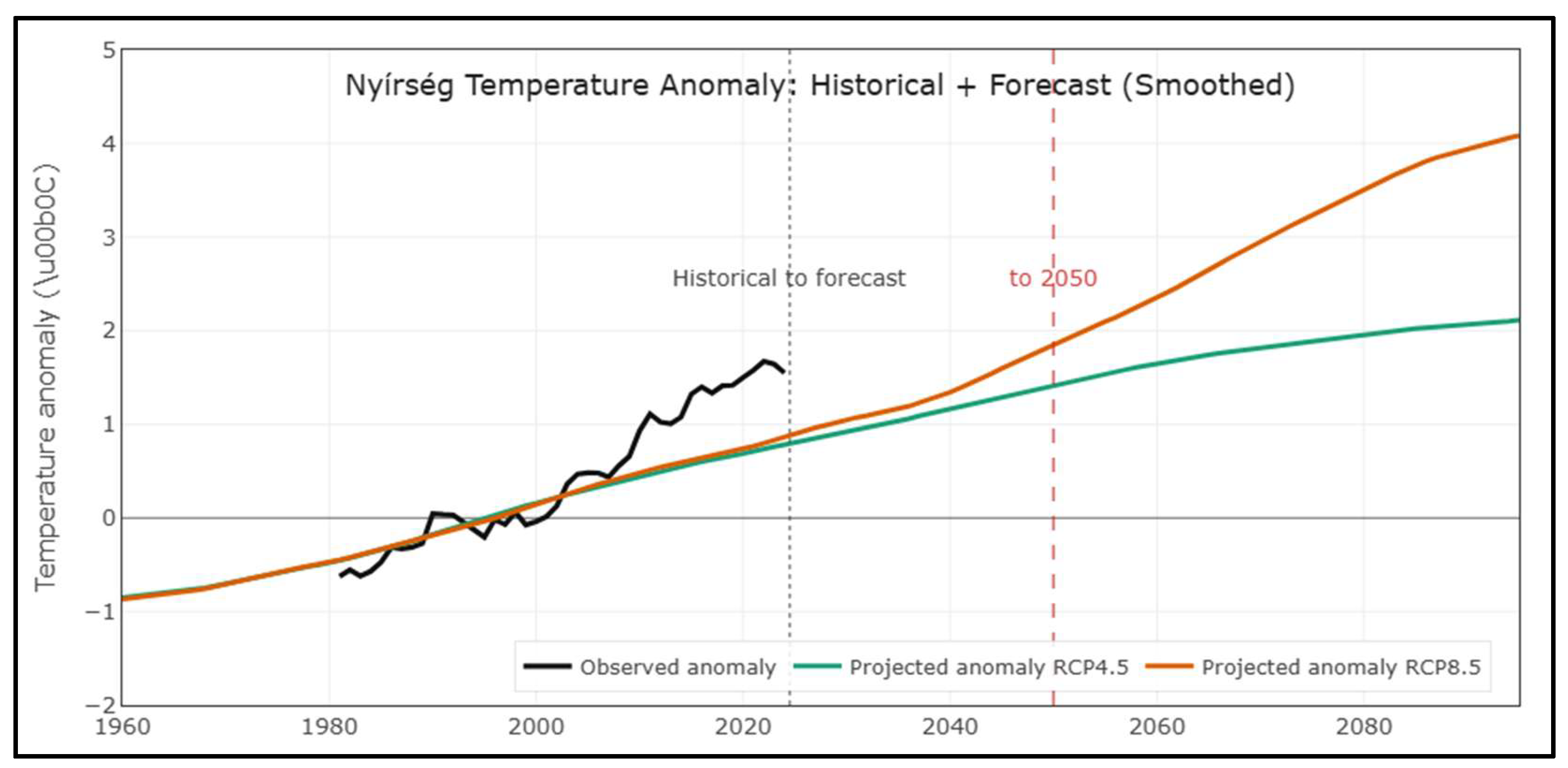
Figure 17.
The model's grid with rivers and the trace of vertical section.
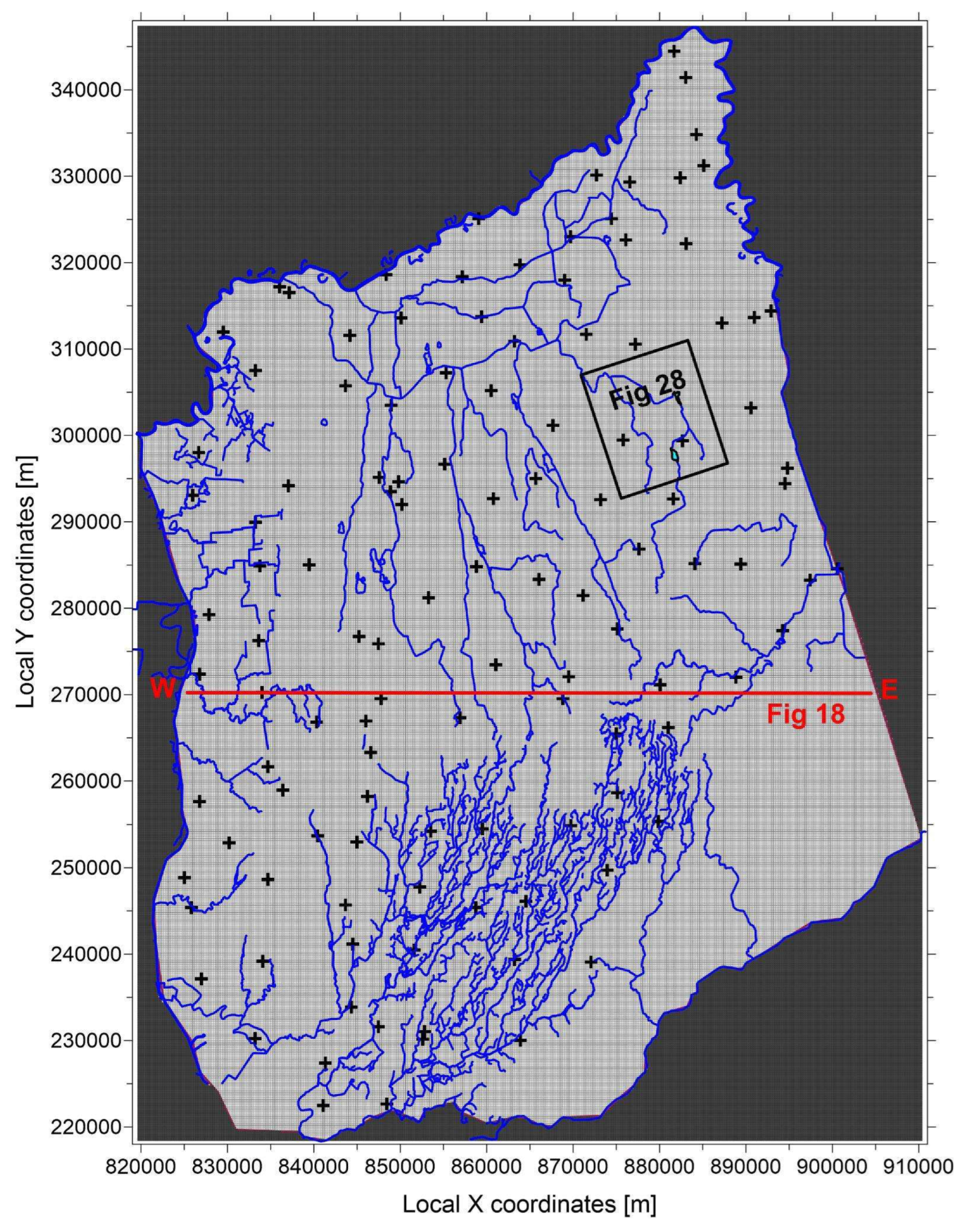
Figure 18.
The west-east section of the model with equipotential lines [m].
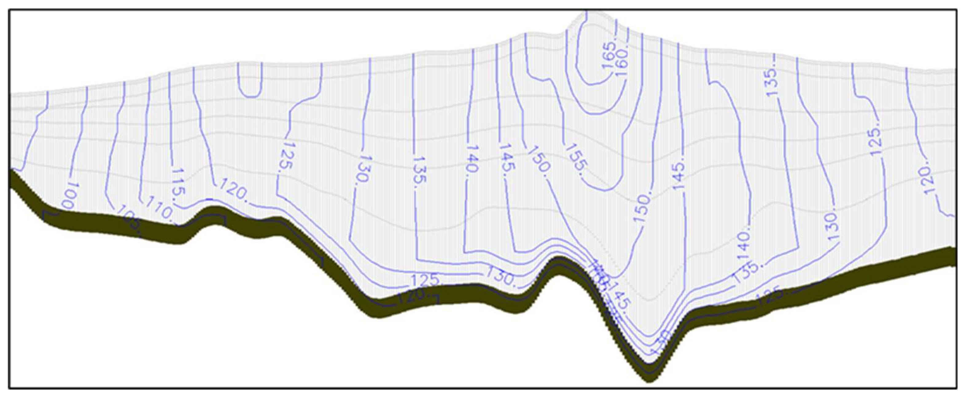
Figure 19.
Infiltration values [mm/year] in the modeled area.
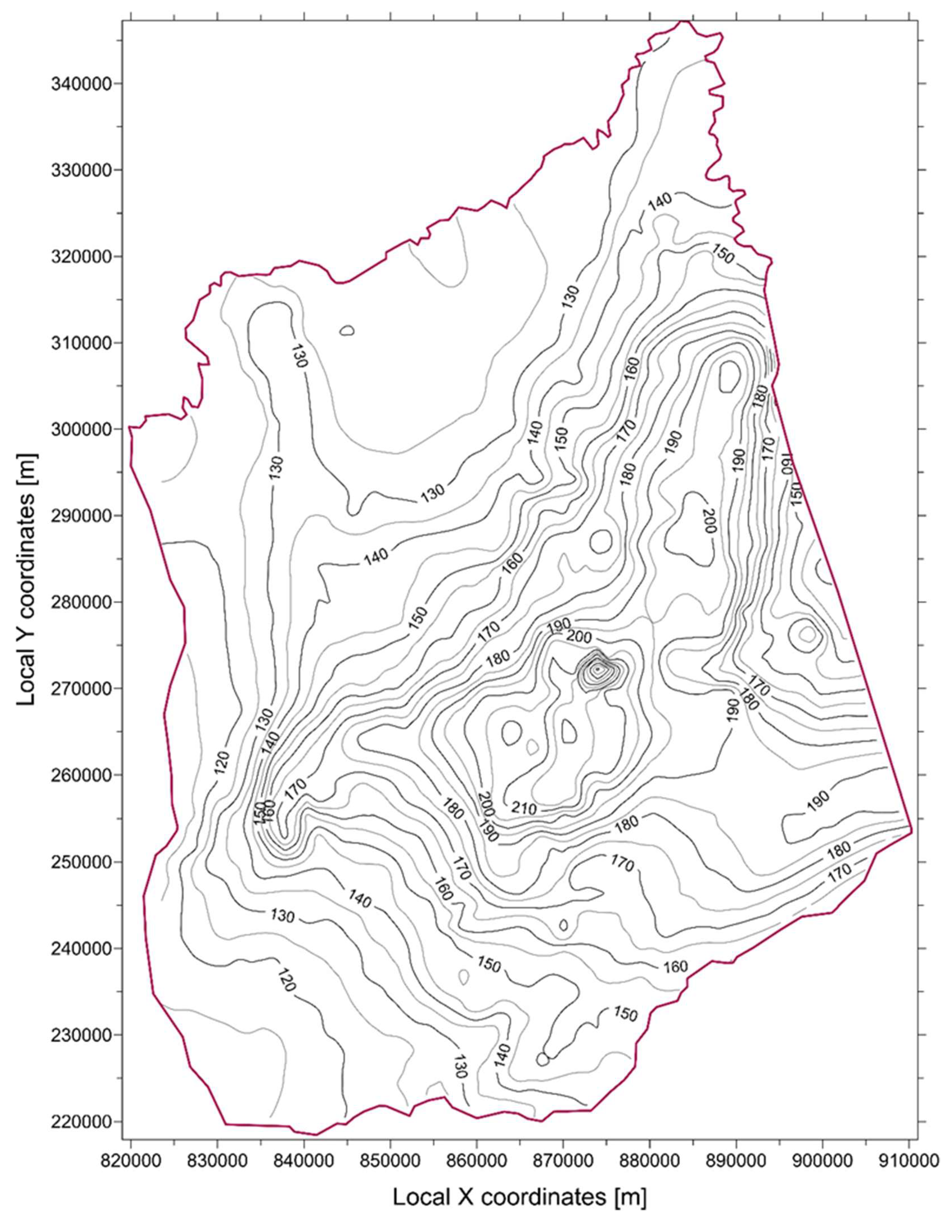
Figure 20.
Correlation and variance between observed and calculated water levels in monitoring wells following calibration during the dry season.
Figure 20.
Correlation and variance between observed and calculated water levels in monitoring wells following calibration during the dry season.
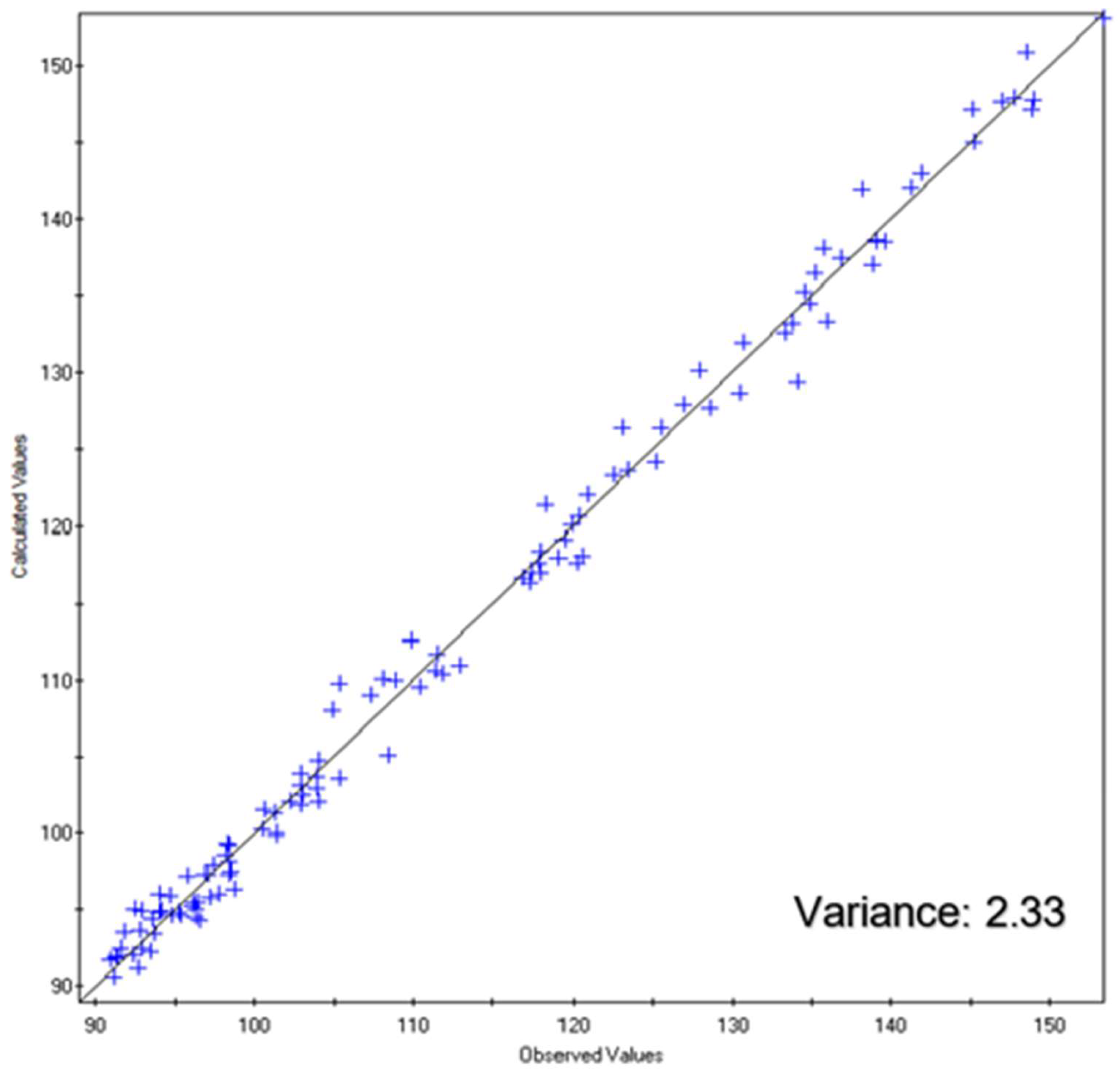
Figure 21.
Correlation and variance between observed and calculated water levels in monitoring wells following calibration during the wet season.
Figure 21.
Correlation and variance between observed and calculated water levels in monitoring wells following calibration during the wet season.
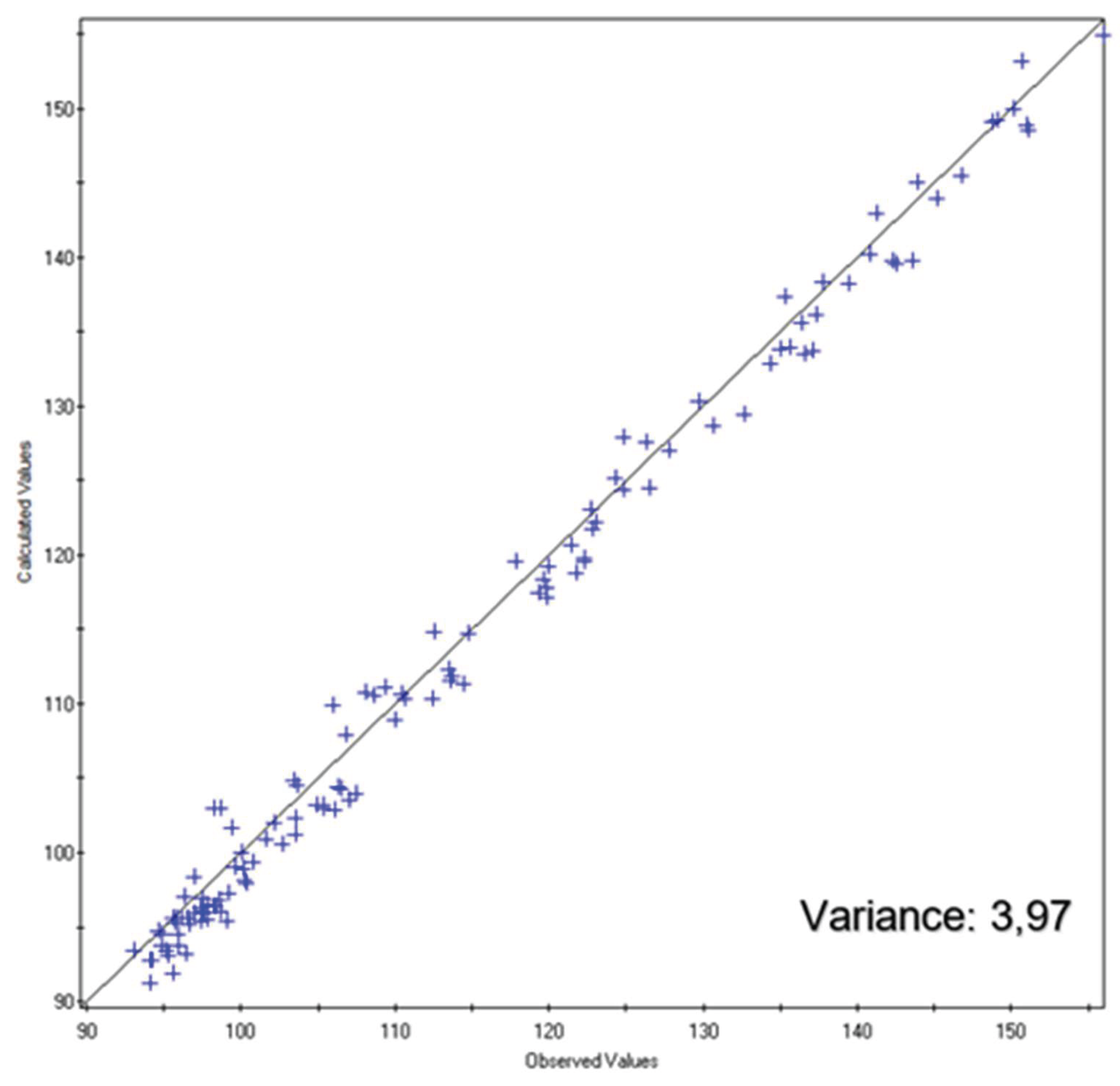
Figure 22.
Shallow groundwater level in Nyírség area in 2022 (m a.s.l.).
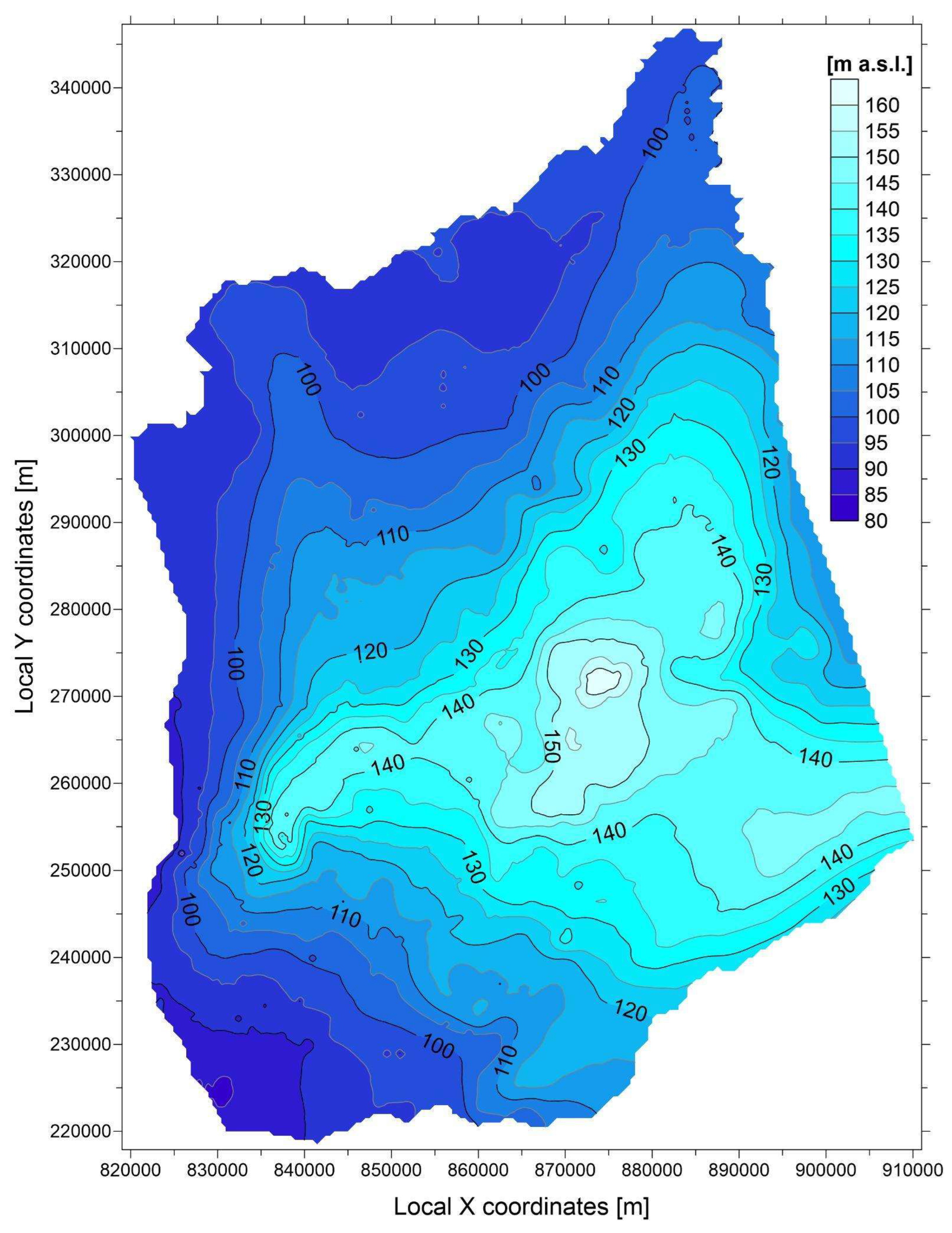
Figure 23.
The extent of shallow groundwater level decline (in meters) in the Nyírség region between 2010 and 2022.
Figure 23.
The extent of shallow groundwater level decline (in meters) in the Nyírség region between 2010 and 2022.
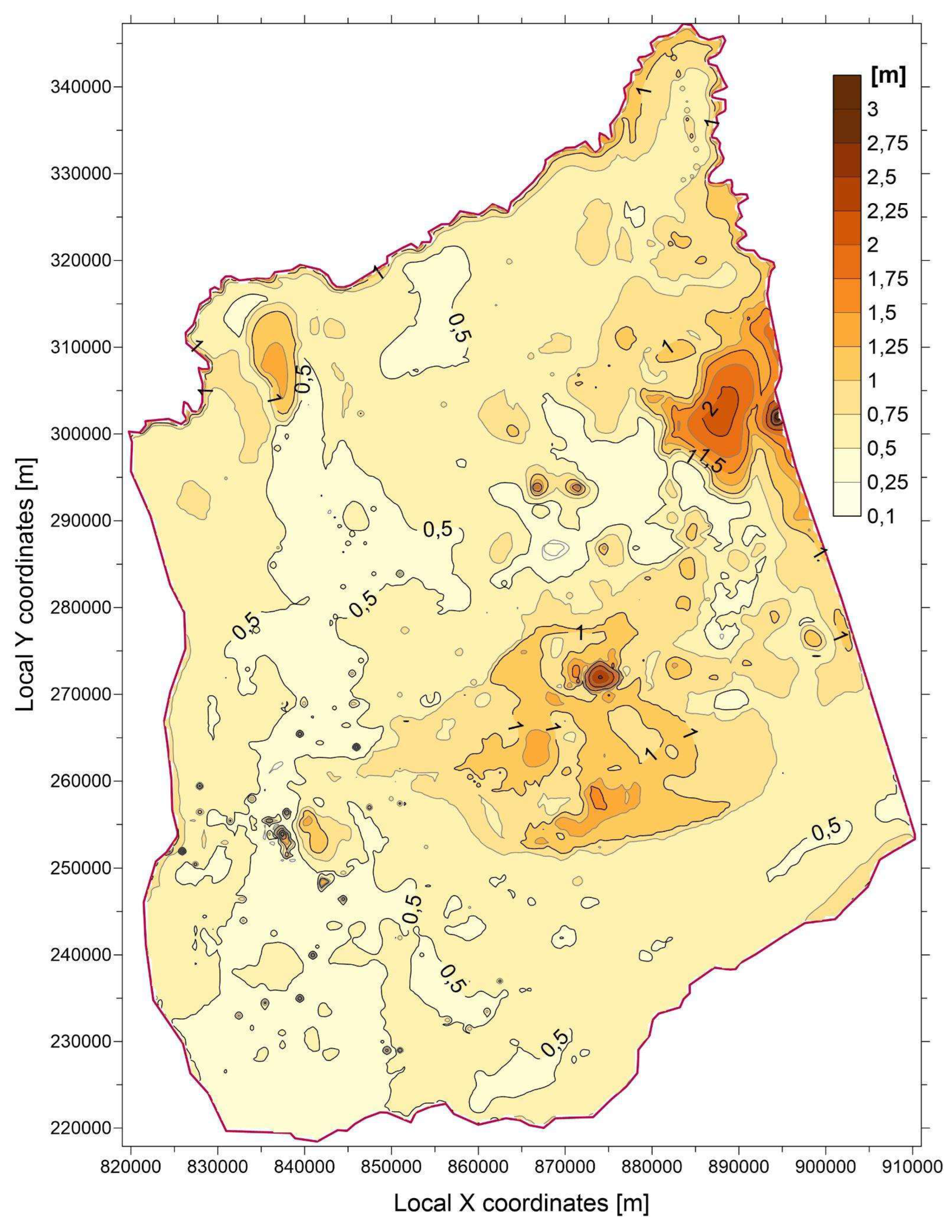
Figure 24.
The extent of the decline in shallow groundwater levels (in metres) in the Nyírség region under extreme drought climatic conditions in 2050.
Figure 24.
The extent of the decline in shallow groundwater levels (in metres) in the Nyírség region under extreme drought climatic conditions in 2050.
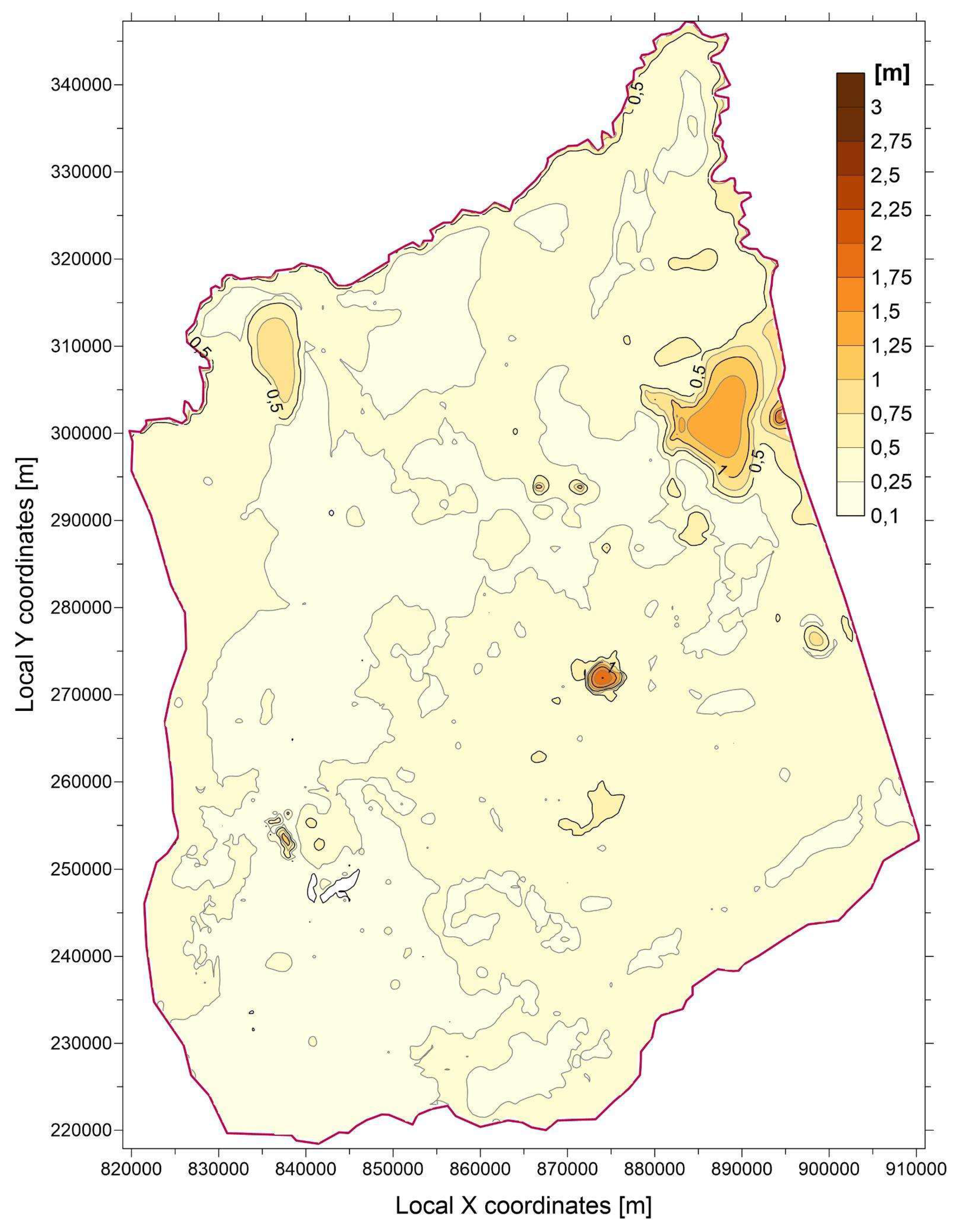
Figure 25.
The extent of the decline in shallow groundwater levels (in metres) in the Nyírség region in the event of a 20% increase in water withdrawal.
Figure 25.
The extent of the decline in shallow groundwater levels (in metres) in the Nyírség region in the event of a 20% increase in water withdrawal.
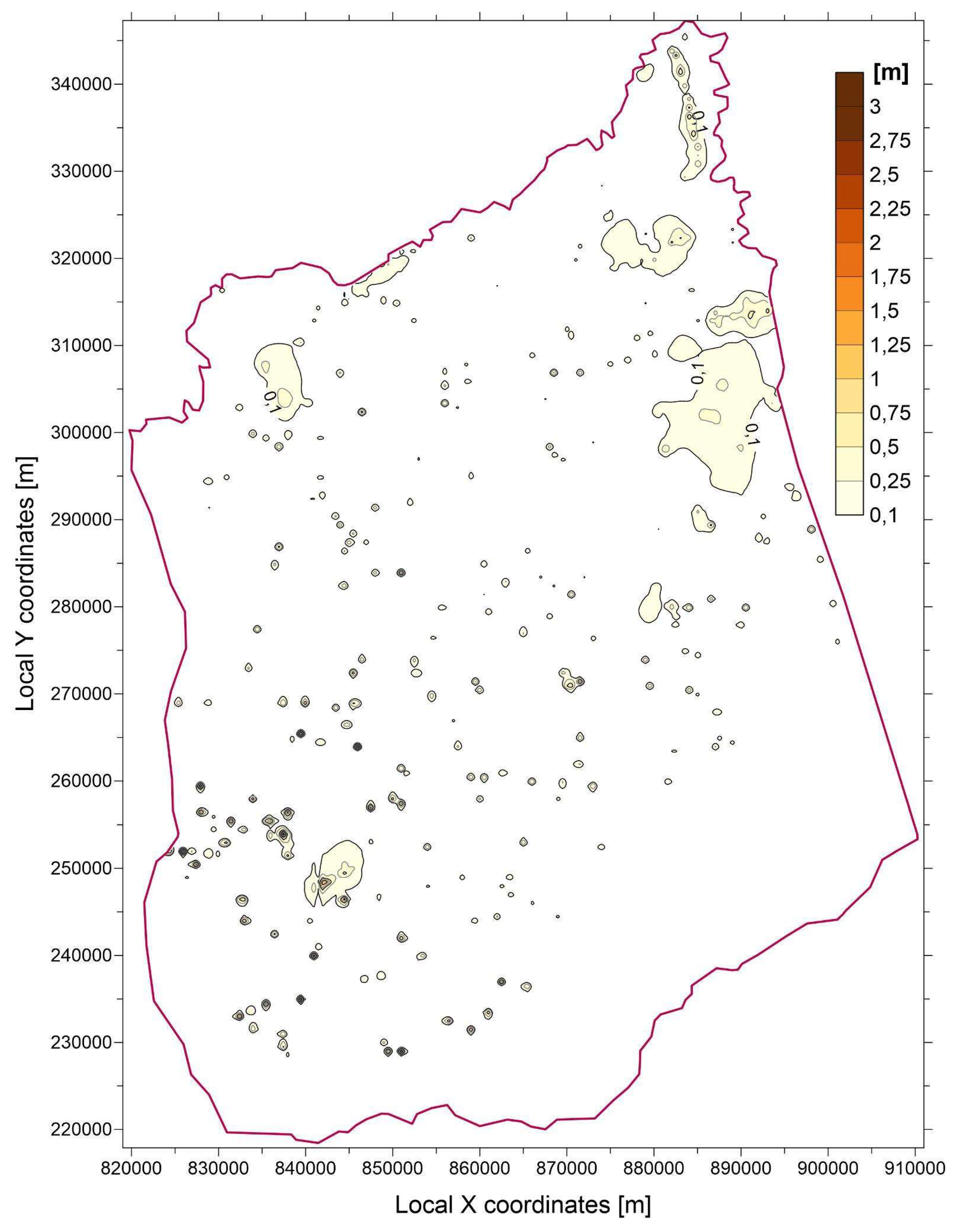
Figure 26.
The extent of the decline in groundwater level of middle Pleistocene aquifer (model layer 4) in metres in the Nyírség region under continuous extreme drought climatic conditions in 2050.
Figure 26.
The extent of the decline in groundwater level of middle Pleistocene aquifer (model layer 4) in metres in the Nyírség region under continuous extreme drought climatic conditions in 2050.
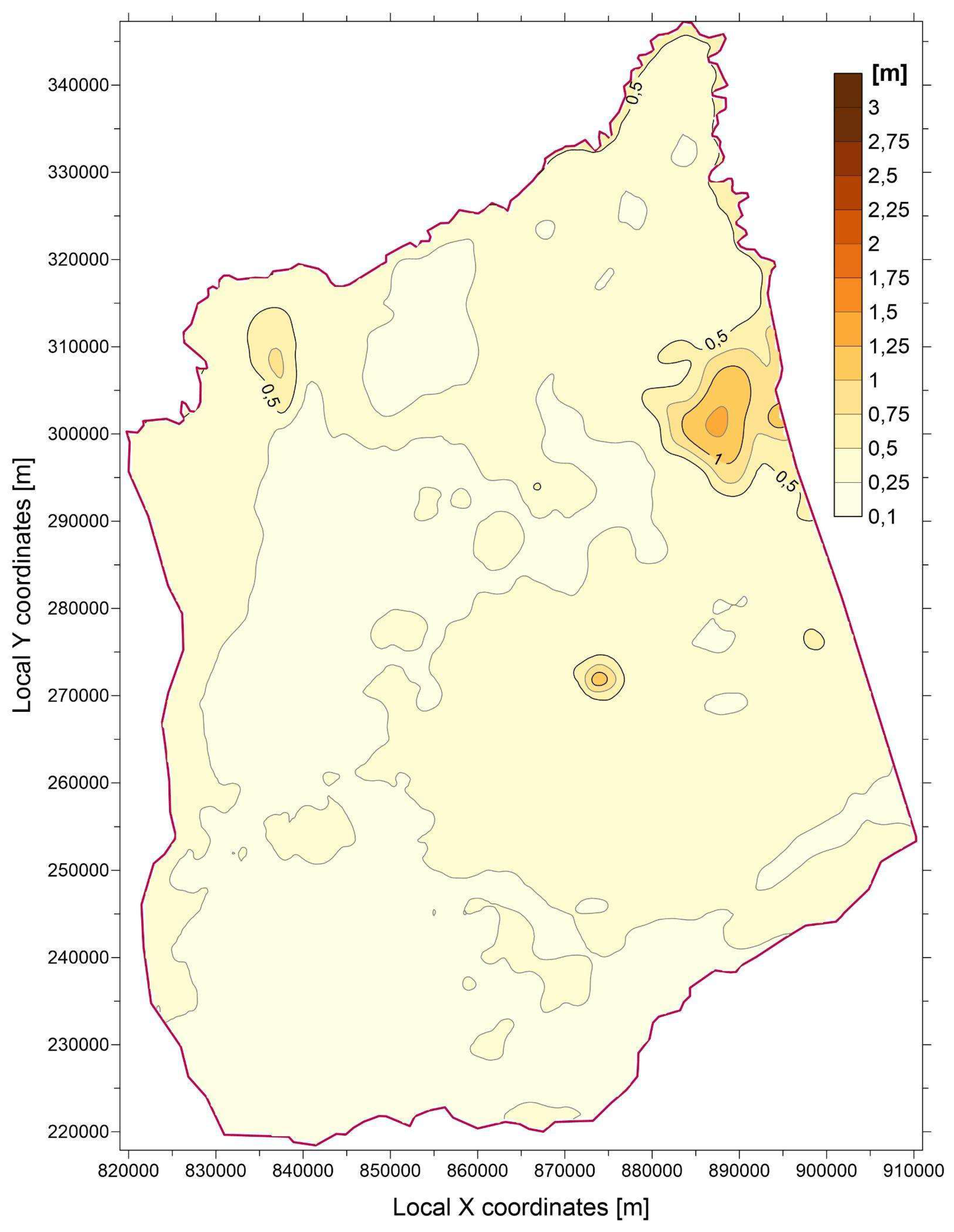
Figure 27.
The extent of the decline in groundwater level of lower Pleistocene aquifer (model layer 6) in metres in the Nyírség region under continuous extreme drought climatic conditions in 2050.
Figure 27.
The extent of the decline in groundwater level of lower Pleistocene aquifer (model layer 6) in metres in the Nyírség region under continuous extreme drought climatic conditions in 2050.
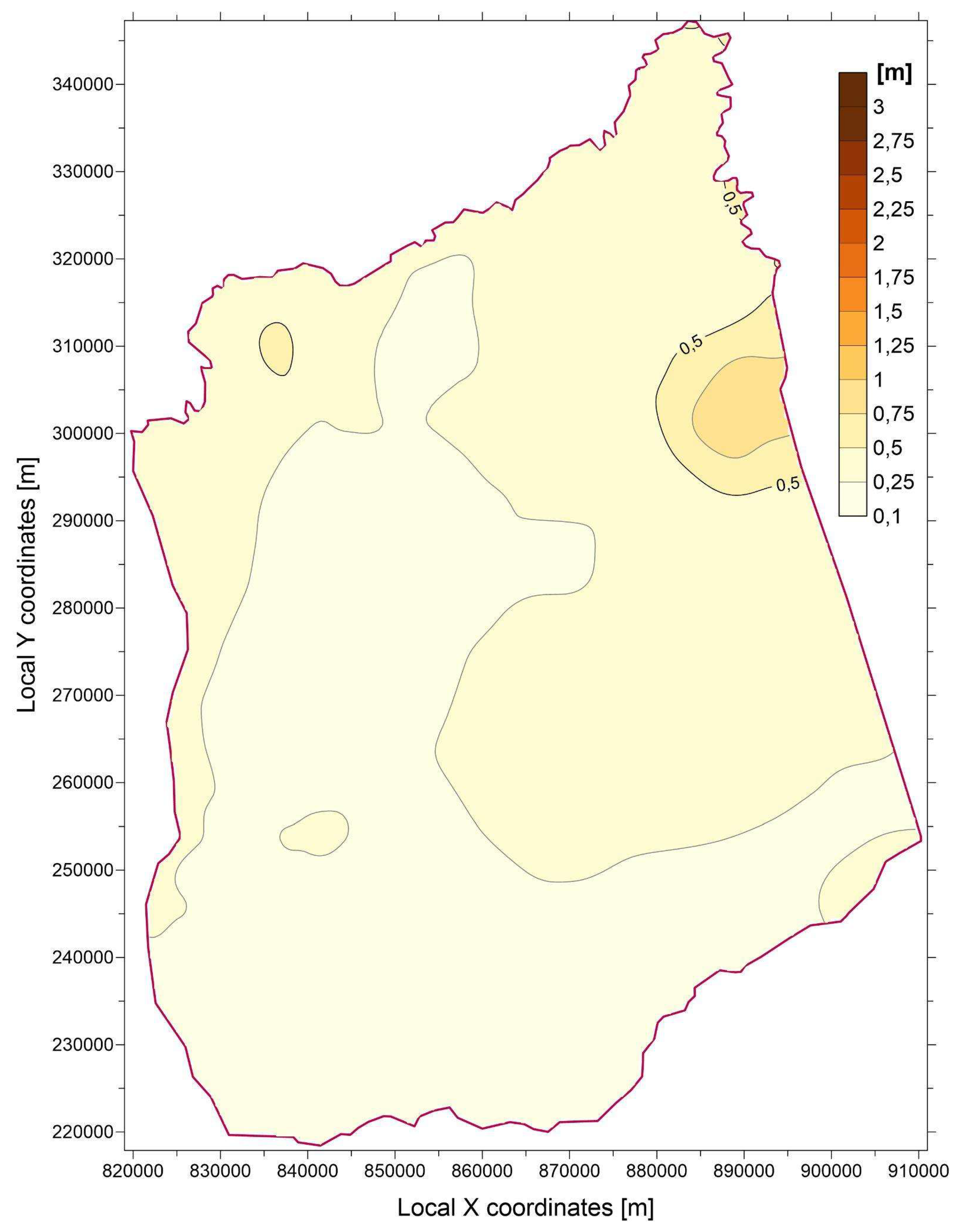
Figure 28.
The terrain of the model area was examined in detail to show the channels and lakes that were taken into account in the simulation (See Figure 17 for the location of the area).
Figure 28.
The terrain of the model area was examined in detail to show the channels and lakes that were taken into account in the simulation (See Figure 17 for the location of the area).
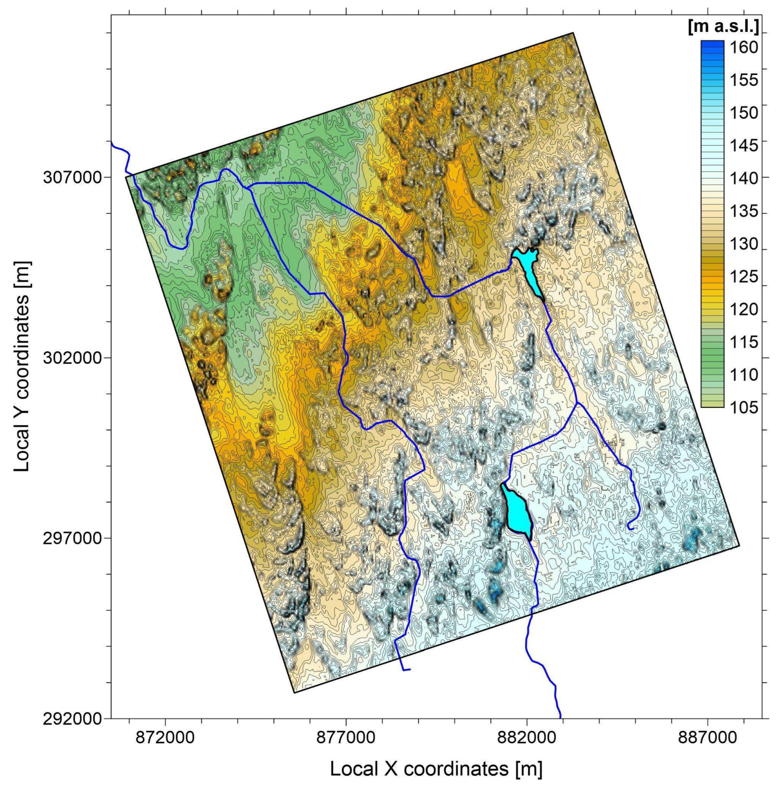
Figure 29.
The value of groundwater depression due to permanent water recharge in channels and lakes (Negative values indicate a rise in water level.).
Figure 29.
The value of groundwater depression due to permanent water recharge in channels and lakes (Negative values indicate a rise in water level.).
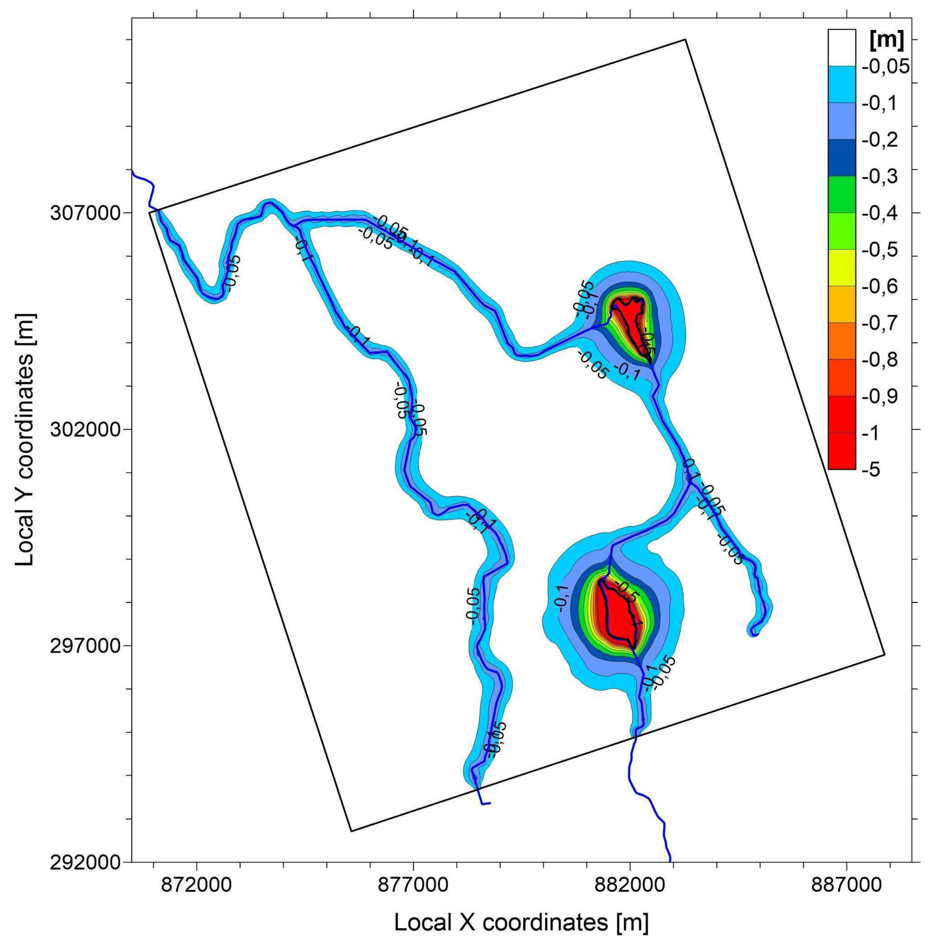
Figure 30.
The value of groundwater depression due to water recharge in channels and lakes in the case of transient simulation: a) after the end of the first replenishment period; b) after the end of the third replenishment period; c) after the end of the fifth replenishment period; c) after the end of the fifth dry period (Negative values indicate a rise in water level.) The crosses indicate the location of observation wells.
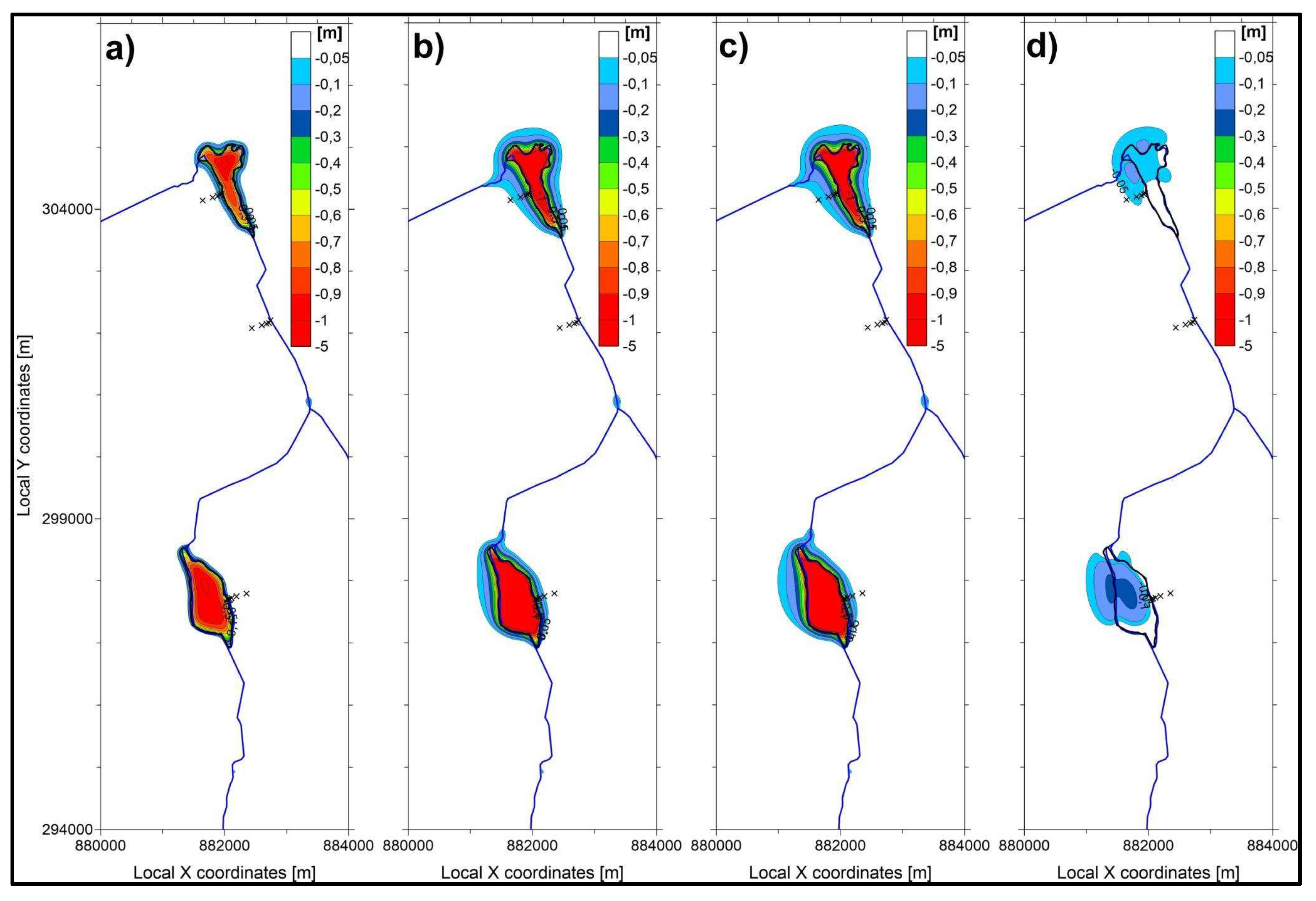
Figure 31.
Water level changes in virtual observation wells at different distances from the transient water replenishment location over time: (A) near the northern lake; (B) near the southern lake; (C) near the channel between the lakes (See the location of the observation wells on Figure 30).
Figure 31.
Water level changes in virtual observation wells at different distances from the transient water replenishment location over time: (A) near the northern lake; (B) near the southern lake; (C) near the channel between the lakes (See the location of the observation wells on Figure 30).
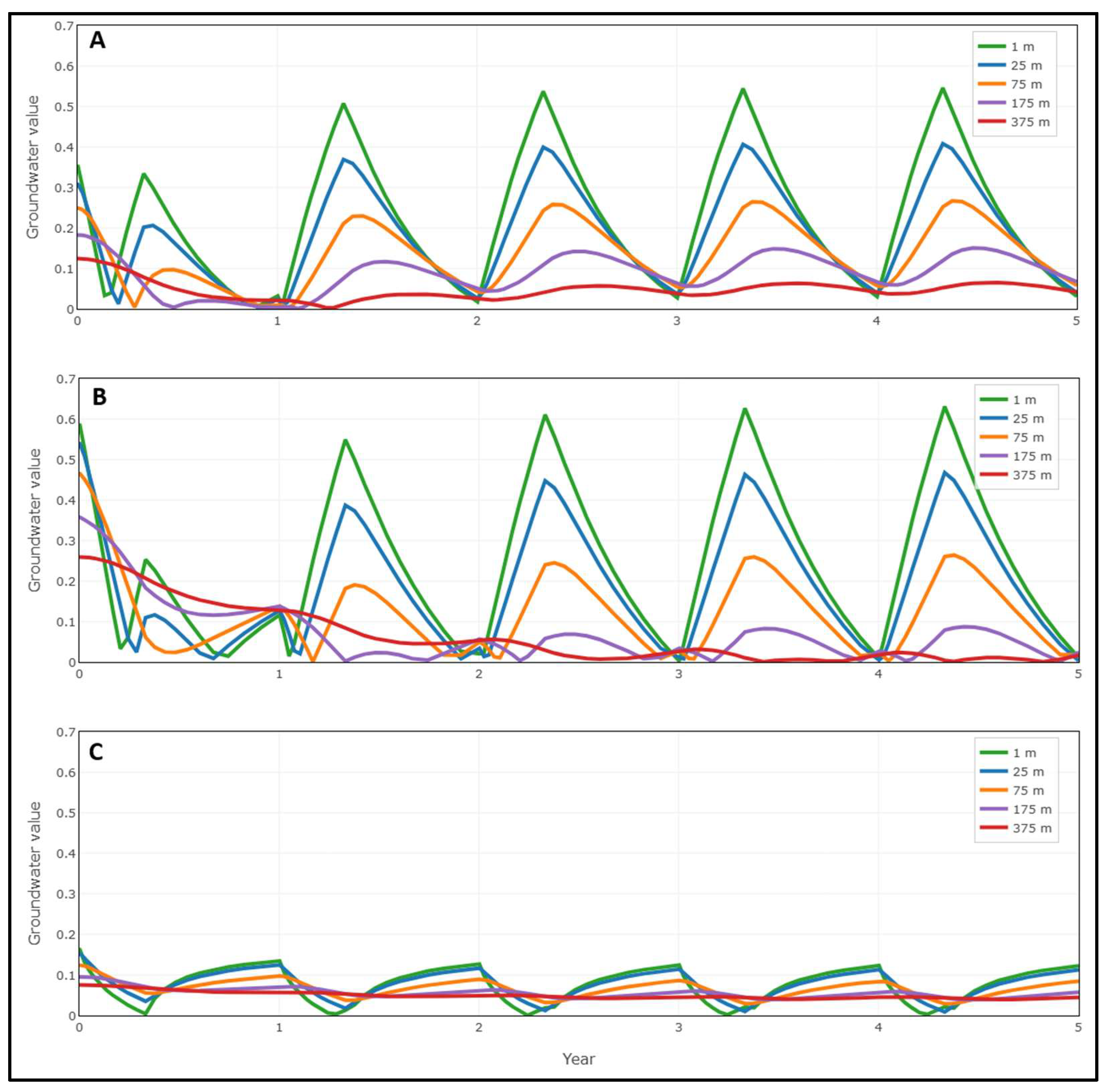
Figure 32.
The value of groundwater depression due to permanent water recharge in channels and lakes (Negative values indicate a rise in water level.).
Figure 32.
The value of groundwater depression due to permanent water recharge in channels and lakes (Negative values indicate a rise in water level.).
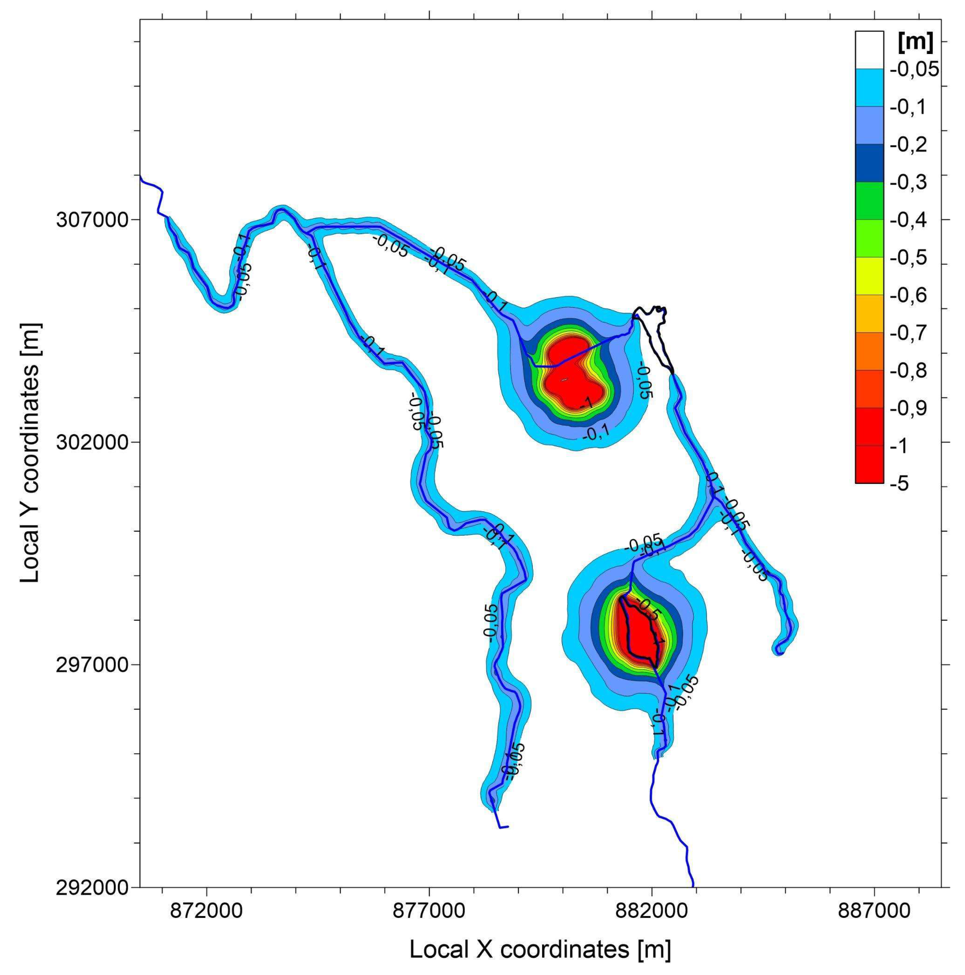

Table 1.
Overview of primary datasets and processing steps underlying each hydroclimate dashboard view.
Table 1.
Overview of primary datasets and processing steps underlying each hydroclimate dashboard view.
| View | Primary dataset(s) | Processing summary | Notes |
|---|---|---|---|
| Daily Precipitation Trends | CHIRPS daily precipitation (UCSB-CHG/CHIRPS/DAILY) | cached_daily_stats pulls daily AOI means; user-selected date range and rolling window generate raw vs smoothed series | Requires analysis_geom AOI and optional shapefile overlay for context |
| Annual Intensity Band Totals | CHIRPS daily precipitation | Day-level precipitation split into <10 mm, 10–30 mm, >30 mm bins before annual sums | Years reindexed to maintain continuity even if some bins are empty |
| Annual Heavy Rain vs Total with Snow & Temperature | CHIRPS daily precipitation; ERA5-Land hourly snow depth (snow_depth) and 2 m temperature (temperature_2m) | Annual totals and heavy-day contributions from CHIRPS merged with ERA5 annual snow/temperature averages (Celsius conversion) | Snow/temperature lines scaled by constants for visualization; heavy threshold adjustable in sidebar |
| 5-Year Averages: Snow & Temperature | ERA5-Land hourly snow depth & temperature | Annual ERA5 snow & temperature means smoothed via 5-year moving averages | Chart uses independent y-axes with color-matched labels |
| 5-Year Averages: Snow, Temperature & Humidity | ERA5-Land hourly snow depth, 2 m temperature, and dewpoint (dewpoint_temperature_2m) | Same as snow/temp above plus RH derived from temperature & dewpoint using Magnus relation, then 5-year MA | Humidity clipped to 0–100 % before smoothing; axes use distinct colors (snow blue, temp red, humidity pale blue) |
| 5-Year Averages: Snow & Precipitation | ERA5-Land snow depth; CHIRPS precipitation totals | Annual snow means (ERA5) and precipitation sums (CHIRPS) converted to 5-year moving averages | Highlights relative long-term trends between cryosphere and moisture supply |
| Saved 5-Year GeoJSON Maps | ERA5-Land five-year composites for snow depth & temperature | ERA5 hourly stacks averaged over trailing 5-year windows, sampled (~4k points, 10 km scale, buffered AOI) and exported as GeoJSON | GeoJSONs stored in mapdata/; zip bundle created for download |
| Interpolated 5-Year Maps | GeoJSON samples produced from ERA5-Land composites | GeoJSON lon/lat/value points interpolated onto grids via RBF (fallback to IDW), masked to AOI, and rendered/compared | Supports difference/magnitude plots between latest and earliest windows |
Table 2.
Legal and illegal water production data in the Nyírség region.
| Table 3. | Legal water production [m3/year] | Illegal water production [m3/year] | Total water production [m3/year] |
|---|---|---|---|
| 1990-1994 [42] | 35 294 025 | 40 000 000 | 75 294 025 |
| 2012-2018 [29] | 42 022 974 | 48 600 000 | 90 622 974 |
| 2022 | 51 774 319 | 58 200 000 | 109 974 319 |
Table 3.
Hydrodynamic parameters of model layers.
| Model Layer number |
Horiz. hydr.conduct. Kh [m/d] |
Vert. hydr.conduct. Kv [m/d] |
Effective porosity n0 |
|---|---|---|---|
| 1. | 0.23 – 0.91 | 0.049 – 0.23 | 0.2 |
| 2. | 0.12 – 10.8 | 0.005 – 0.1 | 0.2 |
| 3. | 0.17 – 1.93 | 0.001 – 0.012 | 0.08 |
| 4. | 0.32 – 6.78 | 0.017 – 0.19 | 0.2 |
| 5. | 0.34 - 4.71 | 0.0005 – 0.0075 | 0.06 |
| 6. | 1.15 – 19 | 0,01 – 0,1 | 0.23 |
| 7. | 0.1 | 0.001 | 0.15 |
Disclaimer/Publisher’s Note: The statements, opinions and data contained in all publications are solely those of the individual author(s) and contributor(s) and not of MDPI and/or the editor(s). MDPI and/or the editor(s) disclaim responsibility for any injury to people or property resulting from any ideas, methods, instructions or products referred to in the content. |
© 2026 by the authors. Licensee MDPI, Basel, Switzerland. This article is an open access article distributed under the terms and conditions of the Creative Commons Attribution (CC BY) license.
Copyright: This open access article is published under a Creative Commons CC BY 4.0 license, which permit the free download, distribution, and reuse, provided that the author and preprint are cited in any reuse.


