Submitted:
26 January 2026
Posted:
28 January 2026
You are already at the latest version
Abstract
To investigate how different training modes of salt stress priming affect the dynamic variation of the salt tolerance threshold (STT) in summer maize, and to enable the accurate quantification and prediction of STT, a micro-plot experiment utilizing diverse regimes of brackish water irrigation was conducted. Utilizing physiological, shoot, and root indicators, a comprehensive evaluation framework was developed to define a dynamic salt tolerance coefficient (αSTT), enabling the precise quantification of STT across growth stages. Building on this, the study established a unified predictive framework to systematically evaluate the performance of diverse modeling pathways and machine learning algorithms. The results revealed a distinct two-stage stress response pattern of summer maize to salt stress, characterized by an initial physiological adaptation phase dominated by regulatory adjustments, followed by a phenotypic adaptation phase associated primarily with improvements in growth performance. Different training modes led to distinct salt stress memory effects by modulating the coordination between these two adaptive stages. Among all modes, the S1-2-3 training regime exhibited the most favorable adaptive outcome, with the αSTT gradually recovering to 1.0 during later growth stages, indicating full adaptation to saline stress, and concomitantly exhibiting a relatively high STT. Regarding predictive performance, the PCR-STP modeling pathway incorporating process constraints outperformed purely data-driven pathways, and its combination with CatBoost achieved the highest accuracy (R² = 0.910, RMSE = 0.241). Overall, our study elucidates the dynamic nature of salt tolerance in summer maize, while the proposed STT quantification and prediction method provides a scientific basis for refining salt stress modules in crop models, optimizing brackish water irrigation regimes, and improving precision water resource management in arid and semi-arid regions.
Keywords:
summer maize
; salt stress priming
; salt tolerance threshold
; precise quantification
; dynamic prediction
1. Introduction
In recent years, soil salinization has emerged as a critical factor limiting global agricultural productivity [1]. This challenge is particularly acute in arid and semi-arid regions, where the scarcity of freshwater resources further exacerbates crop growth pressures [2,3]. In this context, the development and efficient utilization of brackish water are regarded as essential strategies for ensuring food security and achieving sustainable agriculture. However, irrigation with brackish water inevitably increases soil salinity, leading to osmotic stress and ion toxicity [4,5]. These effects restrict normal root and shoot development, ultimately resulting in yield losses. Therefore, accurately quantifying crop salt tolerance is not only central to formulating scientific irrigation regimes but also provides the theoretical foundation for precision irrigation and mitigating the negative impacts of salinization.
It is currently widely recognized that the effects of salinity stress on crops follow the two-stage model proposed by Munns [6], consisting of an initial phase of osmotic stress followed by ion toxicity once salts accumulate beyond a certain threshold within the plant. Based on this theory, extensive researches have explored physiological phenotypes and intrinsic biochemical responses. Previous studies on crops such as sunflower [7] and maize [8] have noted that salt stress significantly affects photosynthetic parameters coupled with a slowing of biomass accumulation. Researches on crops such as cotton [9], wheat [10], cowpea [11], and sunflower [12] have found that plants prioritize dry matter allocation to root systems during early growth stages under salt stress. Furthermore, plastic changes in root system architecture have been identified as key mechanisms for regulating resource uptake efficiency [13,14]. At the micro-physiological level, crops have evolved mechanisms such as osmotic adjustment, ion balance regulation, hormonal signaling, and reactive oxygen species (ROS) response to cope with salinity [15,16]. By modulating the levels of various physiological regulators, plants coordinate the growth of roots and shoots to alleviate stress-induced damage. Thus, analyzing the evolution of these multi-dimensional indicators under saline conditions is vital for uncovering the essence of crop resilience.
Various methods have been developed to evaluate crop salt tolerance, including salinity injury indices based on phenotypic symptoms and multivariate statistical approaches such as principal component analysis (PCA) and membership function analysis [17,18,19,20]. The latter has been widely adopted due to its ability to convert multiple individual indicators into comprehensive indices while eliminating dimensional effects, proving highly effective for stress resistance analysis. For instance, researchers have utilized PCA with variables—including plant height, leaf area, root length, and antioxidant enzymes (SOD, POD)—to distinguish between salt-tolerant and sensitive maize genotypes [21]. Others have built upon PCA by employing membership functions to evaluate the salt tolerance of different maize cultivars [22]. However, most existing studies focus on single growth stages, leading to evaluations that are inherently static and fail to reflect the dynamic progression of salt tolerance throughout the growing season. Additionally, experimental designs rarely consider differentiated salinity treatments across different developmental stages, and many studies integrate shoot growth, root development, and physiological regulation into a single evaluation tier without hierarchical grouping.
Concurrently, simulating the process of crop growth and yield formation via computer modeling has become a research hotspot. However, most contemporary crop models, such as SWAP and AquaCrop [23,24], handle salinity responses based on the classic Maas-Hoffman model [25], which assumes that the salt tolerance threshold (STT) remains constant throughout the entire growth cycle. Nevertheless, increasing evidence from plant physiology and molecular biology suggests that salt tolerance is dynamic [26]. After initial exposure to stress, the physiological, metabolic, and transcriptional states of a plant are altered and retained. When encountering the same or stronger stress again, the plant can initiate faster, stronger, or more persistent defensive responses—a mechanism defined as "stress memory" or "priming." [20,27]. Traditional crop models often overlook this mechanism, making it difficult to accurately characterize actual growth under mixed fresh and brackish water irrigation.
Consequently, this study focuses on summer maize, a major food crop, to investigate different training modes of salt stress priming on salt tolerance, with a specific focus on the dynamic changes in physiological regulators, shoot growth, and root development. By defining a dynamic salt tolerance coefficient αSTT, we aim to quantify the STT of summer maize at different growth stages under various training modes. Furthermore, we build a predictive model that accounts for the dynamic evolution of salt tolerance. This work seeks to improve the quantification of salinity stress in crop models and provide theoretical support for the precise assessment of crop status and the optimal allocation of brackish water resources in arid regions.
2. Materials and Methods
2.1. Experimental Site Description
The field trial took place at the Jiangning Water-saving Park (31°54′N, 118°46′E) in Jiangsu Province, China, spanning the summer maize growth period from June to October 2022. The region is characterized by a subtropical monsoon climate with distinct seasonality. Long-term meteorological records indicate an annual average temperature of 15.3 °C, precipitation of 1051 mm, and sunshine duration of 2213 hours. During the experiment, the mean maximum and minimum temperatures were recorded at 33.61 °C and 24.96 °C, respectively, with an average daily radiation of 13.74 MJ·m⁻² (Figure 1). The initial physicochemical properties of the soil (0–60 cm depth) prior to the experiment are detailed in Table 1, consistent with the site description reported in our previous study [28].
2.2. Experimental Design
The experiment was conducted in seven micro-plots within the experimental site, each measuring 2.0 m (length) × 2.6 m (width) × 0.7 m (depth). To ensure hydraulic isolation, impermeable membranes were installed along the bottom and side walls of each micro-plot, effectively blocking water exchange with adjacent plots or groundwater. Each micro-plot was bisected by a vertical partition to create two independent replicate sub-plots.
The test crop was Suyu 29, a representative summer maize hybrid widely promoted and well-adapted to the climatic conditions of central and southern Jiangsu Province, China. Manual hill-sowing was performed on June 28, 2022, once soil moisture conditions in the plow layer were optimal. The planting geometry consisted of a 50 cm row spacing and 25 cm plant spacing. Initially, three seeds were sown per hill, which were later thinned to one vigorous seedling, establishing a final planting density of 83,000 plants·ha⁻¹. All plants were harvested on October 5, 2022 (99 days after sowing, DAS).
Four distinct salt levels were set for irrigation water: non-stress (S0, 0.08g·L-1), mild salt stress (S1, 2.0g·L-1), moderate salt stress (S2, 4.0g·L-1), and severe salt stress (S3, 6.0g·L-1). The brackish water was synthesized by dissolving NaCl, Na₂SO₄, and NaHCO₃ in fresh water at a fixed mass ratio of 0.61:0.31:0.08.
Irrigation events were conducted when summer maize entered specific growth stages: the six-leaf stage (21 DAS), ten-leaf stage (35 DAS), and tasseling stage (52 DAS). The protocol included three distinct stress stages: (1) First training stage (FTS), from 21 to 28 DAS; (2) Second training stage (STS), from 35 to 45 DAS; and (3) Severe stress test stage (SSTS), from tasseling stage (52 DAS) to silking stage (66 DAS). The experiment included seven treatments in total: one freshwater control treatment (CK) and six brackish water irrigation treatments (e.g., S0-S2-S3, abbreviated as S0-2-3). These designations denote the specific salt levels applied sequentially across the three stages (Table 2).
Prior to sowing, the soil in each micro-plot was plowed and treated with a basal application of compound fertilizer, providing 135 kg N·ha⁻¹, 75 kg P₂O₅·ha⁻¹, and 90 kg K₂O·ha⁻¹. Urea was applied as a topdressing (135 kg N·ha⁻¹) at the ten-leaf stage. Simultaneously, a mobile rain shelter was installed to exclude natural precipitation, covering the micro-plots during rainfall and opening them on non-rainy days. Other agronomic practices such as pest and weed control were consistent with local agricultural production standards.
2.3. Data Collection
2.3.1. Physiological Regulatory Indicators
Shoots and roots were sampled at 21, 28, 35, 45, 52, and 66 DAS. For biomass analysis, the dried shoot and root samples were ground into fine powder to measure total soluble sugars (TSS), soluble proteins (SP), and ion concentrations (Na⁺, Ca²⁺, K⁺). For fresh matter analysis, fresh shoot samples collected at the same times were chopped and homogenized. These fresh samples were used to determine the levels of ten physiological regulator substances: abscisic acid (ABA), indole-3-acetic acid (IAA), zeatin, cis-zeatin (CZ), trans-zeatin (TZ), gibberellin (GA3), as well as the activities of superoxide dismutase (SOD), peroxidase (POD), catalase (CAT), and the content of malondialdehyde (MDA).
2.3.2. Agronomic Indicators and Photosynthesis Indexes
Four representative maize plants with uniform growth were tagged in each micro-plot (two per replicate sub-plot) for the periodic monitoring of plant height and leaf area. On these same tagged plants, leaf gas exchange parameters, including net photosynthetic rate (Pn), stomatal conductance (Gs), intercellular CO2 concentration (Ci), and transpiration rate (Tr), were measured on the youngest fully expanded leaf using a portable photosynthesis system (LI-6800, LI-COR, USA). The photosynthetic photon flux density (PPFD) was set to 1300 μmol·m-2·s, and the reference CO2 concentration in the leaf chamber was maintained at 400 μmol·m-2·s. Additionally, destructive sampling was performed at both the onset and completion of each brackish water irrigation stage (21, 28, 35, 45, 52, and 66 DAS). Two healthy and representative maize plants were selected from each replicate sub-plot and separated into various organs, such as leaves, stems, and ears, to determine their biomasses after oven-drying. Specifically, at 66 DAS, two plants were destructively sampled from the four initially tagged maize plants, and at harvest, the remaining tagged plants were treated in the same manner. Grain yield was determined at the plot level. Among these measured indicators, the results for plant height, leaf area, biomass accumulation and grain yield have been comprehensively described in our prior work [28] and will not be reiterated in this study.
2.3.3. Root System Indicators
Root sampling was conducted at the beginning and end of each brackish water irrigation stage (21, 28, 35, 45, 52, and 66 DAS). As illustrated in Figure 2, a root auger with a diameter of 6.4 cm was used to collect crown roots, primary roots, and seminal roots by stratified sampling from the soil profile at depths of 0–60 cm, centered on the maize plant. A smaller auger with a diameter of 4.6 cm was used to sample lateral roots at different distances from the maize plant, also across the 0–60 cm soil depth. The sampling depths were standardized as six intervals: 0–10, 10–20, 20–30, 30–40, 40–50, and 50–60 cm. Meanwhile, Root sampling was not conducted below 60 cm, as maize roots have been reported to be sparsely distributed below this depth in previous studies [29]. Roots were carefully separated from the soil, washed, and scanned using a flatbed scanner (Epson Perfection 4990 Photo, Seiko Epson Corporation, Japan). The scanned images were analyzed with WinRHIZO software (Regent Instruments, Quebec, Canada) to obtain root morphological parameters. In this study, only fine root length (diameter ≤ 2 mm) was considered. After scanning, the roots were oven-killed at 105 °C for 30 min, then dried at 75 °C to constant weight, and weighed using an analytical balance with a precision of 0.1 mg. Detailed data and results have been reported in our prior work [28].
2.3.4. Soil Data
Soil samples were collected at 0, 21, 28, 35, 45, 52, 66, and 99 DAS using a stainless steel auger. Samples were obtained from six soil layers, including 0–10, 10–20, 20–30, 30–40, 40–50, and 50–60 cm, with two samples collected per replicate sub-plot. Soil water content was determined using the standard oven-drying method. After oven drying, soil samples were ground and extracted using a 1:5 soil–water ratio. The mixture was shaken for 1 h and allowed to settle until clarification. Electrical conductivity of the supernatant (EC1:5, dS·m⁻¹) was measured with a conductivity meter and detailed descriptions of the corresponding data and results have been reported in our previous study [28]. Electrical conductivity (EC1:5, dS·m⁻¹) was converted to soil salinity content (SSC, g·kg⁻¹) using an empirical relationship[30], as calculated according to the following equation:
2.4. Data Analysis Methods
2.4.1. Principal Component Analysis Combined with Membership Functions
As physiological regulatory substances, shoot agronomic traits, and root characteristics are all described by multiple observed indicators, a single indicator cannot adequately reflect their overall status. Therefore, principal component analysis (PCA) combined with the membership function method was employed to comprehensively evaluate the integrated levels of these three components. The following steps were followed:
(1) As the individual indicators were expressed in different units, all variables were first standardized. Subsequently, the scores and weights of each principal component were determined according to the following equations:
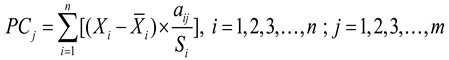
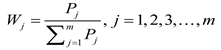 Where PCj represents the score of the j-th principal component. and Si represent the mean and Standard Deviation of the i-th individual indicator, respectively. aij represents the loading of the i-th indicator on the j-th principal component. Wj denotes the weight of the j-th principal component, and Pj denotes the contribution rate of the j-th principal component.
(2) The membership function value for each principal component was calculated as follows:
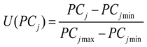 Where U(PCj) represents the membership function value of the j-th principal component, while PCjmin and PCjmax denote the minimum and maximum scores of the j-th principal component, respectively.
(3) The comprehensive evaluation index was then calculated as follows:
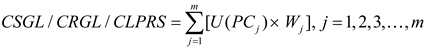 Where CSGL (Comprehensive Shoot Growth Level), CRGL (Comprehensive Root Growth Level), and CLPRS (Comprehensive Level of Physiological Regulatory Substances) denote the composite indices of shoot growth, root growth, and physiological regulatory substances, respectively.
2.4.2. Calculation of the Developmental Stage Index (DVS)
To account for interannual variations in sowing dates and weather, crop developmental stages were normalized using active accumulated temperature (AT). Based on previous studies [28], summer maize reached tasseling at 52 DAS, marking the transition from vegetative to reproductive growth. Accordingly, the growth period was divided into two stages: sowing to tasseling (AT₁) and tasseling to harvest (AT₂). The normalized development stage index (DVS) on day j was calculated as:
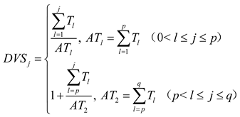 where p denotes the number of days in the first stage, defined as the period from sowing to tasseling in summer maize; q represents the total number of days in the entire growing period; Tₗ is the daily active temperature. When Tₗ ≥ 10 °C, it equals the mean air temperature on the l-th day; otherwise, Tₗ is set to zero. In addition, when 0<j≤p, DVSⱼ ranges from 0.0 to 1.0; when p<j≤q, DVSⱼ ranges from 1.0 to 2.0.
According to Eq. 6, the relationship between the normalized development stage index (DVS) and days after sowing (DAS) during the experimental period was obtained, as shown in Figure 3.
2.5. Determination of the Dynamic Salt Tolerance Coefficient (αSTT) and Quantification of the Salt Tolerance Threshold
2.5.1. Definition of the Dynamic Salt Tolerance Coefficient (αSTT)
To quantify the real-time responsiveness of summer maize to salt stress across different growth stages, a dimensionless parameter, termed the dynamic salt tolerance coefficient (αSTT), was defined in this study. This coefficient characterizes the extent to which plant physiological activity and growth vigor are maintained under saline stress relative to the CK treatment, with values ranging from 0.6 to 1.0. Values of αSTT below 1.0 indicate that plant growth is adversely affected by environmental salt stress, whereas values of αSTT equal to 1.0 indicate that plants have adapted to saline conditions, with the negative effects of salt stress largely mitigated.
2.5.2. Evaluation Criteria Based on Absolute Growth Rate
In the determination of αSTT, the absolute growth rate (AGR) was employed as one of the evaluation criteria in this study. Compared with the relative growth rate (RGR), AGR more accurately represents the absolute magnitude of biomass accumulation per unit time. The calculation of AGR is given as follows:
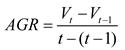 where Vt denotes the observed value at the current time point, Vt-1 denotes the observed value at the previous time point, and t-(t-1) represents the time interval (days) between two consecutive observations.
2.5.3. Assignment Method of the Dynamic Salt Tolerance Coefficient (αSTT)
A hierarchical, nested decision framework was established in this study to determine the dynamic salt tolerance coefficient (αSTT) at each growth stage, based on the coordinated performance of CLPRS, CRGL, and CSGL for each tested treatment relative to the CK treatment. The framework comprises the following six levels: (1) Level 1: If CSGL ≥ 90% of CSGLCK and its absolute growth rate (AGR) ≥ AGRCK, the plant is considered fully adapted to salt stress, and αSTT is set to 1.0. (2) Level 2: If Level 1 is not satisfied, but the AGR of CSGL≥ AGRCK, the plant is considered to have exhibited significant recovery in growth vigor , and αSTT is set to 0.9. (3) Level 3: If Levels 1–2 are not satisfied, but CRGL ≥ 90% of CRGLCK, the root system is considered to have achieved a high level of compensatory growth, and αSTT is set to 0.85. (4) Level 4: If Levels 1–3 are not satisfied, but AGR of CRGL ≥ 90% of AGRCK, the root system is considered to have activated compensatory developmental mechanisms, and αSTT is set to 0.7. (5) Level 5: If Levels 1–4 are not satisfied, but CLPRS ≥ 90% of CLPRSCK, the plant’s physiological regulatory mechanisms are considered activated, and αSTT is set to 0.7. (6) Level 6: If none of the previous levels are satisfied, the plant’s physiological regulatory mechanisms are considered inactive or failed, and αSTT is set to 0.6.
2.5.4. Quantification of the Salt Tolerance Threshold (STT)
(1) Determination of STT for the CK Treatment
To ensure the reliability and objectivity of the evaluation system, the initial STT for each treatment before the FTS was determined according to the STT recommended by the seed company for this maize variety. This value served as the reference point for calculating the STTs of all other treatments.
(2)Determination of Quantitative Formula for STT
To prevent STT from decreasing as maize progresses through its growth stages, a non-decreasing constraint was applied in the calculation of the STT. Specifically, at each developmental stage, STT was determined as the maximum of two candidate values:
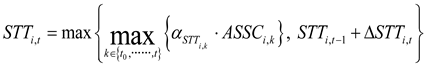
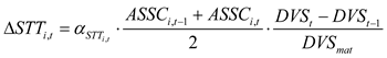 where STTi,t and STTi,t-1 are the STT of treatment i at stage t and t-1, respectively; △STTi,t is the incremental increase of treatment i in the STT from stage t-1 to t; k is the stage variable, representing any growth stage from the initial stage t0 to the current stage t; αSTT i,stage and ASSCi,stage (stage∈[k,t,t-1]) denote the dynamic salt tolerance coefficient and the average soil salt content of rootzone (g/kg) of treatment i at the corresponding stages, respectively; DVSt and DVSt-1 represent the developmental stage index at stage t and t-1, respectively; and DVSmat is the developmental index at crop maturity stage, set to 2.0.
2.6. Framework and Modeling Strategy for Salt Tolerance Threshold Prediction
Accumulating evidence from plant physiology and molecular biology indicates that crops can develop “stress memory” following an initial stress exposure, whereby alterations in physiological and metabolic states are retained, enabling faster and stronger defense responses upon subsequent exposure to the same or more severe stress[20,27]. This suggests that the effect of salinity on the salt tolerance threshold (STT) may not be a purely negative inhibition, but rather a dynamic regulatory process operating across temporal scales. In view of the fact that conventional static mapping approaches often neglect stress memory effects in crops, and thus struggle to address this issue, a unified dynamic predictive framework was developed in this study (Figure 4) to enable dynamic and accurate prediction of STT.
The operational procedure of this framework includes four core steps: Firstly, collect irregular time-series data from multiple sources, encompassing DVS, historical STT estimates, and average soil salt content (ASSC); Secondly, depending on the modeling pathway, represent key information either through feature engineering or by imposing pathway-specific structural constraints on the predictive model; Thirdly, a predictive model is constructed to estimate STT; Fourthly, employ a temporal recursive prediction [31] or reference correction mechanism [32], in which historical observations are prioritized during prediction. In cases of missing observations, the model automatically reuses previous predictions to achieve continuous estimation of the STT throughout the entire growing period.
2.6.1. Modeling Pathways Based on Different Information Representations
Based on this general framework, three specific modeling pathways were designed in this study, which differ in algorithm selection and feature construction but all follow the unified computational procedure described above. The three pathways are detailed as follows:
(1) Pathway I: Recursive Prediction Modeling based on DVS Grids (RP-DG)
Discrete observations were mapped onto a regularized developmental grid defined along the DVS axis, and historical STT states together with corresponding ASSC–DVS information were integrated into a flattened feature representation to support recursive STT prediction. Model training and prediction were implemented using three machine learning algorithms, namely partial least squares regression (PLS), Gaussian process regression (GPR), and CatBoost for comparative evaluation.
(2) Pathway II: Recursive Prediction Modeling based on Dynamic Memory Features (RP-DMF)
The first-order rate of change and the second-order acceleration were computed based on the raw DVS intervals to capture instantaneous response dynamics, while the cumulative integral of ASSC with respect to DVS represented stress memory. These features were combined with ASSC and DVS at the current and two preceding time steps, as well as STT from the two preceding time steps, to form a flattened feature vector. Model training and prediction were conducted using PLS, GPR, and CatBoost for comparative evaluation.
(3) Pathway III: Process-constrained Residual Modeling based on Salt Tolerance Potential (PCR-STP)
Discrete observations were first mapped onto a regularized DVS grid to generate a dense temporal sequence. A baseline STT trajectory was then constructed under the assumption that the salt tolerance potential of unstressed summer maize (CK) follows a logistic-type growth pattern, adopted here as a generic functional form to characterize sigmoidal responses of crop physiological traits to environmental gradients and developmental progression under salinity stress [33]. Residuals between measured STT and the baseline, R(t) = STTobs(t) - STTbase(t), were then modeled using PLS, GPR, and CatBoost to capture stress-induced deviations. The final STT predictions were obtained by summing the logistic baseline with the model-predicted residual corrections.
2.6.2. The Implementation and Configuration of Algorithm
To guarantee prediction robustness across the three modeling pathways, all employed algorithms were uniformly configured.
Across all three modeling pathways, Gaussian process regression (GPR) employed a combination of a radial basis function (RBF) kernel and a white noise kernel as the covariance function K(x, x') [34]:
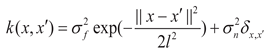 where x and x' are the input feature vectors; σf2 denotes the signal variance, reflecting the overall amplitude of STT fluctuations; l is the characteristic length scale, which governs the smoothness of STT responses to changes in input variables; and σn2 represents the observation noise variance, used to suppress random field fluctuations and enhance model robustness. The kernel hyperparameters were automatically optimized during training using maximum likelihood estimation.
In addition, partial least squares regression (PLS) was employed as a linear baseline model, in which the mapping between input variables and STT was constructed by extracting latent components that maximize their covariance [35]. For consistency across modeling pathways, the number of retained components was fixed at 2. Meanwhile, CatBoost reduces the risk of error accumulation during recursive prediction via Ordered Boosting [36], and its scale-invariant property ensures robust processing of heterogeneous features across all modeling pathways.
2.7. Statistical Analysis
All experimental data were processed using Microsoft Excel 2016 (Microsoft Corp., Redmond, WA, USA). Statistical analyses were conducted with SPSS statistics 25 (SPSS Inc. IBM Corp., Armonk, NY, USA), and graphical outputs were produced using Origin 2021 (OriginLab Corp., Northampton, MA, USA). Mean comparisons among treatments were performed using the Duncan test at a significance level of p < 0.05.
3. Results
3.1. Dynamic Changes in Photosynthetic Characteristics
It has been well established that approximately 90–95% of summer maize biomass is derived from photosynthesis, and grain yield is therefore closely associated with leaf photosynthetic characteristics[37,38]. As shown in Figure 5, leaf net photosynthetic rate (Pn), stomatal conductance (Gs), and transpiration rate (Tr) of summer maize consistently displayed a unimodal pattern over the entire growth period, whereas intercellular CO₂ concentration (Ci) followed a decreasing–increasing–decreasing trajectory. Specifically, pronounced increases in Pn, Gs, and Tr were observed across all treatments during the first training stage (FTS; 21~28 DAS) and the subsequent recovery stage (29~34 DAS). After entering the ten-leaf stage (35 DAS), the magnitude of increase in photosynthetic parameters generally diminished, whereas the rate of increase in Tr under the S1-2-3、S1-3-3、S2-2-3 and S2-3-3 treatments instead accelerated. During the severe stress test stage (SSTS; 52~66 DAS), Pn, Gs, and Tr under all treatments reached their peak values. Among them, The highest Tr was observed under S2-3-3, whereas the highest Pn and Gs occurred in CK. Thereafter, Pn, Gs, and Tr under all treatments began to decline. The rates of decline under S2-2-3 and S2-3-3 were faster than those under the other treatments. In contrast, S0-2-3 and S0-3-3 exhibited a relatively slower decrease in these parameters. At 74 DAS, Pn, Gs, and Tr under S2-2-3 and S2-3-3 had declined to levels lower than those observed in the other treatments. This declining trend was consistently maintained until the end of the grain-filling stage, at which point Pn, Gs, and Tr under all treatments reached their minimum values over the entire growth period.
In contrast, Ci exhibited a trend opposite to that of the other photosynthetic parameters. Prior to tasseling (52 DAS), Ci continuously declined in response to the progressive increase in photosynthetic rate. Upon entering the SSTS, the rate of decline in Ci slowed, and during this stage, Ci under all treatments reached local minimum levels. Subsequently, Ci began to increase under all treatments, with markedly greater increases observed under S2-2-3 and S2-3-3 than under the other treatments. However, after 74 DAS, despite Pn continuing to decline, Ci resumed a declining trend due to leaf senescence. By 86 DAS, Ci under all treatments fell below 100 μmol·mol⁻¹, reaching the minimum levels over the entire growth period. In addition, except for S2-3-3, no significant differences in Ci were observed among the other treatments.
3.2. The Correlations between Different Physiological Regulatory Substances
In this study, Pearson correlation analysis was performed on 14 physiological regulatory indicators at the FTS under three salinity levels (S0, S1, and S2). The analysis revealed that antioxidant enzymes—superoxide dismutase (SOD), peroxidase (POD), and catalase (CAT)—consistently exhibited strong synergistic relationships (Figure 6). Positive correlations among these enzymes were observed across all levels. At S1 level, the pairwise correlations among them were all greater than 0.6. However, enzyme activities were not consistently coordinated with the membrane lipid peroxidation product malondialdehyde (MDA). Specifically, POD and CAT were significantly positively correlated with MDA under S0 level, whereas this association weakened markedly with higher salt-tolerance-training levels. In contrast, the correlation between SOD and MDA was positive under S0 and S2 levels and negative under S1 level, with the absolute values of the correlation coefficients remaining below 0.2 across all levels. Among plant hormones, growth-promoting hormones—including IAA, zeatin, cis-zeatin (CZ), trans-zeatin (TZ), and GA3—were predominantly positively correlated, and the strongest positive correlations were observed under S1 level. In contrast, the stress hormone abscisic acid (ABA) was generally negatively correlated with growth-promoting hormones. For osmotic adjustment substances, positive correlations predominated intrinsically under S0 and S2 levels, whereas negative correlations were predominant under S1 level. Notably, Na⁺ and soluble protein (SP) were significantly positively correlated under all levels.
Based on the correlation analysis described above, a subsequent screening of physiological regulatory indicators was conducted. First, the cumulative number of times that each indicator showed significant correlations (P < 0.05) with other indicators under the three levels was counted. The results showed that POD, CAT, TZ, IAA, and Na⁺ each exhibited ten or more significant correlations with other biochemical indicators, suggesting that these indicators can be identified as key physiological regulatory indicators. Second, supplementary indicators were included based on specific physiological response mechanisms. Although Ca²⁺, SP, and total soluble sugars (TSS) showed relatively fewer overall significant correlations, they are closely linked to the core physiological mechanisms underlying crop responses to salt stress. With respect to SP, it is the only physiological regulatory substance that showed a significant positive correlation with the toxic factor Na⁺ under S0, S1, and S2 levels, and was therefore identified as a key physiological regulatory indicator. With respect to TSS, given that osmotic adjustment is mediated primarily through two major pathways, namely nitrogen metabolism (represented by SP) and carbon metabolism (represented by TSS) [39,40], the inclusion of TSS as a complementary reference indicator is essential for a comprehensive evaluation of metabolic balance. Regarding Ca²⁺, no strong association with Na⁺ was observed under S0 and S1. However, the correlation coefficient between Ca²⁺ and Na⁺ increased markedly under S2 level. This strong association activated under conditions of severe stress and acclimation, provides clear evidence that Ca²⁺ can also serve as a key physiological regulatory indicator.
3.3. Integrated Evaluation of Morphological and Physiological Changes across Developmental Stages
To ensure temporal alignment of indicator measurements and maintain analytical rigor in subsequent statistical analyses, the measurement times of all key physiological regulatory indicators were used as a reference and sequentially numbered, as shown in Table 3.
Based on the data aligned to the reference time numbering (Table 3), principal component analysis (PCA) was conducted separately on key physiological regulatory substances, shoot traits, and root system traits. Principal components with eigenvalues greater than 1 were retained, and the results are presented in Table 4. Specifically, the comprehensive level of physiological regulatory substance (CLPRS) was quantified using eight indicators: POD, CAT, IAA, TZ, Na⁺, soluble protein (SP), total soluble sugar (TSS), and Ca²⁺. The comprehensive shoot growth level (CSGL) was based on six indicators: plant height (H), leaf area index (LAI), shoot biomass (SB), net photosynthetic rate (Pn), transpiration rate (Tr), and stomatal conductance (Gs). The comprehensive root growth level (CRGL) was calculated from 12 indicators: fine root length density (FRLD) at the 0–10, 10–20, 20–30, and 30–40 cm depth intervals; fine root biomass at the 0–10, 10–20, 20–30, and 30–40 cm depth intervals; and fine root surface area at the 0–10, 10–20, 20–30, and 30–40 cm depth intervals.
As shown in Table 4, a total of three, one, and two principal components were extracted for CLPRS, CSGL, and CRGL, respectively, with cumulative contribution rates all exceeding 73%. The results for CSGL indicate that the selected shoot physiological growth indicators of summer maize displayed strong synergistic responses to salt stress, with the first principal component encompassing the majority of the original data’s feature information.
Using the membership function method, the temporal dynamics of each comprehensive indicator for different treatments throughout the entire growth period were quantified, and the results were visualized as shown in Figure 7.
The analysis indicated that CLPRS values during the T2a period were markedly higher than those of the control (CK) in all treatments initially exposed to salt stress at six-leaf stage, among which the S2-2-3 and S2-3-3 treatments showed no significant difference from the CK treatment at the end of the FTS, and during the second training stage (STS), an increase in CLPRS was observed only in S0-2-3 and S0-3-3, which were initially exposed to salt stress.
During the recovery period after the FTS, CRGL increased substantially across all treatments, whereas the rate of increase began to decline during the STS, particularly in treatments that underwent salt stress at the six-leaf stage, where the attenuation in growth increment was consistently lower than that of CK. In contrast, the S0-2-3 and S0-3-3 treatments, which were initially exposed to salt stress at the ten-leaf stage, exhibited a significantly smaller increase during this stage compared with CK, but displayed a pronounced compensatory rebound during the mid-to-late growth stages. Specifically, the compensatory rebound in S0-3-3 occurred during the recovery period after the STS, whereas in S0-2-3, this rebound was delayed until the SSTS.
Overall, following the initial exposure to salt stress, summer maize showed maintenance or enhancement of CLPRS relative to the CK treatment. After a response period, the growth rate of CRGL exhibited either an alleviation of decline or a compensatory rebound relative to CK.
3.4. Quantification of Salt Tolerance Threshold across Developmental Stages
The variations in the average soil salt content (ASSC) within the 0–40 cm rootzone soil under different regimes of brackish water irrigation throughout the growth period are shown in Figure 8. Using the salt tolerance threshold (STT) quantification method outlined in Section 2.5, the STT for summer maize at various growth stages was determined. The results for the dynamic salt tolerance coefficient (αSTT) and STT are presented in Table 5 and Table 6, respectively.
As shown in Table 5, the dynamic salt tolerance coefficient (αSTT) of summer maize demonstrates significant regulatory characteristics throughout the growth stages. For the S0-2-3 and S0-3-3 treatments, which were not subjected to salt stress training at the six-leaf stage, the αSTT remained at 1.0 (no stress level) until 35 DAS. However, after they were subjected to salt stress for the initial time during the STS, the αSTT declined rapidly to approximately 0.7. In contrast, S1-2-3, S1-3-3, S2-2-3, and S2-3-3 underwent their initial salt-tolerance training at the six-leaf stage. Despite relatively low αSTT (0.6–0.7) at 28 DAS, they gradually increased as the growth stages progressed. During the process, the second training at the ten-leaf stage did not result in a decline in their αSTT. After the STS, the αSTT of all treatments maintained an upward trend. However, during the SSTS, the αSTT of S2-2-3 and S2-3-3 decreased from 1.0 to 0.85, whereas the αSTT of S1-3-3 remained constant. The other treatments showed varying degrees of increase, with S1-2-3 reaching an αSTT of 1.0 at 66 DAS, indicating full adaptation to the salt stress conditions by this stage.
As shown in Table 6, from 0 to 21 DAS, the STT for all treatments was set at the seed company’s recommended value of 1.3 g/kg. Following the FTS, STT began to change across treatments, but the differences remained minor until the end of the STS (45 DAS). At 45 DAS, treatments that experienced salt-stress-training during the six-leaf stage showed marked increases in STT, all exceeding 1.8 g/kg, with the S2-3-3 treatment attaining the maximum value of 2.33 g/kg. By comparison, S0-2-3 and S0-3-3, which had just completed their initial exposure to salt stress at this stage, showed STT similar to CK at approximately 1.5 g/kg. Thereafter, STT continued to increase at differing rates across treatments, with all experimental treatments surpassing CK in the magnitude of increase, while S0-2-3 and S0-3-3 consistently showed lower STT compared with the other experimental treatments. At 66 DAS, CK exhibited an STT of 1.7 g/kg, considerably lower than the other treatments, whereas S0-2-3 and S0-3-3 had STT values below 3 g/kg, still lower than the other experimental treatments. The highest STT, 3.35 g/kg, was recorded for S1-2-3 and S2-3-3, with S1-2-3 representing the only experimental treatment at this stage whose STT matched the extrinsic rootzone environment.
3.5. The Predictive Performance of STT using Different Modeling Pathways
The formation of STT is closely associated with crop growth states under stress, which are jointly driven by developmental progression and environmental conditions [25,41]. Given that soil salinity represents a key environmental factor and that soil salt content can be continuously quantified to characterize environmental variability in this study, soil salt content (ASSC) was adopted as the primary environmental descriptor. Accordingly, a prediction scheme was constructed using DVS and ASSC as input variables and STT as the output variable.
Based on the three modeling pathways and three machine learning algorithms described in Section 2.6, leave-one-out validation (LOOCV) was employed to evaluate predictive performance. The relationship between predicted and measured STT values is illustrated in Figure 9. Model performance was evaluated using the coefficient of determination (R²) and the root mean square error (RMSE).
As shown in Figure 9, the PCR-STP pathway achieved better predictive performance, with leave-one-out validation (LOOCV) R² values of 0.880, 0.843, and 0.910 for PLS, GPR, and CatBoost, respectively, consistently outperforming the RP-DG and RP-DM pathway. Among the three algorithms, CatBoost consistently exhibited the best performance, with kernel density plots across all pathways showing high-density distributions with peak densities near the upper color-scale limit, and R² and RMSE values superior to those of PLS and GPR within each pathway. By contrast, GPR outperformed PLS only under the RP-DMF pathway, whereas its predictive performance was inferior to that of PLS under the RP-DG and RP-DMF pathways.
4. Discussion
4.1. Two-Stage Physiological Regulatory Responses of Summer Maize to Salinity Stress
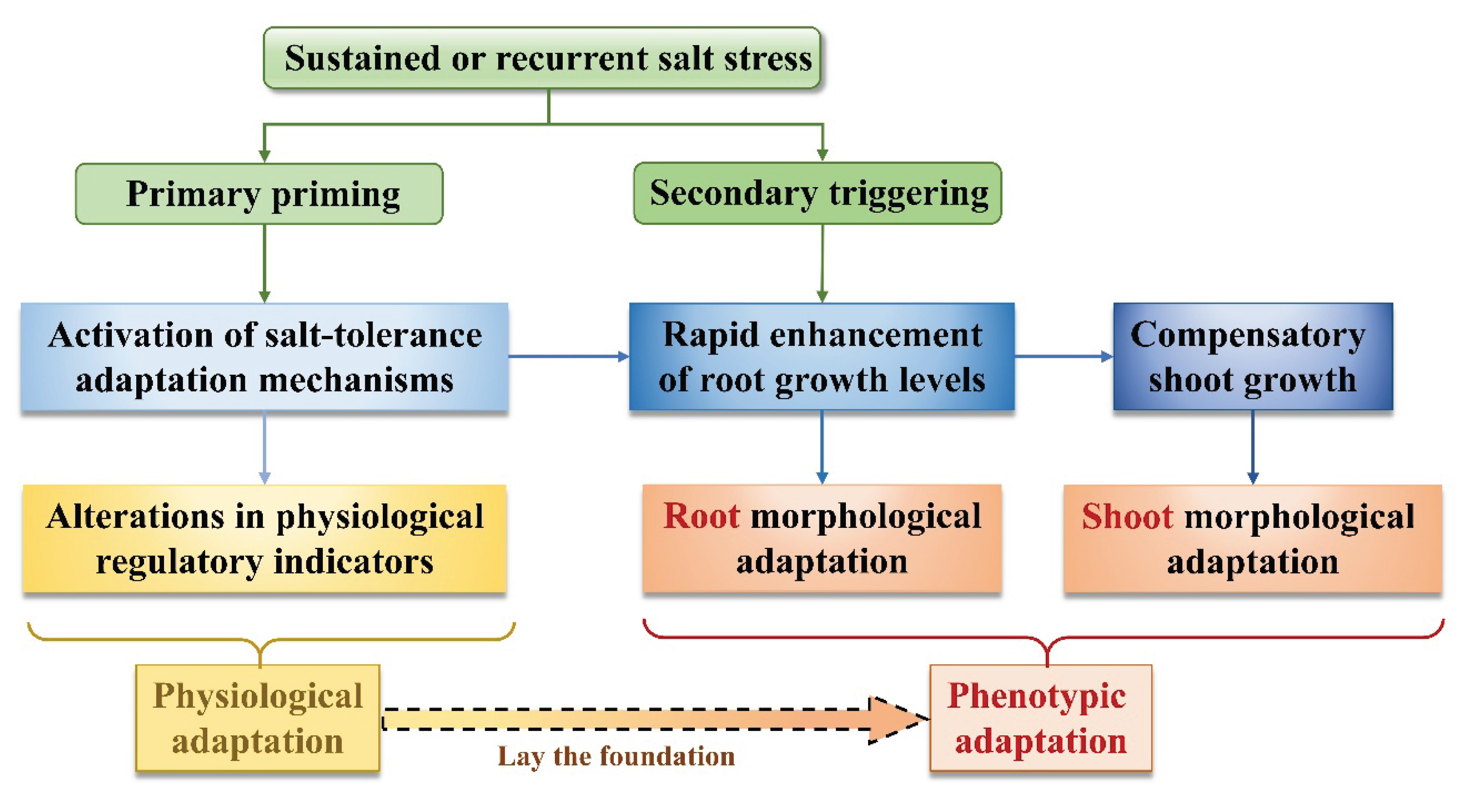
Numerous studies have demonstrated that plant adaptation to salt stress, referred to as salt tolerance, is a complex outcome resulting from the combined effects of genetics, variation, and environmental factors, which is manifested by changes in physiological phenotypic traits and intrinsic biochemical levels [16,42,43]. This study found that the stress-resistance response of summer maize to salt stress exhibits a clear two-stage characteristic, namely that physiological adaptation is initiated first, followed by phenotypic adaptation, with the two jointly forming a complete stress-resistance system.
Specifically, although different training modes induced varying salt stress memory effects, the initial exposure to salt stress consistently triggered a regulated CLPRS response in summer maize, characterized by maintenance or enhancement relative to the CK treatment, regardless of the stress intensity. This inducible physiological state was closely associated with the coordinated responses of key regulatory mechanisms, including enhanced antioxidant enzyme activities, dynamic modulation of growth-related hormones, and the accumulation of osmotic adjustment substances. This interpretation is consistent with the findings of Zhu [44], who reported that early-stage physiological regulation plays a decisive role in enabling rapid crop adaptation to salt stress. With the prolongation of salt stress and the progression of developmental stages, the regulatory emphasis in summer maize progressively shifted from intrinsic biochemical adjustments to physiological and phenotypic traits, representing the second stage of the adaptive response. The results indicate that following the rapid response of CLPRS, comprehensive root growth level (CRGL) exhibited discernible adjustments, characterized by an alleviation of growth-rate decline or a compensatory increase relative to CK, suggesting that microscopic physiological regulation can induce a rapid improvement in root growth distribution levels , thereby facilitating adaptation to or mitigation of salt stress effects. In the study by Wang et al. [45], salt stress enhanced auxin transport activity, thereby promoting lateral root growth and development and improving crop salt tolerance, which corroborates the changes in CRGL observed in this study, indicating that root morphological adjustment is a core pathway of phenotypic adaptation to salt stress.
From another perspective, different training modes of salt stress priming markedly affected both the onset timing and the degree of coordination between the two adaptive response stages. For treatments receiving salt-stress training at the six-leaf stage, physiological adaptive mechanisms were triggered earlier, and, with the exception of S1-3-3, root systems exhibited pronounced compensatory growth following the second training stage, resulting in sustained high CRGL levels from tasseling through silking (52~66 DAS), among which S1-2-3 exhibited CSGL most comparable to those of the CK across the six experimental treatments. In contrast, when salt-stress-training was initially imposed at the ten-leaf stage, physiological adaptive responses were also rapidly initiated; however, the responses of root development, shoot growth, and photosynthetic activity exhibited noticeable delays. These differences suggest that salt-stress training does not simply enhance or suppress a single indicator, but rather reshapes the overall stress-resistance strategy of crops by altering the relationship between physiological regulation and growth responses.
Figure 10.
The priming process of summer maize salt tolerance under salt-tolerance training.
4.2. Dynamic Variation of Salt Tolerance in Summer Maize Under Different Training Modes of Salt Stress Priming
In light of the two-stage stress-regulation response characteristics identified in Section 4.1, crop salt tolerance should be understood not as a static trait, but as a dynamic property that evolves in response to developmental progression and environmental conditions, consistent with findings reported in previous studies [46,47]. To better characterize the dynamic nature of salt tolerance, a stage-specific evaluation framework incorporating CSGL, CRGL, and CLPRS was developed. This framework allowed the derivation of a dynamic salt tolerance coefficient (αSTT) for summer maize at different growth stages, thereby providing a quantitative basis for characterizing the salt tolerance threshold (STT) across these stages.
The results of αSTT clearly revealed differences in the regulation of salt tolerance among the training modes of salt stress priming. In all experimental treatments, αSTT sharply declined following the initial exposure to salt stress, reflecting the commonly observed temporary growth suppression during the initial phase of salinity stress [48,49]. Thereafter, αSTT gradually recovered as the growth period progressed and physiological adaptive mechanisms were activated, yet significant differences were observed among different salt-stress-training treatments. In the S2-2-3 and S2-3-3 treatments, αSTT reached 1.0 upon entering the tasseling stage (52 DAS) but declined in later stages, demonstrating that salt tolerance does not simply accumulate over prolonged stress. Munns and Tester [50] demonstrated that prolonged stress increases metabolic burden and overutilizes regulatory resources, which likely accounts for the decline in αSTT observed in S2-2-3 and S2-3-3. In contrast, αSTT in S1-2-3 steadily increased after the first training stage (FTS) and reached 1.0 during the late growth stages, suggesting that this treatment induced a stable and sustained salt tolerant state in summer maize. Previous studies have found that when the intensity and timing of salt stress are within a suitable range, the resulting physiological adjustments can effectively enhance crop salt tolerance in subsequent growth stages without markedly suppressing growth [51,52,53]. The performance of S1-2-3 aligns well with this finding, indicating that the timing and intensity of salt-stress training are critical for establishing effective salt tolerance.
It should be noted that in this study, the dynamic changes of the STT did not fully correspond with those of αSTT. For example, in S0-2-3 and S0-3-3, αSTT reached 0.9 at 66 DAS, which was comparable to S1-3-3 and higher than S2-2-3 and S2-3-3; however, their STT remained lower than that of the other experimental treatments, which may be attributed to the absence of salt stress priming during the early growth stage, leading to relatively low rootzone salinity and thus constraining the increase in STT. This indicates that αSTT primarily represents the crop's intrinsic regulatory potential for salt tolerance at a given growth stage, whereas STT reflects the effective expression of this potential under actual saline conditions. Prior research indicates that crop physiological responses to salinity are modulated by stress intensity, duration, and growth stage, and that the specific characteristics and magnitude of these responses may vary considerably with environmental conditions [46,49,54]. Therefore, evaluations of salt tolerance need to consider the actual salinity environment for comprehensive analysis; otherwise, it is difficult to accurately reflect the true salt tolerance of crops under salt stress conditions. This provides further support for the distinction between αSTT and STT identified in this study. Moreover, in S1-2-3, extrinsic rootzone environment reached a relatively optimal range during late development and αSTT reached 1.0, resulting in higher STT. This demonstrates that under an appropriate salt-stress-training mode, the crop's regulatory potential for salt tolerance can steadily improve and effectively translate into tolerance to higher salinity levels. This result further confirms the importance of training modes of salt stress priming with appropriately matched timing and intensity in enhancing crop salt tolerance.
4.3. Quantification of Salt Stress Memory Effects and Dynamic Prediction of the Salt Tolerance Threshold
Following the elucidation of dynamic patterns of salt tolerance in summer maize under different training modes of salt stress priming, further investigation into effective prediction of this dynamic process is essential for enhancing the practical applicability of quantitative STT assessments. To address the dynamic issue arising from the variation of STT with crop developmental progression, a unified framework for STT prediction was established in this study, within which three distinct modeling pathways were designed, and on this basis, the performance of three machine learning algorithms in predicting STT was systematically evaluated.The results showed that the PCR-STP pathway combined with CatBoost achieved the highest prediction accuracy, as evidenced by LOOCV R² of 0.910 and RMSE of 0.241. In addition, under the PCR-STP pathway, the prediction performance of all algorithms was superior to that of the other pathways. This may be attributed to the fact that the PCR-STP pathway does not solely rely on feature transformations to represent temporal information , but instead incorporates physiologically meaningful process constraints to treat the dynamic variation of STT over the growth process in an integrated manner, thereby constraining unreasonable prediction fluctuations and making model outputs more consistent with actual variation patterns. In recent years, growing attention has been paid to incorporating multi-level process information or physiological assumptions into data-driven models when addressing bio–environmental dynamic systems characterized by clear stage dependency or process constraints, with the aim of enhancing the stability and consistency of predictions [55,56]. Related studies have indicated that, despite their strong nonlinear fitting capacity, purely data-driven models may suffer from reduced predictive stability in systems governed by explicit process constraints or stage-dependent dynamics, owing to excessive model flexibility [57]. By contrast, embedding appropriate process constraints within model architectures helps improve both predictive accuracy and generalization. For instance, Liu et al. [58] mbedded process-based model knowledge into a machine learning framework, thereby achieving performance that was markedly superior to that of purely data-driven approaches in dynamic prediction of complex ecosystems. These findings provide theoretical support for the superior predictive performance of the PCR-STP pathway observed in the present study.
In terms of algorithmic performance, CatBoost consistently outperformed PLS and GPR across all modeling pathways, demonstrating its stronger predictive capability within the unified STT prediction framework proposed in this study. Notably, relative to the purely data-driven RP-DG and RP-DMF pathways, the differences in prediction accuracy among the three algorithms were reduced under the PCR-STP pathway. This finding suggests that once the modeling pathway reasonably accounts for the dynamic nature of STT, prediction outcomes become less sensitive to algorithm selection, leading to a convergence in predictive performance across different algorithms.
Overall, in contrast to previous salt tolerance prediction studies that focus on algorithmic performance comparisons, this study systematically analyzed the interaction between modeling pathways and algorithm selection within a unified predictive framework. The results demonstrate that the choice of modeling pathway plays a more important role in STT prediction, whereas algorithm selection functions more as a means of performance optimization.
5. Conclusions
Our study indicates that different training modes of salt stress priming induce distinct stress memory effects in summer maize, which markedly influence the dynamic variation of the salt tolerance threshold (STT), and that maize salt tolerance response mechanisms exhibit distinct stage-specific characteristics throughout the growth period. Principal component analysis (PCA) combined with membership function methods was employed to quantify CSGL, CRGL, and CLPRS across maize growth stages. Integrated evaluation revealed that maize initially undergoes a physiological adaptation phase dominated by intrinsic regulatory adjustments upon first training stage (FTS), which subsequently transitions into a phenotypic adaptation phase marked by enhanced growth performance. The observed differences among training modes indicate that appropriate training mode of salt stress priming (S1-S2-S3) fosters a sustained increase in the dynamic salt tolerance coefficient (αSTT), enabling it to reach 1.0 in the later growth stages and thereby yielding higher STT under elevated rootzone salinity. Conversely, improper salt stress training modes produce adverse effects that hinder STT enhancement. Furthermore, a unified predictive framework for STT was developed, within which the interactions of three distinct modeling pathways and three machine learning algorithms were systematically evaluated. The results indicate that, under the unified predictive framework, the combination of the PCR-STP pathway incorporating process-based constraints and the CatBoost algorithm achieved the highest predictive accuracy. Meanwhile, under this pathway, PLS, GPR, and CatBoost all outperformed the purely data-driven RP-DG and RP-DMF pathways, and the differences among algorithms were reduced. These findings highlight that, for STT, which exhibits distinct stage-dependent dynamics, the rational design of the modeling pathway exerts a more pivotal influence on predictive performance than algorithm selection.
Author Contributions
Conceptualization, S.P. and T.M.; methodology, S.P. and T.M; software, S.P. and Z.Z.; fieldwork, S.P. and T.M; formal analysis, Z.Z. and H.W.; data curation, Q.J and W.S.F.; writing—original draft preparation, S.P. and T.M.; writing—review and editing, S.P., T.M. and J.L.; supervision, T.M. and W.X.; project administration, T.M., J.L. and W.X. All authors have read and agreed to the published version of the manuscript.
Funding
This research was funded by the Key Laboratory of Saline-alkali Soil Improvement and Utilization (Saline-alkali land in arid and semi-arid regions), Ministry of Agriculture and Rural Affairs, P. R. China - Open Fund Project, Project number YJDKFJJ202301 and the National Natural Science Foundation of China (NSFC), grant number 52109051.
Institutional Review Board Statement
Not applicable.
Data Availability Statement
Data is contained within the article.
Acknowledgments
The authors would like to thank Teng Ma, Guangquan Zeng, Dai Yan, Yiqun Yin, Pingru He, Kaiwen Chen and Qiong Wang for their help in the micro-plot experiment.
Conflicts of Interest
The authors declare no conflict of interest.
References
- Sultan, M.T.; Mahmud, U.; Khan, M.Z. Addressing soil salinity for sustainable agriculture and food security: Innovations and challenges in coastal regions of Bangladesh. 2023, 8, 100260. [Google Scholar] [CrossRef]
- Boretti, A.; Rosa, L. Reassessing the projections of the world water development report. NPJ Clean Water 2019, 2, 15. [Google Scholar] [CrossRef]
- Minhas, P.; Ramos, T.B.; Ben-Gal, A.; Pereira, L.S. Coping with salinity in irrigated agriculture: Crop evapotranspiration and water management issues. Agricultural Water Management 2020, 227, 105832. [Google Scholar] [CrossRef]
- Bouksila, F.; Bahri, A.; Berndtsson, R.; Persson, M.; Rozema, J.; Van der Zee, S.E. Assessment of soil salinization risks under irrigation with brackish water in semiarid Tunisia. Environmental and experimental botany 2013, 92, 176–185. [Google Scholar] [CrossRef]
- Zhang, Q.; Qian, H.; Ren, W.; Xu, P.; Li, W.; Yang, Q.; Shang, J. Salinization of shallow groundwater in the Jiaokou Irrigation District and associated secondary environmental challenges. Science of the Total Environment 2024, 908, 168445. [Google Scholar] [CrossRef]
- Munns, R. Comparative physiology of salt and water stress. Plant, cell & environment 2002, 25, 239–250. [Google Scholar]
- Ma, T.; Chen, K.; He, P.; Dai, Y.; Yin, Y.; Peng, S.; Ding, J.; Yu, S.e.; Huang, J. Sunflower photosynthetic characteristics, nitrogen uptake, and nitrogen use efficiency under different soil salinity and nitrogen applications. Water 2022, 14, 982. [Google Scholar] [CrossRef]
- Galić, V.; Mazur, M.; Šimić, D.; Zdunić, Z.; Franić, M. Plant biomass in salt-stressed young maize plants can be modelled with photosynthetic performance. Photosynthetica 2020, 58, 194–204. [Google Scholar] [CrossRef]
- Abdelraheem, A.; Esmaeili, N.; O’Connell, M.; Zhang, J. Progress and perspective on drought and salt stress tolerance in cotton. Industrial Crops and Products 2019, 130, 118–129. [Google Scholar] [CrossRef]
- Moud, A.M.; Maghsoudi, K. Salt stress effects on respiration and growth of germinated seeds of different wheat (Triticum aestivum L.) cultivars. World J. Agric. Sci 2008, 4, 351–358. [Google Scholar]
- Praxedes, S.; De Lacerda, C.; DaMatta, F.; Prisco, J.; Gomes-Filho, E. Salt tolerance is associated with differences in ion accumulation, biomass allocation and photosynthesis in cowpea cultivars. Journal of Agronomy and Crop Science 2010, 196, 193–204. [Google Scholar] [CrossRef]
- Ma, T.; Zeng, W.; Li, Q.; Yang, X.; Wu, J.; Huang, J. Shoot and root biomass allocation of sunflower varying with soil salinity and nitrogen applications. Agronomy Journal 2017, 109, 2545–2555. [Google Scholar] [CrossRef]
- Ma, T.; Zeng, W.; Lei, G.; Wu, J.; Huang, J. Predicting the rooting depth, dynamic root distribution and the yield of sunflower under different soil salinity and nitrogen applications. Industrial Crops and Products 2021, 170, 113749. [Google Scholar] [CrossRef]
- Koevoets, I.T.; Venema, J.H.; Elzenga, J.T.M.; Testerink, C. Roots withstanding their environment: exploiting root system architecture responses to abiotic stress to improve crop tolerance. Frontiers in plant science 2016, 7, 1335. [Google Scholar] [CrossRef]
- Deinlein, U.; Stephan, A.B.; Horie, T.; Luo, W.; Xu, G.; Schroeder, J.I. Plant salt-tolerance mechanisms. Trends in plant science 2014, 19, 371–379. [Google Scholar] [CrossRef] [PubMed]
- Van Zelm, E.; Zhang, Y.; Testerink, C. Salt tolerance mechanisms of plants. Annual review of plant biology 2020, 71, 403–433. [Google Scholar] [CrossRef] [PubMed]
- Mozgova, I.; Mikulski, P.; Pecinka, A.; Farrona, S. Epigenetic mechanisms of abiotic stress response and memory in plants. Epigenetics in plants of agronomic importance: Fundamentals and applications: Transcriptional regulation and chromatin remodelling in plants 2019, 1–64. [Google Scholar]
- Mansour, E.; Moustafa, E.S.; Desoky, E.-S.M.; Ali, M.M.; Yasin, M.A.; Attia, A.; Alsuhaibani, N.; Tahir, M.U.; El-Hendawy, S. Multidimensional evaluation for detecting salt tolerance of bread wheat genotypes under actual saline field growing conditions. Plants 2020, 9, 1324. [Google Scholar] [CrossRef]
- Huqe, M.A.S.; Haque, M.S.; Sagar, A.; Uddin, M.N.; Hossain, M.A.; Hossain, A.Z.; Rahman, M.M.; Wang, X.; Al-Ashkar, I.; Ueda, A. Characterization of maize hybrids (Zea mays L.) for detecting salt tolerance based on morpho-physiological characteristics, ion accumulation and genetic variability at early vegetative stage. Plants 2021, 10, 2549. [Google Scholar] [CrossRef]
- Hilker, M.; Schmülling, T. Stress priming, memory, and signalling in plants. 2019, 42, 753–761. [Google Scholar] [CrossRef]
- Zamani, E.; Bakhtari, B.; Razi, H.; Hildebrand, D.; Moghadam, A.; Alemzadeh, A. Comparative morphological, physiological, and biochemical traits in sensitive and tolerant maize genotypes in response to salinity and pb stress. Scientific Reports 2024, 14, 31036. [Google Scholar] [CrossRef]
- Tian, H.; Liu, H.; Zhang, D.; Hu, M.; Zhang, F.; Ding, S.; Yang, K. Screening of salt tolerance of maize (Zea mays L.) lines using membership function value and GGE biplot analysis. PeerJ 2024, 12, e16838. [Google Scholar] [CrossRef] [PubMed]
- Hassanli, M.; Ebrahimian, H.; Mohammadi, E.; Rahimi, A.; Shokouhi, A. Simulating maize yields when irrigating with saline water, using the AquaCrop, SALTMED, and SWAP models. Agricultural water management 2016, 176, 91–99. [Google Scholar] [CrossRef]
- Caro, M.; Cruz, V.; Cuartero, J.; Estan, M.; Bolarin, M. Salinity tolerance of normal-fruited and cherry tomato cultivars. Plant and soil 1991, 136, 249–255. [Google Scholar] [CrossRef]
- Maas, E.V.; Hoffman, G.J. Crop salt tolerance—current assessment. Journal of the irrigation and drainage division 1977, 103, 115–134. [Google Scholar] [CrossRef]
- Arif, Y.; Singh, P.; Siddiqui, H.; Bajguz, A.; Hayat, S. Salinity induced physiological and biochemical changes in plants: An omic approach towards salt stress tolerance. Plant Physiology and Biochemistry 2020, 156, 64–77. [Google Scholar] [CrossRef]
- Wang, X.; Ge, J.; He, M.; Li, Q.; Cai, J.; Zhou, Q.; Zhong, Y.; Wollenweber, B.; Jiang, D. Enhancing crop resilience: Understanding the role of drought priming in wheat stress response. Field Crops Research 2023, 302, 109083. [Google Scholar] [CrossRef]
- Peng, S.; Ma, T.; Ma, T.; Chen, K.; Dai, Y.; Ding, J.; He, P.; Yu, S.e. Effects of Salt Tolerance Training on Multidimensional Root Distribution and Root-Shoot Characteristics of Summer Maize under Brackish Water Irrigation. Plants 2023, 12, 3329. [Google Scholar] [CrossRef]
- Rosolem, C.A.; Pace, L.; Crusciol, C.A. Nitrogen management in maize cover crop rotations. Plant and Soil 2004, 264, 261–271. [Google Scholar] [CrossRef]
- Ismayilov, A.I.; Mamedov, A.I.; Fujimaki, H.; Tsunekawa, A.; Levy, G.J. Soil salinity type effects on the relationship between the electrical conductivity and salt content for 1: 5 soil-to-water extract. Sustainability 2021, 13, 3395. [Google Scholar] [CrossRef]
- Box, G.E.; Jenkins, G.M.; Reinsel, G.C.; Ljung, G.M. Time series analysis: forecasting and control; John Wiley & Sons, 2015. [Google Scholar]
- Kalman, R.E. A new approach to linear filtering and prediction problems. 1960, 35–45. [Google Scholar] [CrossRef]
- Radanielson, A.M.; Angeles, O.; Li, T.; Ismail, A.M.; Gaydon, D.S. Describing the physiological responses of different rice genotypes to salt stress using sigmoid and piecewise linear functions. Field Crops Research 2018, 220, 46–56. [Google Scholar] [CrossRef] [PubMed]
- Seeger, M. Gaussian processes for machine learning. International journal of neural systems 2004, 14, 69–106. [Google Scholar] [CrossRef]
- Wold, S.; Sjöström, M.; Eriksson, L. PLS-regression: a basic tool of chemometrics. Chemometrics and intelligent laboratory systems 2001, 58, 109–130. [Google Scholar] [CrossRef]
- Prokhorenkova, L.; Gusev, G.; Vorobev, A.; Dorogush, A.V.; Gulin, A. CatBoost: unbiased boosting with categorical features. Advances in neural information processing systems 2018, 31. [Google Scholar]
- Zheng, H.; Wang, J.; Cui, Y.; Guan, Z.; Yang, L.; Tang, Q.; Sun, Y.; Yang, H.; Wen, X.; Mei, N. Effects of row spacing and planting pattern on photosynthesis, chlorophyll fluorescence, and related enzyme activities of maize ear leaf in maize–soybean intercropping. Agronomy 2022, 12, 2503. [Google Scholar] [CrossRef]
- Tollenaar, M.; Lee, E. Dissection of physiological processes underlying grain yield in maize by examining genetic improvement and heterosis. Maydica 2006, 51, 399. [Google Scholar]
- Ashraf, M.; Harris, P.J. Potential biochemical indicators of salinity tolerance in plants. Plant science 2004, 166, 3–16. [Google Scholar] [CrossRef]
- Parida, A.K.; Das, A.B. Salt tolerance and salinity effects on plants: a review. Ecotoxicology and environmental safety 2005, 60, 324–349. [Google Scholar] [CrossRef]
- Shannon, M.; Grieve, C. Tolerance of vegetable crops to salinity. Scientia horticulturae 1998, 78, 5–38. [Google Scholar] [CrossRef]
- Zhou, Y.; Feng, C.; Wang, Y.; Yun, C.; Zou, X.; Cheng, N.; Zhang, W.; Jing, Y.; Li, H. Understanding of plant salt tolerance mechanisms and application to molecular breeding. International Journal of Molecular Sciences 2024, 25, 10940. [Google Scholar] [CrossRef] [PubMed]
- Arzani, A.; Ashraf, M. Smart engineering of genetic resources for enhanced salinity tolerance in crop plants. Critical Reviews in Plant Sciences 2016, 35, 146–189. [Google Scholar] [CrossRef]
- Zhu, J.-K. Abiotic stress signaling and responses in plants. Cell 2016, 167, 313–324. [Google Scholar] [CrossRef]
- Wang, Y.; Li, K.; Li, X. Auxin redistribution modulates plastic development of root system architecture under salt stress in Arabidopsis thaliana. Journal of plant physiology 2009, 166, 1637–1645. [Google Scholar] [CrossRef]
- Negrão, S.; Schmöckel, S.M.; Tester, M. Evaluating physiological responses of plants to salinity stress. Annals of botany 2017, 119, 1–11. [Google Scholar] [CrossRef]
- Liu, C.; Jiang, X.; Yuan, Z. Plant responses and adaptations to salt stress: a review. Horticulturae 2024, 10, 1221. [Google Scholar] [CrossRef]
- Balasubramaniam, T.; Shen, G.; Esmaeili, N.; Zhang, H. Plants’ response mechanisms to salinity stress. Plants 2023, 12, 2253. [Google Scholar] [CrossRef]
- Atta, K.; Mondal, S.; Gorai, S.; Singh, A.P.; Kumari, A.; Ghosh, T.; Roy, A.; Hembram, S.; Gaikwad, D.J.; Mondal, S. Impacts of salinity stress on crop plants: improving salt tolerance through genetic and molecular dissection. Frontiers in Plant Science 2023, 14, 1241736. [Google Scholar] [CrossRef]
- Munns, R.; Tester, M. Mechanisms of salinity tolerance. Annu. Rev. Plant Biol. 2008, 59, 651–681. [Google Scholar] [CrossRef]
- Zhu, Z.; Dai, Y.; Yu, G.; Zhang, X.; Chen, Q.; Kou, X.; Mehareb, E.M.; Raza, G.; Zhang, B.; Wang, B. Dynamic physiological and transcriptomic changes reveal memory effects of salt stress in maize. BMC genomics 2023, 24, 726. [Google Scholar] [CrossRef]
- Alzahrani, O.; Abouseadaa, H.; Abdelmoneim, T.K.; Alshehri, M.A.; El-Mogy, M.; El-Beltagi, H.S.; Atia, M.A. Agronomical, physiological and molecular evaluation reveals superior salt-tolerance in bread wheat through salt-induced priming approach. Notulae Botanicae Horti Agrobotanici Cluj-Napoca 2021, 49, 12310–12310. [Google Scholar] [CrossRef]
- Li, J.; Chen, J.; Jin, J.; Wang, S.; Du, B. Effects of irrigation water salinity on maize (Zea may L.) emergence, growth, yield, quality, and soil salt. Water 2019, 11, 2095. [Google Scholar] [CrossRef]
- Ma, T.; Zeng, W.; Li, Q.; Wu, J.; Huang, J. Effects of water, salt and nitrogen stress on sunflower (Helianthus annuus L.) at different growth stages. Journal of soil science and plant nutrition 2016, 16, 1024–1037. [Google Scholar] [CrossRef]
- Maestrini, B.; Mimić, G.; van Oort, P.A.; Jindo, K.; Brdar, S.; Athanasiadis, I.N.; van Evert, F.K. Mixing process-based and data-driven approaches in yield prediction. European Journal of Agronomy 2022, 139, 126569. [Google Scholar] [CrossRef]
- Shi, Y.; Han, L.; Zhang, X.; Sobeih, T.; Gaiser, T.; Thuy, N.H.; Behrend, D.; Srivastava, A.K.; Halder, K.; Ewert, F. Deep Learning Meets Process-Based Models: A Hybrid Approach to Agricultural Challenges. arXiv preprint arXiv:2504.16141 2025, arXiv:2504.16141. [Google Scholar] [CrossRef]
- Shahhosseini, M.; Hu, G.; Huber, I.; Archontoulis, S.V. Coupling machine learning and crop modeling improves crop yield prediction in the US Corn Belt. Scientific reports 2021, 11, 1606. [Google Scholar] [CrossRef]
- Liu, L.; Zhou, W.; Guan, K.; Peng, B.; Xu, S.; Tang, J.; Zhu, Q.; Till, J.; Jia, X.; Jiang, C. Knowledge-guided machine learning can improve carbon cycle quantification in agroecosystems. Nature communications 2024, 15, 357. [Google Scholar] [CrossRef]
Figure 1.
Variation in precipitation, radiation and temperature.
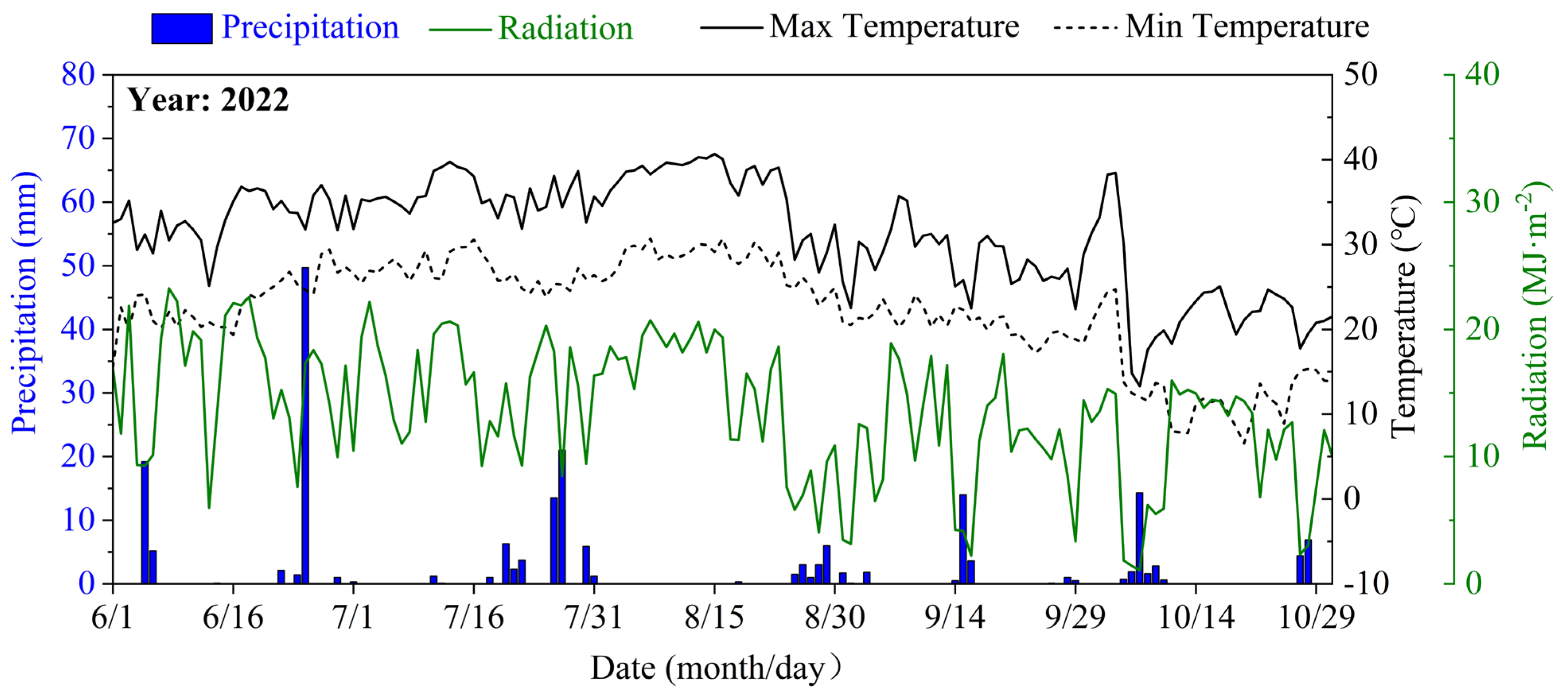
Figure 2.
Schematic representation of the experimental layout, brackish water irrigation design, and multi-dimensional data collection workflows for summer maize.
Figure 2.
Schematic representation of the experimental layout, brackish water irrigation design, and multi-dimensional data collection workflows for summer maize.
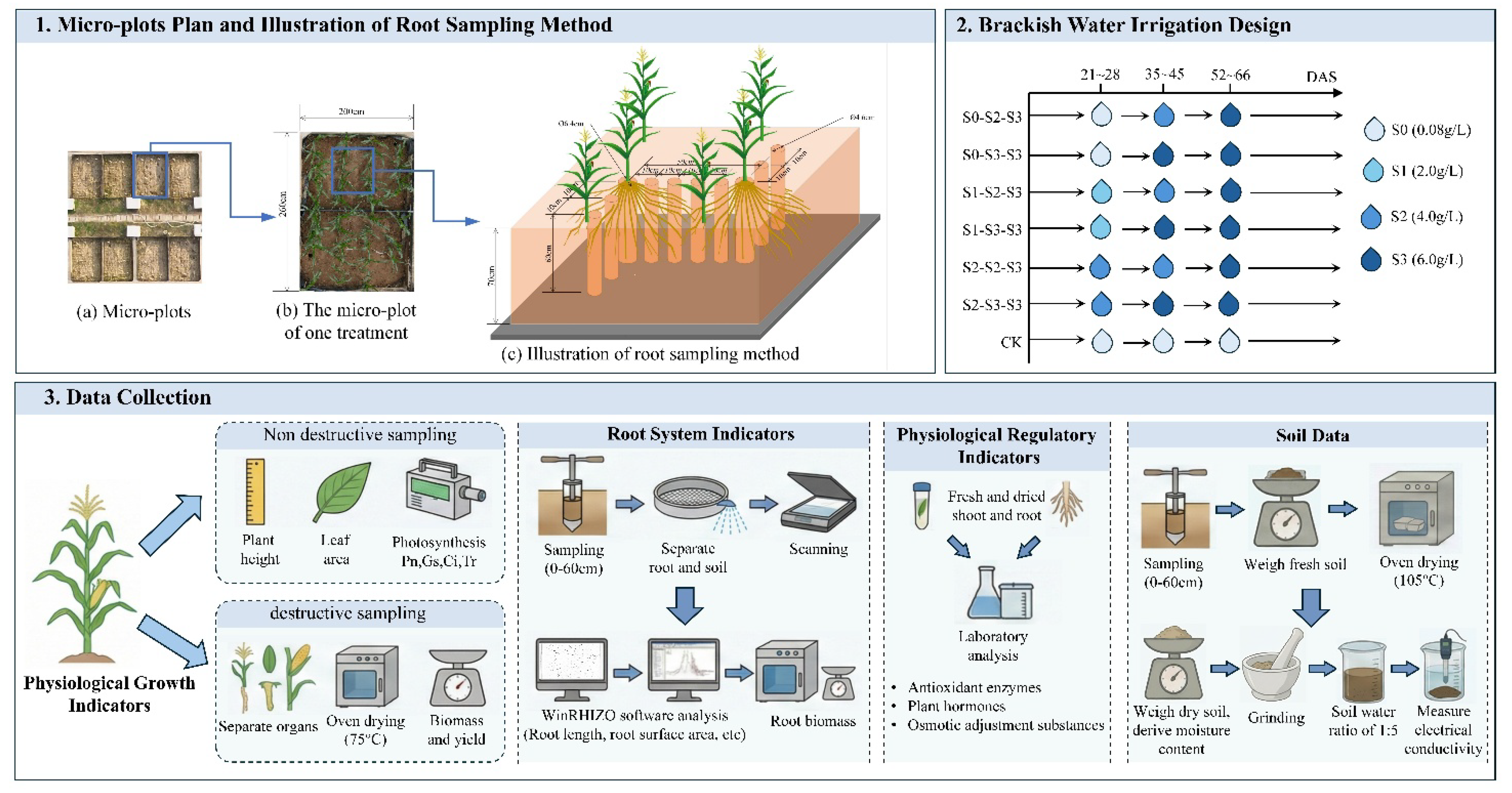
Figure 3.
Scatter plot of normalized developmental stage index (DVS) versus days after sowing (DAS).
Figure 3.
Scatter plot of normalized developmental stage index (DVS) versus days after sowing (DAS).
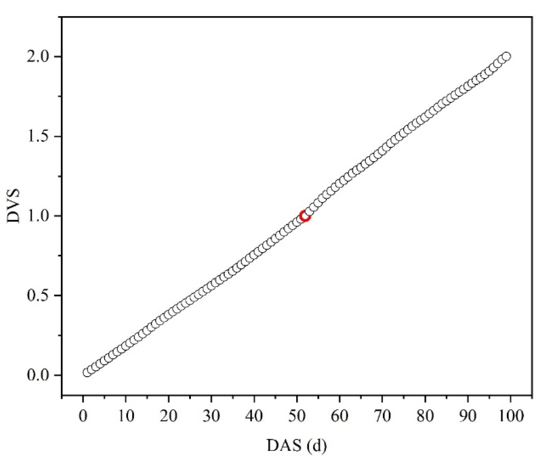
Figure 4.
Flow chart of the unified prediction framework.
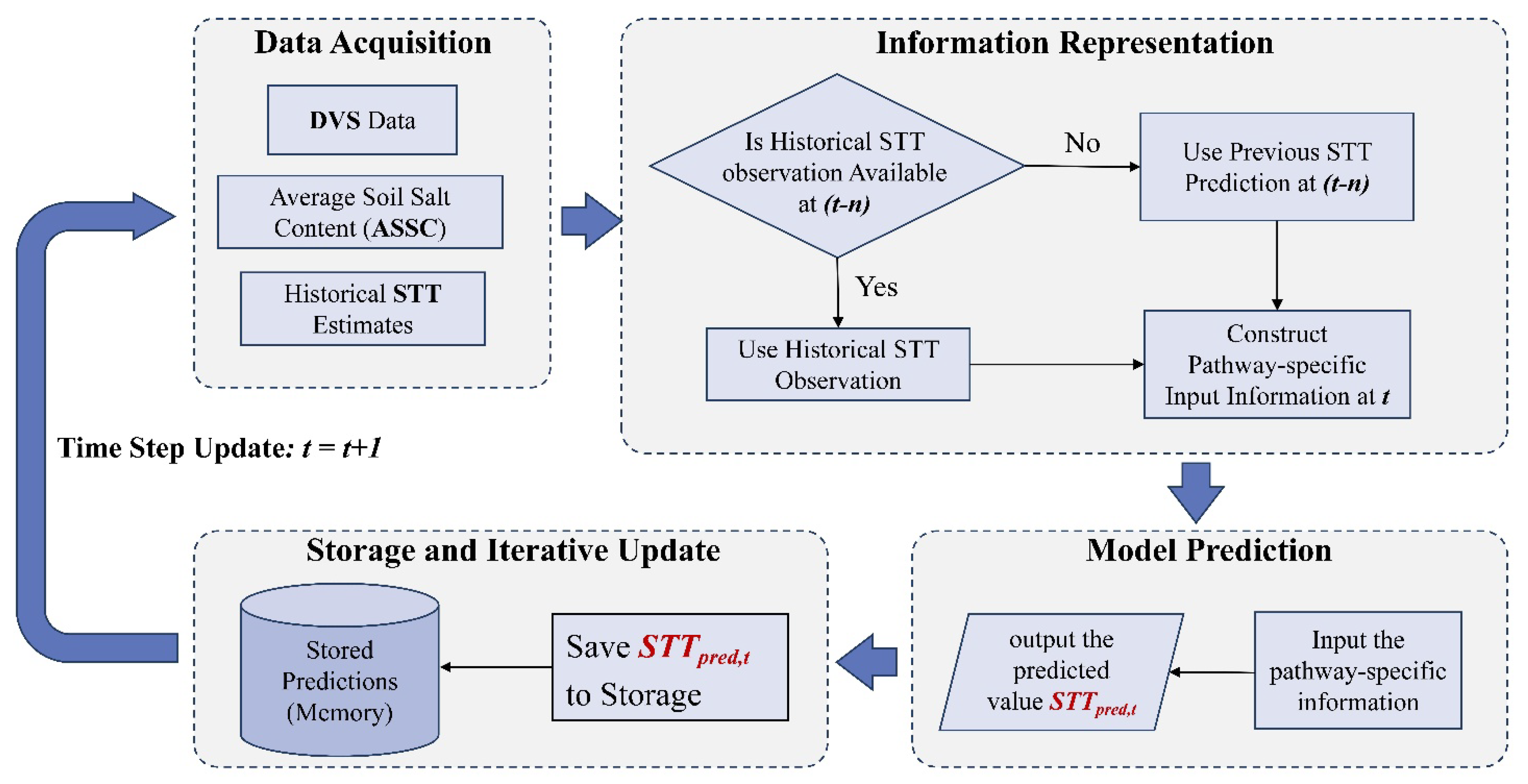
Figure 5.
Dynamic changes in photosynthetic characteristics of summer maize under brackish water irrigation during the entire growth period. The data are averaged measurements (n= 4), and vertical bars indicate standard error. The S0, S1, S2, and S3 represent different salt concentration levels of irrigation water, corresponding to none (0.08 g·L-1), mild (2.0 g·L-1), moderate (4.0 g·L-1), and severe (6.0 g·L-1) stress. DAS is the abbreviation for days after sowing.
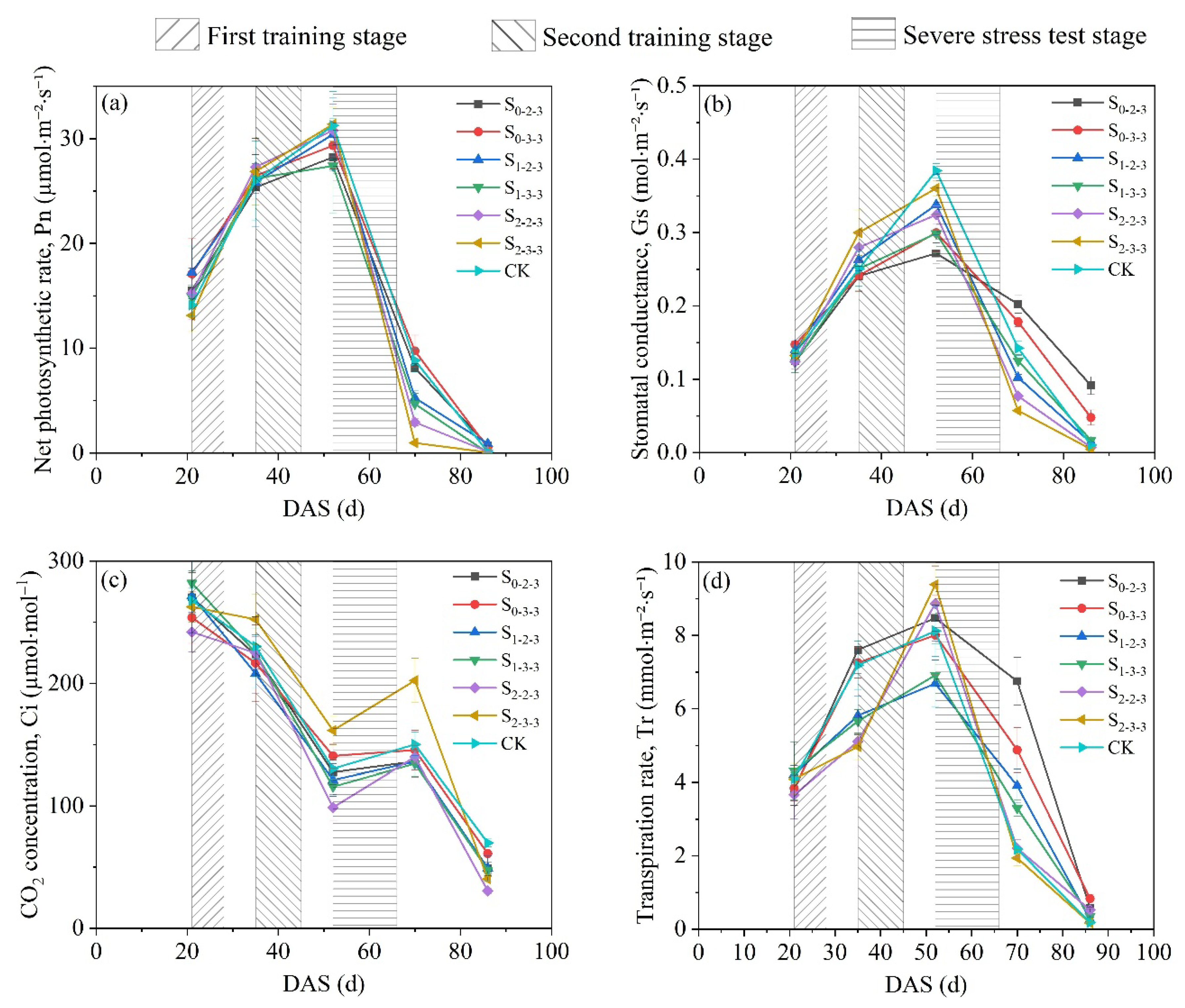
Figure 6.
Pearson correlation analysis of physiological regulatory substance indicators in summer maize at the first training stage (FTS) under three salinity levels (S0, S1, and S2). The upper triangle of each matrix displays the strength and sign of the correlations using ellipses, where eccentricity and color indicate the magnitude and sign (red for positive and blue for negative) of the correlation coefficients. The lower triangle presents the corresponding numerical values. The asterisk (*) indicates statistical significance at the 0.05 probability level (p < 0.05). S0, S1, and S2 represent different salt concentration levels of irrigation water, corresponding to none (0.08 g·L-1), mild (2.0 g·L-1) and moderate (4.0 g·L-1) stress.
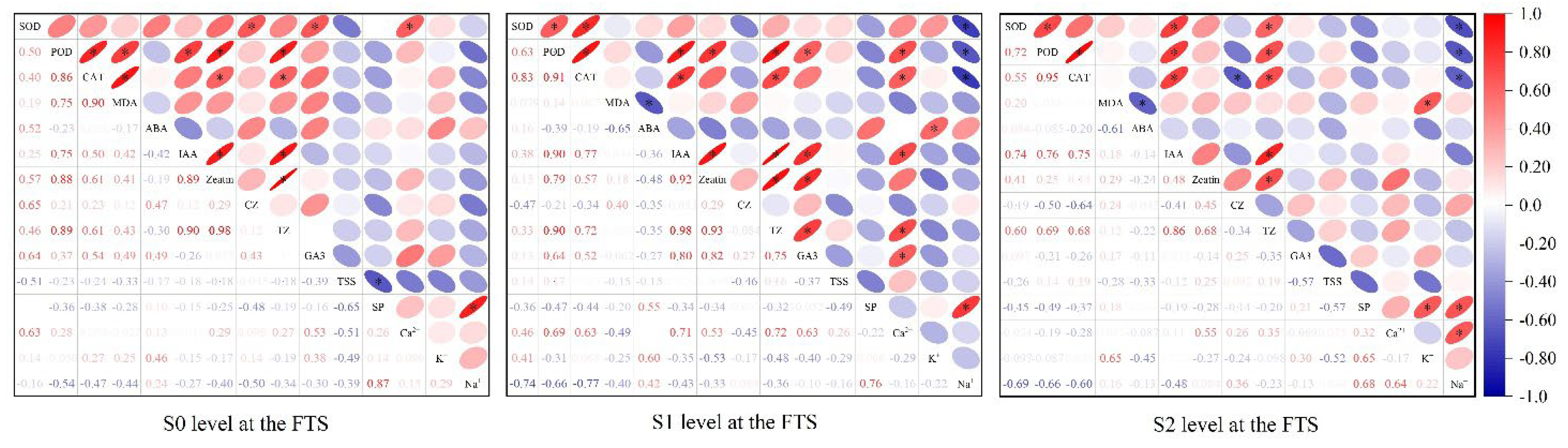
Figure 7.
Variations in CSGL, CRGL, and CLPRS.
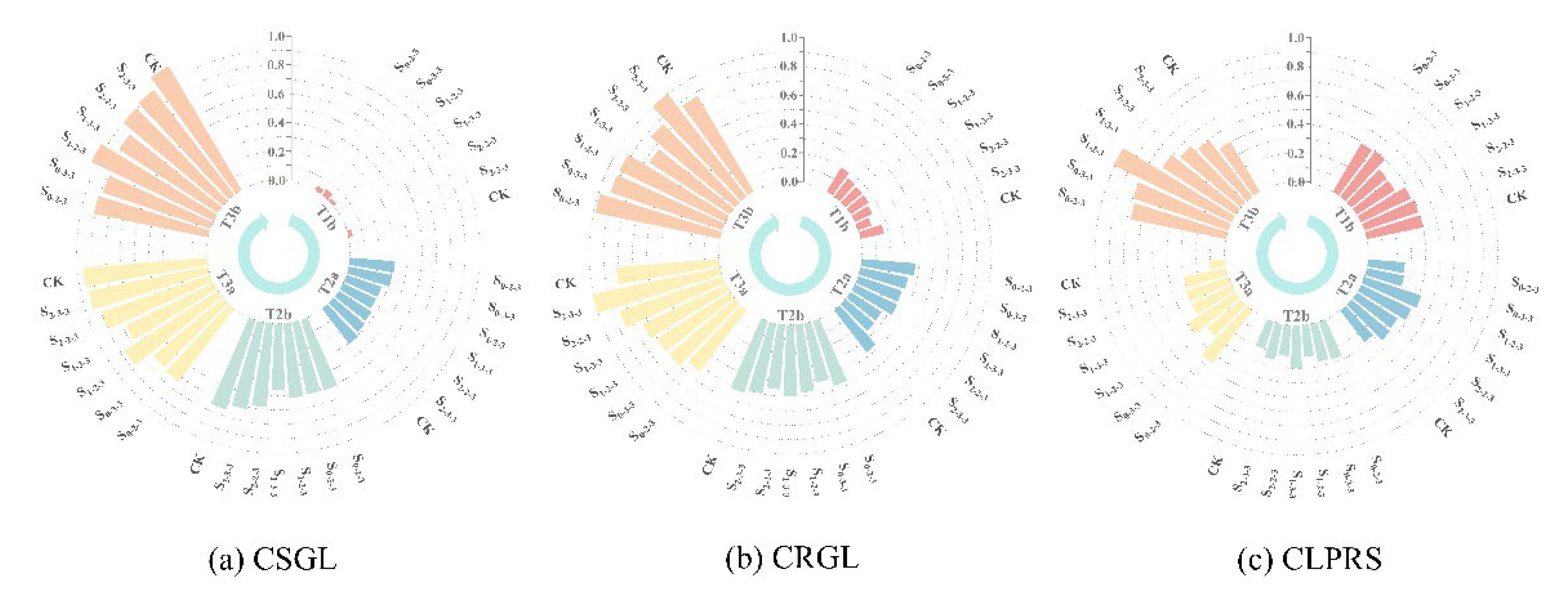
Figure 8.
Variations in average soil salt content (ASSC) within the 0–40 cm rootzone soil.
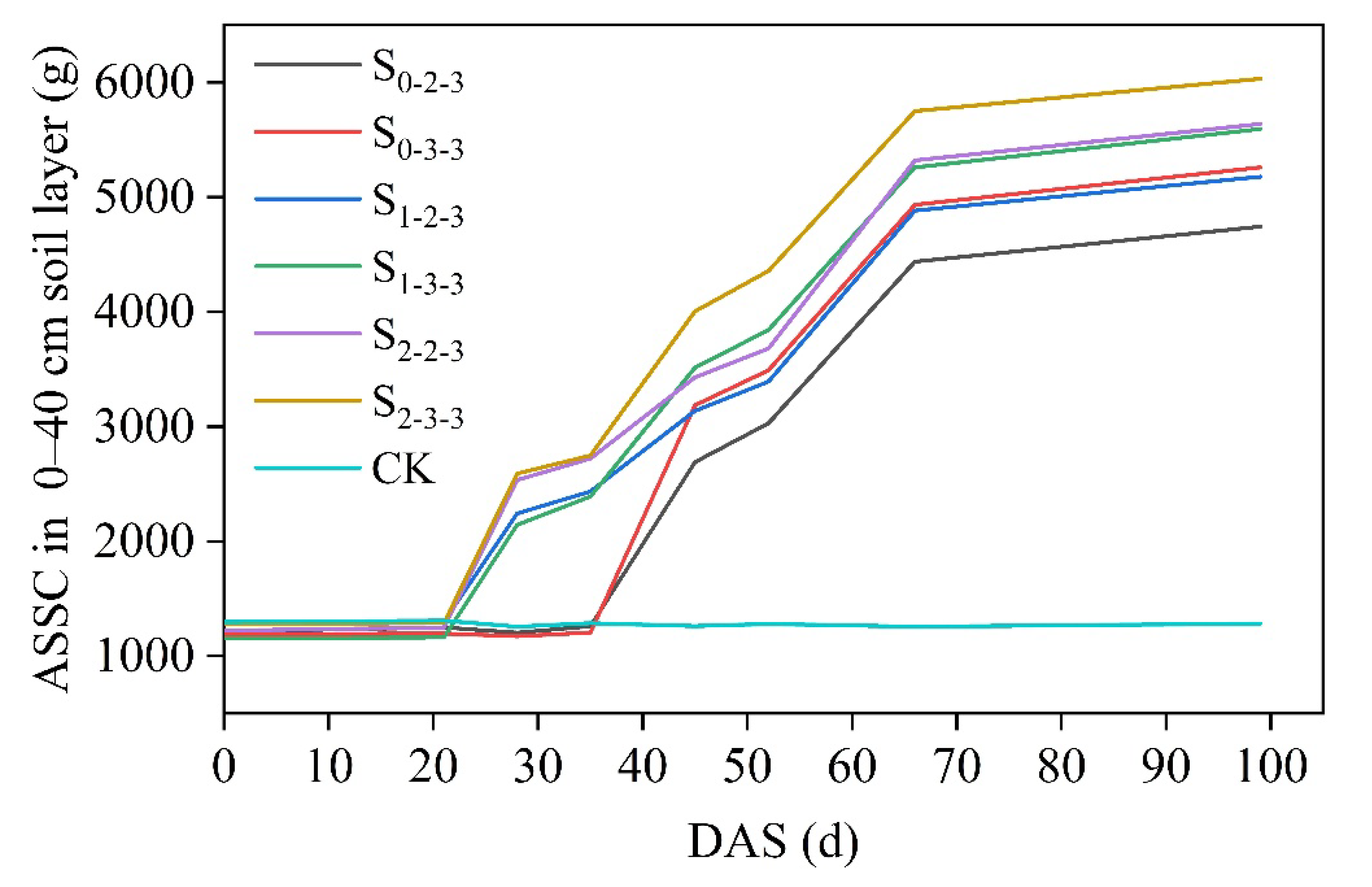
Figure 9.
Kernel density plots of measured versus predicted STT under different modeling pathways and algorithms. Regions with warmer colors correspond to areas of higher data point density.
Figure 9.
Kernel density plots of measured versus predicted STT under different modeling pathways and algorithms. Regions with warmer colors correspond to areas of higher data point density.
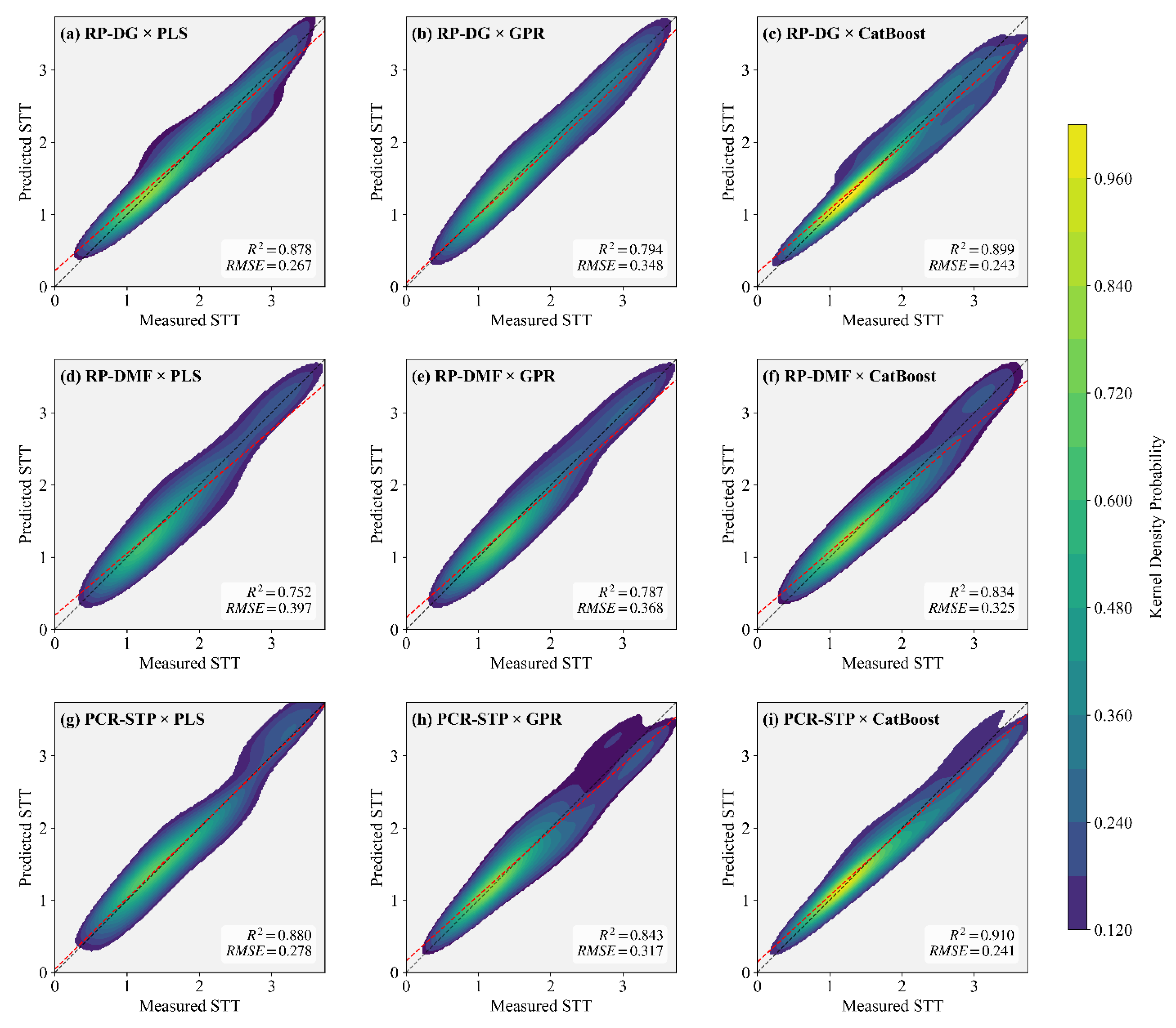

Table 1.
Basic properties of the experimental soil at 0~60 cm depth.
| Depth | Bulk density | Total nitrogen |
Organic carbon | Alkali- Hydro Nitrogen |
Available phosphorus | Available potassium | pH |
|---|---|---|---|---|---|---|---|
| cm | g·cm-3 | g·kg-1 | g·kg-1 | mg·kg-1 | mg·kg-1 | mg·kg-1 | |
| 0~10 | 1.34 | 0.69 | 4.1 | 79.7 | 14.6 | 156 | 7.14 |
| 10~20 | 1.37 | 0.68 | 4.2 | 68.0 | 11.5 | 125 | 7.36 |
| 20~30 | 1.42 | 0.64 | 3.6 | 57.5 | 10.8 | 147 | 7.51 |
| 30~40 | 1.48 | 0.67 | 4.1 | 49.8 | 14.9 | 160 | 7.31 |
| 40~50 | 1.51 | 0.65 | 2.2 | 46.4 | 12.7 | 163 | 7.40 |
| 50~60 | 1.55 | 0.66 | 3.3 | 45.1 | 11.4 | 173 | 7.53 |
Table 2.
Experimental design of salt concentration levels, stages of action, and duration in each micro-plot.
Table 2.
Experimental design of salt concentration levels, stages of action, and duration in each micro-plot.
| Brackish water irrigation Regimes | Salt concentration (g·L-1) | |||||||
|---|---|---|---|---|---|---|---|---|
| First training stage (FTS) | Recovery stage | Second training stage (STS) | Recovery stage | Severe stress test stage (SSTS) | ||||
| Initial stage | Duration | Initial stage | Duration | Initial stage | Duration | |||
| Six-Leaf stage | 21~28 DAS1 | Ten-Leaf stage | 35~45 DAS | Tasseling stage | 52~66 DAS |
|||
| S0-S2-S3(S0-2-3) | 0 | 0 | 4.0 | 0 | 6.0 | |||
| S0-S3-S3 (S0-3-3) |
0 | 0 | 6.0 | 0 | 6.0 | |||
| S1-S2-S3 (S1-2-3) |
2.0 | 0 | 4.0 | 0 | 6.0 | |||
| S1-S3-S3 (S1-3-3) |
2.0 | 0 | 6.0 | 0 | 6.0 | |||
| S2-S2-S3 (S2-2-3) |
4.0 | 0 | 4.0 | 0 | 6.0 | |||
| S2-S3-S3 (S2-3-3) |
4.0 | 0 | 6.0 | 0 | 6.0 | |||
| CK (S0-0-0) |
0 | 0 | 0 | 0 | 0 | |||
1 DAS means days after sowing.
Table 3.
Measurement time points and codes for key physiological regulatory indicators (reference for data alignment).
Table 3.
Measurement time points and codes for key physiological regulatory indicators (reference for data alignment).
| Measurement time | Code |
|---|---|
| Onset of first training stage (at the onset of the six-leaf stage) |
T1a |
| Completion of first training stage | T1b |
| Onset of second training stage (at the onset of the ten-leaf stage) |
T2a |
| Completion of second training stage | T2b |
| Onset of severe stress test stage (at the onset of the tasseling stage) |
T3a |
| Completion of severe stress test stage (during the silking stage) |
T3b |
These time points served as a reference for aligning shoot and root growth indicators in subsequent analyses.
Table 4.
Principal component analysis (PCA) results and component matrix for CLPRS, CSGL, and CRGL.
| CLPRS | CSGL | CRGL | |||||
|---|---|---|---|---|---|---|---|
| Principal Component | PC1 | PC2 | PC3 | PC1 | PC1 | PC2 | |
| Eigenvalue | 3.798 | 1.903 | 1.136 | 5.474 | 7.063 | 1.762 | |
| Contribution Rate/% | 47.473 | 23.788 | 14.206 | 91.240 | 58.856 | 14.680 | |
| Cumulative Contribution Rate/% | 47.473 | 71.261 | 85.467 | 91.240 | 58.856 | 73.536 | |
| Component Matrix | X1 | 0.903 | -0.051 | -0.139 | 0.993 | 0.813 | 0.185 |
| X2 | 0.970 | 0.036 | -0.048 | 0.984 | 0.802 | 0.091 | |
| X3 | 0.865 | 0.259 | 0.011 | 0.957 | 0.904 | -0.064 | |
| X4 | 0.878 | 0.227 | 0.150 | 0.954 | 0.896 | -0.219 | |
| X5 | 0.037 | -0.677 | 0.672 | 0.914 | 0.812 | 0.136 | |
| X6 | 0.350 | 0.563 | 0.565 | 0.927 | 0.690 | 0.559 | |
| X7 | -0.526 | 0.550 | 0.519 | —— | 0.767 | -0.117 | |
| X8 | -0.351 | 0.839 | -0.228 | —— | 0.689 | -0.575 | |
| X9 | —— | —— | —— | —— | 0.610 | 0.441 | |
| X10 | —— | —— | —— | —— | 0.671 | 0.597 | |
| X11 | —— | —— | —— | —— | 0.754 | -0.263 | |
| X12 | —— | —— | —— | —— | 0.741 | -0.609 | |
For CLPRS, X1–X8 correspond to CAT, POD, IAA, TZ, TSS, Ca²⁺, Na⁺, and SP, respectively. For CSGL, X1–X6 denote H, LAI, SB, Pn, Tr, and Gs, respectively. For CRGL, X1–X4 refer to FRLD within the 0–10, 10–20, 20–30, and 30–40 cm depth intervals, X5–X8 denote fine root surface area across the same depth intervals, and X9–X12 represent fine root biomass within the corresponding depth intervals.
Table 5.
Changes in the dynamic salt tolerance coefficient (αSTT) across growth stages.
| Treatment | 28 DAS | 35 DAS | 45 DAS | 52 DAS | 66 DAS |
|---|---|---|---|---|---|
| S0-2-3 | 1 | 1 | 0.7 | 0.7 | 0.9 |
| S0-3-3 | 1 | 1 | 0.7 | 0.8 | 0.9 |
| S1-2-3 | 0.6 | 0.7 | 0.85 | 0.9 | 1 |
| S1-3-3 | 0.6 | 0.7 | 0.85 | 0.9 | 0.9 |
| S2-2-3 | 0.7 | 0.7 | 0.8 | 1 | 0.85 |
| S2-3-3 | 0.7 | 0.7 | 0.85 | 1 | 0.85 |
Table 6.
Quantitative assessment of summer maize salt tolerance threshold (STT) across growth stages, expressed as soil salinity (g·kg⁻¹).
Table 6.
Quantitative assessment of summer maize salt tolerance threshold (STT) across growth stages, expressed as soil salinity (g·kg⁻¹).
| Treatment | 0 DAS | 21 DAS | 28 DAS | 35 DAS | 45 DAS | 52 DAS | 66 DAS |
|---|---|---|---|---|---|---|---|
| S0-2-3 | 1.30 | 1.30 | 1.35 | 1.41 | 1.50 | 1.60 | 2.65 |
| S0-3-3 | 1.30 | 1.30 | 1.35 | 1.40 | 1.53 | 1.91 | 2.94 |
| S1-2-3 | 1.30 | 1.30 | 1.35 | 1.42 | 1.83 | 2.09 | 3.35 |
| S1-3-3 | 1.30 | 1.30 | 1.34 | 1.41 | 2.05 | 2.37 | 3.25 |
| S2-2-3 | 1.30 | 1.30 | 1.36 | 1.44 | 1.88 | 2.52 | 3.10 |
| S2-3-3 | 1.30 | 1.30 | 1.36 | 1.44 | 2.33 | 2.99 | 3.35 |
| CK | 1.30 | 1.30 | 1.36 | 1.41 | 1.50 | 1.56 | 1.70 |
Disclaimer/Publisher’s Note: The statements, opinions and data contained in all publications are solely those of the individual author(s) and contributor(s) and not of MDPI and/or the editor(s). MDPI and/or the editor(s) disclaim responsibility for any injury to people or property resulting from any ideas, methods, instructions or products referred to in the content. |
© 2026 by the authors. Licensee MDPI, Basel, Switzerland. This article is an open access article distributed under the terms and conditions of the Creative Commons Attribution (CC BY) license (http://creativecommons.org/licenses/by/4.0/).
Copyright: This open access article is published under a Creative Commons CC BY 4.0 license, which permit the free download, distribution, and reuse, provided that the author and preprint are cited in any reuse.


