
Submitted:
25 January 2026
Posted:
26 January 2026
You are already at the latest version
Abstract
Accurate carbon emission forecasting is crucial for achieving the “dual-carbon” goals and supporting effective emission-reduction strategies. However, carbon emissions are affected by multiple factors (e.g., industrial structure, energy consumption, and meteorological conditions), resulting in strong nonlinearity and time-varying dynamics. Traditional forecasting models often struggle to jointly capture long-term dependencies and local variations in time series. To address this challenge, this paper proposes a novel deep learning framework based on Multi-Scale Temporal Patches (MSTP). The framework segments long sequences into interrelated temporal patches to enable fine-grained representation and multi-scale feature extraction while maintaining cross-patch dependencies. The model combines a Mamba backbone with an enhanced Local Window Transformer (LWT) mechanism, supporting carbon emission forecasting for 48–720 future time steps. Experiments against baseline models, including the standard Transformer and its variants, show that the proposed method achieves an average MSE of 0.1288 across multiple horizons, yielding an approximately 50.4% relative reduction in MSE compared with the strongest baseline, Informer. Ablation studies further confirm the substantial contributions of MSTP, Mamba and LWT to prediction accuracy. Overall, this hybrid architecture improves forecasting performance and provides technical support for sustainable energy planning and real-time emission scheduling.
Keywords:
carbon emission modeling
; time series decomposition
; MSTP
; mamba
; LWT
1. Introduction
Amid the intensifying global climate crisis, achieving carbon neutrality has emerged as a core strategic objective and a widely recognized consensus within the international community in response to climate change [1,2]. Nevertheless, industrial carbon emissions are driven by a complex interplay of factors—including industrial structure, energy efficiency, technological upgrading, and regional development imbalance—so their time series often exhibit strong dynamics, pronounced heterogeneity across industries and regions, and high-noise characteristics caused by measurement and reporting errors [3,4]. Under such circumstances, high-precision carbon emission forecasting not only facilitates early identification of potential emission fluctuations and risks but also provides scientific support for governments in formulating differentiated mitigation policies, enterprises in implementing energy-saving and emission-reduction measures, and regulatory bodies in conducting dynamic monitoring [5,6].
In recent years, modeling methods for carbon emission forecasting have continuously evolved, showing a clear trend from traditional approaches toward intelligent and integrated modeling frameworks. This trajectory has progressed from traditional statistical models to machine learning methods and deep learning models, and more recently to higher-level frameworks that integrate multi-source information and structural innovations [7]. Early studies primarily employed models such as Linear Regression [8], Autoregressive Integrated Moving Average (ARIMA) [9], and Grey Forecasting GM(1,1) [10] for trend estimation. These models are built upon linear relationships and fixed structural assumptions, offering good interpretability and ease of implementation. However, they are insufficient in capturing the nonlinear evolution and abrupt shifts induced by energy structural adjustments, policy interventions, and climate variability in real-world carbon emission data. To overcome the constraints of linear assumptions, researchers introduced Support Vector Regression (SVR) [11], Random Forest (RF) [12], and Artificial Neural Networks (ANN) [13]. These approaches made significant progress in modeling complex features and nonlinear mappings, markedly improving prediction accuracy. However, they often neglect the long-term dependency structures inherent in time series data and lack a systematic capability to model the dynamic processes of carbon emission evolution.
With the advancement of deep learning technologies, models such as Long Short-Term Memory (LSTM) [14], Gated Recurrent Unit (GRU) [15], and CNN–LSTM hybrids [16] have been widely adopted for carbon emission forecasting tasks. These models rely on recurrent or convolutional architectures to model time series, offering strong nonlinear fitting abilities and effective short-term dependency capture. While they significantly improve modeling accuracy for complex carbon emission data, they still face several limitations in practical applications. First, although LSTM and GRU alleviate the gradient vanishing problem to some extent through gating mechanisms, their memory mechanisms still suffer from information decay when handling very long sequences, limiting their ability to capture long-term trends and cross-period features. In carbon emission forecasting, policy interventions and energy structure transitions often cause slow-moving shifts across years, which these models may fail to respond to effectively. Second, hybrid models like CNN–LSTM, while adept at extracting local features and short-term dynamics, are less robust when confronted with multi-scale disturbances and non-stationary behaviors (e.g., extreme weather events or sudden production restrictions), and may overfit or mispredict under such conditions. Moreover, carbon emission data typically exhibit pronounced multi-source heterogeneity (e.g., industry-level differences, geographic disparities, and climatic factors), and many RNN/CNN-based models lack explicit mechanisms to model asymmetric variable relationships or dynamic dependencies, resulting in limited generalization capacity.
To address long-range dependency capture, Transformer [17] and its variants have been introduced into time series forecasting. While Transformer demonstrates strong capabilities in modeling long sequences, its quadratic computational complexity poses challenges for applications involving high-frequency, long-horizon time series data such as carbon emissions. To alleviate this, Informer [18] introduces the ProbSparse attention mechanism, reducing the computational burden of attention calculations and improving modeling efficiency for long sequences. However, due to its sparse attention strategy, Informer may overlook critical local perturbations—such as sudden policy changes or extreme climate events—reducing sensitivity to turning points and negatively affecting forecasting accuracy. On the other hand, Autoformer proposed by Wu et al. [19] integrates autocorrelation mechanisms and time series decomposition modules, separating sequences into trend and seasonal components to enhance periodic modeling and achieving superior performance on long-period datasets. However, carbon emission time series often contain frequent non-periodic disturbances (e.g., policy shifts) and structural changes (e.g., industrial transformation). Autoformer’s reliance on stable and separable trends and seasonality may lead to decomposition bias, limiting its robustness and generalizability in complex industrial settings.
Despite these advances, directly transferring existing Mamba-based time-series models to industrial carbon-emission forecasting remains nontrivial. First, many Mamba-based pipelines treat multivariate dimensions as generic channels or even assume channel independence for scalability, which is inadequate when heterogeneity is structured (e.g., industry–region hierarchies and heterogeneous responses to policy and climate drivers). More broadly, current multi-scale solutions lack a unified, quantitative standard for temporal resolution and therefore cannot reconcile long-term trends with short-term dynamics in a principled way; this often leads to brittle, manually tuned segmentation and aggregation across resolutions. SST(Sec. 2) addresses these challenges through practical mechanisms including configurable patching and explicit trend–residual decomposition, which separates long-term components from short-term fluctuations and supports differentiated modeling of multi-scale structure.
Second, local shocks and high-frequency perturbations are central to carbon-emission dynamics, but common Transformer-style local-attention mechanisms typically assume neighborhood stationarity and are not optimized for abrupt events; empirical work in energy forecasting indicates that additional frequency aggregation or hierarchical designs are often needed to recover sudden changes, implying that a purely global backbone can under-represent transients. To mitigate this, SST employs local-window attention with residual-attention support, together with a dual-branch short-encoder design (trend vs. residual), providing a practical pathway to preserve short-lived signals while maintaining global context. Overall, because carbon emissions arise from interacting policy, production, and equipment processes that produce multi-scale coupling and local perturbations, SST’s combination of configurable patching, explicit trend–residual modeling, and locality-aware sequence encoding offers a practical route toward improved robustness for industrial carbon-emission forecasting.
2. Overall Architecture of SST
The State Space Transformer (SST) [29] innovatively integrates the efficient state space modeling capability of Mamba with a variant of the attention mechanism derived from the Transformer architecture. Specifically, the State Space module in the model is powered by Mamba, which can precisely capture stepwise emission mutations caused by policy interventions. Meanwhile, local variation modeling is achieved through a windowed attention mechanism, reinforcing the model’s ability to express Industrial cyclical fluctuations and short-term peaks.
The SST model is composed of five primary modules:
- Multi-Scale Temporal Patcher,
- Global Patterns Expert,
- Local Variations Expert,
- Long-Short Router,
- Forecasting Module.
The overall architecture is illustrated in Figure 1. The Multi-Scale Temporal Patcher transforms the input time series into different resolutions based on the nature of the input data. The Global Patterns Expert focuses on extracting long-term patterns from low-resolution temporal data, while the Local Variations Expert specializes in capturing short-term fluctuations from high-resolution sequences. The Long-Short Router dynamically learns the contribution weights of both experts to achieve feature fusion. Finally, the fused features are passed through the prediction module, which consists of linear layers, to generate the final forecasting results.
2.1. Multi-Scale Temporal Patch – MSTP
The MSTP module primarily performs block-wise segmentation of the original temporal window data, aggregating continuous time series into sub-sequence patches. different resolutions are then assigned to long-range and short-range sequences accordingly. Specifically, for each univariate time series , the Patches process transforms it into , where L denotes the length of the original sequence, P is the patch length, and Str is the patch stride. The number of patches N can be calculated using Equation (1):
To facilitate resolution measurement in the temporal domain, the model adopts the concept of image resolution and defines a resolution metric for time series patches, denoted as (Patched Time Series Resolution). It is computed using Equation (2):
In the formula, L≫P, L≫Str. Since L is a fixed constant, it has no effect on the resolution comparison of different patching strategies (P,Str). Therefore, focusing on the regulatory effect of P and Str on resolution, after removing the fixed constant L, a simplified approximation is finally obtained.
In practical applications, the Mamba module, which is designed to identify long-term trends, processes distant sequence segments using a lower value to ensure a coarse-grained view of long-range dependencies. In contrast, the LWT module, which focuses on capturing local variations, handles near-term data with a higher value to ensure fine-grained sensitivity to short-term fluctuations.
For unpatched raw sequences (i.e., when P=1 and Str=1), the corresponding resolution equals 1 as per Equation (2). Through Multi-Scale resolution adjustment, the MSTP module addresses the limitation of raw data in distinguishing between long-term and short-term features, thereby laying a solid foundation for efficient feature extraction by the two expert modules that follow.
2.2. Global Patterns Expert
To effectively capture long-term trends and cross-period dependencies in carbon emission sequences, the SST model adopts Mamba [20] as the core of the Global Trend Modeling Unit. Mamba is a selective State Space Model (SSM) architecture built upon the classical SSM framework [30]. While classical SSM provide a solid theoretical basis for sequential modeling, their linear time-invariant assumptions and fixed parameterization limit their capacity to represent non-stationary dynamics; moreover, directly scaling classical SSMs to high-dimensional settings is often challenging. Mamba addresses these issues by introducing input-dependent (selective) parameterization, enabling content-adaptive state transitions for complex sequences.
As illustrated in Figure 2, the embedded long-term sequence is first mapped by Linear 1 (input projection) and then split into two parallel streams: a content stream and a gating stream. The content stream is processed by a lightweight local-mixing module (Conv → SILU→ SSM) before entering the Selective scan, which performs long-range state space modeling efficiently. Crucially, the “selective” mechanism comes from generating the SSM parameters from the content features: after the Conv–SILU-SSM block, a projection produces three groups of input-dependent parameters . Here, and respectively control how the current input is injected into the state and how the state is read out to form the output, while is a low-rank step-size representation that is further mapped to the discretization step through a learnable projection followed by a positivity constraint, i.e., , ensuring for valid discretization. In contrast, the state dynamics base and the skip/residual term are learnable parameters shared across time, where as are input-dependent and vary with tokens, allowing Mamba to adaptively adjust state transition paths under non-stationary carbon emission signals.
The gating stream passes through SILU to generate a content-aware modulation signal, and the output of the selective scan is combined with this gate via element-wise multiplication (the “×” node in Figure 2), i.e., . Finally, the gated representation is mapped back by Linear 2 (output projection) to obtain the global trend features used by subsequent modules. Benefiting from the hardware-aware selective scan implementation, Mamba achieves near-linear scaling with respect to sequence length (linear-time selective scan in practice), making it suitable for long-horizon industrial carbon emission forecasting. Since temporal ordering is inherently preserved by the recurrent state transition in the scan, SST does not introduce additional positional encoding after the embedding stage.
To achieve robust modeling of cross-period dependencies and suppress noise within time series, SST constructs the global trend modeling unit centered on Mamba. Specifically, each univariate in the time-series input data is first segmented into patches, forming , and then projected into a high-dimensional space as . The embedded features are fed into the Mamba-based expert to dynamically capture long-range dependency patterns while attenuating low-amplitude noise in distant contexts. The resulting long-term trend representation is denoted as , providing global temporal context for subsequent multi-scale information fusion.
2.3. Local Variations Expert
To enhance the model’s sensitivity to short-range fluctuations and local perturbations in carbon emission sequences, SST introduces a Local Variations Expert based on an enhanced Local Window Transformer (LWT). Although vanilla Transformer attention is flexible, its global attention lacks explicit local inductive bias and incurs quadratic complexity , which may hinder practical forecasting efficiency and dilute responsiveness to localized variations. To address this issue, LWT constrains attention to a fixed local window of size (Figure 4), forcing each token to focus on nearby context and thereby strengthening local perceptual capability.
As illustrated in Figure 3, the short-term input is first segmented into patches, yielding , and then embedded into a high-dimensional representation Different from the Mamba-based global expert, LWT explicitly injects positional encoding into the embedded tokens (via the operation in Figure 3) to preserve fine-grained local order information before attention is applied. The resulting sequence is then processed by a stack of LWT blocks, each consisting of a Local Window Attention (LWA) sub-layer followed by a Feed Forward network (with standard residual connections and normalization as in Transformer blocks).
For each token at position , LWA restricts the attention computation to its local neighborhood window ,clipped to valid indices. Where w is the window size. Given the embedded sequence , the query, key, and value matrices are computed as , , and . Within each window, the attention is computed by
Where denote the query/key/value vectors restricted to the local window and is the key (and query) dimension per head. Multi-head aggregation is applied in the standard form, followed by the feed-forward sub-layer to produce the local-variation features:
As shown in Figure 4, although each LWA layer only attends within a window of size , stacking LWT layers enables cross-layer information propagation: tokens at higher layers can indirectly receive information from positions that are outside the original local window through intermediate tokens in lower layers. Consequently, the effective receptive field expands progressively with depth and can be precisely quantified as covering positions, enabling broader context integration while retaining local modeling bias.
Figure 4.
Diagram of Stacked LWT Layers Extending the Receptive Field.
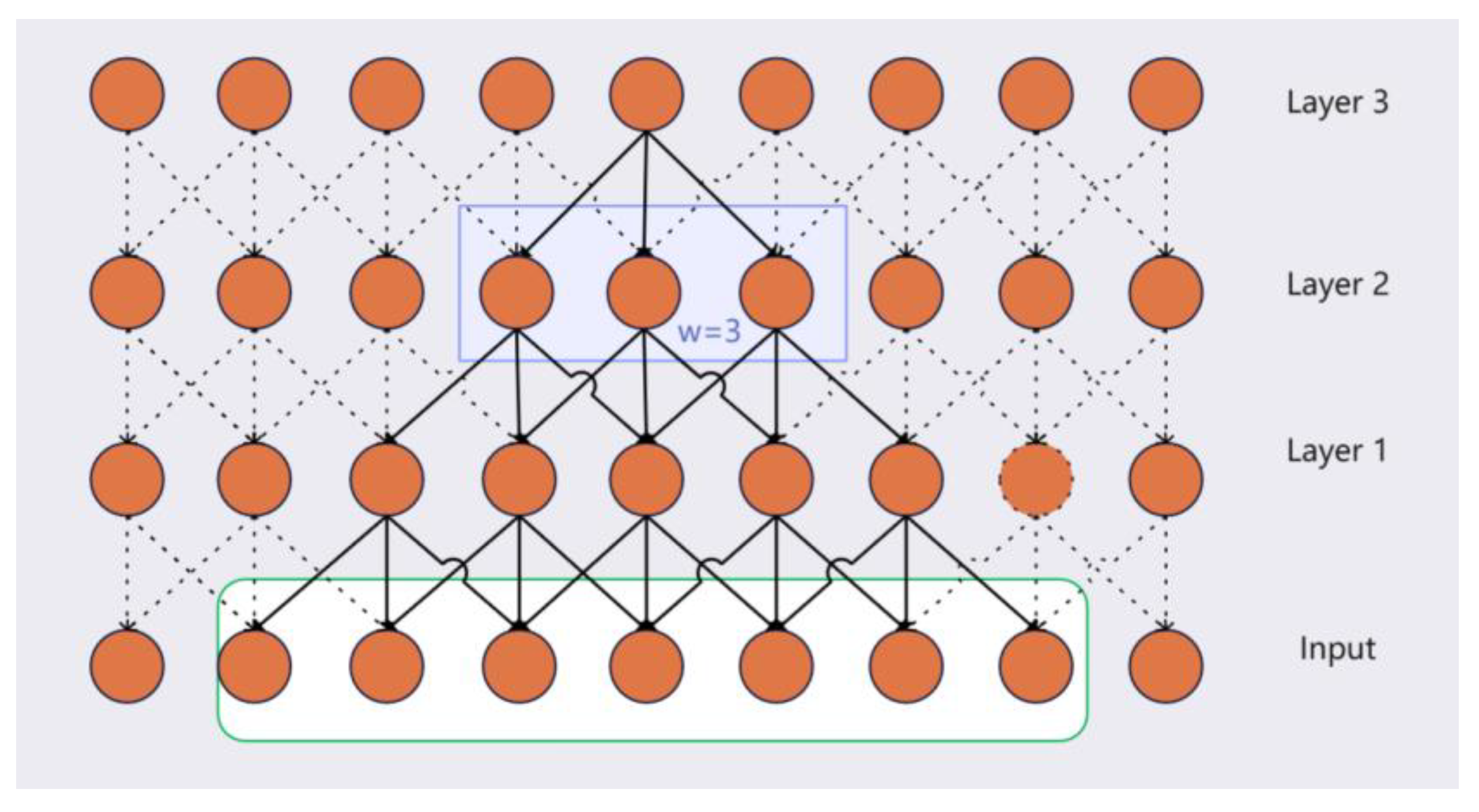
Finally, by restricting attention to local windows, the per-layer computational complexity is reduced from to for a sequence of length . This design significantly lowers computational cost and improves efficiency while maintaining strong predictive performance on local fluctuations and short-term dynamics.
2.4. Long-Short Router
The Long–Short Router is a central component in SST’s fusion architecture that adaptively balances the contributions of the Global Patterns Expert (Mamba) and the Local Window Transformer (LWT). Operating on the original input sequence , the router computes a compact sequence summary and applies a small projection followed by a softmax to produce a pair of normalized, sample-wise routing coefficients with . These coefficients quantify the model’s relative emphasis on long-term trends versus short-term variations and are used to weight the outputs of the two experts.
The router’s learned weighting is data-adaptive: for sequences dominated by stable trends or strong periodicity it tends to assign higher mass to the global expert, whereas for sequences with frequent abrupt changes it shifts mass toward the local expert. By providing a simple, interpretable gating between global and local pathways, the Long–Short Router allows SST to dynamically reweight multi–scale information according to the input’s prevailing characteristics, thereby improving robustness across heterogeneous carbon-emission series.
A concise expression of the router-guided ensemble at the feature or output level is:
where and denote the predictions (or feature-derived contributions) of the global and local experts respectively. In practice these weights are applied at the feature fusion stage to form a joint representation for the final prediction head.
2.5. Forecasting Module
The long-term trend features extracted by the Global Patterns Expert (Mamba), denoted , and the short-term variation features extracted by the Local Window Transformer (LWT), denoted , are first prepared for fusion by per-sample, per-variable flattening. Concretely, each feature map is flattened into a one-dimensional vector:
The Long–Short Router produces a pair of normalized routing coefficients with . These scalar coefficients are broadcasted to match the flattened vectors and are used to reweight the expert outputs before fusion. The weighted components are concatenated to form the fused representation:
The fused vector encodes joint information about global trends and local variations and is passed to a learned prediction head that projects it onto the -step forecasting horizon:
3. Experiments and Results
Accurate monitoring of carbon emissions is a critical prerequisite for humanity to effectively address climate change. Precise carbon emission data not only provides a solid foundation for scientific analysis but also assists policy makers in understanding the sources, intensity, and spatial distribution of emissions—thereby offering essential support for the formulation of evidence-based mitigation strategies and environmental policies[31].
However, in many regions, the lack of comprehensive monitoring systems has resulted in persistent data gaps, undermining the integrity of the global carbon emission data chain and threatening ecological balance as well as broader sustainable development goals. Against this backdrop, the value of accurate carbon emission forecasting becomes increasingly prominent: it enables proactive guidance for energy structure transformation and enterprise-level low-carbon transitions, facilitates the balancing of emission reductions with industrial competitiveness, and serves as a tool for early warning of emission risks under extreme conditions—thus strengthening both ecosystem protection and emergency management capabilities.
3.1. Dataset
To evaluate the effectiveness of the SST model in complex scenarios such as carbon emission forecasting, this study conducts a series of experiments using a carbon emission dataset for the Rwanda region, derived from Sentinel-5P satellite observations. The dataset is publicly available on the Kaggle (https://www.kaggle.com/competitions/playground-series-s3e20/data). It covers 497 monitoring regions across Rwanda from January 2019 to December 2022, including typical carbon emission scenarios such as farmlands, urban settlements, and areas surrounding power plants, as illustrated in Figure 5. The dataset is updated at a weekly granularity. Each record includes geographic coordinates (latitude and longitude) of the monitoring site, along with seven core atmospheric parameters retrieved from Sentinel-5P satellite data—such as sulfur dioxide (SO₂) and carbon monoxide (CO)—along with various auxiliary features, including gas column densities, cloud coverage, and sensor view angles. Together, these form a multidimensional spatiotemporal feature matrix.
To systematically compare the temporal characteristics of the widely used ETTh1 dataset (Electricity Transformer Temperature) and the Rwanda dataset, we evaluate periodicity, noise intensity, and trend stationarity using three complementary diagnostics. Periodicity is quantified by the Pearson lagged autocorrelation coefficient(P_lag) at a lag that matches the sampling interval (lag = 24 for ETTh1 with hourly data, corresponding to a daily cycle; and lag = 52 for Rwanda with 7-day sampling, corresponding to an annual-scale cycle). Noise intensity is measured by a decomposition-based signal-to-noise ratio (SNR) computed from STL(Seasonal and Trend decomposition using Loess), where the structured signal is defined as trend + seasonal and the noise is defined as the residual component. Trend stationarity is assessed via the Augmented Dickey–Fuller (ADF) test on the STL-extracted trend component. As shown in Table 1.
The results reveal substantial differences between the two datasets. ETTh1 exhibits strong periodicity, achieving a Pearson autocorrelation coefficient of 0.9406 at lag 24, together with a low-noise profile (SNR = 15.10 dB). Its trend component is also stationary under a 5% significance level (ADF p = 0.0116), consistent with the relatively regular temporal structure commonly observed in electricity and temperature-related data. In contrast, the Rwanda dataset shows extremely weak periodicity at the annual-scale lag, with a Pearson autocorrelation coefficient of only 0.0129 at lag 52, and a much noisier pattern (SNR = −5.33 dB), indicating that irregular residual fluctuations dominate over structured components. The trend component of Rwanda is likewise stationary (ADF p = 6.177×10⁻³⁰). Overall, these findings suggest that the Rwanda series is characterized by weak periodic structure and pronounced volatility, highlighting more complex dependencies in real-world carbon emission data and motivating forecasting models with robust representation learning and feature disentanglement capability.
3.2. Data Preprocessing
Subsequently, we conducted data preprocessing on the carbon emission dataset from the Rwanda region. The dataset contains over 79,000 monitoring records, each comprising a 70-dimensional multivariate time series, including latitude and longitude coordinates, timestamps, and carbon emission labels.
Given the large data volume and significant noise, the following multi-dimensional feature engineering and data cleaning strategies were applied:
- A unique geographic identifier (ID) was assigned to each of the 497 subregions, establishing a spatiotemporal index;
- Seasonal attributes were extracted from the weekly timestamps (Season∈{Spring, Summer, Autumn, Winter}), and one-hot encoding was used to generate 4-dimensional standard orthogonal basis vectors;
- The dataset was grouped by ID, and for each group, a 7-day moving average (MA7) and standard deviation (SD7) of the label values were computed to capture short-term emission fluctuation patterns;
- A binary COVID-19 period indicator (is_covid) was constructed, along with a lockdown status sub-feature (is_lockdown);
- Based on the central coordinates of each region, directional rotation features were constructed from multiple azimuthal angles (e.g., rot_15_x, rot_15_y, rot_30_x, rot_30_y);
- The spherical distances between each region and five key landmarks in Rwanda were calculated using the Haversine formula;
- A K-means spatial clustering was performed on the 497 regions (K = 12), producing a clustering feature (geo_cluster); additionally, the Euclidean distance from each point to the center of its assigned cluster was calculated (geo_i_cluster, where i (1, …,12));
- Low-variance features (variance < 0.1) were filtered out, removing redundant attributes;
- For missing values within the same ID group, a forward–backward fill strategy was applied: features with >50% missing rate were discarded, and the remaining missing entries were imputed with zero values.
3.3. Experimental Setup
This study conducts a comparative evaluation of the proposed SST model against a range of time series forecasting methods using the Rwanda dataset. The selected baseline models include:
- Transformer-based architectures with self-attention mechanisms, such as Transformer, Informer, and Autoformer;
- Recurrent neural network models with encoder-decoder structures[32], including ED_RNN and ED_LSTM.
To quantitatively assess forecasting performance, we employ the following metrics: Mean Squared Error (MSE), Mean Absolute Error (MAE), and Relative Squared Error (RSE), defined as in Equation (10). Lower values for these metrics indicate better predictive performance:
Where n is the number of samples, is the ground truth, is the predicted value, and is the mean of the ground truth values. In terms of model configuration, the SST model adopts a dual-branch temporal processing mechanism:
1.For long-term dependency modeling, the Mamba module uses a low-resolution setting with (i.e., patch size ), and an input sequence length =672;
2.For short-term feature extraction, the LWT module employs a high-resolution configuration with (i.e., ), and an input sequence length =336.
The sliding window size is set to , enabling the model to support Multi-Scale forecasting tasks with output sequence lengths 。
A standardized data preprocessing pipeline is applied. The dataset is split into training, validation, and test sets in a 6:2:2 ratio. All models are implemented using the PyTorch framework, with parameters optimized using the Adam optimizer. An early stopping strategy is employed with a patience of 10 epochs to prevent overfitting. All experiments are conducted on a computation platform equipped with an NVIDIA GeForce RTX 4090D GPU (24GB VRAM).
3.4. Results and Discussion
Under the experimental settings described above, we compare the performance of the SST model against several baseline models, including Autoformer, Informer, vanilla Transformer, as well as ED_RNN and ED_LSTM, both of which are encoder-decoder-based recurrent models. The results are summarized in Table 2.
As shown in Table 2, on the multivariate-to-univariate carbon emission forecasting task using the Rwanda dataset—which is heavily affected by multi-source heterogeneity—the SST model achieves the best performance across all three evaluation metrics (MSE, MAE, and RSE). Specifically, SST yields average values of 0.1288 (MSE), 0.2310 (MAE), and 0.8850 (RSE), representing improvements of 50.4%, 32.5%, and 31.0%, respectively, over the best-performing baseline model, Informer. Further visual analysis of the prediction results (Figure 6) reveals that single-architecture models such as Autoformer, Informer, and the standard Transformer exhibit various degrees of deviation between predicted and ground truth values. Their forecast curves display high-amplitude fluctuations, indicating a greater degree of instability. In contrast, the SST model demonstrates a more stable error distribution, with significantly lower prediction errors across multiple time steps compared to all baselines (p < 0.05). This indicates superior generalization ability and predictive accuracy from a statistical standpoint.
These findings validate that the unique fusion architecture of SST not only delivers superior quantitative performance metrics in carbon emission forecasting, but also exhibits notable advantages in error control and robustness. The results confirm SST’s strong suitability and effectiveness for modeling complex time series data characterized by heterogeneous sources and non-stationary dynamics.
To further investigate how input sequence length affects model performance, we compare the SST model with Autoformer, Informer, and the standard Transformer under various long-term input lengths and corresponding short-term input lengths , while keeping the output sequence length fixed at . The performance variation under these settings is summarized in Table 3.
As shown in Table 3, while the input length increases from 96 to 672, the SST model maintains remarkably stable prediction accuracy—with MSE fluctuations limited to just 1%–3%, significantly more stable than the competing models. This robustness can be attributed to SST’s Multi-Scale hybrid architecture, enabled by the combination of the Mamba module and the LWT module. Specifically, the Mamba module excels at capturing long-range dependencies, while the LWT block is adept at extracting local short-term dynamics. Their synergy allows the model to adaptively integrate global and local features under varying input lengths, thereby maintaining stable modeling performance for carbon emission sequences.
These results demonstrate that the SST model exhibits strong robustness and generalization ability across different input time scales, enabling consistent and reliable forecasting outcomes.
In addition, we conducted a quantitative analysis of each model’s parameter size, computational resource consumption, and inference speed, as reported in Table 4. While the SST model has larger parameter size and slower inference speed due to its more complex architectural design, it achieves a notable reduction in GPU memory usage, with 14.3%–47.1% lower memory consumption compared to all baseline models except Informer. This memory efficiency highlights SST’s hardware adaptability in handling high-dimensional, long-sequence forecasting tasks, making it particularly suitable for deployment in memory-constrained scenarios such as industrial carbon monitoring and climate trend modeling.
Based on the comprehensive experimental results presented above, the SST model demonstrates outstanding performance in both forecasting accuracy and computational efficiency, largely attributed to its novel internal architectural design. First, the SST model leverages the Mamba module to capture cross-scale global dependencies. The Mamba module is inherently well-suited for parallel computation, fully exploiting the processing power of modern hardware such as GPUs. It supports parallel operations across different channels and batch dimensions, significantly improving computational throughput. This high-efficiency computation paradigm allows Mamba to effectively uncover weak periodic patterns embedded within the Rwanda dataset. In contrast, traditional models like RNN and LSTM, due to their sequential recurrence mechanisms, must process each time step in order, which severely limits their computational efficiency. Second, the SST model incorporates a Local Window Attention (LWT) mechanism to extract local abrupt variations in the time series. This window-based design not only enables precise characterization of sudden events that impact carbon emissions but also reduces the overall computational complexity. As a result, the model achieves high computational efficiency while maintaining sensitivity to local patterns. Furthermore, the Long-Short Router plays a crucial role by dynamically integrating global and local features. This routing mechanism prevents unnecessary computation caused by uniformly processing all features, enabling the model to adaptively focus on features at different temporal scales. Such adaptability ensures both precision and efficiency, allowing the SST model to operate effectively under complex and heterogeneous temporal dynamics.
3.5. Ablation Studies
In the field of carbon emission forecasting, the SST model represents the first architecture to deeply integrate Mamba with Transformer mechanisms. However, the effectiveness of this hybrid strategy in such a domain remains to be fully validated. To systematically evaluate the predictive contribution of each core component within SST, and to contrast its integration approach with the MAMBAFORMER model[33], we design a series of controlled comparative experiments. The experiment includes the following configurations:①No Mamba: An SST variant with the Mamba global trend expert module removed, used to assess the impact of long-range dependency modeling on overall forecasting performance;②No LWT: An SST variant without the LWT local variation expert module, designed to analyze the model’s ability to capture short-term local features;③No Patch: An SST variant that removes the MSTP mechanism, to validate the necessity of multi-resolution feature extraction from raw input data;④MAMBAFORMER: A baseline model using an alternative Mamba-Transformer fusion strategy;⑤Full SST: The complete SST model, serving as the experimental group.
As shown in Figure 7, the SST model demonstrates clear advantages through its dynamic integration of the Mamba and Transformer modules. The Mamba module effectively captures long-range global trends thanks to its highly efficient long-sequence modeling capability, while the LWT module, part of the Transformer architecture, focuses on subtle short-term local variations.
This complementary hybrid strategy allows the SST model to extract a more comprehensive set of temporal features, significantly outperforming both the MAMBAFORMER baseline and all ablated variants in time series forecasting tasks. These results not only confirm the superiority of SST’s fusion approach but also underscore the critical importance of each component’s contribution and their synergistic interaction in achieving high-accuracy carbon emission prediction.
4. Conclusions
In this study, we applied the SST model to the task of carbon emission forecasting and conducted extensive experiments to validate its performance. By decomposing time series data across different resolutions into global trends and local variations, SST demonstrated superior forecasting capability under complex emission scenarios. The results confirm that SST achieves high precision and efficiency by leveraging a triadic collaborative mechanism—namely, global state space modeling, local variation feature analysis, and dynamic computational resource allocation. This enables the model to accurately capture both long-term trends and short-term fluctuations in carbon emission data. Compared with existing approaches, SST establishes itself as a new state-of-the-art (SOTA) model for carbon emission forecasting, offering reliable technical support for emission trend analysis and policy formulation.
However, three focused limitations guide our next steps. First, we will systematically evaluate short-input → long-horizon robustness: run controlled experiments that shorten the input history while holding the prediction horizon fixed, and report MSE/MAE together with event-oriented metrics (spike detection recall) and ablations (Mamba-only, LWT-only, router disabled). Second, the current datasets lack critical exogenous modalities (policy texts, regional GDP). We plan to extend SST to a multimodal architecture by embedding policy documents (domain-fine-tuned language models) and economic covariates, and fusing them via cross-attention or hierarchical mixture-of-experts so the model adapts to policy/economic regime shifts. Third, to improve trust and policy relevance, we will enhance interpretability: apply post-hoc attribution (SHAP), visualize Mamba latent states and routing activations, and run counterfactual/policy-scenario analyses to reveal drivers of forecasts and support actionable decision-making. These steps aim to strengthen SST’s robustness, adaptability, and explanatory power for real-world carbon policy use.
Author Contributions
 First A. Author Yuanhao Xiong was born in China in 2001 and obtained a bachelor’s degree in logistics engineering from Shanghai Ocean University in 2023. He is currently pursuing a master’s degree in mechanical engineering at the university’s School of Engineering. His research interests include time series forecasting, carbon emission modeling, and the application of artificial intelligence. He is mainly responsible for the experiments, modeling and text writing of this article.
  Correspondence Author Meiling Wang was born in January 1987 in China. She received her Ph.D. degree in Atomic and Molecular Physics from Fudan University, Shanghai, China, in 2016. Her primary research interests focus on the development and application of high-sensitivity electromagnetic sensors, as well as AI algorithms for image and data processing. Currently, she holds the position of Associate Professor at Shanghai Ocean University. She is mainly responsible for the guidance of this article.
 Data Availability Statement
The dataset used in this study is publicly available on the Kaggle platform under the competition titled “Playground Series - Season 3, Episode 20”, accessible at:https://www.kaggle.com/competitions/playground-series-s3e20/data.All raw data used in this research were obtained from this open-access source. Prior to model training and evaluation, the dataset was subject to preprocessing procedures including feature extraction, missing value handling, and normalization, as detailed in Section 3.2 of this paper. No proprietary or restricted-access data were involved.
Acknowledgments
The author would like to acknowledge the assistance of ChatGPT, a large language model developed by OpenAI, which was used solely for language refinement and academic polishing of the English manuscript. The model was accessed via the ChatGPT platform (https://chat.openai.com), and its role was limited to improving the clarity, grammar, and fluency of the paper’s English expressions. All technical content, experimental design, and scientific analysis were independently conceived and completed by the author. This section is not mandatory but may be added if there are patents resulting from the work reported in this manuscript.
Conflicts of Interest
No potential competing interest was reported by the authors Abbreviations
References
- Wang, F; Harindintwali, J D; Yuan, Z; et al. Technologies and perspectives for achieving carbon neutrality. The innovation 2021, 2. [Google Scholar]
- Liu, Z; Deng, Z; He, G; et al. Challenges and opportunities for carbon neutrality in China. Nature Reviews Earth & Environment 2022, 3, 141–155. [Google Scholar]
- Chen, H; Wang, R; Liu, X; et al. Monitoring the enterprise carbon emissions using electricity big data: A case study of Beijing. Journal of Cleaner Production 2023, 396, 136427. [Google Scholar] [CrossRef]
- Liu, Y; Xiao, H; Zhang, N. Industrial carbon emissions of China’s regions: A spatial econometric analysis. Sustainability 2016, 8, 210. [Google Scholar] [CrossRef]
- Hu, Y; Man, Y. Energy consumption and carbon emissions forecasting for industrial processes: Status, challenges and perspectives. Renewable and Sustainable Energy Reviews 2023, 182, 113405. [Google Scholar] [CrossRef]
- Tollefson, J. China’s carbon emissions could peak sooner than forecast. Nature 2016, 531, 425–426. [Google Scholar] [CrossRef] [PubMed]
- Gao, H; Wang, X; Wu, K; et al. A review of building carbon emission accounting and prediction models. Buildings 2023, 13, 1617. [Google Scholar] [CrossRef]
- Libao, Y; Tingting, Y; Jielian, Z; et al. Prediction of CO2 emissions based on multiple linear regression analysis. Energy Procedia 2017, 105, 4222–4228. [Google Scholar] [CrossRef]
- Sharma, S; Mittal, A; Bansal, M; et al. Forecasting of carbon emissions in India using (ARIMA) time series predicting approach[C]//International Conference on Renewable Power; Springer Nature Singapore: Singapore, 2023; pp. 799–811. [Google Scholar]
- Lin, C S; Liou, F M; Huang, C P. Grey forecasting model for CO2 emissions: A Taiwan study. Applied energy 2011, 88, 3816–3820. [Google Scholar]
- Chen, Y; Xu, P; Chu, Y; et al. Short-term electrical load forecasting using the Support Vector Regression (SVR) model to calculate the demand response baseline for office buildings. Applied Energy 2017, 195, 659–670. [Google Scholar] [CrossRef]
- Rigatti, S J. Random forest. Journal of insurance medicine 2017, 47, 31–39. [Google Scholar] [CrossRef] [PubMed]
- Ahmad, A S; Hassan, M Y; Abdullah, M P; et al. A review on applications of ANN and SVM for building electrical energy consumption forecasting. Renewable and Sustainable Energy Reviews 2014, 33, 102–109. [Google Scholar] [CrossRef]
- Nie, W; Huang, Z; Mai, S; et al. Carbon emission prediction and analysis of influencing factors based on the LSTM model[C]//International Conference on Computer Graphics, Artificial Intelligence, and Data Processing (ICCAID 2024). SPIE 2025, 13560, 631–636. [Google Scholar]
- Yang, F; Liu, D; Zeng, Q; et al. Prediction of mianyang carbon emission trend based on adaptive gru neural network[C]//2022 4th International Conference on Frontiers Technology of Information and Computer (ICFTIC); IEEE; Volume 2022, pp. 747–750.
- Han, Z; Cui, B; Xu, L; et al. Coupling LSTM and CNN neural networks for accurate carbon emission prediction in 30 Chinese provinces. Sustainability 2023, 15, 13934. [Google Scholar] [CrossRef]
- Vaswani, A; Shazeer, N; Parmar, N; et al. Attention is all you need. Advances in neural information processing systems 2017, 30. [Google Scholar]
- Zhou, H; Zhang, S; Peng, J; et al. Informer: Beyond efficient transformer for long sequence time-series forecasting. Proceedings of the AAAI conference on artificial intelligence 2021, 35, 11106–11115. [Google Scholar]
- Wu, H; Xu, J; Wang, J; et al. Autoformer: Decomposition transformers with auto-correlation for long-term series forecasting. Advances in neural information processing systems 2021, 34, 22419–22430. [Google Scholar]
- Gu, A; Dao, T. Mamba: Linear-time sequence modeling with selective state spaces[C]//First conference on language modeling. 2024. [Google Scholar]
- Wang, Z; Kong, F; Feng, S; et al. Is mamba effective for time series forecasting? Neurocomputing 2025, 619, 129178. [Google Scholar] [CrossRef]
- Liang, A; Jiang, X; Sun, Y; et al. Bi-mamba+: Bidirectional mamba for time series forecasting. arXiv 2024, arXiv:2404.15772. [Google Scholar]
- Ahamed, M A; Cheng, Q. Timemachine: A time series is worth 4 mambas for long-term forecasting[C]//ECAI 2024: 27th European Conference on Artificial Intelligence, 19-24 October 2024. European Conference on Artificial Intelli, Santiago de Compostela, Spain-Including 13th Conference on Prestigious Applications of Intelligent Systems, 2024; 392, p. 1688. [Google Scholar]
- Ma, H; Chen, Y; Zhao, W; et al. A Mamba Foundation Model for Time Series Forecasting. arXiv 2024, arXiv:2411.02941. [Google Scholar] [CrossRef]
- Hong, J T; Han, S; Yan, J; et al. Dual-path Frequency Mamba-Transformer Model for Wind Power Forecasting. Energy 2025, 137225. [Google Scholar] [CrossRef]
- Shen, T; Shi, W; Lei, J; et al. PAKMamba: Enhancing electricity load forecasting with periodic aggregation and Koopman analysis. Computers and Electrical Engineering 2025, 123, 110113. [Google Scholar] [CrossRef]
- Hu, J; Duan, P; Cao, X; et al. A multi-energy load forecasting method based on the Mixture-of-Experts model and dynamic multilevel attention mechanism. Energy 2025, 324, 135947. [Google Scholar]
- Lee, J; Hong, S. Reliable Grid Forecasting: State Space Models for Safety-Critical Energy Systems. arXiv 2026, arXiv:2601.01410. [Google Scholar] [CrossRef]
- XU, X; CHEN, C; LIANG, Y; et al. SST: Multi-Scale Hybrid Mamba-Transformer Experts for Long-Short Range Time Series Forecasting; 2024. [Google Scholar]
- GU, A; JOHNSON, I; GOEL, K; et al. Combining Recurrent, Convolutional, and Continuous-time Models with Linear State-Space Layers. In Cornell University - arXiv; Cornell University - arXiv, 2021. [Google Scholar]
- Faruque, M O; Rabby, M A J; Hossain, M A; et al. A comparative analysis to forecast carbon dioxide emissions. Energy Reports 2022, 8, 8046–8060. [Google Scholar] [CrossRef]
- Cho, K; Van Merriënboer, B; Gulcehre, C; et al. Learning phrase representations using RNN encoder-decoder for statistical machine translation. arXiv 2014, arXiv:1406.1078. [Google Scholar] [CrossRef]
- XU, X; LIANG, Y; HUANG, B; et al. Integrating Mamba and Transformer for Long-Short Range Time Series Forecasting[J].
Figure 1.
SST model architecture.
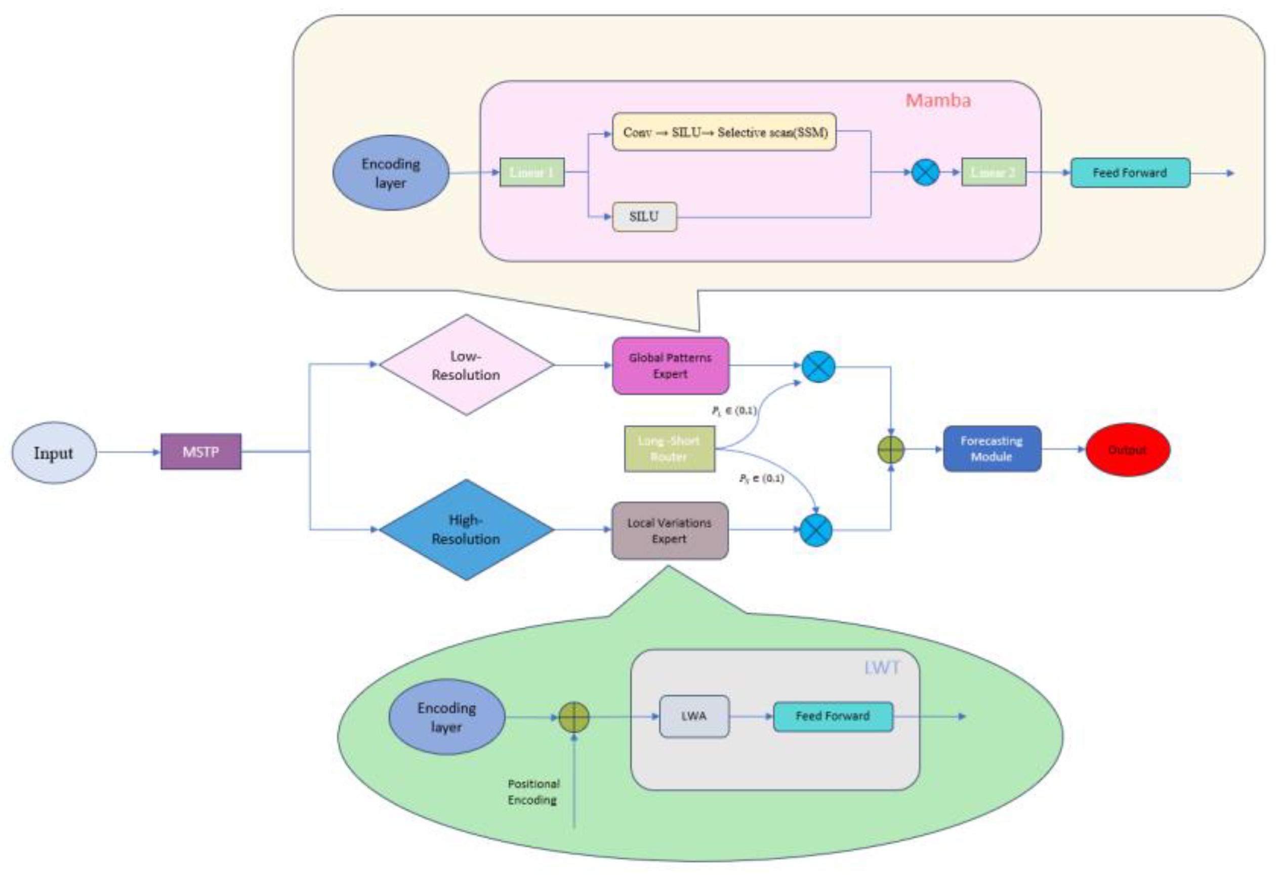
Figure 2.
Global Patterns Expert Main Structure Diagram.
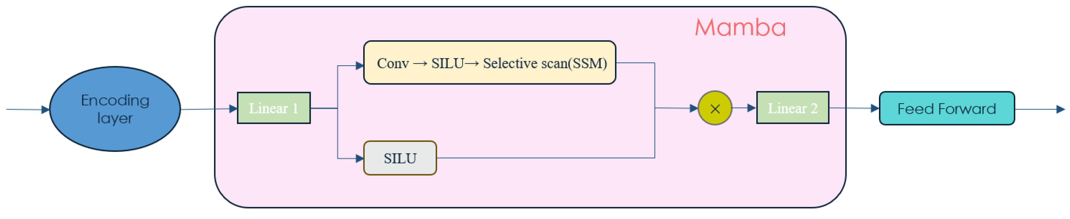
Figure 3.
Local Variations Expert Main Structure Diagram.
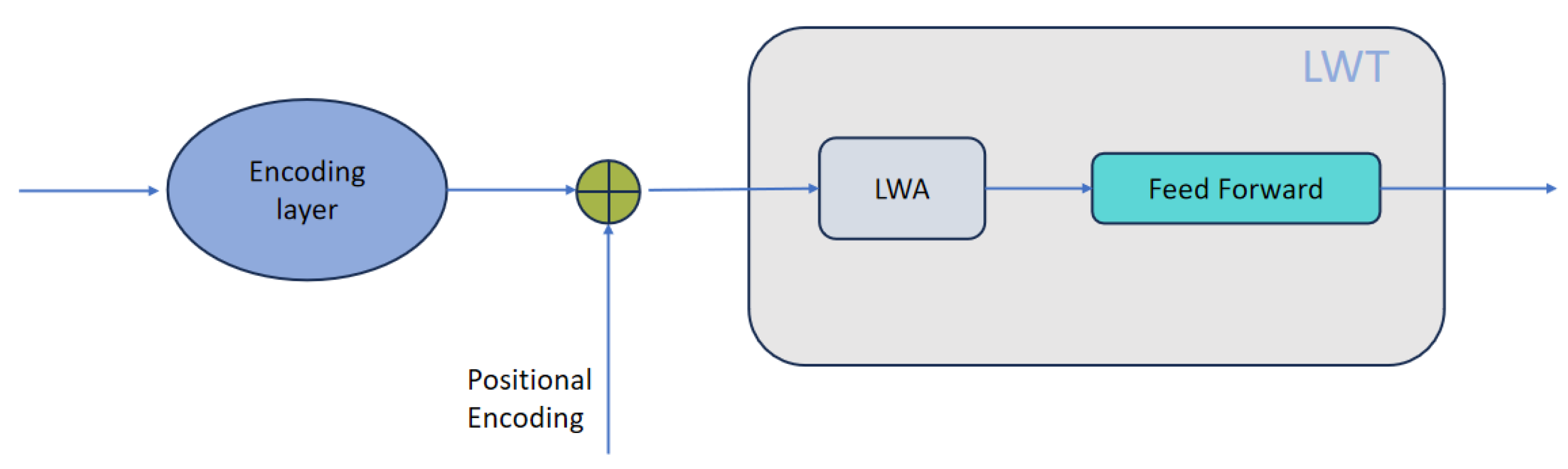
Figure 5.
Map of carbon emission observation points in the Rwanda dataset.
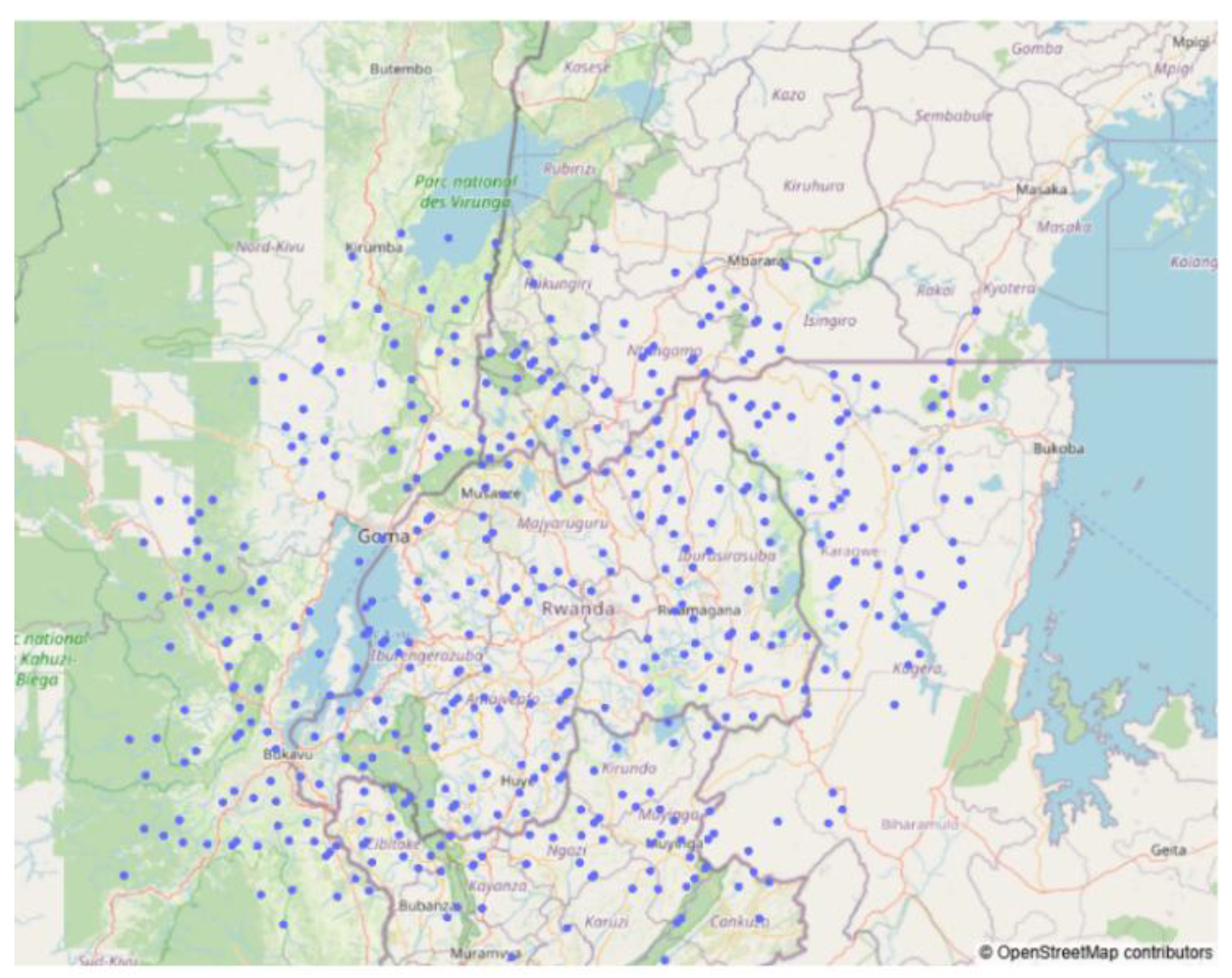
Figure 6.
Line chart of MSE, MAE and RSE loss values of each model.
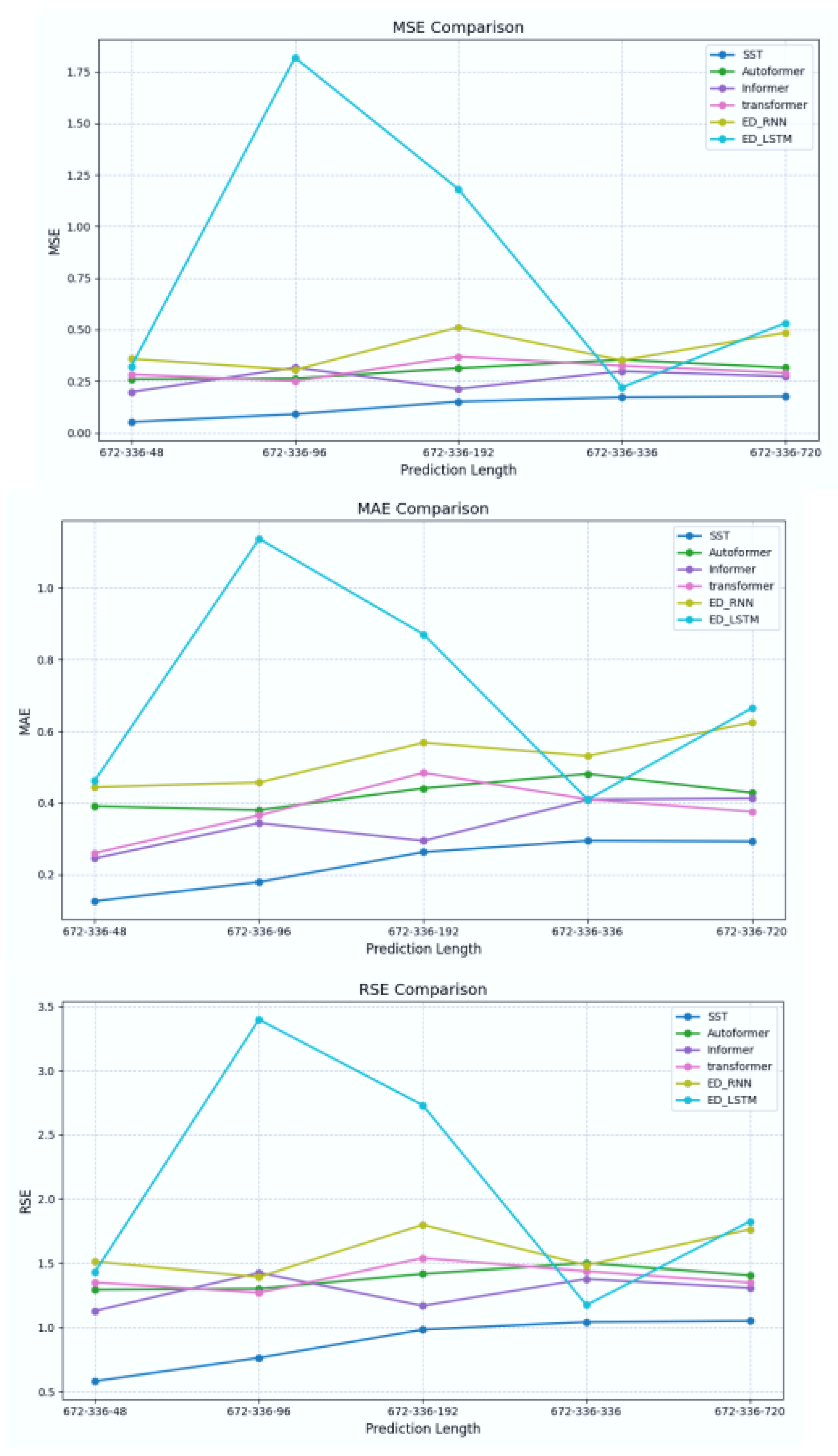
Figure 7.
=672, =336, Ablation experiment MSE average straight loss histogram under prediction length .
Figure 7.
=672, =336, Ablation experiment MSE average straight loss histogram under prediction length .
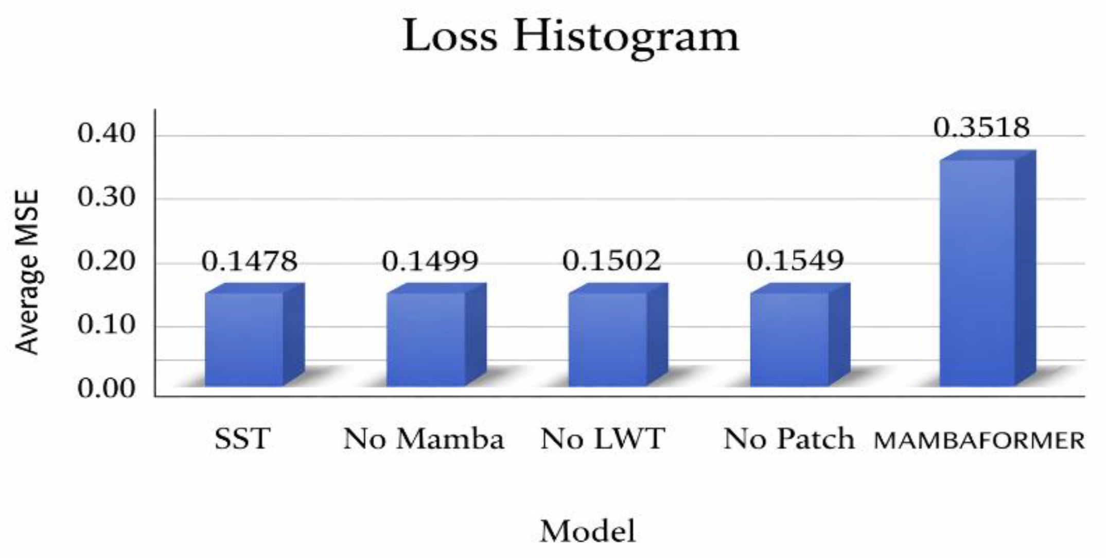

Table 1.
Comparison of periodicity, noise level (SNR), and trend stationarity (ADF) between ETTh1 and Rwanda.
Table 1.
Comparison of periodicity, noise level (SNR), and trend stationarity (ADF) between ETTh1 and Rwanda.
| Dataset | Sampling interval | Cycle | P_lag | SNR | ADF p |
|---|---|---|---|---|---|
| ETTh1 | 1 hour | 24(Daily) | 0.9406 | 15.10 | 0.0116 |
| ETTh1 | 1 hour | 168(Weekly) | 0.8701 | —— | —— |
| Rwanda | 7 days | 13(Quarter) | 0.0091 | —— | —— |
| Rwanda | 7 days | 26(Half a year) | 0.0021 | —— | —— |
| Rwanda | 7 days | 52(Annual) | 0.0129 | -5.33 | 6.177e-30 |
Table 2.
Multivariate to univariate carbon emission prediction results at different prediction lengths on the Rwanda dataset (the best results are in bold and underlined).
Table 2.
Multivariate to univariate carbon emission prediction results at different prediction lengths on the Rwanda dataset (the best results are in bold and underlined).
| -- | 672-336-48 | 672-336-96 | 672-336-192 | 672-336-336 | 672-336-720 | ||||||||||
| Model | MSE | MAE | RSE | MSE | MAE | RSE | MSE | MAE | RSE | MSE | MAE | RSE | MSE | MAE | RSE |
| SST | 0.0525 | 0.1262 | 0.5815 | 0.0905 | 0.1779 | 0.7628 | 0.1516 | 0.2631 | 0.9823 | 0.1729 | 0.2948 | 1.0474 | 0.1765 | 0.2932 | 1.0508 |
| Autoformer | 0.2602 | 0.3912 | 1.2950 | 0.2635 | 0.3803 | 1.3026 | 0.3135 | 0.4411 | 1.4176 | 0.3538 | 0.5808 | 1.5004 | 0.3157 | 0.4285 | 1.4066 |
| Informer | 0.1981 | 0.2455 | 1.1301 | 0.3162 | 0.3439 | 1.4269 | 0.2133 | 0.2943 | 1.1692 | 0.2987 | 0.4096 | 1.3787 | 0.2729 | 0.4184 | 1.3078 |
| Transformer | 0.2830 | 0.2607 | 1.3506 | 0.2510 | 0.3655 | 1.2711 | 0.3693 | 0.4839 | 1.5385 | 0.3250 | 0.4102 | 1.4380 | 0.2906 | 0.3758 | 1.3495 |
| ED_RNN | 0.3587 | 0.4444 | 1.5113 | 0.3054 | 0.4571 | 1.3929 | 0.5116 | 0.5682 | 1.7977 | 0.3515 | 0.5311 | 1.4834 | 0.4852 | 0.6245 | 1.7625 |
| ED_LSTM | 0.3228 | 0.4628 | 1.4336 | 1.8185 | 1.1364 | 3.3987 | 1.1812 | 0.8705 | 2.7316 | 0.2206 | 0.4094 | 1.1752 | 0.5324 | 0.6654 | 1.8245 |
Table 3.
Multivariate to univariate carbon emission prediction results for different input sequence lengths on the Rwanda dataset (the best results are in bold and underlined).
Table 3.
Multivariate to univariate carbon emission prediction results for different input sequence lengths on the Rwanda dataset (the best results are in bold and underlined).
| -- | 96-48-96 | 192-96-96 | 336-192-96 | 672-336-96 | ||||||||
| Model | MSE | MAE | RSE | MSE | MAE | RSE | MSE | MAE | RSE | MSE | MAE | RSE |
| SST | 0.0875 | 0.1501 | 0.7502 | 0.0887 | 0.1570 | 0.7552 | 0.0871 | 0.1682 | 0.7486 | 0.0905 | 0.1779 | 0.7628 |
| Autoformer | 0.1309 | 0.2465 | 0.8651 | 0.1883 | 0.3191 | 1.1010 | 0.2013 | 0.3293 | 1.1385 | 0.2635 | 0.3803 | 1.3021 |
| Informer | 0.2358 | 0.2558 | 1.2322 | 0.4915 | 0.3243 | 1.7789 | 0.4393 | 0.3890 | 1.6818 | 0.3162 | 0.3439 | 1.4269 |
| Transformer | 0.0951 | 0.1824 | 0.7824 | 1.0721 | 0.4214 | 2.6271 | 0.8087 | 0.4514 | 2.2817 | 0.2510 | 0.3655 | 1.2711 |
Table 4.
Comparison of model parameters, memory consumption and training time.
| Model | Total number of parameters | Memory Cost(MB) | Average time for epoch(seconds/epoch) |
| SST | 3952180 | 3386.07 | 131.32 |
| Autoformer | 2730497 | 3871.63 | 112.81 |
| Informer | 2934529 | 1384.06 | 70.41 |
| Transformer | 2737153 | 4081.15 | 88.95 |
| ED_RNN | 479745 | 6188.16 | 100.46 |
| ED_LSTM | 1127937 | 6399.59 | 112.77 |
Disclaimer/Publisher’s Note: The statements, opinions and data contained in all publications are solely those of the individual author(s) and contributor(s) and not of MDPI and/or the editor(s). MDPI and/or the editor(s) disclaim responsibility for any injury to people or property resulting from any ideas, methods, instructions or products referred to in the content. |
© 2026 by the authors. Licensee MDPI, Basel, Switzerland. This article is an open access article distributed under the terms and conditions of the Creative Commons Attribution (CC BY) license (http://creativecommons.org/licenses/by/4.0/).
Copyright: This open access article is published under a Creative Commons CC BY 4.0 license, which permit the free download, distribution, and reuse, provided that the author and preprint are cited in any reuse.


