Submitted:
16 January 2026
Posted:
21 January 2026
You are already at the latest version
Abstract
In the manuscript [1] that led to his epoch-making paper "On the Number of Primes Less Than a Given Magnitude" [2], Bernhard Riemann had already revealed the Reciprocal Sum Formula for all of the nontrivial zeros of the Riemann zeta function. We leverage this formula to prove the proposition that is our paper's title.
Keywords:
the Riemann zeta function
; Riemann Hypothesis
; the nontrivial zeros
; the twin zeros
; the tetradic zeros
; the Riemann Reciprocal Sum Formula (Constant)
1. Introduction
Prime numbers occupy a central place in number theory. They are the multiplicative building blocks of the positive integers: every integer n > 1 factors uniquely as a product of primes. This is the content of the Fundamental Theorem of Arithmetic.
In the process of understanding and researching, prime numbers seem to appear irregularly and uncannily. Although there are one-sided formulas for generating primes, such as those proposed by Euler and Mersenne, etc., it is always impossible to predict the next prime number. This very mystery has captivated many mathematicians throughout history, compelling them to devote their efforts—even their entire lives—to unraveling the patterns governing primes.
This situation was finally terminated by the great mathematician Georg Friedrich Bernhard Riemann in the mid-19th century. In his famous paper “Über die Anzahl der Primzahlen unter einer gegebenen Grösse” [2] (English: "On the Number of Primes Less Than a Given Magnitude" [3, p.299]), Riemann proved the exact expression of the prime-counting function containing all nontrivial zeros of the Riemann zeta function. But then, a new problem had emerged from Riemann’s work—the similar irregularity in the pattern of the nontrivial zeros has led countless mathematicians in various eras after Riemann to tirelessly and painfully explore the way and the mathematical laws that determine their presence.
To this day, in mathematics, it is widely known that this problem has not been completely solved.
Based mainly on the study and exploration of [1,2,3], we realize that Riemann presented two parts of content in his notable 1859 paper:
1.1 Part One: the exact expression of the prime counting function, π(x), which is, in mathematical history, only an analytical expression of the distribution of primes found until now;
1.2 Part Two: the approximate numbers and approximate distribution of the nontrivial zeros of the Riemann ζ(s)or/and ξ(s)function within a certain range. These estimates were based on the characteristics of the ξ(s) function constructed by Riemann. Perhaps based on these, Riemann proposed the Riemann Hypothesis.
What follows is an overview of Riemann's elegant path to obtaining the prime counting function without proofs.
1.1.1 The Leonhard Euler zeta function is normally defined as
where, . Thus, the relationship between all natural numbers and all primes has been established. This connection prompted Riemann to begin exploring the Prime Counting Function.
The Riemann zeta function was redefined as
on this half-plane, the series converges absolutely and is a holomorphic function.
Next, Riemann started to combine the original definition of ζ(s) in (1) and Euler's integral definition of the Gamma function, then performed the complex contour integration (analytic continuation) on the expression obtained. This equation was then simplified via Euler's formula in complex analysis and the Jacobi φ(s) function, Riemann obtained one of the functional equations between ζ(s) and ζ(1-s) [3, p.13] [4, p.13],
Regarding (2), Riemann said in [2]: “it is zero if s is equal to a negative even integer” which is named a trivial zero of the Riemann zeta function. The other zeros of are correspondingly called the nontrivial zeros.
Using the identities of Gamma function [3, p.8], Riemann rewrote (2) as another desired functional equation [3, p.14] [4, p.16]
Obviously, by substituting s with 1-s into the LHS of (3), it becomes the right of (3). Because the poles of on the negative real axis are killed by the trivial zeros of ζ(s), (3) is a meromorphic functional equation except for the poles at s = 0 and s = 1. There are many other functional equations [3, p.14] [4, p.16] between ζ(s) and ζ(1-s) which will not be needed in this paper.
1.1.2 The most brilliant and intelligent thing is that Riemann constructed the following function [2] [3, p.16] [4, p.16] as
It is an entire function, because the remaining only two poles at s = 0 for and s = 1 for ζ(s) are fully canceled by factors s and (1-s), respectively. From (3), it has and [5, p.159][6, p.22]. The other characteristics about used in this paper are stated below in Property 1, 2, 3 and 4 of Section 2.
It is amazing that (4) can also be gracefully presented by Riemann as an infinite product [2] [7] [3, p.39] with all nontrivial zeros of Riemann zeta function as
where, ξ(0) = 1/2 and ρ runs over all nontrivial zeros of Riemann ξ(s) or ζ(s) function. It could be said that the acquisition of (5) is the indispensable key in the process of Riemann finally demonstrating the analytical prime counting function. Obtaining (5) is considered the most difficult part of Riemann's paper [3, p.17].
1.1.3 So far, the Riemann product formula in (1) has not been used yet. After having discovered the following interesting identities
Riemann combined the identities above and the Riemann product formula to represent one below
and whereupon marvelously wrote down [2]
where, J(x) is a new step function – Riemann prime counting function. More details refer to [3, p.22]. In 1889, the function above was proved by Stieltjes [3, p.22].
Making use of Fourier inversion, Riemann concluded [2] [3, p.23]
Substituting the term, lnζ(s) by the result combining logarithms of (4) and (5), and then integrating the right part of equation above, Riemann finally completed J(x) [2] [3, p.33] with the evaluation of the terms in the formula as
where, Li(x) is the logarithmic integral function. This analytic formula including all nontrivial zeros of the Riemann zeta function for J(x) is the principal result of his paper [3].
After in-depth analysis, Riemann realized that the formula above can be demonstrated as
where, π(x) is the prime counting function – the number of primes less than any given magnitude x.
Inverting the relationship between J(x) and π(x) by means of the Möbius inversion formula, Riemann ultimately succeeded in obtaining
It gives an analytical formula for π(x) as desired [3, p.34]. The first term in the series function above is Li(x), also the first term in J(x). In 1896 [8,9], under the condition that the Riemann ζ(s) function has no nontrivial zeros on the line, Re(s) = 1, Hadamard and De Vallée Poussin independently turned the Gauss and Legendre prime number conjecture, π(x) ~ Li(x) as x → ∞, to the Prime Number Theorem. Spontaneously, the range, Riemann's 0 ≤ Re(s) ≤1 of the imaginary parts of the nontrivial zeros was corrected to be 0 < Re(s) <1.
At this point, Riemann's ultimate goal – to find the Number of Primes Less Than a Given Magnitude was almost achieved, save a problem created by Riemann himself—finding the nontrivial zeros of the Riemann zeta function in J(x).
1.2.1 The most concise expression of the Riemann zeta function is implicitly presented in the form of a functional equation, namely, (2). The complexity of the Riemann ζ(s) function naturally is gestated in the Riemann ξ(s) function, and more naturally foreshadows the complexity of finding their nontrivial zeros. This complexity is reflected in the fact that only in 1903, 44 years after Riemann's paper, was Gram able to use the Euler-Maclaurin formula to calculate and show the world the first 15 approximate values [10] of the imaginary parts of the nontrivial zeros on the critical line. But this is not the first time that mathematicians have found these values; in fact, as shown in Figure 1 below, the first person to obtain these values was Riemann.
Of course, Riemann understood the properties of the real function [4, p.16] and the symmetry for ξ(s) at Re(s)=1/2. After substituting s = 1/2+it, (4) was rewritten as
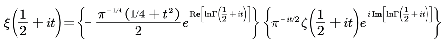
Evidently, the first factor on the right side of the above equation is always negative.
Therefore, studying the nontrivial zeros of the Riemann ξ(s) or ζ(s) function reduces to studying the zeros of the second factor, which in turn reduces to studying the sign changes of the second factor. For more details, refer to [1] [11].
Riemann’s own method of in-depth research, which was fortunately restored by Siegel in 1932 from the Riemann vestigial manuscript [1], is now well known as the Riemann-Siegel formula [11]. It is much more efficient than the Euler-Maclaurin formula, and was used to successfully calculate the first 3 approximate values of the imaginary parts of the nontrivial zeros on the critical line [1, p.134~137/168 - Figure 1] [11] by hand.
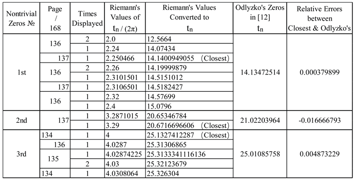
Remark: sometimes, in this paper, the values of the imaginary parts of the nontrivial zeros on the critical line are abbreviated as the zeros values, or zeros or tn.
As can be seen from Table 1, the first three best zeros with tn /2π rather than tn approximated by Riemann are very close to the current ones [12].
1.2.2 Based on the cumbersome and complex calculations for the nontrivial zeros on the critical line, and the fact that numerical calculations in Riemann's era were all done manually, this elementary calculation method was not well suited for calculating nontrivial zeros beyond. After determining the first three nontrivial zeros, Riemann turned to estimating the number of the nontrivial zeros on in a given range.
“He then goes on to say that the number of roots ρ whose imaginary parts lie between 0 and T is approximately” [3, p.18] [1]
where, N(T) denotes the number of the nontrivial zeros of Riemann ζ(s) function in the region 0 < Re(s) < 1, 0 < Im(s) < T. It also implies that N(T) approaches infinity as T → ∞. In 1905, the relationship above in equation [13] [5, p.17] was proven by von Mangoldt.
But it is still unknown whether this conclusion is also correct on line segment from 1/2 to 1/2+iT [3, p. 38]. In 1914, Hardy proved that there are infinitely many nontrivial zeros on the critical line [14]. With this and Section 1.2.1 above, the profile of the nontrivial zeros located on the critical line is basically clear—as long as one keeps calculating forever if necessary.
1.2.3 However, Riemann's formula for N(T) cannot determine whether there are the nontrivial zeros outside the critical line. This problem troubled Riemann since his paper and was also something he tried his best to solve but was not able to accomplish until his death. In such circumstances, “we can never know what led Riemann to say it was ‘probable’ that the roots ρ all lie on the line Re(s) = 1/2” [3, p.164], but as such, the Riemann Hypothesis was born in his paper [2].
2. Notation and Preparation
2.1. Main Notations
RxF, RzF: the Riemann and Functions, respectively.
CL, CS: the Critical Line and Critical Strip, respectively.
: the constant using for the critical line and this paper.
: the imaginary unit.
: the ordinal numbers.
: the total numbers of within or .
: a finite quantity setting in the analysis.
: the ordinal numbers or the natural numbers.
: the total numbers of the nontrivial zeros of RzF on the line, .
: the total (Hardy) numbers of the nontrivial zeros [13] of RzF on the upper half of CL.
: the number of the nontrivial zeros of RzF in CL with .
: a complex variable or number on the whole Complex Plane.
: the imaginary part of the nontrivial zero of RzF on the line, .
: the imaginary part of the nontrivial zero of RzF on the upper half of CL.
: a limiting quantity for describing the value of the imaginary part of nontrivial zeros on CL in the analysis of the Riemann hypothesis. .
: the Euler- Mascheroni constant, .
: a very small positive quantity introduced to avoid errors and enhance amplification effects.
: the horizontal offset that deviates from the critical line; .
: a constant; the quantity of the reciprocal sum formula for all the nontrivial zeros of RzF.
: the quantity of the reciprocal sum formula for all the nontrivial zeros of RzF in .
the quantity of the reciprocal sum formula for all the nontrivial zeros of RzF in .
: the constant, the quantity of the product formula of RxF at .
: the nontrivial zeros of Riemann function.
: a nontrivial zero of Riemann function.
: a nontrivial zero of Riemann function on the critical line.
: a nontrivial zero of Riemann function within .
: a nontrivial zero of RzF on the line, within .
: a nontrivial zero of RzF on the line, within .
: The counting function of primes.
: the point Set denoted within the area, on the Complex Plan; The region, is named the Critical Strip.
: the point Set denoted on the line, , which is called the Critical Line.
: the point Set denoted in the critical strip other than the critical line; .
: the left part and the right part of split by the critical line; .
2.2. Preparation
Property 1. All nontrivial zeros of RzF and All (nontrivial) zeros of RxF are coincident.
Property 3. All nontrivial zeros of RzF or RxF only form in the complex number.
Theorem 1. There are infinitely many nontrivial zeros of RzF on the critical line [14].
Theorem 2. The weak relationship [5, p.20] between tn and n is stated as
(A) .
Thus, the mean gapping gn between tn+1 and tn is
(B) ,
which approaches 0 as n → ∞ [15].
These are two of corollaries of the Riemann-von Mangoldt formula (theorem) [13] [5, p.17]:
, with .
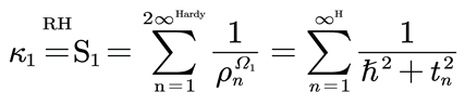
3. The Riemann Reciprocal Sum Formula
The reciprocal sum [1, p.72/168] of all nontrivial zeros of the Riemann or function can be expressed as
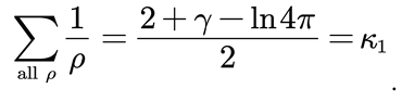
We notate this as the Riemann reciprocal sum constant and , separately.
Although this formula was not used and shown in his paper, Riemann had already derived it. What is even more surprising is that he accurately calculated this value as shown in Figure 2 below to 20 decimal places by hand. This may have helped him in his computations of the nontrivial zeros [3, p.67].
A comparison of Riemann's numerical value of and the value we obtained using MathCAD (accurate to within 10^-30) is as follows:

In the following section, Riemann's sufficiently accurate numerical value of will be employed as the criterion for our proof.
4. Proposition in This Paper and Its Proof
There should exist tetrad nontrivial zeros of the Riemann zeta function off the Critical Line.
Proof:
4.1. Theoretical Analysis
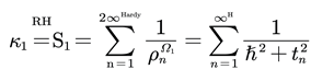
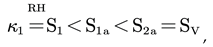
We denote that S1 and S2 are the reciprocal sums of the twin zeros and the tetrad zeros on and off the critical line, respectively. According to Property 3 and 4, the Riemann reciprocal sum formula, (6) can be separately adapted for Case 1 and Case 2 as

In other words, if the assumption of (7) or (8) holds, by Theorem 1 (Hardy Theorem [14]) and after introducing into S2, they can be respectively rewritten with the twin zeros and the tetrad zeros as
Or
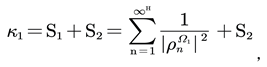
where,
Remark: when , (10) for Case 2 degenerates into (9); In the following derivation and proof process, we will not use S2, so there is no need to discuss it here in detail.
Splitting (9) into two parts, and then three parts, yields
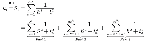
where, is a sufficiently large ordinal number (splitting point) which is reasonably selected from [12] to ensure that the reciprocal sum, Part 1 of the first twin zeros may become the principal term in (11); is an interval number of the first occurrence of a group for the twin zeros in (13) after .
Part 1 in (11) is a bounded series with random small periodic fluctuations, but has a monotonically increasing overall trend as increases.
Inserting δ, a very small positive quantity introduced to avoid errors and enhance amplification effects into Part 1 in (11), yields
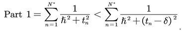
Using (12) and (13) and referring to (A) of Theorem 2 in Section 2, we can derive the following inequalities:
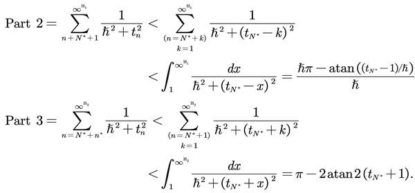
Remark: by Theorem 1 in Section 2, either both and are infinite, or one of them is finite and another is infinite. Based on (B) of Theorem 2 and the data from [12], we can make sure that . Even if is finite, replacing it with infinity does not affect the validity of Part 3 above. Therefore, in the above derivation, may be chosen.
We now set the sum of the first-level amplification effects in Part 1, 2 and 3 above as
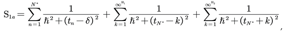
hence,
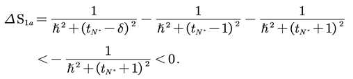
This means that as increases, S1a is a bounded sum with random small periodic and small fluctuations, and it has a monotonically DECREASING overall trend. This is also true for S2a.
The lower bound (which exists) of S1 will not be discussed because it appears unnecessary for the next objective of our numerical calculating verification.
Combining (11), Part 1, Part 2 and Part 3 above, we attain
where,
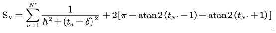
This shows that S2a (= SV) is the result of S1 being numerically enlarged— from a single numerical amplification by Part 1 and double numerical amplifications by Part 2 and Part 3.
4.2. Numerical Verification
Nowadays, although it is relatively easy to obtain nontrivial zeros on the critical line with the help of computers, it is impossible for humans to find an infinite number of zeros, such as Theorem 1 proven by Hardy. Fortunately, there are now a finite number of nontrivial zero values [12] on CL for free selection.
Selecting δ =1.1*10^-8, adopting Odlyzko's Tables of Zeros of the Riemann zeta function [12] and making use of WPS Office Sheet and MS Office Excel, the representative calculating results for SV are listed as follows:
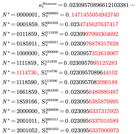
The above calculated values verify that S2a = SV, the reciprocal sums of all twin zeros after two numerical amplifications, is a bounded sum with random small periodic and small fluctuations but having a monotonically DECREASING overall trend as we have proved (15) before.
After the keen point, appears, the values of SV with double numerical amplifications are less than , and are ‘monotonically’ decreasing. Therefore, now we naturally have
Comparing (18) with (16) or (7), would yield a contradiction, because we assume earlier that all the nontrivial zeros of the Riemann zeta function are on the critical line. In other words, (8) is valid only when the Tetrad nontrivial zeros outside the critical line exist, and S2 in (8) plays a compensating role.
Our proposition is proved.
5. Summary
(a) We conclude that Riemann Hypothesis should be false;
(b) S1 is probable between 0.023093 - 0.023095;
(c) The determination of the Riemann reciprocal sum constant, for all nontrivial zeros may have been one of the key factors motivating the Riemann Hypothesis;
(d) Other analytical formulas for the reciprocal sum [15,16] of the nontrivial zeros for the Riemann zeta function can also be used to verify and prove our proposition by our method in this paper.
Conflicts of Interest
The authors declare no conflicts of interest.
References
- B. Riemann, Cod. Ms. B. Riemann 3 http://resolver.sub.uni-goettingen.de/purl?DE-611-HS-3226542.
- B. Riemann, Über die Anzahl der Primzahlen unter einer gegebenen Grösse. Monats berichte der Berliner Akademie, 671-680, November 1859. On The Number Of Primes Less Than A Given Magnitude, English translation by H. M. Edwards in [3], 1974.
- H. M. Edwards, Riemann’s Zeta Function. Dover Publications- New York, 1974.
- E. C. Titchmarsh, The Theory of the Riemann Zeta-Function. Oxford University Clarendon) Press, Oxford, London and New York, 1951; Second Ed. (Revised by D.R. Heath- Brown), 1986.
- J. Hadamard, Étude sur lespropriétés des fonctions entières et en particulier d’une function considérée par Riemann J. Math. Pures Appl. [4] 9, 171-215, 1893.
- J. Hadamard: Sur la distribution des zéros de la fonction ζ(s) et ses consequences arithmétiques. Bulletin de la S. M. F., tome 24, p.199-220, 1896.
- C.-J. De Vallée Poussin, Recherches analytiques sur la théorie des nombres premiers. Ann. Soc. scient. Bruxelles 20, p. 183-256,1896.
- J.P. Gram, Note sur les z´eros de la fonction ζ(s) de Riemann, Acta Mathematica, 27: .
- 289-304, 1903.
- C. L. Siegel, Über Riemanns Nachlass zur analytischen Zahlentheorie. Quellen und Studien zur Geschichte der Math. Astr. Phys., 2:45–80, 1932.
- A. Odlyzko, "Tables of Zeros of the Riemann Zeta Function" http://www.dtc.umn.edu/~odlyzko/zeta_tables/.
- H. von Mangoldt, Zu Riemann’s Abhandlung ‘Ueber die Anzahl der Primzahlen unter einer gegebenen Grösse’. J. Reine Angew. Math. 114,255-305, 1895.
- G. H. Hardy, Sur les zéros de la fonction ζ(s) de Riemann. C. R. Acad. Sci. Paris 158: p. 1012-1014, 1914.
- Wolfram MathWorld. https://mathworld.net.cn/Riemann-vonMangoldtFormula.htm.
- Wolfram MathWorld. https://mathworld.wolfram.com/RiemannZetaFunctionZeros.html.
Figure 1.
Riemann's approximate values of the first three nontrivial zeros on CL [1].
Figure 1.
Riemann's approximate values of the first three nontrivial zeros on CL [1].
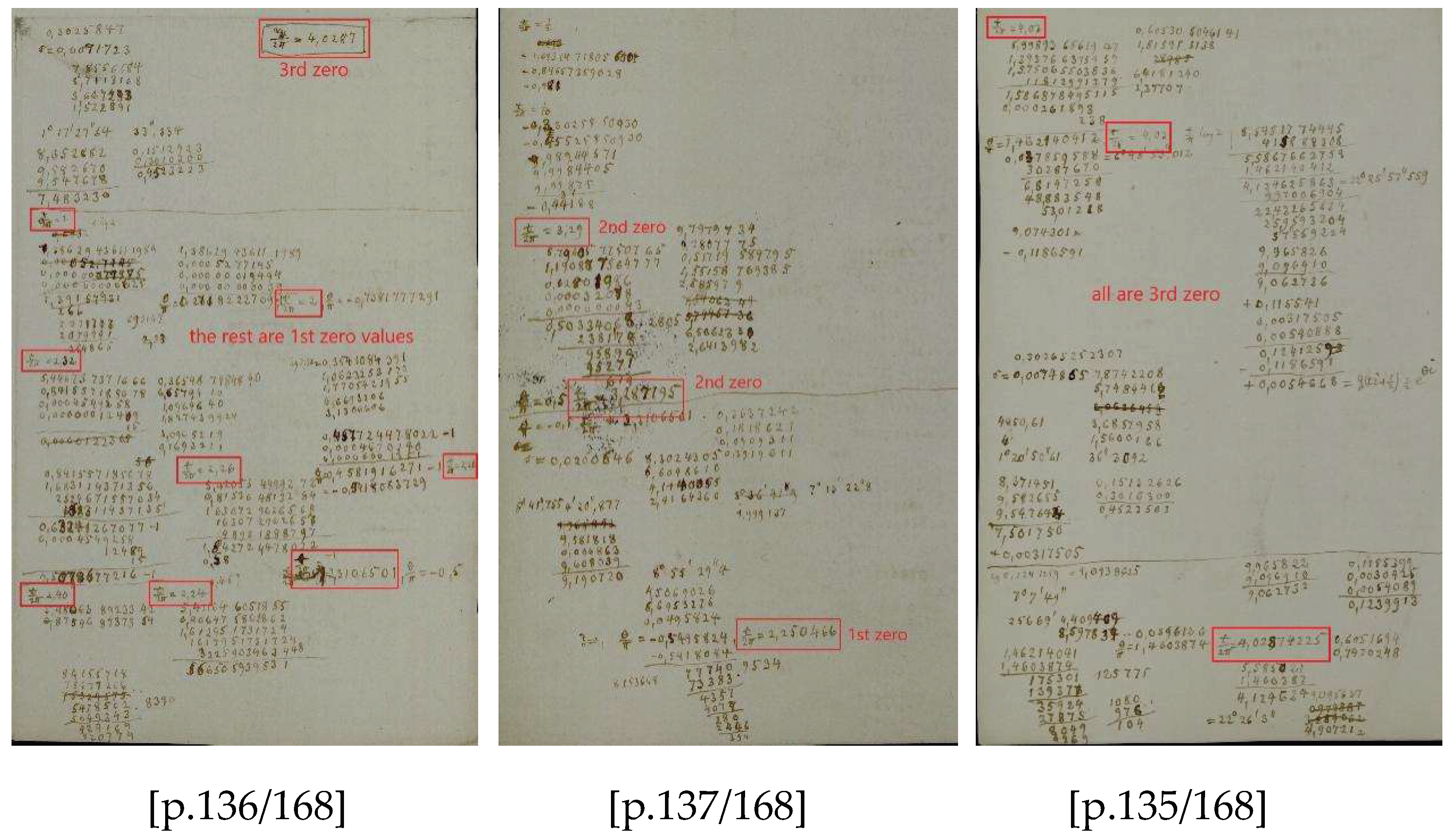
Figure 2.
Riemann's numerical value of the reciprocal sum formula [1, p.72/168].
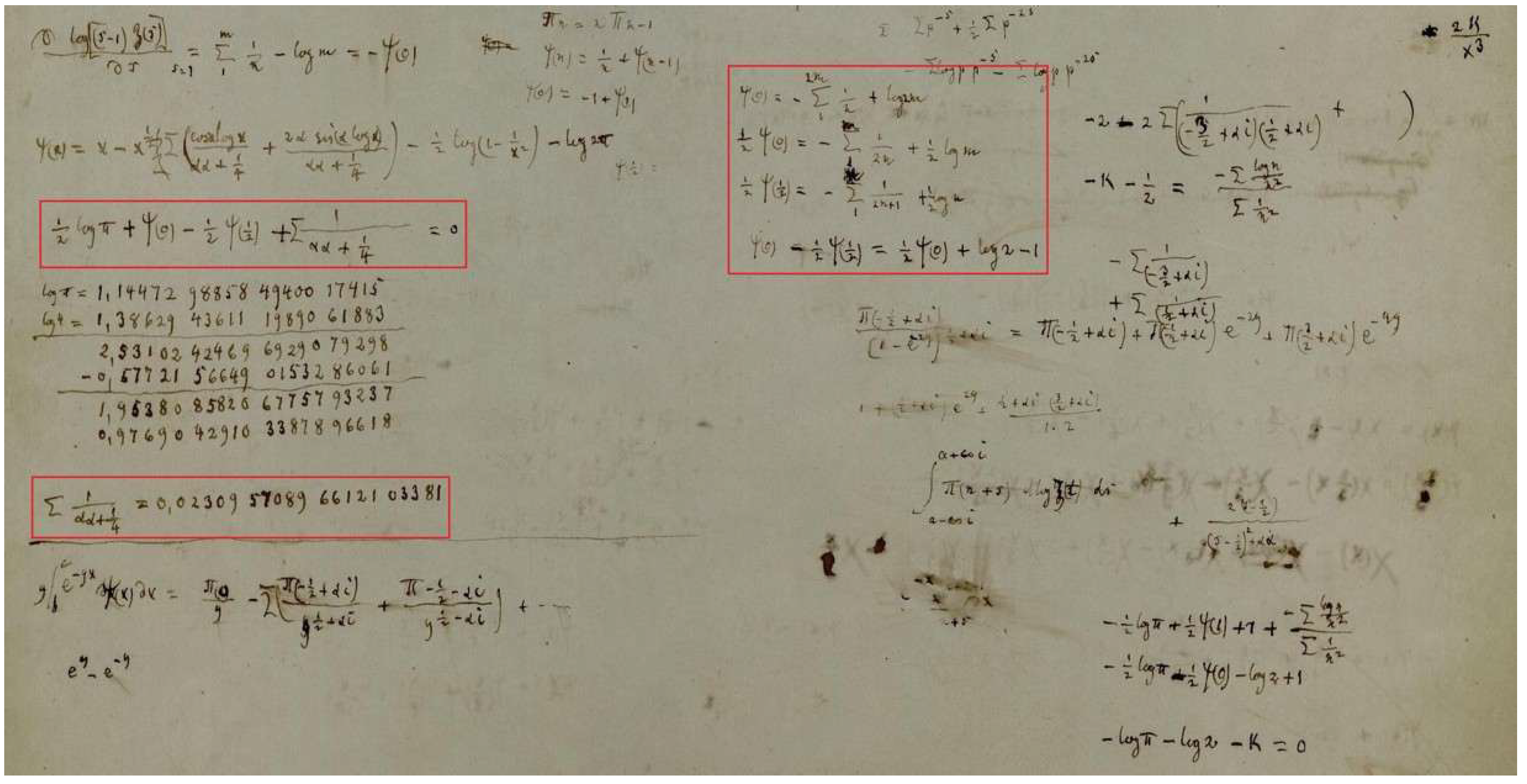

Table 1.
Riemann's Values of in [1].
Table 1.
Riemann's Values of in [1].
Disclaimer/Publisher’s Note: The statements, opinions and data contained in all publications are solely those of the individual author(s) and contributor(s) and not of MDPI and/or the editor(s). MDPI and/or the editor(s) disclaim responsibility for any injury to people or property resulting from any ideas, methods, instructions or products referred to in the content. |
© 2026 by the authors. Licensee MDPI, Basel, Switzerland. This article is an open access article distributed under the terms and conditions of the Creative Commons Attribution (CC BY) license.
Copyright: This open access article is published under a Creative Commons CC BY 4.0 license, which permit the free download, distribution, and reuse, provided that the author and preprint are cited in any reuse.


