Submitted:
15 January 2026
Posted:
16 January 2026
You are already at the latest version
Abstract
Convolutional neural networks are increasingly used for photovoltaic fault recognition from RGB imagery, yet high benchmark accuracy can mask shortcut learning induced by heterogeneous backgrounds, viewpoints and class imbalance. Using the Kaggle "PV Panel Defect Dataset" dataset, we compare five architectures (Baseline CNN, VGG16, ResNet50, InceptionV3 and EfficientNetB0) through a complementary explainability pipeline: LIME superpixel surrogates (with kernel-weighted R2 fidelity), occlusion sensitivity (functional relevance under localized masking) and Integrated Gradients (IG) validated by deletion-insertion curves. To reduce reliance on subjective saliency inspection, we quantify localization and concentration using IoU@Top10% against consistent proxy defect masks, Shannon entropy and Hoyer sparsity, and we summarize IG faithfulness with a Faithfulness Gap (AUC_insertion - AUC_deletion) and an accuracy-faithfulness consistency score at class level. ResNet50 attains the best predictive performance (82.3% accuracy), while EfficientNetB0 provides the strongest overall evidence faithfulness (mean Faithfulness Gap ~ 0.019) and stable, panel-centered attributions. InceptionV3 frequently yields diffuse relevance, and VGG16 produces highly concentrated but occasionally brittle hotspots. Bird-drop and Snow-covered show the most consistent alignment between accuracy and faithful evidence, whereas Clean and the two damage classes remain vulnerable to context cues (e.g., borders and background textures). The results support integrating quantitative explainability diagnostics into PV model selection and dataset curation to mitigate shortcuts and improve trustworthiness in vision-based PV monitoring.
Keywords:
explainable AI
; shortcut learning
; transfer learning
; photovoltaic panel
; fault detection
1. Introduction
Deep learning has transformed computer vision, with convolutional neural networks (CNNs) achieving state-of-the-art performance in image classification and related tasks. Architectures such as VGG, ResNet, Inception, and EfficientNet have shown remarkable ability to automatically learn hierarchical visual features, enabling applications from medical imaging to industrial monitoring.
Explainable artificial intelligence (XAI) has gained increasing attention as deep learning models achieve remarkable predictive accuracy while remaining largely opaque. Despite the proliferation of explainability techniques, no universal taxonomy or standardized classification currently exists to encompass all XAI methods. The literature reveals a wide range of frameworks that differ substantially in how explanations are categorized and applied. Cação et al. [1] proposed a unified classification integrating practical applicability and industrial relevance, while Tanzib Hosain et al. [2] highlighted the growing deployment of XAI in domains such as healthcare, finance, autonomous vehicles, and energy management.
1.1. XAI in Industry 4.0 and Energy Management
In the context of Industry 4.0, several XAI-integrated deep learning models have been developed for predictive maintenance and process optimization. Oyekanlu [3] designed an LSTM–RNN-based explainable framework for forecasting energy consumption in industrial IoT systems. Christou et al. [4] applied the Qarma family of algorithms to estimate the Remaining Useful Life (RUL) of machinery, while Sun et al. [5] proposed a CNN-based fault diagnosis model enhanced with Class Activation Maps (CAMs) for visual localization of damaged components without additional sensors. Serradilla et al. [6] employed Random Forests combined with LIME and ELI5 to improve the interpretability of machine health predictions.
In the energy/power sector, XAI has primarily been used for forecasting tasks. Kim et al. [7] introduced an architecture consisting of a projector and predictor, analogous to an encoder–decoder structure, both implemented with LSTM units to capture temporal dependencies in energy demand data. The projector compresses historical demand into a latent representation, while the predictor generates future demand, enabling end-to-end learning of the latent state. Such models enhance interpretability at the temporal level but remain limited to time-series data rather than image-based diagnostics.
1.2. XAI and Deep Learning for Photovoltaic Fault Detection
While forecasting dominates XAI research in energy systems, fault detection and diagnosis in renewable energy, particularly photovoltaics (PV), has become increasingly important. PV installations exhibit heterogeneous fault signatures, including cracks, discoloration, hotspots, and partial shading, which are difficult to detect through electrical parameters alone. Machine learning and computer vision techniques have therefore emerged as promising tools for automated visual fault analysis.
Awedat et al. [8] enhanced the U-Net architecture by incorporating residual blocks, atrous spatial pyramid pooling (ASPP), and attention mechanisms, significantly reducing false positives in segmentation-based PV fault detection. Sairam et al. [9] proposed an explainable three-component diagnostic framework combining a physical irradiance model, XGBoost classification, and XAI-based interpretability for each fault instance. Rico Espinosa et al. [10] introduced a CNN-based two-stage pipeline coupling semantic segmentation for panel localization with a classification network distinguishing breakage, shadows, dust, and no-fault conditions. Despite the small dataset, their method achieved reliable detection with approximately 70% accuracy, illustrating the feasibility of vision-based PV monitoring.
Performance degradation in PV modules arises from both intrinsic faults – such as delamination, cell cracks, or interconnection failures – and extrinsic soiling, including dust, bird droppings, snow, and industrial particulates. These factors reduce irradiance capture, induce thermal gradients, and accelerate local degradation. Traditional inspection methods (infrared thermography, electroluminescence, I-V tracing) remain accurate but are expensive and not scalable for large arrays. Vision-based machine learning offers a low-cost and scalable alternative capable of identifying both fault and soiling patterns in RGB imagery. Wan et al. [11] provided a comprehensive review of dust deposition mechanisms and monitoring approaches, covering both sensor-based and AI-driven systems. Restrepo-Cuestas et al. [12] presented an experimental dataset combining electrical parameters and thermographic imaging under various fault conditions, demonstrating significant power losses due to cracking and shading.
From the perspective of real-time fault recognition and on-device feasibility, Ling et al. [13] addressed recognition and real-time limitations in intelligent PV cleaning robots by improving YOLOv9t with three major innovations: integration of AOD-Net for dehazing, Spatial–Depth Conversion Convolution (SPD–Conv) to reduce computational cost, and an Inverted Residual Mobile Block–Efficient Multi-Scale Attention (iRMB–EMA) mechanism to improve robustness. Their approach increased mAP by 5.83% and reduced model size by 18.21% relative to baselines. Collectively, these studies confirm the potential of deep learning for PV fault analysis but also underscore a key limitation, which is the opacity of CNNs and their reliance on dataset-specific context rather than intrinsic fault cues.
1.3. From Photovoltaic Faults to General Issues in CNN Explainability
Although CNN-based models show promising performance, they often behave as black boxes whose decision-making criteria are not transparent. Trained on heterogeneous datasets, such models are prone to spurious correlations. Such shortcuts yield high apparent accuracy during validation but undermine robustness in unseen conditions. Incorporating XAI methods (e.g., LIME, Grad-CAM, and occlusion analysis) is therefore critical to verify that model predictions correspond to physically meaningful fault regions.
Importantly, this issue is not confined to PV analysis but reflects a broader challenge in computer vision. CNNs are known to rely on contextual features rather than intrinsic object representations, a behavior extensively documented in the literature. Beery et al. [15] and Torralba and Efros [16] demonstrated that classifiers often exploit background regularities – such as animals with their natural habitats – to achieve deceptively high accuracy. Geirhos et al. [17] characterized this as shortcut learning, where networks follow the path of least resistance in optimization, leveraging superficial correlations instead of semantic understanding. Lapuschkin et al. [18] further revealed that benchmark models can base their decisions on annotation artifacts, a behavior termed “Clever Hans,” which obscures the true reasoning process.
This problem extends across domains such as medical imaging, autonomous driving, and industrial monitoring. Rajpurkar et al. [19] showed that chest X-ray classifiers may depend on hospital-specific markers rather than pathologic features, while Zhang et al. [20] and others have documented similar vulnerabilities in safety-critical perception systems. These findings collectively highlight the necessity of integrating XAI not merely as a visualization tool but as a diagnostic framework for detecting biases and validating model reasoning. Techniques such as saliency mapping, class activation mapping, perturbation analysis, and surrogate modeling are increasingly used to expose hidden dependencies and to align model attributions with semantically meaningful evidence (Samek et al. [21]; Montavon et al. [22]).
In summary, the literature reveals that explainability is indispensable for ensuring the reliability of deep learning in both specialized domains such as PV fault detection and more general computer vision applications. The persistent problem of shortcut learning and contextual bias motivates the methodological framework adopted in this study, which combines multiple XAI techniques to analyze how CNNs form and justify their predictions.
1.4. Significance and Contribution of the Present Work
The present work contributes to the field of explainable deep learning by systematically analyzing the interpretability of CNN-based photovoltaic fault classification using complementary XAI techniques. While prior studies have focused primarily on improving accuracy or segmentation performance, few have examined why models succeed or fail when exposed to heterogeneous PV imagery. By integrating LIME, occlusion sensitivity, and Integrated Gradients, this research provides a multi-perspective interpretability analysis that distinguishes between correlational, gradient-based, and causal attributions.
The study demonstrates how CNN architectures ranging from simple convolutional baselines to advanced pretrained models such as EfficientNet and Inception arrive at their decisions, highlighting the degree to which each relies on intrinsic fault regions versus contextual artifacts. The findings reveal recurrent patterns of shortcut learning similar to those observed in broader computer vision benchmarks, thereby linking the PV domain to general challenges in model robustness and trustworthiness.
Beyond methodological insights, this work sets the ground for an experimental framework for evaluating the faithfulness of visual explanations in small, imbalanced datasets. The approach not only quantifies the reliability of CNN predictions but also exposes potential dataset biases that can mislead conventional accuracy-based evaluations. In doing so, the study contributes to both the applied understanding of PV fault detection and the theoretical advancement of explainable AI, supporting the development of more transparent, generalizable, and trustworthy computer vision systems for industrial and energy applications.
1.5. Objectives of the Study
This study aims to systematically evaluate the interpretability and reliability of convolutional neural networks (CNNs) in the classification of photovoltaic (PV) panel faults through complementary explainability techniques. The specific objectives are: (i) To compare the explanatory behavior of multiple CNN architectures (Baseline CNN, ResNet50, InceptionV3, EfficientNetB0, and VGG16) across diverse PV fault classes; (ii) To integrate three complementary XAI approaches: LIME (surrogate modeling), occlusion sensitivity (perturbation-based causality), and Integrated Gradient, to obtain a multifaceted understanding of model reasoning, and (iii) To identify cases of spurious or context-driven correlations that inflate model accuracy but compromise robustness and generalization.
Through these objectives, the study bridges the methodological gap between conventional performance metrics and interpretability-driven evaluation, advancing the deployment of explainable computer vision in renewable energy systems.
2. Dataset, Preprocessing, and Explainability Framework
2.1. Dataset and Preprocessing
The experiments were conducted on the publicly available Kaggle dataset “PV Panel Defect Dataset”, which contains six classes: Clean, Dusty, Bird-drop, Electrical fault, Physical fault, and Snow-covered. A subset of 875 images was selected in this work, with a marked imbalance across classes, as shown in Figure 1. In particular, the Physical fault class contains only 70 images, while Dusty and Clean exceed 190 images each. Such imbalance can bias models towards majority classes and motivates the need for an explainability analysis that goes beyond conventional accuracy metrics. The dataset is highly heterogeneous. Images were collected from diverse online sources, resulting in large variations in resolution (ranging from ~100×100 to >1000×1000 pixels), aspect ratios, lighting conditions, and viewing angles. Some samples include cluttered backgrounds (soil patches, vegetation, clear sky), while others focus closely on the photovoltaic module surface. This heterogeneity introduces noise and increases the likelihood that deep networks will learn associative context features (e.g., soil patches as indicators of dust) rather than intrinsic object features. To ensure comparability, all images were resized to a fixed input size of 224×224 pixels (299×299 in case of InceptionV3) and converted to RGB color space. Pixel intensities were normalized to the [0,1] range by scaling each channel by 1/255. No additional color space conversions (e.g., HSV, grayscale) were employed in the baseline experiments to remain consistent with the pretrained models used (EfficientNetB0, InceptionV3, ResNet50, and VGG16), which expect RGB inputs.
For both the custom CNN baseline and transfer learning experiments, no data augmentation was applied. This deliberate choice allows a direct assessment of each model’s intrinsic ability to generalize under limited and heterogeneous data conditions, without introducing artificial variability. Given the relatively small dataset size and the uncontrolled diversity of the original images, spanning a wide range of lighting conditions, angles, and backgrounds, further augmentation could have introduced biases in the real statistical distribution of visual features. The absence of augmentation therefore ensures that model behavior, including any reliance on contextual artifacts, reflects genuine dataset characteristics rather than artifacts introduced during preprocessing. The dataset was partitioned into training and validation subsets with an 80/20 split, stratified by class to preserve the imbalance distribution. The number of images and the mean resolution per class are presented in Figure 1. While stratified 80/20 split approach provides a baseline estimate of model performance, it does not fully mitigate the imbalance problem. Therefore, the integration of explainability methods such as LIME becomes crucial: high reported accuracy may conceal the fact that models base their decisions on contextual or spurious features instead of the actual physical faults in the panels.
2.2. Architectural Framework of the Deep Learning Models
Five convolutional neural network (CNN) architectures were employed in this study: Baseline CNN, VGG16, ResNet50, InceptionV3, and EfficientNetB0. The structural overviews of the selected architectures are presented in Figure 2. The Baseline CNN, trained from scratch, consists of two convolutional layers followed by normalization, pooling, and fully connected stages, serving as a control for generalization under limited data. VGG16 represents an early deep architecture composed of uniform 3×3 convolutional blocks and max-pooling operations, forming a sequential and interpretable hierarchy. ResNet50 introduces residual connections that enable information flow across layers, mitigating gradient vanishing and improving feature reuse through bottleneck blocks. InceptionV3 employs a multi-branch design with parallel convolutions of varying receptive-field sizes, capturing both local and global patterns within the same layer depth. EfficientNetB0 exemplifies compound scaling, balancing network depth, width, and resolution through MBConv blocks optimized for efficiency. All pretrained models were truncated before their classification heads and extended with a Global Average Pooling (GAP) layer-an operation that averages each feature map spatially to a single representative value-followed by dense layers and dropout regularization. This standardized structure facilitates direct comparison of feature extraction behavior across architectures under identical training conditions.
Despite their structural differences, all CNNs share the same opacity in internal reasoning-making it difficult to determine whether predictions rely on genuine fault-related features or on spurious contextual cues such as background textures or lighting patterns. To address this, three complementary explainability techniques were applied-LIME, occlusion sensitivity, and Integrated Gradients-each providing a distinct perspective on the spatial and functional basis of model predictions. Together, these approaches enable a multi-faceted interpretation of CNN behavior, offering both visual and analytical insights into the decision mechanisms underlying PV fault classification.
2.3. Performance Metrics
The performance metrics for all architectures computed over the validation set are presented in Supplementary Material 1, Tables S1.1-S1.6. The quantitative evaluation highlights a clear performance gap between the baseline CNN and the transfer-learning architectures, with the former achieving only moderate accuracy (63.8%) and macro-F1 (0.618), indicative of limited class-wise generalization. In contrast, pretrained models substantially improve both metrics, with ResNet50 yielding the strongest overall performance (accuracy = 82.3%, macro-f1 = 0.825). While visually distinctive classes such as Snow-covered and Electrical damage are consistently detected with high recall across architectures, Physical damage remains the most challenging category, exhibiting persistently lower recall even for the best-performing model. The corresponding confusion patterns indicate that residual errors are dominated by misclassifications among visually and structurally similar fault types rather than confusion with the Clean class. These results provide an essential quantitative baseline for the subsequent analysis of occlusion-based explainability maps, where we investigate whether the spatial attribution patterns reflect these systematic strengths and failure modes. The baseline CNN exhibits pronounced class imbalance effects, with strong precision but low recall for certain fault types (e.g., Physical damage), resulting in substantial off-diagonal entries in the confusion matrix. Transfer-learning models markedly reduce these errors, achieving improved diagonal dominance, particularly for Electrical damage and Snow-covered samples. Nevertheless, consistent misclassification patterns persist across architectures for fault classes sharing similar texture and structural characteristics, confirming that remaining errors are systematic rather than random. These supplementary results substantiate the comparative performance claims made in the main text and serve as a quantitative reference point for interpreting the model-specific occlusion sensitivity and XAI visualizations discussed later throughout the paper.
3. Explainability Framework
3.1. LIME-Based Explainability for Image Classification Models
To provide local, instance-level interpretability for the five CNN architectures, we implemented an image-adapted LIME procedure based on superpixel-level perturbations and a kernel-weighted linear surrogate. For each test image, the RGB input is first resized to the model-specific resolution (224×224 for Baseline CNN/EfficientNetB0/ResNet50/VGG16 and 299×299 for InceptionV3) and preprocessed using the corresponding normalization pipeline. The image is then partitioned into perceptually coherent regions using Quickshift superpixels, (Vedaldi and Soato [23]), implemented using scikit-image (with the parameter , , ), and the resulting segment labels are relabeled to a contiguous index set . This superpixel formulation is motivated by both interpretability and perturbation realism: superpixels act as human-meaningful explanation units (capturing local edges, textures, and homogeneous PV-surface areas) and avoid pixel-wise masking artifacts that are difficult to interpret and can generate out-of-distribution inputs in heterogeneous outdoor scenes. Local neighborhoods are constructed by sampling binary activation vectors (with ), where each perturbation masks entire superpixels rather than individual pixels; masked regions are replaced with a per-image mean RGB baseline, yielding perturbed images that remain visually plausible compared with hard dropout. For each perturbed sample, we query the black-box, trained architecture, and record the probability of the predicted class of the unperturbed image (), i.e., . Perturbations are weighted by a locality kernel based on cosine distance to the all-superpixels-on reference : , and with . A Ridge regression surrogate (weighted by , ) is fitted to approximate the local mapping from superpixel inclusion to predicted-class probability; its coefficients provide a ranked attribution over superpixels, and we visualize the Top-3 positively contributing regions with consistent rank encoding (Red/Green/Blue) and a matched coefficient bar plot. Importantly, because superpixel explanations trade spatial precision for perturbation plausibility and locality, superpixel choice and segmentation granularity can influence the fitted surrogate; therefore, we report per-image kernel-weighted surrogate fidelity (, ) to avoid over-interpreting explanations when the local linear approximation is unstable.
3.1.1. Kernel-Weighted for LIME Surrogate Fidelity
Let denote the -th LIME perturbation vector over superpixels, and let be the corresponding perturbed image obtained by masking the inactive superpixels. For the class explained (typically the predicted class on the unperturbed image), we define the model response:
and the surrogate prediction:
where is the fitted linear surrogate (e.g., ridge/linear regression) trained with locality weights .
Distances are computed between each perturbation and the all-ones vector (i.e., the unmasked configuration), using cosine distance:
The kernel weight for perturbation with the index is given by:
where is the kernel width (in your runs, ).
We define the weighted mean:
and weighted SSE and SST:
The kernel-weighted coefficient of determination is calculated with:
Where is a small constant for numerical stability (the value was used). The values of range in the interval indicating that the linear surrogate accurately approximates the model’s local response over the neighborhood emphasized by the LIME kernel.
Weighted MSE
To quantify the reliability of LIME explanations beyond qualitative inspection, we report the kernel-weighted surrogate fidelity of the local linear model fitted to the LIME perturbation samples. Specifically, for each explained image we compute the weighted coefficient of determination (and the corresponding weighted MSE) between the architecture’s predicted-class probability on perturbed inputs and the surrogate’s predictions, using the same locality weights as the LIME kernel. Low values indicate locally non-linear decision behavior that is poorly captured by a linear surrogate; in such cases, coefficient-based superpixel attributions should be interpreted cautiously. Table 1 summarizes surrogate-fidelity statistics across architectures. Table 1 presents synthetically, for each architecture, both the central tendency and the tail behavior of LIME surrogate fit under the exact perturbation protocol used to generate explanations. Table 1 reports the following:
(i) , the number of explained validation images per model;(ii) (the mean value of ) and (the 10th set percentile), where is the kernel-weighted coefficient of determination between the architecture’s response on perturbations and the surrogate prediction , computed with the LIME locality weights (thus capturing fidelity in the local neighborhood emphasized by LIME);(iii) , the mean predicted-class probability on the unperturbed images, included to contextualize surrogate fidelity with respect to model confidence;(iv) , the mean number of superpixels produced by the chosen segmentation settings (quickshift), serving as a proxy for explanation granularity and complexity of the surrogate feature space;(v) , the fraction of a model’s instances falling below the global low-fidelity threshold (defined as the bottom decile of across all image model pairs), indicating how often LIME explanations for that architecture enter a regime where linear surrogates are unreliable; and(vi) the fraction of instances exceeding the global high-fragmentation threshold (top decile of ), indicating how frequently segmentation produces highly fragmented partitions that can destabilize coefficient-based attributions.
The Baseline CNN exhibits consistently high surrogate fidelity ( mean , 10th percentile ), indicating that its output varies approximately linearly under superpixel masking; however, it also shows the lowest average predicted-class confidence (), emphasizing that a faithful local surrogate does not necessarily imply strong or physically grounded evidence. At the other extreme, VGG16 yields the weakest surrogate fidelity ( mean , 10th percentile ) while maintaining high confidence (), revealing locally complex score–perturbation relationships where LIME’s linear approximation becomes unreliable despite confident predictions. EfficientNetB0 shows intermediate-to-good fidelity ( mean , 10th percentile ), whereas ResNet50 and InceptionV3 are lower ( means and , respectively). Notably, InceptionV3 produces a markedly larger number of superpixels on average (, versus for 224×224 models), reflecting a more fragmented interpretable partition that can increase explanation variance and dilute coefficient interpretability. A class-model worst-case inspection (Supplementary Material S2) further confirms that the lowest surrogate fits concentrate in visually diffuse regimes (e.g., Snow-Covered), with extreme cases such as VGG16 × Snow-Covered reaching at near-unit confidence, reinforcing that confidence and “visually clean” explanations alone are insufficient without surrogate-fidelity context.

Table 1.
LIME surrogate-fidelity summary.
| Architecture | ||||||
| VGG16 | 0.289 | 0.171 | 0.88 | 0.425 | 159 | 0 |
| ResNet50 | 0.4159 | 0.293 | 0.81 | 0.078 | 159 | 0 |
| InceptionV3 | 0.476 | 0.386 | 0.69 | 0 | 279 | 0.51 |
| EfficientNetB0 | 0.558 | 0.457 | 0.67 | 0 | 159 | 0 |
| Baseline_CNN | 0.915 | 0.853 | 0.60 | 0 | 159 | 0 |
To further characterize where LIME becomes unreliable, we performed a class–model worst-tail audit and provide the complete listings in Supplementary Material S2 (worst_cases_by_class_model.csv). For each architecture and each PV-fault class, we selected the six instances with the highest “badness” score (dominated by low kernel-weighted surrogate fidelity , and optionally amplified by low confidence or high superpixel fragmentation), thereby isolating regimes where the local linear surrogate is least able to approximate the model response under superpixel masking. The resulting worst-tail patterns are summarized by two compact heatmaps: Figure 3 reports the mean within the worst-tail subset for each class×model pair, while Figure 4 reports the corresponding minimum , highlighting the most extreme failure modes. These maps reveal that LIME fragility is not uniform across categories: visually diffuse and globally distributed phenomena (most notably Snow-Covered) concentrate the lowest-fidelity cases, and architecture-specific weaknesses emerge (e.g., VGG16 exhibits particularly low worst-tail for Snow-Covered despite high prediction confidence). By explicitly reporting both average and extreme surrogate-fidelity behavior in the worst-tail, we complement the global summary of Table 1 and provide a transparent, reproducible basis for selecting representative examples and for interpreting LIME coefficients cautiously in locally non-linear regimes.
The two all-sample heatmaps are provided in the Supplementary Material S3 (Figures S3.1 and S3.2) to document the global baseline of LIME surrogate fidelity across the entire validation set, thereby complementing the main-text worst-tail analysis (which is intentionally focused on failure modes) and enabling the distinction between typical behavior and tail-risk extremes. Taken together, the four heatmaps show a consistent hierarchy in LIME surrogate fidelity: Baseline CNN remains highly linear under masking (high mean and high minima), EfficientNetB0/InceptionV3 occupy a stable intermediate regime, whereas ResNet50 and especially VGG16 exhibit markedly lower fidelity with the strongest tail-risk (lowest minima), and this degradation concentrates in visually diffuse regimes such as Snow-Covered, confirming that LIME reliability is jointly driven by architecture and class-specific visual structure and motivating explicit reporting of both global and worst-tail surrogate-fit diagnostics.
Supplementary Material S4 (Zenodo, doi:10.5281/zenodo.18233689) provides the complete set of LIME visualization outputs for the full test set, preserved in the original class-wise folder structure. For each test image, four PNG files are included: (i) the resized original, (ii) the superpixel segmentation overlay, (iii) the LIME RGB overlay highlighting the top-3 ranked superpixels (red/green/blue), and (iv) a bar plot of the corresponding top-3 Ridge surrogate coefficients (with the model’s predicted label and probability reported in the plot title).
3.1.2. Selection Policy for Representative and Failure-Mode LIME Examples
For the LIME examples reported in the main manuscript, we adopted an explicit best–worst per architecture curation policy intended to showcase both representative explanatory behavior and “tail-risk” failure modes. For each architecture (Baseline CNN, EfficientNetB0, ResNet50, InceptionV3, VGG16), we selected exactly two test images using surrogate fidelity as the primary criterion. Fidelity was quantified by the kernel-weighted coefficient of determination , computed between (i) the black-box model’s predicted-class probability on the LIME perturbed samples and (ii) the corresponding predictions of the locally fitted Ridge surrogate, using LIME’s locality weights derived from the exponential kernel. The resulting curated set is summarized in Table 2, which documents for each selected case the architecture, extremal type (pick, BEST/WORST), the directory ground-truth label, surrogate fidelity () and weighted error (), as well as the model’s predicted label and confidence on the unperturbed image (Predicted, Prob) to provide decision-regime traceability.
Selection was performed within each architecture. The BEST example was defined as the case with the highest available , while preferentially restricting the search to robust operating conditions: whenever the required fields were available, we prioritized images for which the unperturbed prediction was high-confidence (e.g., ) and, when possible, correct (predicted label matches the ground truth), so that high-fidelity explanations are demonstrated under the intended regime of correct decisions. Conversely, the WORST example was defined as the case with the lowest available , with priority given to high-confidence cases when available, because low surrogate fidelity under high confidence is most diagnostic of LIME limitations – namely strong local nonlinearity of the classifier, sensitivity to superpixel segmentation, or instability of the local perturbation neighborhood. If a preferred subset was empty for a given architecture (i.e., no candidates satisfied the confidence and/or correctness preference), we applied a deterministic fallback and selected the global maximum (BEST) or global minimum (WORST) among all test images available for that architecture.
To make the extremal nature of each choice auditable, Table 2 additionally reports r2_rank (the rank of the selected case when all test samples for that architecture are sorted by in descending order) and r2_p, the percentile of , indicating whether the selected sample is a strict extreme or a near-extreme due to preference constraints. Thumbnail previews of the selected BEST/WORST exemplars, together with the corresponding Top-3 LIME superpixels, are provided in Supplementary Material 5 for visual traceability.
Table 2.
Best–worst LIME exemplar set per architecture (surrogate-fidelity curation).
| Model | Pick | Ground Truth | Prob | Predicted | r2_rank | r2_p | ||
| 1 | B | Clean | 0.974 | 1.01E-04 | 0.812 | Clean | 2 | 0.993 |
| W | Snow-Covered | 0.772 | 8.06E-04 | 0.811 | Snow-Covered | 139 | 0.014 | |
| 2 | B | Clean | 0.727 | 1.28E-03 | 0.909 | Clean | 1 | 1.000 |
| W | Snow-Covered | 0.427 | 6.40E-04 | 0.944 | Snow-Covered | 134 | 0.050 | |
| 3 | B | Snow-Covered | 0.623 | 7.10E-03 | 0.862 | Snow-Covered | 3 | 0.986 |
| W | Bird-drop | 0.366 | 9.33E-03 | 0.935 | Bird-drop | 135 | 0.043 | |
| 4 | B | Clean | 0.620 | 1.04E-02 | 0.858 | Clean | 3 | 0.986 |
| W | Snow-Covered | 0.185 | 4.75E-04 | 1.000 | Snow-Covered | 140 | 0.007 | |
| 5 | B | Bird-drop | 0.492 | 6.27E-02 | 0.956 | Bird-drop | 1 | 1.000 |
| W | Snow-Covered | 0.101 | 1.14E-06 | 1.000 | Snow-Covered | 141 | 0.000 |
1 – Baseline CNN; 2 – EfficientNetB0; 3 – ResNet50; 4 – InceptionV3; 5 – VGG16; B – Best case; W – Worst case.
3.2. Functional Interpretability Through Occlusion Sensitivity
3.2.1. Occlusion Sensitivity Maps
Occlusion sensitivity analysis (Figure 5) provides an intervention-based view of model evidence by quantifying the change in predicted-class confidence when local image patches are masked. Across the representative occlusion maps in Figure 5, the architectures exhibit distinct “evidence utilization” modes that are class dependent. For context-rich scenes (Dust and the second Bird-drop exemplar), the Baseline CNN frequently assigns functional relevance to peripheral structures and background terrain, indicating a context-driven decision pathway consistent with shortcut learning under dataset heterogeneity. EfficientNetB0, in contrast, more consistently anchors relevance on the PV surface and along physically plausible transitions (e.g., soiling gradients or snow boundaries), yielding a balanced pattern that remains informative both for diffuse phenomena (Dust, Snow-covered) and compact faults (Bird-drop). ResNet50 often produces multi-island relevance distributions, suggesting partial structural awareness but weaker selectivity. VGG16 tends to generate highly peaked maps (few intense hotspots), which aligns with its high sparsity/low entropy profile, but also implies vulnerability to point-cue reliance when the hotspot does not coincide with the true defect. Finally, Inceptio”V3 f’equently yields spatially diffuse heatmaps - consistent with high entropy and near-zero sparsity - so that coarse overlap with defect masks may occur (notably for large-area phenomena such as Snow-covered) without providing fine-grained localization. Overall, Figure 5 reinforces that interpretability cannot be inferred from accuracy alone: models may achieve correct predictions while relying on markedly different – and sometimes non-physical – evidence sources.
3.2.2. Occlusion Sensitivity Quantitative Analysis
To complement the qualitative inspection of LIME visualizations and to establish a more objective basis for evaluating model interpretability, we developed a quantitative occlusion sensitivity pipeline implemented in TensorFlow and OpenCV. This procedure systematically perturbs the input image by masking localized square patches and records the resulting variation in prediction confidence. The resulting response maps quantify the causal influence of each spatial region on the model’s decision, enabling reproducible comparison across architectures and damage categories. In contrast to gradient-based techniques, occlusion sensitivity directly probes the decision surface of the trained model, thereby providing a measure of functional relevance rather than correlation.
Occlusion sensitivity assigns each spatial region a functional influence score by measuring the change in predicted-class confidence under localized interventions. For each image , we define the reference class as the model’s top-1 prediction on the unoccluded input and compute, for each patch location , the log-probability drop with , where is obtained by replacing the patch with the per-image mean RGB value. Negative impacts (occlusion increasing confidence) are clamped to zero to retain evidence-decreasing contributions. The resulting grid map is upsampled bicubically and resized to a common resolution for cross-architecture comparability, then max-normalized to . We quantify (i) localization via IoU@Top10%, computed between the top 10% most influential pixels (percentile-thresholded) and a consistently generated automatic proxy mask, (ii) dispersion via Shannon entropy computed on the normalized relevance mass , and (iii) compactness via Hoyer sparsity based on the ratio of the vectorized map. These complementary measures separate where evidence is concentrated (IoU) from how it is distributed (entropy/sparsity), and are interpreted alongside qualitative overlays (Figure 5). Formal definitions of the occlusion impact map and quantitative metrics (IoU@Top10%, entropy, Hoyer sparsity), including numerical-stability constants and units, are provided in Supplementary Material S6.
Occlusion metrics were computed on the full validation set under identical occlusion hyperparameters for all architectures; the evaluation is balanced across models and classes (equal number of images per class–model pair). Table 3 summarizes the quantitative occlusion-sensitivity metrics aggregated over the validation set, while Figure 5 provides representative qualitative examples. Overall, VGG16 exhibits the strongest functional localization, achieving the highest IoU@Top10% (0.172 ± 0.145), the lowest entropy (8.391 ± 2.700), and the highest Hoyer sparsity (0.520 ± 0.277), indicating comparatively compact and mask-aligned relevance distributions under perturbation. EfficientNetB0 shows similarly high sparsity (0.449 ± 0.146) but lower overlap with the defect masks (IoU@Top10% = 0.096 ± 0.051), suggesting that its relevance is often concentrated yet not consistently aligned with the automatically derived fault regions. ResNet50 attains intermediate IoU (0.130 ± 0.114) but markedly lower sparsity (0.183 ± 0.252), consistent with broader relevance spread across the image. InceptionV3 yields the weakest localization signal, with near-zero sparsity (0.013 ± 0.094) and the highest entropy (10.321 ± 2.209), consistent with the visually diffuse occlusion maps observed in Figure 5. Taken together, these results indicate that architectural differences in functional relevance are measurable at dataset scale, and that high-confidence predictions (PredProb) do not necessarily imply spatially faithful or mask-aligned evidence.
3.2.3. Model-Level Interpretability Metrics
The updated model-level occlusion metrics (Figure 6, Figure 7 and Figure 8 with the error bars denoting standard deviation across N=141 test images) reveal marked differences in how architectures distribute functional relevance, and they also clarify that concentration and localization are not interchangeable. VGG16 exhibits the lowest mean entropy (8.391 ± 2.700) and the highest Hoyer sparsity (0.520 ± 0.277), indicating highly concentrated occlusion maps. Consistently, it also achieves the highest IoU@Top10% (0.172 ± 0.145), i.e., the top 10% most influential pixels overlap most with the automatically generated defect masks. However, this “best” IoU–sparsity combination should be interpreted cautiously: strong concentration can inflate overlap when masks are compact or imperfect, and qualitative inspections (occlusion/LIME) still show that VGG16 may lock onto small, high-contrast hotspots that are not necessarily the true fault evidence. In contrast, InceptionV3 yields the highest entropy (10.321 ± 2.209) and near-zero sparsity (0.013 ± 0.094), confirming diffuse relevance and an over-smoothing tendency, while still producing a mid-range IoU@Top10% (0.111 ± 0.064), consistent with coarse but weakly localized alignment. ResNet50 attains the second-highest IoU@Top10% (0.130 ± 0.114) with moderate entropy (9.321 ± 3.157) but low sparsity (0.183 ± 0.252), suggesting broader evidence integration rather than compact localization. EfficientNetB0 shows a more stable profile - moderate IoU@Top10% (0.096 ± 0.051), relatively low entropy (9.760 ± 0.555), and high sparsity (0.449 ± 0.146) - which aligns with the interpretation of a balanced, consistently focused attention mechanism. Finally, the Baseline CNN yields the lowest IoU@Top10% (0.083 ± 0.030) alongside intermediate sparsity and entropy, reflecting weaker and less reliable localization. Overall, these results emphasize that high IoU can coexist with low faithfulness (as we will show in the next section by IG-based metrics), and that robust interpretability requires jointly considering localization, concentration, and faithfulness rather than any single metric in isolation.
3.2.4. Per-Class Interpretability Analysis
Figure 9, Figure 10 and Figure 11 summarize how occlusion-derived interpretability metrics vary across defect categories and architectures, revealing that the same model can exhibit significantly different explanation behavior depending on the visual structure of the class. Importantly, these class-wise patterns refine the model-level trends discussed in Section 3.2.3: high localization (IoU@Top10%) can coincide with either concentrated or distributed saliency, and concentration (high Hoyer / low entropy) should not be conflated with semantic correctness. The qualitative overlays in Figure 5 provide the necessary visual anchor for interpreting these metrics, showing that architectures differ not only in “how much” relevance they assign, but also in where and how coherently relevance is distributed over the PV surface versus contextual background.
From a localization standpoint (Figure 9), VGG16 achieves the highest IoU@Top10% in five out of six classes (Bird-drop, Clean, Dusty, Electrical-damage, and Physical-Damage), indicating that its most influential occluded regions frequently overlap the automatically derived defect masks. However, this consistent “best” overlap must be read together with Figure 9, Figure 10 and Figure 11 and with Figure 5: VGG16 also exhibits strongly concentrated maps (high Hoyer sparsity across most classes) and low entropy relative to other architectures, implying that overlap is often driven by a small number of high-impact hotspots. This aligns with the qualitative behavior in Figure 5, where VGG16 tends to lock onto compact, high-contrast regions. Such concentration can be advantageous when the defect truly forms compact salient structures (e.g., localized bird-drop patterns or sharp electrical damage cues), but it also raises the risk of over-reliance on spurious, high-contrast artifacts, i.e., high overlap does not necessarily guarantee physically meaningful evidence.
The concentration–diffusion separation becomes explicit in Figure 10 (Hoyer sparsity) and Figure 11 (entropy). InceptionV3 systematically yields near-zero sparsity across all classes and the highest entropy, confirming highly dispersed relevance distributions that are weakly localized – again matching the almost uniform heatmaps observed in Figure 5. EfficientNetB0 shows stable, moderate-to-high sparsity across classes, often ranking second after VGG16, while simultaneously maintaining comparatively moderate entropy (Figure 11). This combination supports the qualitative impression from Figure 5 that EfficientNetB0 tends to anchor evidence on the PV surface and preserve coherent relevance transitions rather than spreading attribution over the whole scene. ResNet50 occupies an intermediate regime: its sparsity is lower than EfficientNetB0 and substantially below VGG16, while entropy is also typically moderate, consistent with the “multi-island” attribution patterns observed in Figure 5 – suggesting evidence integration from multiple spatial cues rather than a single hotspot. The Baseline CNN generally remains less distinctive than the pretrained backbones, showing intermediate sparsity and relatively high entropy in several classes, consistent with a greater sensitivity to context and background structures.
Finally, the class dependency of these metrics is particularly informative for understanding where localization is intrinsically harder. Snow-Covered class consistently exhibits the weakest IoU@Top10% across architectures (Figure 9), reflecting the fact that snow coverage often reduces contrast and introduces large, diffuse regions with soft boundaries, making precise localization difficult for occlusion-based maps. In this regime, models that produce compact hotspots (e.g., VGG16) may fail to match extended masks despite strong concentration, whereas a diffuse model (InceptionV3) can obtain relatively better overlap simply by distributing relevance broadly over the scene. Taken together, Figure 9, Figure 10 and Figure 11 and the qualitative evidence of Figure 5 support a key methodological point: interpretability assessment should be multi-metric - localization (IoU), concentration (Hoyer), and dispersion (entropy) capture complementary properties, and only their joint interpretation can distinguish “focused but potentially brittle” explanations (e.g., VGG16) from “diffuse and weakly localized” explanations (InceptionV3) and more balanced behaviors (EfficientNetB0/ResNet50).
3.3. Integrated Gradients
3.3.1. General Theory of Integrated Gradients
To complement the perturbation-based occlusion sensitivity analysis, Integrated Gradients (IG) was employed to derive gradient-integrated attribution maps that capture the cumulative influence of each pixel on the predicted class. Unlike occlusion sensitivity, which measures confidence variation under explicit masking, IG integrates the model’s gradient response along a continuous interpolation path from a neutral baseline to the actual image, providing a smooth and analytically grounded estimate of functional relevance.
Integrated Gradients is an attribution method that explains the prediction of a model by measuring how changes in each input pixel (or feature) affect the output along a continuous path from a baseline input to the actual input.
For a model , an input and a baseline the IG attribution for input dimension is defined as:
In practice, this path integral is approximated via a Riemann sum over a finite interpolation steps :
The resulting attribution scores form a pixel-wise relevance map that approximately satisfies the completeness property, i.e. allowing the prediction to be decomposed into a sum of feature contributions.
For the qualitative interpretability analysis, Integrated Gradients was computed for all five trained classifiers (Baseline CNN, EfficientNetB0, ResNet50, InceptionV3, VGG16). For each model and class, two correctly classified test images were selected, and IG attributions were obtained along a straight-line path from a zero-valued (black) baseline image to the actual input, using 50 interpolation steps. At each step, gradients were taken with respect to the output score of the predicted class, and the resulting attributions were averaged over the interpolation path to obtain a pixel-wise attribution map. The IG maps were then converted to relevance heatmaps by taking the absolute values, averaging across color channels, and applying min - max normalization to the [0,1] range, after which they were overlaid on the original RGB images using a fixed blending factor to facilitate visual inspection.
3.3.2. Faithfulness of IG Explanations (Deletion–Insertion)
Beyond visual inspection, the faithfulness of IG explanations was quantified using the Deletion–Insertion framework. For each architecture, we computed the area under the confidence–perturbation curves (AUC) for progressive pixel removal (Deletion) and re-insertion (Insertion), and defined the Faithfulness Gap as:
Positive values of indicate that the confidence of the model decreases when highly attributed pixels are removed and recovers when they are reintroduced, reflecting a causal rather than merely correlative relationship between the explanation and the decision. Table 4 summarizes the faithfulness metrics and the faithfulness gap.
Figure 12 shows a consistent global ranking in terms of the mean faithfulness gap Δ over the evaluation set (N = 141). EfficientNetB0 yields the largest mean gap ( = 0.0192), followed by ResNet50 ( = 0.0153) and the Baseline CNN ( = 0.0106), whereas VGG16 ( = 0.0077) and especially InceptionV3 ( = 0.0049) show weaker separation between insertion and deletion curves. Notably, the Baseline CNN combines the lowest deletion AUC (rapid confidence degradation under removal) with limited recovery under insertion, producing only an intermediate Δ.
The global comparison presented in Figure 12 shows the mean faithfulness gap aggregated over all six classes for each architecture. EfficientNetB0 achieves the highest average gap ( ≈ 0.019), followed by ResNet50 ( ≈ 0.015) and the Baseline CNN ( ≈ 0.011). InceptionV3 and VGG16 obtain substantially lower values ( ≈ 0.005 and 0.008, respectively). This ranking suggests that, among the tested architectures, EfficientNetB0 and ResNet50 produce IG maps whose highlighted regions are most tightly coupled to the classifier’s confidence, whereas the explanations of InceptionV3 and VGG16 are less faithful in the insertion–deletion sense, despite their competitive classification performance.
Faithfulness Gap heatmap across all architectures is presented in Figure 13. Because the faithfulness gap is computed as a mean over images, positive global gaps (Figure 12) do not preclude negative class-level gaps (Figure 13) when sign reversals occur in specific categories. At the aggregate level, all architectures show positive mean Faithfulness Gaps (Figure 12), with EfficientNetB0 exhibiting the largest average separation (Δ≈0.019) and ResNet50 also strongly positive (Δ≈0.015), while InceptionV3 and VGG16 yield smaller mean gaps (Δ≈0.005–0.008). However, Figure 13 shows that faithfulness is class-dependent and can reverse sign: Baseline CNN becomes slightly negative on Dusty (−0.001) and Snow-Covered (−0.005), InceptionV3 is negative on Clean (−0.004) and Physical-Damage (−0.014), and VGG16 is negative on Clean (−0.004) and Electrical-damage (−0.010). These negative class-level means can coexist with a positive global mean because Figure 12 pools all images across classes, allowing strongly positive regimes to outweigh weaker or negative regimes. Overall, the results indicate that high predictive performance can coincide with weak pixel-level faithfulness in specific categories, particularly where evidence is diffuse, low-contrast, or easily confounded by contextual correlations.
In addition, we performed an exploratory analysis of the relationship between validation accuracy and faithfulness gap at class level. For each defect category we computed Pearson and Spearman correlations between the per-model validation accuracy and the corresponding mean Δ across the five architectures. No consistent positive coupling emerged: some classes (e.g. Bird-drop, Snow-Covered) exhibited weak to moderate positive trends, whereas others (e.g. Clean, Electrical-damage) showed negative trends, confirming that higher predictive performance does not necessarily imply more faithful pixel-level explanations. Full correlation coefficients and per-class scatterplots are reported in Supplementary Material S7, Table S7.1 and Figure S7.1
To obtain a compact view of how accuracy and interpretability co-vary across classes, we defined an accuracy–faithfulness consistency score by averaging the Pearson and Spearman correlation coefficients between per-model validation accuracy and the mean faithfulness gap Δ for each class:
Positive scores indicate that models which are more accurate on a given class also tend to show larger faithfulness gaps (i.e. more faithful IG maps in the insertion–deletion sense), whereas negative scores indicate an inverse relationship.
As shown in Supplementary Material 7, Table S7.1, Bird-drop, Snow-Covered and, to a lesser extent, Dusty obtain the highest consistency scores, meaning that for these defect types improvements in accuracy generally go hand in hand with more faithful attributions. In contrast, Physical-Damage, Clean and especially Electrical-damage show the lowest (negative) consistency scores, indicating that in these categories the most accurate architectures are often those with the weakest or even contradictory insertion–deletion behavior (small or negative Δ). These classes are therefore prime candidates for deeper inspection, e.g. via qualitative IG maps, occlusion sensitivity, or dataset audit, to rule out spurious cues or annotation issues. Because the consistency score is derived from correlations computed over only five architectures, this report should be interpreted as a descriptive ranking rather than a formal statistical test; its main purpose is to highlight which classes exhibit robust alignment between predictive performance and explanation quality and which ones do not.
Overall, the Integrated Gradients and Deletion–Insertion analysis show that faithfulness is a complementary dimension of model quality that is only partially aligned with standard accuracy. EfficientNetB0 and ResNet50 combine strong predictive performance with consistently positive and comparatively large faithfulness gaps, indicating that their IG maps concentrate on pixels that genuinely drive the confidence of the model. By contrast, InceptionV3, VGG16 and, for some classes, the Baseline CNN achieve competitive accuracies while exhibiting small or even negative gaps on specific fault types, revealing explanations that are only weakly coupled to the underlying decision logic. When the per-class heatmap is combined with the accuracy–faithfulness consistency scores, a clearer picture emerges: Bird-drop, Snow-Covered and, to a lesser extent, Dusty are the defect types where improvements in accuracy generally go hand in hand with more faithful attributions, whereas Electrical-damage, Physical-Damage and Clean remain vulnerable to shortcut learning and spurious cues. These results reinforce the conclusion that reliable photovoltaic fault diagnosis requires not only accurate models but also architectures and datasets that promote stable, causally grounded pixel-level attributions.
4. Performance–Interpretability Coupling Across Architectures
Across the five architectures (Tables S1.1–S1.5), performance differences are reflected not only in aggregate scores but also in the structure of errors, which concentrates primarily within the visually overlapping soiling-related classes (Clean – Dusty – Bird-drop). In contrast, classes with more distinctive cues (notably Electrical-damage and, depending on acquisition conditions, Snow-covered) tend to exhibit fewer systematic confusions. This error pattern aligns with the explainability results: LIME explanations frequently identify small, localized regions whose location becomes less stable as scene complexity increases, and for the most ambiguous categories the Top-1 superpixel often shifts toward boundaries, background textures, or other contextual proxies rather than remaining anchored to panel-intrinsic evidence. Consequently, the dominant confusions observed in the confusion matrices occur precisely in those regimes where shortcut learning is most plausible and where local explanations show reduced invariance across exemplars.
Occlusion sensitivity provides a functional complement by probing decision relevance under explicit masking (Figure 5) and by enabling quantitative comparison through localization and concentration metrics (Table 3; Figure 6, Figure 7 and Figure 8). Importantly, the occlusion-derived measures separate different aspects of interpretability: IoU@Top10% captures spatial alignment between the most influential occluded regions and a consistently generated automatic proxy mask, whereas entropy and Hoyer sparsity reflect dispersion and compactness of the relevance distribution. The results show that these properties do not necessarily co-vary – models with more concentrated maps (lower entropy/higher sparsity) are not automatically better aligned under IoU@Top10%, and diffuse relevance can still yield competitive overlap in classes dominated by large-area cues (most notably Snow-covered). This distinction is consistent with the qualitative occlusion maps, where some architectures exhibit diffuse, scene-level sensitivity (particularly in classes with low-contrast or globally distributed cues), while others produce sharper but not always defect-centered activations. Hence, occlusion analysis supports the conclusion that “visually clean” heatmaps are not sufficient evidence of physically meaningful decision-making, and that localization and concentration must be interpreted jointly.
Integrated Gradients adds an additional layer by quantifying explanation faithfulness through deletion–insertion behavior (Figure 12 and Figure 13). At aggregate level, all architectures exhibit positive mean Faithfulness Gaps (Table 4), with EfficientNetB0 showing the largest average separation between insertion and deletion AUCs and ResNet50 also consistently positive, while InceptionV3 and VGG16 yield smaller average gaps. This indicates that EfficientNetB0 and ResNet50 more often highlight pixels whose removal reduces confidence and whose reintroduction restores it, i.e., attributions that are more causally coupled to the output under the adopted perturbation protocol. However, the class wise analysis (Figure 13) reveals that the strength – and even the sign – of this coupling is class-dependent, with some model-class combinations approaching zero or becoming negative, implying that IG may occasionally prioritize pixels that are weakly causal or counter-indicative for the predicted score. These class-level sign reversals can coexist with positive global means. That is because Table 4 aggregates across all images, allowing strongly positive regimes (e.g., Bird-drop) to outweigh weaker or negative regimes in specific categories. Taken together, the combined evidence suggests a more complex relationship between performance and interpretability: the top-performing architectures (notably ResNet50 and EfficientNetB0) tend to exhibit stronger average faithfulness, yet the most frequent classification confusions persist in the very classes where all three XAI analyses indicate higher vulnerability to contextual shortcuts and reduced explanation stability.
5. Overall XAI Takeaways and Practical Implications
The interpretability analyses conducted with LIME, occlusion sensitivity, and Integrated Gradients (IG) converge on a consistent conclusion: on heterogeneous PV imagery, correct classification can be supported by evidence that is not physically tied to the fault mechanism. LIME (Top-1 superpixel) highlights limited explanation invariance under scene complexity, with dominant attributions frequently shifting from panel-intrinsic regions to contextual proxies (roof/ground textures, boundaries, edges, and occasional acquisition artifacts) when non-PV content becomes class-correlated. Occlusion sensitivity strengthens this observation by directly testing functional relevance under masking, revealing that map “sharpness” (low entropy/high sparsity) is not equivalent to correct localization (IoU@Top10% against a consistent automatic proxy mask) and that several architectures exhibit broad, scene-driven sensitivity for visually diffuse categories such as Dusty and Snow-covered (Figure 5), consistent with the class-wise patterns in Figure 9, Figure 10 and Figure 11. IG evaluated via deletion–insertion faithfulness further shows that attribution reliability is architecture- and class-dependent: EfficientNetB0 and ResNet50 are the only models with uniformly positive per-class mean gaps across all six classes (Figure 13), whereas Baseline CNN, InceptionV3, and VGG16 exhibit negative gaps in specific categories (e.g., InceptionV3 on Physical-Damage, VGG16 on Electrical-damage), indicating that the highest-attributed pixels can be weakly causal or even counter-indicative under the adopted perturbation protocol. Collectively, these results indicate that accuracy alone is insufficient for trustworthy PV fault diagnostics; robust deployment requires (i) dataset auditing to reduce context–label coupling (e.g., PV-centric cropping, removal of overlays/markings, and control of background leakage), and (ii) multi-method XAI evaluation that pairs qualitative maps with perturbation-based faithfulness tests to verify that the model’s decisions are grounded in physically-relevant evidence.
6. Conclusions
This study examined the interpretability and functional faithfulness of convolutional classifiers trained for photovoltaic (PV) fault recognition on a heterogeneous image dataset comprising six operational conditions (Clean, Dusty, Bird-drop, Electrical-damage, Physical-damage, Snow-covered). Beyond reporting predictive performance, we systematically compared five CNN architectures using three complementary explainability families: surrogate-based local explanations (LIME, Top-1 superpixel), perturbation-based functional relevance (occlusion sensitivity), and gradient-based attributions validated through deletion–insertion faithfulness (Integrated Gradients).
Across methods, the results show that correct classification does not guarantee physically grounded evidence. LIME revealed limited explanation invariance under scene complexity, with dominant attributions frequently shifting from PV surface cues to contextual proxies (roof/ground textures, borders, and acquisition artifacts). Occlusion sensitivity confirmed that map concentration is not equivalent to localization: architectures producing compact relevance patterns were not necessarily better aligned with defect masks, while diffuse responses could still yield comparable overlap metrics. Finally, IG faithfulness analysis demonstrated marked architecture- and class-dependence: EfficientNetB0 and ResNet50 achieved the most consistent deletion–insertion behavior, whereas other models exhibited class-specific near-zero or negative faithfulness gaps, indicating partial reliance on non-causal or counter-indicative pixels.
We deliberately structured the analysis around four complementary layers: (1) classification performance, (2) LIME, (3) occlusion sensitivity, and (4) Integrated Gradients – because no single indicator can establish trustworthy evidence attribution on heterogeneous PV imagery. Performance metrics quantify what the model gets right or wrong, but they do not reveal why, nor whether correct predictions rely on panel-intrinsic cues or on spurious contextual correlations. LIME was included as a model-agnostic, instance-level explanation that translates high-dimensional decisions into a small set of interpretable superpixel regions, making it well suited for qualitative inspection and for diagnosing instability under scene complexity; however, its reliance on local linear surrogates and segmentation motivates the additional fidelity checks reported in the Supplementary Materials. Occlusion sensitivity complements LIME by providing a direct perturbation-based probe of functional relevance under explicit masking, enabling quantitative separation between localization (IoU@Top10% against a consistently generated proxy mask) and concentration (entropy and Hoyer sparsity), thereby preventing “visually sharp” heatmaps from being over-interpreted as physically meaningful. Finally, IG with deletion–insertion faithfulness was added to test whether attribution rankings are causally coupled to the predicted score under a standardized perturbation protocol, a property that can vary by class and can exhibit sign reversals even when global averages remain positive. Taken together, this layered design ensures that interpretability claims are supported simultaneously by (i) outcome-level evidence (performance), (ii) human-interpretable local explanations (LIME), and (iii) two perturbation-based checks that quantify functional relevance and faithfulness (OS and IG), reducing the risk of drawing conclusions from any single, method-specific artifact.
7. Limitations and Future Work
Despite providing a cross-method evaluation of explainability, several limitations constrain the generality of the findings.
Architecture complementarity. Future work could test validation-calibrated weighted ensembles or gated model selection to exploit potential complementarity between models that better capture localized defects versus distributed degradations, with the aim of improving robustness and explanation stability across classes.
Dataset heterogeneity and potential label–context coupling. The dataset contains substantial variability in viewpoint, background, and acquisition conditions. Some classes co-occur with characteristic contexts (e.g., rooftop textures for Dusty, snow/roof structures for Snow-covered), and certain images may include markings/overlays. These factors can encourage shortcut learning and can confound attribution analyses by making non-PV regions predictive. Future work should incorporate stricter dataset curation (PV-centric cropping, overlay removal, and controlled background leakage) and/or evaluate robustness under explicit background randomization.
Ground-truth masks and localization assumptions. Quantitative localization metrics (e.g., IoU@Top10%) depend on the quality and scope of defect masks. For diffuse phenomena such as Dusty or Snow-covered, the notion of a compact “fault region” is inherently ambiguous, and mask definitions can bias both IoU and derived conclusions. Follow-up studies should consider uncertainty-aware masks, multi-annotator agreement, and alternative evaluation objectives for diffuse classes (e.g., region-level or global-shift descriptors rather than pixel-tight localization).
Sensitivity to XAI hyperparameters and baselines. LIME explanations depend on segmentation granularity and sampling; occlusion sensitivity depends on patch size/stride and masking value; IG depends on the baseline choice and number of integration steps. Although fixed hyperparameters enabled fair inter-model comparison, different choices may change attribution morphology. Future work should conduct sensitivity analyses across parameter ranges and evaluate baseline choices more systematically (e.g., blurred baselines or dataset-mean baselines for IG).
Faithfulness evaluation scope. The deletion–insertion framework probes causal relevance under a specific perturbation protocol, but it does not fully characterize human interpretability or deployment risk. Complementary tests – such as randomized sanity checks, model parameter randomization, counterfactual generation, or causal scrubbing – could better assess whether explanations remain stable under distribution shifts and whether highlighted features genuinely encode fault mechanisms.
External validity. Results were obtained on a public dataset and a limited set of architectures. Deployment-grade PV monitoring involves additional sensing variability (camera type, compression, weather), class imbalance, and site-specific conditions. Future work should validate the conclusions on field data, incorporate domain adaptation, and report calibration/uncertainty measures alongside interpretability.
Supplementary Materials
The following supporting information can be downloaded at the website of this paper posted on Preprints.org.
Author Contributions
Conceptualization, Methodology, Software, Formal analysis, Investigation, Validation, Visualization, Writing—original draft, Writing—review & editing. The author has read and agreed to the published version of the manuscript.
Funding
This research received no external funding.
Conflicts of Interest
The authors declare no conflict of interest.
References
- Cação, J.; Santos, J.; Antunes, M. Explainable AI for industrial fault diagnosis: A systematic review. J. Ind. Inf. Integr. 2025, 47, 100905. [CrossRef]
- Hosain, M.T.; Jim, J.R.; Mridha, M.F.; Kabir, M.M. Explainable AI approaches in deep learning: Advancements, applications and challenges. Comput. Electr. Eng. 2024, 117, 109246. [CrossRef]
- Oyekanlu, E. Distributed osmotic computing approach to implementation of explainable predictive deep learning at industrial IoT network edges with real-time adaptive wavelet graphs. In Proceedings of the 2018 IEEE First International Conference on Artificial Intelligence and Knowledge Engineering (AIKE), Laguna Hills, CA, USA, 26–28 September 2018; pp. 179–188. [CrossRef]
- Christou, I.T.; Kefalakis, N.; Zalonis, A.; Soldatos, J. Predictive and explainable machine learning for industrial Internet of Things applications. In Proceedings of the 2020 16th International Conference on Distributed Computing in Sensor Systems (DCOSS), Marina del Rey, CA, USA, 25–27 May 2020; pp. 213–218. [CrossRef]
- Sun, K.H.; Huh, H.; Tama, B.A.; Lee, S.Y.; Jung, J.H.; Lee, S. Vision-based fault diagnostics using explainable deep learning with class activation maps. IEEE Access 2020, 8, 129169–129179. [CrossRef]
- Serradilla, O.; Zugasti, E.; Cernuda, C.; Aranburu, A.; de Okariz, J.R.; Zurutuza, U. Interpreting remaining useful life estimations combining explainable artificial intelligence and domain knowledge in industrial machinery. In Proceedings of the 2020 IEEE International Conference on Fuzzy Systems (FUZZ-IEEE), Glasgow, UK, 19–24 July 2020; pp. 1–8. [CrossRef]
- Kim, J.-Y.; Cho, S.-B. Electric energy consumption prediction by deep learning with state explainable autoencoder. Energies 2019, 12, 739. [CrossRef]
- Awedat, K.; Comert, G.; Ayad, M.; Mrebit, A. Advanced fault detection in photovoltaic panels using enhanced U-Net architectures. Mach. Learn. Appl. 2025, 20, 100636. [CrossRef]
- Sairam, S.; Seshadri, S.; Marafioti, G.; Srinivasan, S.; Mathisen, G.; Bekiroglu, K. Edge-based explainable fault detection systems for photovoltaic panels on edge nodes. Renew. Energy 2022, 185, 1425–1440. [CrossRef]
- Rico Espinosa, A.; Bressan, M.; Giraldo, L.F. Failure signature classification in solar photovoltaic plants using RGB images and convolutional neural networks. Renew. Energy 2020, 162, 249–256. [CrossRef]
- Wan, L.; Zhao, L.; Xu, W.; Guo, F.; Jiang, X. Dust deposition on the photovoltaic panel: A comprehensive survey on mechanisms, effects, mathematical modeling, cleaning methods, and monitoring systems. Sol. Energy 2024, 268, 112300. [CrossRef]
- Restrepo-Cuestas, B.J.; Guarnizo-Lemus, C.; Montoya-Marín, J.A.; Montano, J. Dataset of photovoltaic panel performance under different fault conditions cracks, discoloration, and shading effects. Data Brief 2025, 59, 111392. [CrossRef]
- Ling, M.; Zhu, J.; Yang, Y.; Li, H.; Yi, J.; Gao, J.; Wang, L. Study on an enhanced YOLOv9 algorithm for detecting stains and damage in photovoltaic panels. Renew. Energy 2026, 256, 124540. [CrossRef]
- Li, B.; Delpha, C.; Migan-Dubois, A.; Diallo, D. Fault diagnosis of photovoltaic panels using full I–V characteristics and machine learning techniques. Energy Convers. Manag. 2021, 248, 114785. [CrossRef]
- Beery, S.; van Horn, G.; Perona, P. Recognition in Terra Incognita. In Computer Vision – ECCV 2018; Ferrari, V.; Hebert, M.; Sminchisescu, C.; Weiss, Y., Eds.; Springer: Cham, Switzerland, 2018; Lecture Notes in Computer Science, 11220; pp. 472–489. [CrossRef]
- Torralba, A.; Efros, A.A. Unbiased look at dataset bias. In Proceedings of the IEEE Conference on Computer Vision and Pattern Recognition (CVPR), Colorado Springs, CO, USA, 20–25 June 2011; pp. 1521–1528. [CrossRef]
- Geirhos, R.; Jacobsen, J.-H.; Michaelis, C.; Zemel, R.; Brendel, W.; Bethge, M.; Wichmann, F.A. Shortcut learning in deep neural networks. Nat. Mach. Intell. 2020, 2, 665–673. [CrossRef]
- Lapuschkin, S.; Wäldchen, S.; Binder, A.; et al. Unmasking Clever Hans predictors and assessing what machines really learn. Nat. Commun. 2019, 10, 1096. [CrossRef]
- Rajpurkar, P.; Irvin, J.; Zhu, K.; Yang, B.; Mehta, H.; Duan, T.; Ding, D.; Bagul, A.; Langlotz, C.; Shpanskaya, K.; Lungren, M.P.; Ng, A.Y. CheXNet: Radiologist-level pneumonia detection on chest X-rays with deep learning. arXiv 2017, arXiv:1711.05225. Available online: https://arxiv.org/abs/1711.05225 (accessed on 3 October 2025).
- Zhang, G.; Abdulla, W. Explainable AI-driven wavelength selection for hyperspectral imaging of honey products. Food Chem. Adv. 2023, 3, 100491. [CrossRef]
- Samek, W.; Montavon, G.; Vedaldi, A.; Hansen, L.K.; Müller, K.-R., Eds. Explainable AI: Interpreting, Explaining and Visualizing Deep Learning; Springer: Cham, Switzerland, 2019; Lecture Notes in Computer Science, 11700. [CrossRef]
- Montavon, G.; Samek, W.; Müller, K.-R. Methods for interpreting and understanding deep neural networks. Digit. Signal Process. 2018, 73, 1–15. [CrossRef]
- Vedaldi, A.; Soatto, S. Quick shift and kernel methods for mode seeking. In Computer Vision – ECCV 2008; Forsyth, D.; Torr, P.; Zisserman, A., Eds.; Springer: Berlin/Heidelberg, Germany, 2008; Lecture Notes in Computer Science, 5305; pp. 705–718. [CrossRef]
Figure 1.
The structure of the dataset (left) and mean resolution of images (right).
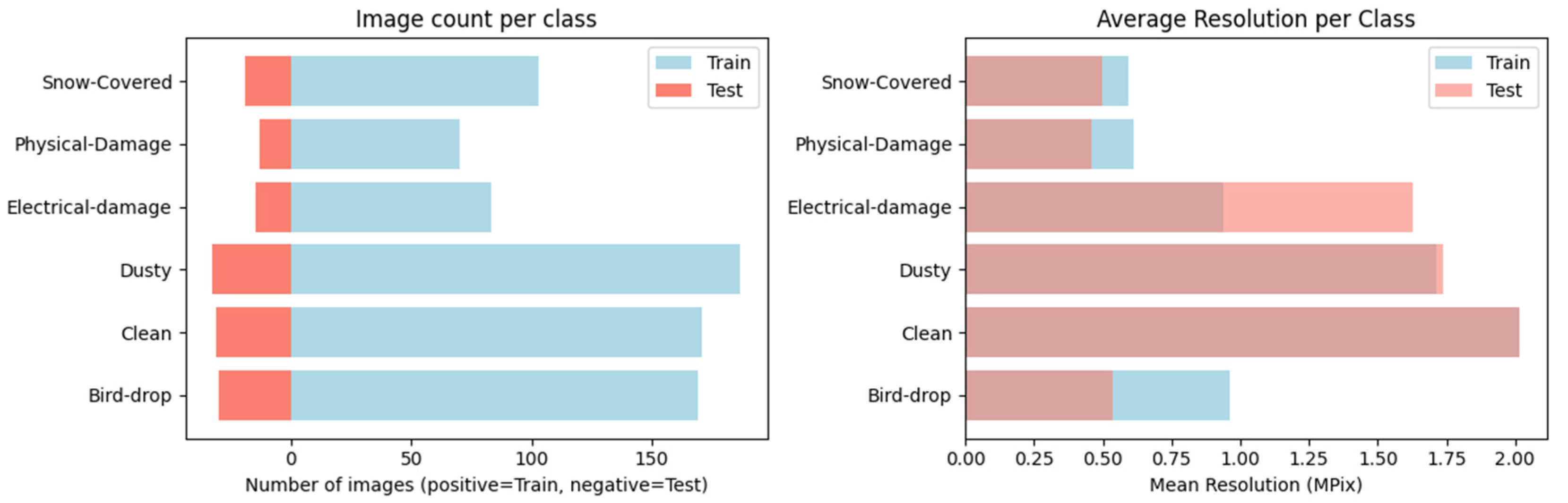
Figure 2.
Block-level representation of the convolutional neural network (CNN) architectures used in this study: Baseline CNN, EfficientNetB0, ResNet50, InceptionV3, and VGG16.
Figure 2.
Block-level representation of the convolutional neural network (CNN) architectures used in this study: Baseline CNN, EfficientNetB0, ResNet50, InceptionV3, and VGG16.
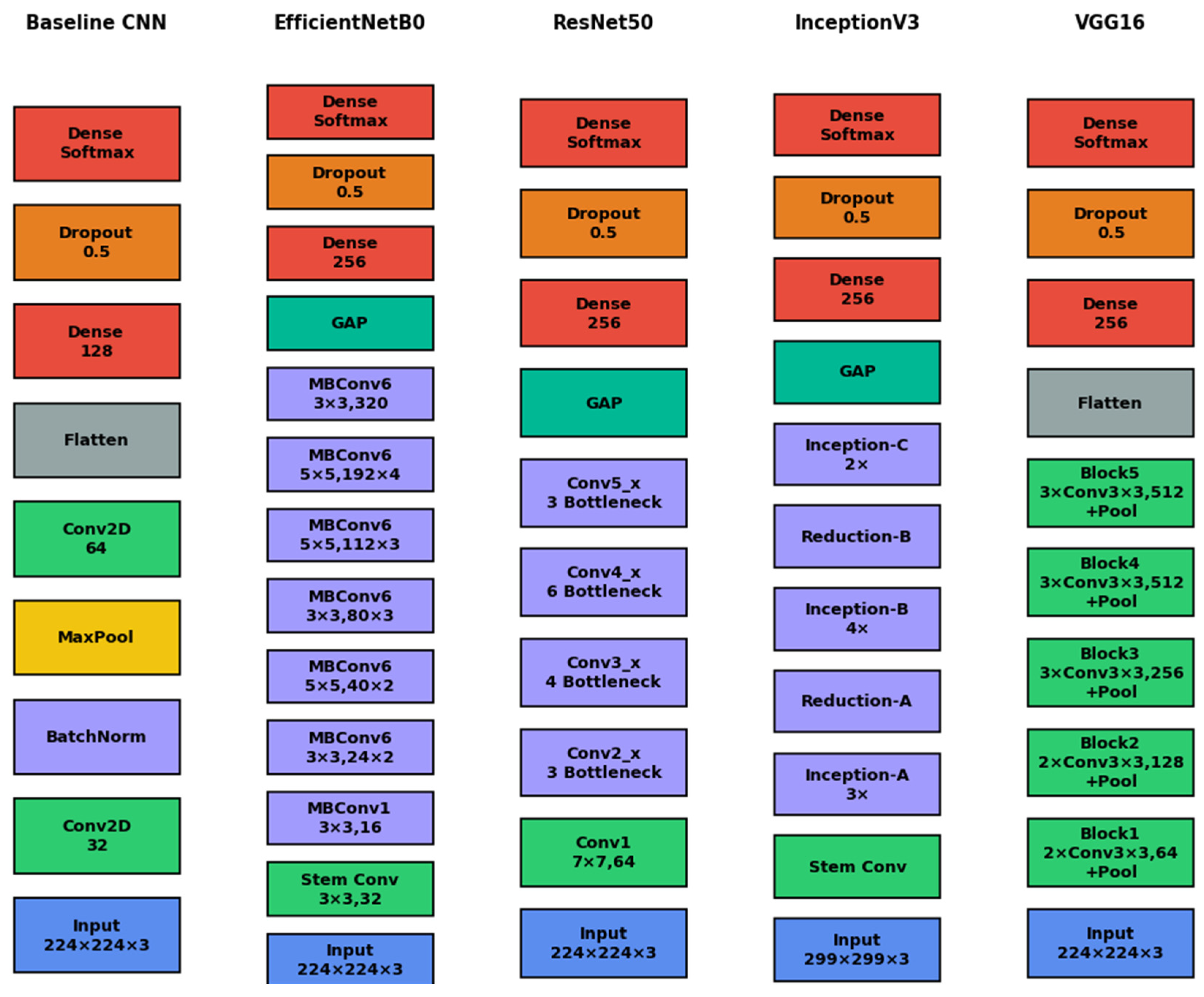
Figure 3.
Worst-tail LIME surrogate fidelity (mean ) across classes and architectures.
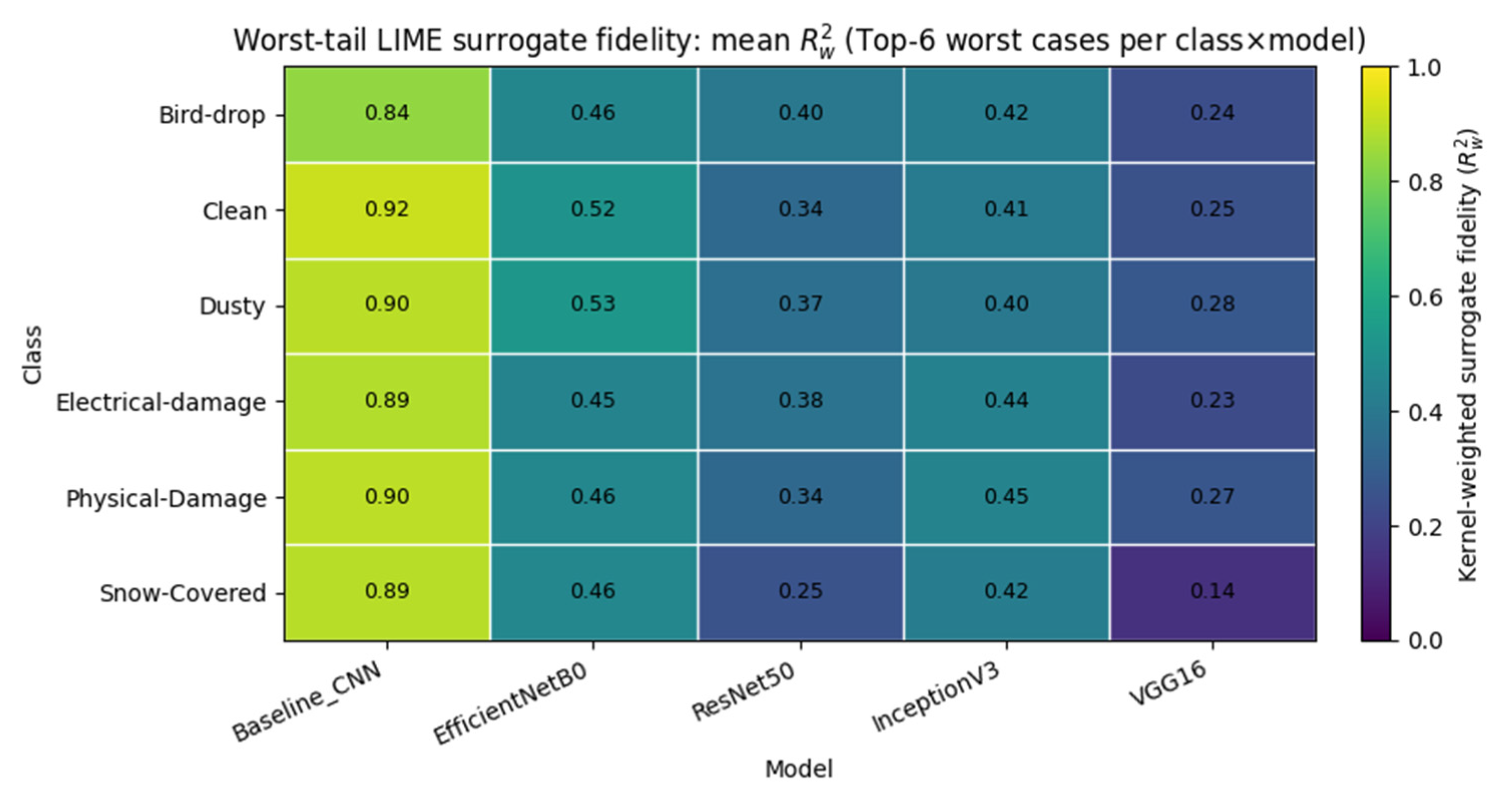
Figure 4.
Worst-tail LIME surrogate fidelity (minimum ) across classes and architectures.
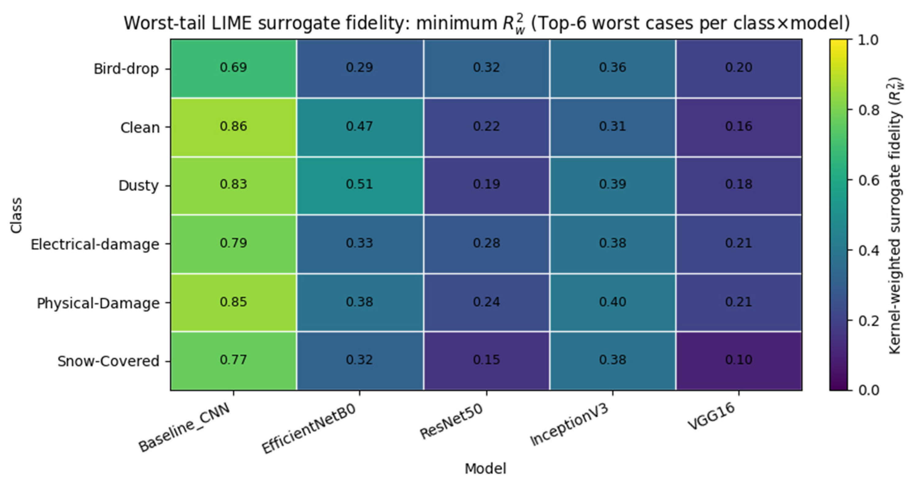
Figure 5.
Occlusion sensitivity for the Dust, Bird-drop, Electrical damage, Physical damage, and Snow-covered classes. Warmer colors indicate regions whose occlusion produces a larger decrease in the predicted-class score (higher functional relevance under masking).
Figure 5.
Occlusion sensitivity for the Dust, Bird-drop, Electrical damage, Physical damage, and Snow-covered classes. Warmer colors indicate regions whose occlusion produces a larger decrease in the predicted-class score (higher functional relevance under masking).
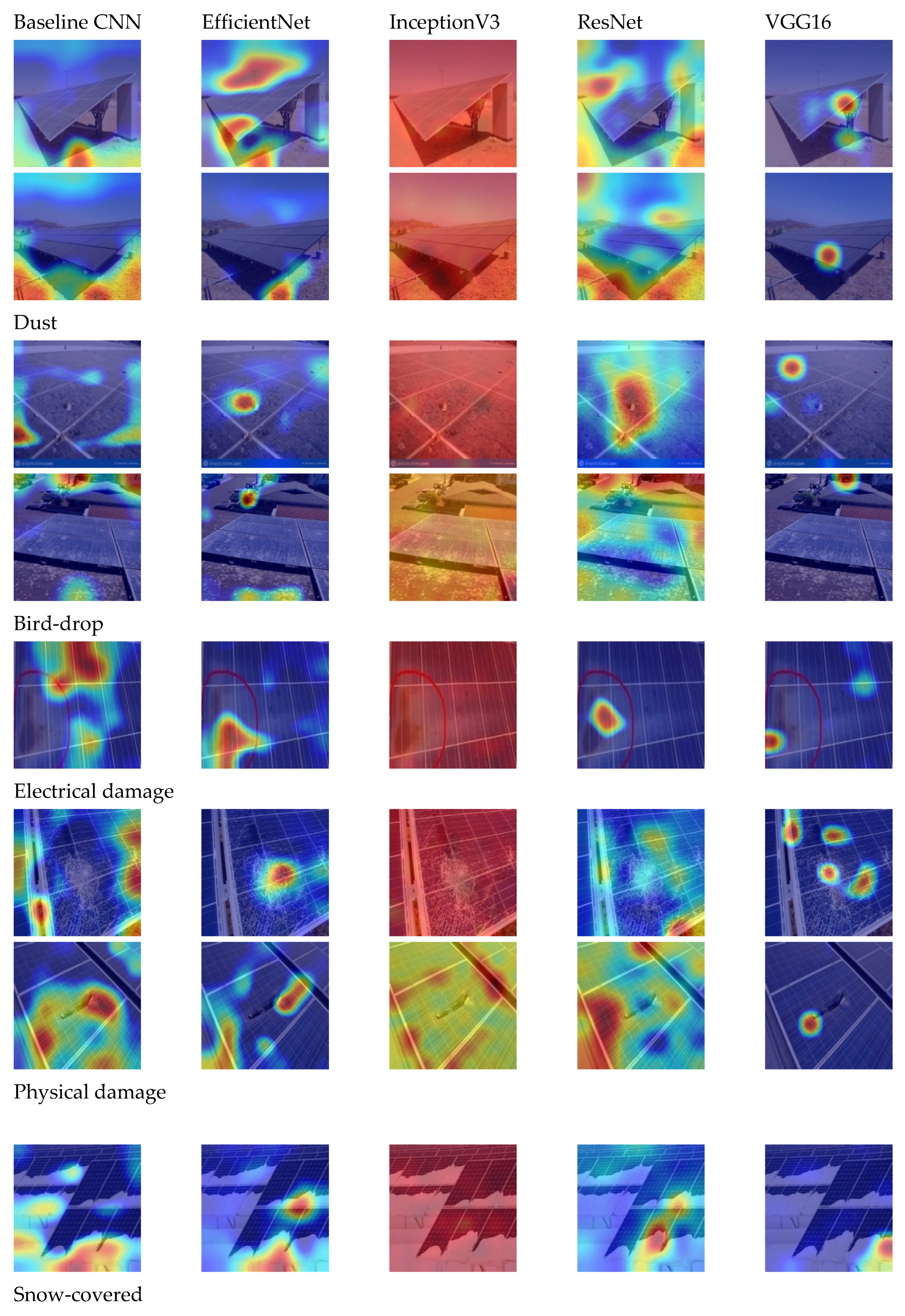
Figure 6.
Mean occlusion-map entropy for each architecture.

Figure 7.
Mean Hoyer sparsity across architectures.
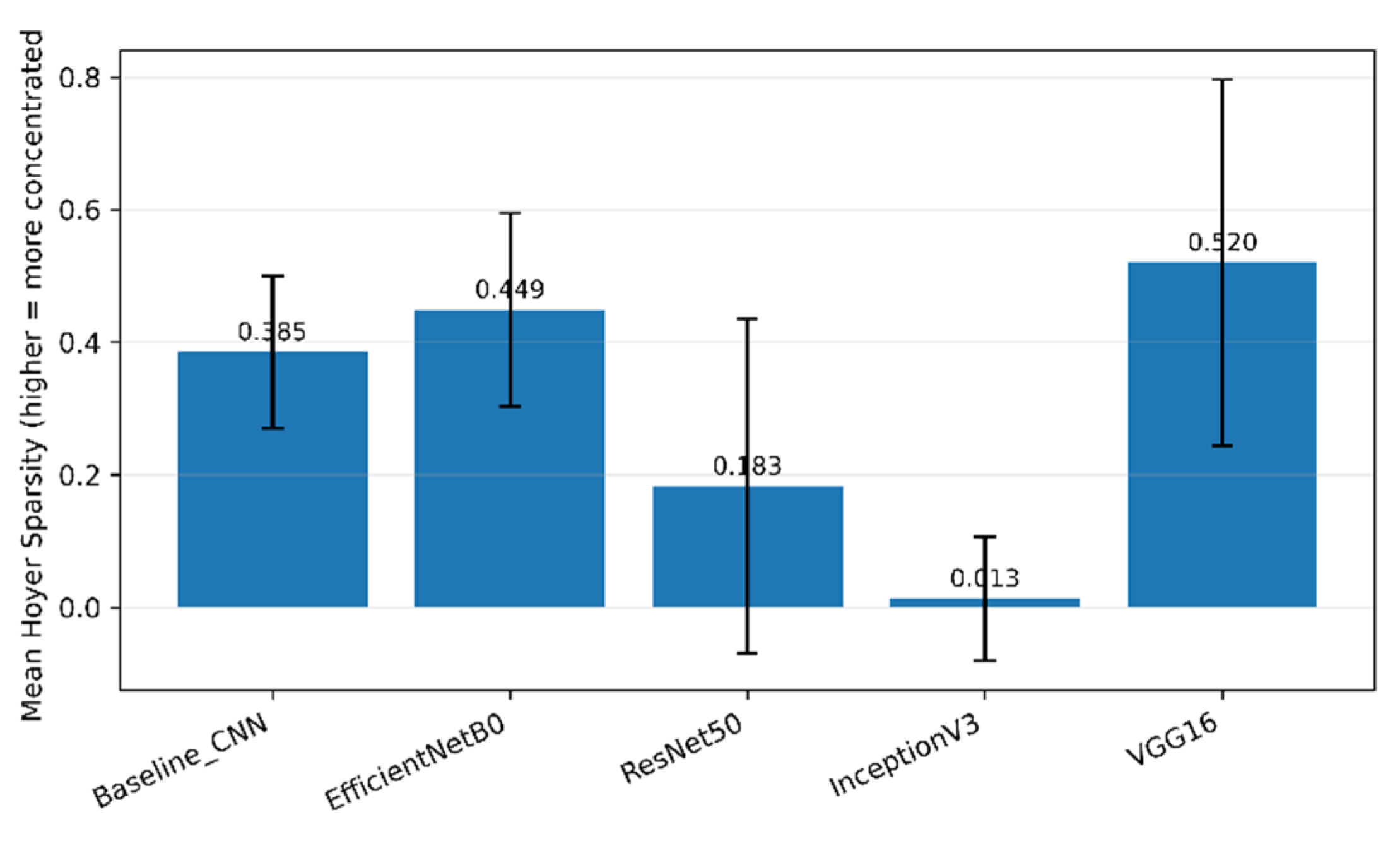
Figure 8.
Mean IoU@Top10% between model saliency and defect masks.
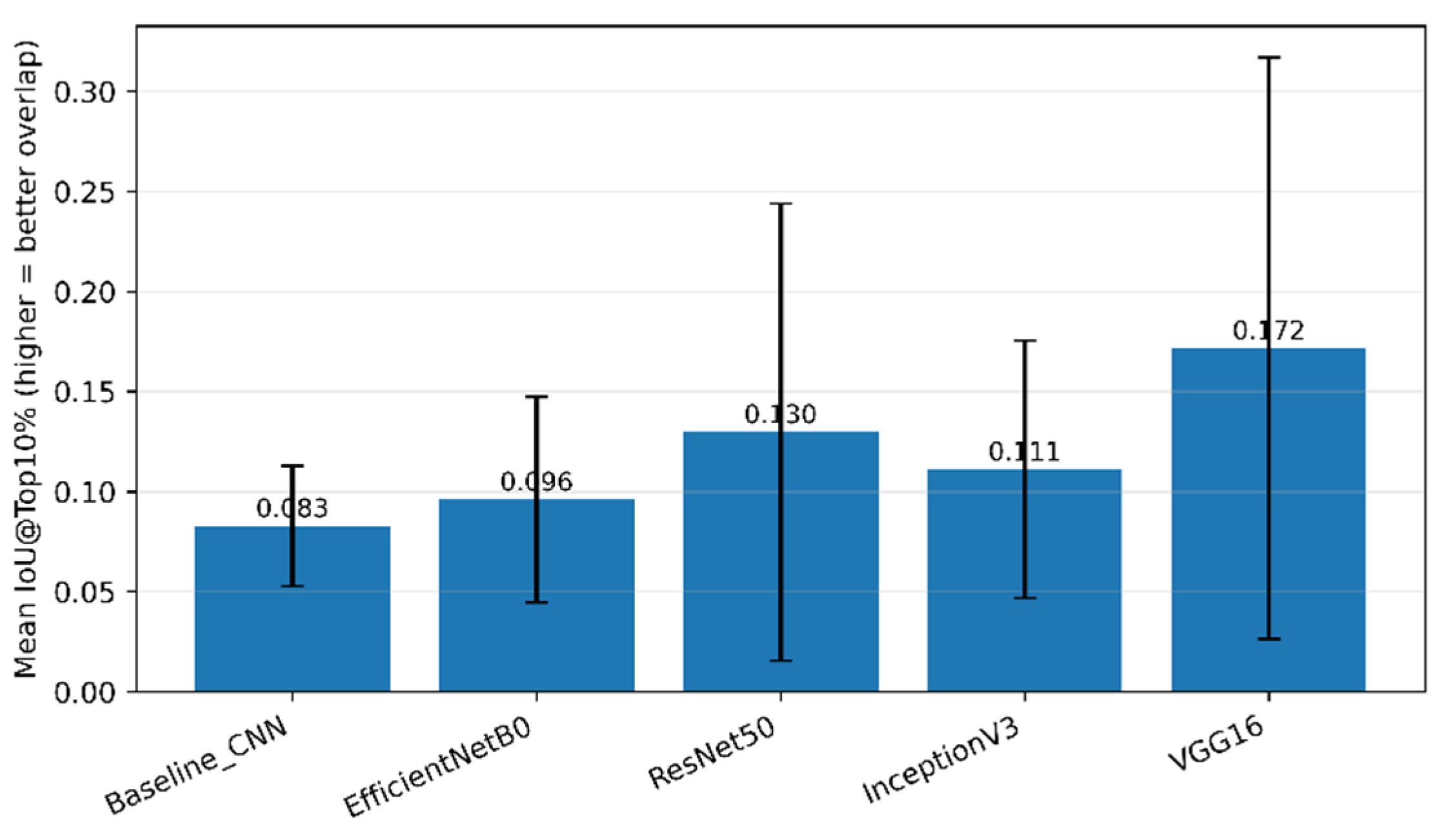
Figure 9.
Per-class IoU@Top10% for all architectures.
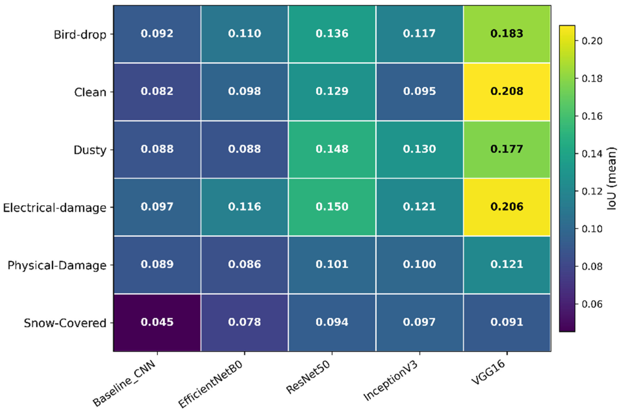
Figure 10.
Per-class Hoyer sparsity for all architectures.
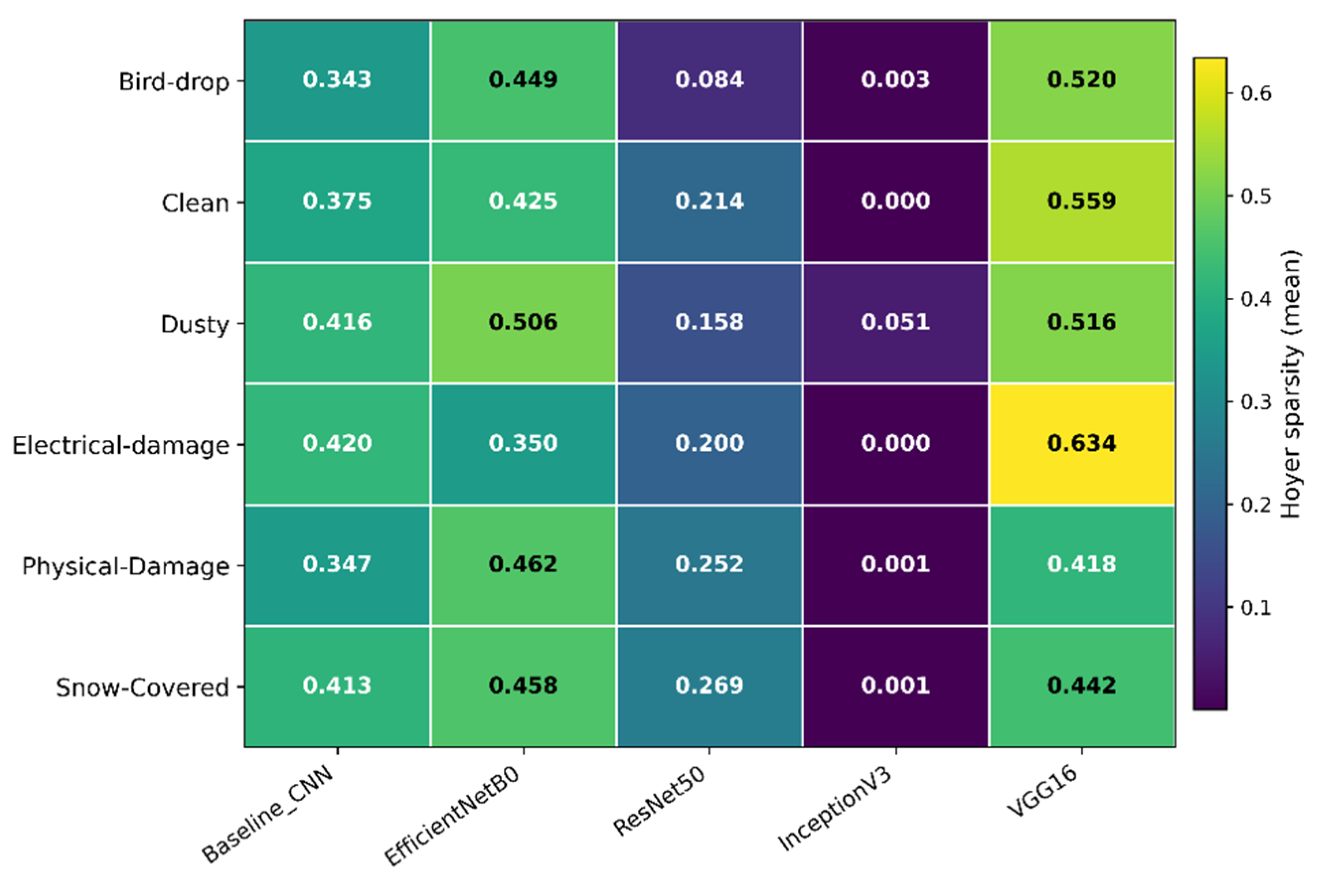
Figure 11.
Per-class entropy of occlusion sensitivity maps.
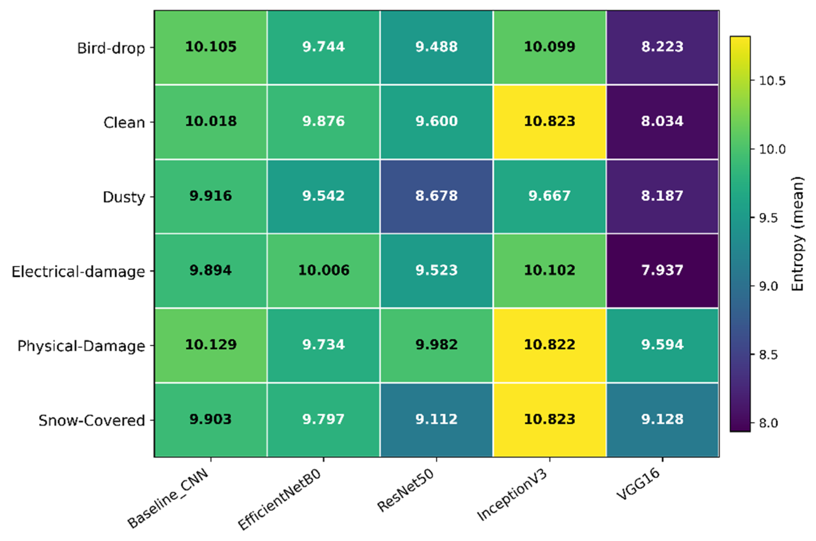
Figure 12.
Faithfulness gap averaged over all six classes for each architecture.
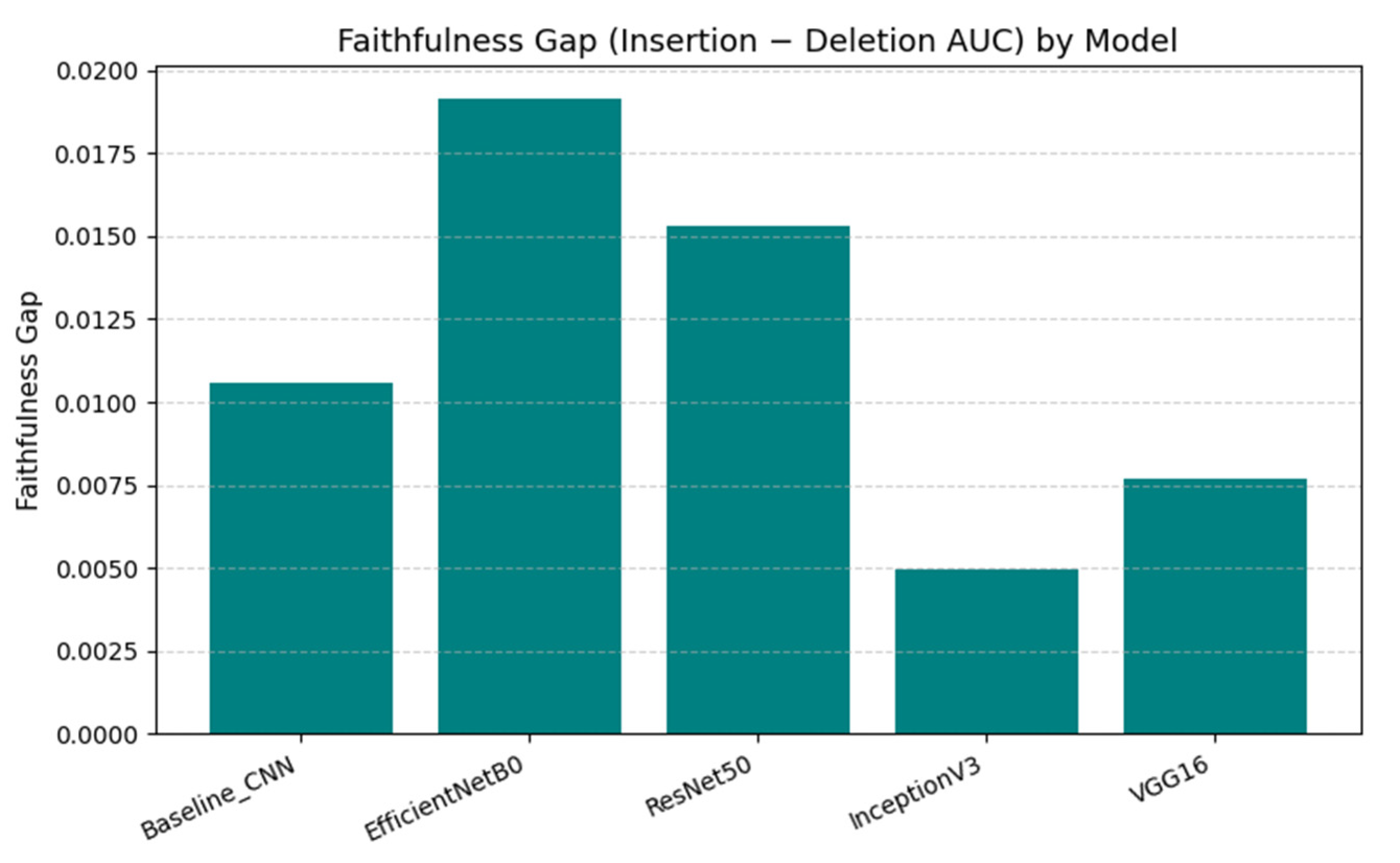
Figure 13.
Per-class Faithfulness Gap heatmap across all architectures.
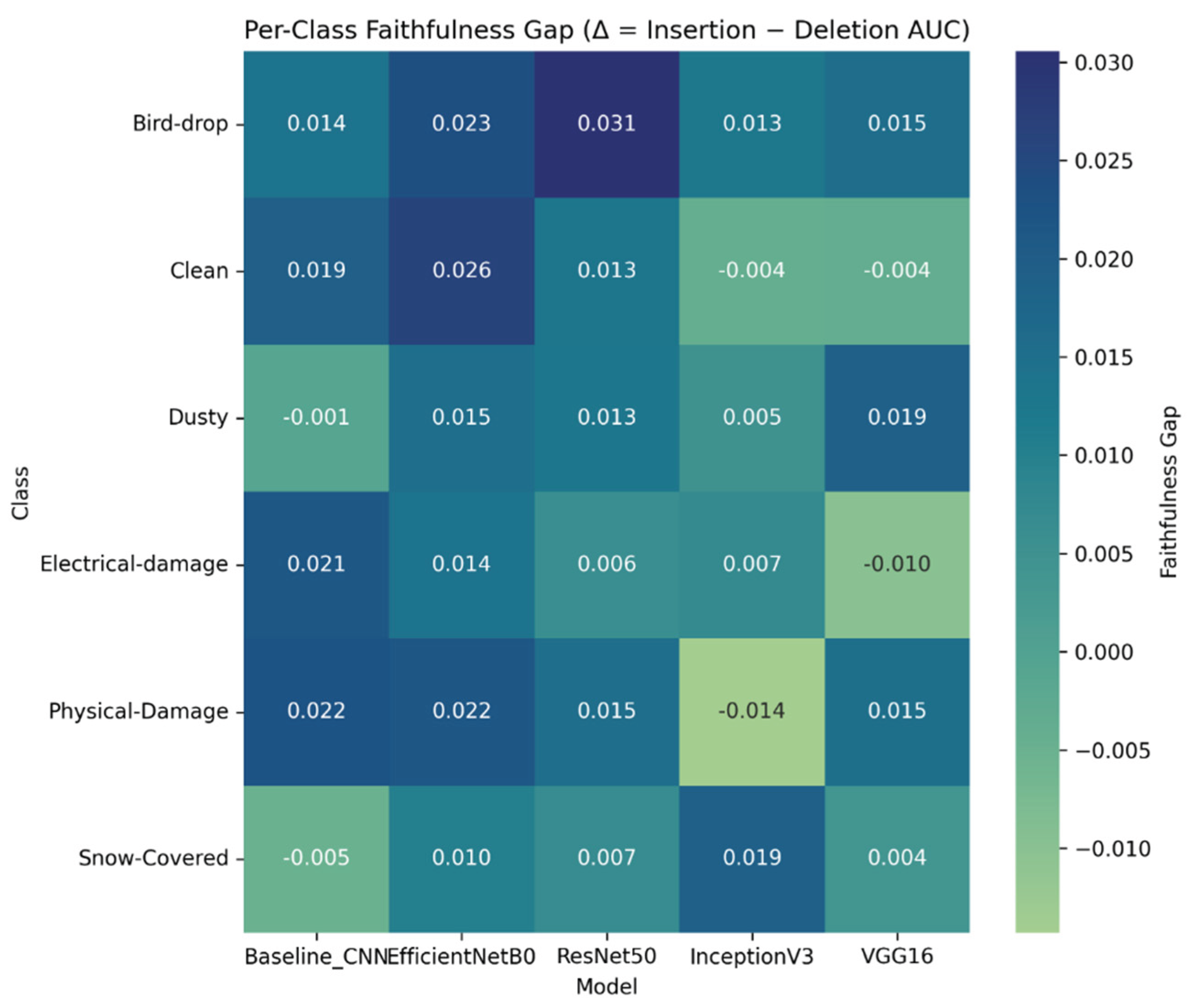
Table 3.
Quantitative occlusion-sensitivity interpretability metrics aggregated over the validation set ().
Table 3.
Quantitative occlusion-sensitivity interpretability metrics aggregated over the validation set ().
| Model | VGG16 | ResNet50 | InceptionV3 | EfficientNetB0 | Baseline_CNN |
| No images | 141 | 141 | 141 | 141 | 141 |
| IoU@Top10% | 0.172 ± 0.145 | 0.130 ± 0.114 | 0.111 ± 0.064 | 0.096 ± 0.051 | 0.083 ± 0.030 |
| Entropy | 8.391 ± 2.700 | 9.321 ± 3.157 | 10.321 ± 2.209 | 9.760 ± 0.555 | 9.994 ± 0.368 |
| HoyerSparsity | 0.520 ± 0.277 | 0.183 ± 0.252 | 0.013 ± 0.094 | 0.449 ± 0.146 | 0.385 ± 0.115 |
| PredProb | 0.887 ± 0.165 | 0.804 ± 0.186 | 0.674 ± 0.195 | 0.658 ± 0.197 | 0.550 ± 0.202 |
Table 4.
, , and faithfulness gap.
| Model | |||
| Baseline_CNN | 0.22594 | 0.23654 | 0.0106 |
| EfficientNetB0 | 0.22772 | 0.24688 | 0.0192 |
| ResNet50 | 0.25782 | 0.27314 | 0.0153 |
| InceptionV3 | 0.24359 | 0.24853 | 0.0049 |
| VGG16 | 0.26182 | 0.26949 | 0.0077 |
Disclaimer/Publisher’s Note: The statements, opinions and data contained in all publications are solely those of the individual author(s) and contributor(s) and not of MDPI and/or the editor(s). MDPI and/or the editor(s) disclaim responsibility for any injury to people or property resulting from any ideas, methods, instructions or products referred to in the content. |
© 2026 by the authors. Licensee MDPI, Basel, Switzerland. This article is an open access article distributed under the terms and conditions of the Creative Commons Attribution (CC BY) license (http://creativecommons.org/licenses/by/4.0/).
Copyright: This open access article is published under a Creative Commons CC BY 4.0 license, which permit the free download, distribution, and reuse, provided that the author and preprint are cited in any reuse.


