Application of Extended Dirac Equation to Photon–Electron Interactions and Electron–Positron Collision Processes: A Quantum Theoretical Approach Using a 256 × 256 Matrix Representation

1. Introduction

1.1. Background and Motivation

Photon–electron interactions and electron–electron/electron–positron collision processes constitute fundamental phenomena underlying atomic and particle physics. Compton scattering is indispensable for understanding interactions between X-rays or $\gamma$-rays and matter, and is widely used in analyzing radiation processes in astrophysical and laboratory plasmas [1,2]. Møller and Bhabha scattering serve as fundamental processes in electron beam experiments, playing important roles in accelerator physics and atomic collision experiments.

In relativistic quantum mechanics, these scattering processes are described by quantum electrodynamics (QED) based on the Dirac equation. In flat spacetime (Minkowski spacetime), an established theoretical framework exists [1,2]. However, how to extend the Dirac equation to curved spacetime in the presence of gravitational fields remains an important research topic [3,4].

The standard formulation of spinor fields in curved spacetime introduces vierbeins (tetrads) ${e^a}_{\mu }\left(x\right)$ and spin connections${{\omega }_{\mu }}^{ab}\left(x\right)$ [5,6]. While theoretically complete, practical scattering calculations often encounter the following difficulties:

• The choice of vierbein is not unique, potentially complicating calculations.
• The introduction of spin connections can obscure the correspondence with calculation rules in flat spacetime.
• Automation of numerical calculations becomes difficult.

1.2. Relevance to Atomic Physics and Collision Process Research

The method developed in this work can contribute to atomic physics and collision process research in the following aspects:

1.

Precision calculations of photon interactions: Cross-section calculations for Compton scattering are directly applicable to X-ray source and $\gamma$-ray detector design, dose calculations in medical physics, and related areas. This method enables systematic correction calculations including metric effects.

2.

Theoretical foundation for electron collision data: Precise theoretical calculations of Møller and Bhabha scattering are essential for luminosity measurements and detector calibration in electron beam experiments.

3.

Extension to exotic systems: Analysis of muon pair production connects to research on ${\mu }^{+}{\mu }^{-}$ atoms (muonium), exotic atoms, and applications in high-energy cosmic ray physics.

4.

Automation of calculations: In this method, geometric operations such as covariantization, connection-like operations, and basis transformations reduce to matrix products and trace calculations, facilitating automation of numerical calculations.

1.3. Our Approach: Metric Internalization into Matrices

To avoid these difficulties, we propose a new approach in this work. The basic idea is to embed the spacetime metric $g_{\mu \nu }\left(x\right)$ directly into gamma matrices. This enables construction of the Dirac equation in curved spacetime without explicitly introducing vierbeins.

Specifically, we extend the conventional $4\times 4$ gamma matrices ${\gamma }^{\mu }$ (4 matrices) and introduce 16 $256\times 256$ matrices ${{\mathrm{\Gamma }}_{\mu }}^{\nu }$. The key points are:

• The spacetime dimension remains 4; no extra dimensions are introduced.
• The number “16” corresponds to the number of basis elements of four-dimensional Dirac algebra ($2^4=16$).
• The metric tensor is incorporated as coefficients of the matrices.

1.4. Outline of the Formulation

This formulation proceeds through the following steps.

Step 1: Introduction of Two-Index Gamma Matrices

We construct constant (position-independent) basis matrices ${{\mathrm{\Gamma }}_{\mu }}^{\nu }$ ($\mu ,\nu =0,1,2,3$) as $256\times 256$ matrices.

Step 2: Metric Internalization

Using the spacetime metric $g_{\mu \nu }\left(x\right)$, we define position-dependent gamma matrices as

$${\mathrm{\Gamma }}_{\mu \nu }\left(x\right):={{\mathrm{\Gamma }}_{\mu }}^{\rho }{g}_{\rho \nu }\left(x\right).$$

(1)

This internalizes the metric information into the gamma matrix side.

Step 3: Construction of Effective Gamma Matrices

By summing the above 16 matrices along columns, we define the effective gamma matrices

$${\widehat{\mathrm{\Gamma }}}_{\nu }\left(x\right):=\sum _{\mu =0}^3{\mathrm{\Gamma }}_{\mu \nu }\left(x\right).$$

(2)

These 4 effective gamma matrices become the basic building blocks for the Dirac equation in curved spacetime.

Step 4: Dirac Operator

Using the effective gamma matrices, we extend the slash notation as

$$\cancel{p}\left(x\right):={\widehat{\mathrm{\Gamma }}}_{\nu }\left(x\right)p^{\nu }$$

(3)

and define the Dirac operator as

$$D\left(x\right):={\widehat{\mathrm{\Gamma }}}_{\nu }\left(x\right){\partial }^{\nu }.$$

(4)

The slash notation (Equation (3)) and Dirac operator (Equation (4)) form the foundation of this extended formalism.

1.5. Consistency with Flat Spacetime

An important property of this approach is that it exactly reproduces standard results in the flat spacetime limit. When the metric approaches the Minkowski metric, $g_{\mu \nu }\left(x\right)\to {\eta }_{\mu \nu }$, we have

$${\mathrm{\Gamma }}_{\mu \nu }\left(x\right)\to {{\mathrm{\Gamma }}_{\mu }}^{\rho }{\eta }_{\rho \nu },{\widehat{\mathrm{\Gamma }}}_{\nu }\left(x\right)\to \sum _{\mu }{{\mathrm{\Gamma }}_{\mu }}^{\rho }{\eta }_{\rho \nu },$$

and under appropriate normalization, the $256\times 256$ representation matches the standard $4\times 4$ representation.

We numerically verified this consistency for all scattering processes treated in this paper:

• Compton scattering (photon–electron scattering) (Section 5);
• Muon pair production (Appendix B);
• Møller scattering (electron–electron collision) (Appendix C);
• Bhabha scattering (electron–positron collision) (Appendix D).

In each case, we confirmed agreement with standard QED results [1,2,8] including the Klein–Nishina formula [7].

1.6. Main Contributions of This Work

The main contributions of this paper are as follows:

1.

New formulation: Construction of two-index gamma matrices directly embedding the metric, and introduction of matrix-valued Dirac operator based on effective gamma ${\widehat{\mathrm{\Gamma }}}^{\mu }\left(x\right)$ (Equation (2)).

2.

Systematization of calculations: Feynman rules derived from the extended QED Lagrangian (Equation (5)) and procedures suitable for automation.

3.

Numerical verification: Trial calculations using a metric with off-diagonal components (toy model) showing that characteristic corrections can appear in the angular dependence of differential cross sections, while confirming exact agreement in the flat limit [9,10,11].

1.7. Comparison of Conventional and Extended Dirac Equations

To visualize the structure of the proposed method, we compare the conventional Dirac equation with the extended version in matrix form.

Conventional Dirac Equation (Flat Spacetime)

In flat spacetime, using 4 $4\times 4$ gamma matrices ${\gamma }^{\mu }$,

$$\left(i{\gamma }^{\mu }{\partial }_{\mu }-m\right)\psi \left(x\right)=0.$$

The gamma matrices satisfy

$$\{{\gamma }^{\mu },{\gamma }^{\nu }\}=2{\eta }^{\mu \nu }{I}_4,{\eta }_{\mu \nu }=\mathrm{diag}(+1,-1,-1,-1).$$

In flat spacetime, since ${\eta }_{\mu \nu }$ is diagonal, a diagonal arrangement of gamma matrices suffices.

Extended Dirac Equation (Curved Spacetime)

In curved spacetime, the metric $g_{\mu \nu }\left(x\right)$ generally has off-diagonal components. To accommodate this, we use 16 $256\times 256$ matrices ${{\mathrm{\Gamma }}_{\mu }}^{\nu }$ and multiply directly by the metric:

$$\begin{array}{cc}\hfill & i{{\mathrm{\Gamma }}_{\mu }}^{\rho }{g}_{\rho \nu }\left(x\right){\partial }^{\nu }-m{I}_{256}=i{\mathrm{\Gamma }}_{\mu \nu }\left(x\right){\partial }^{\nu }-m{I}_{256}\hfill \end{array}$$

(5)

where ${\mathrm{\Gamma }}_{\mu \nu }\left(x\right):={{\mathrm{\Gamma }}_{\mu }}^{\rho }{g}_{\rho \nu }\left(x\right)$.

The advantages of this construction are:

• Off-diagonal components of the metric are naturally incorporated.
• No need to explicitly introduce vierbeins.
• Calculation rules are unified through matrix products and traces.
• Standard results are automatically recovered in the flat limit.

1.8. Paper Organization

The remainder of this paper is organized as follows. Section 2 provides the explicit construction of the $256\times 256$ matrix representation. Section 3 discusses consistency under general coordinate transformations. Section 4 introduces the extended QED Lagrangian and corresponding Feynman rules. Section 5 calculates Compton scattering as a representative example and compares with flat spacetime results. Section 6 discusses the focus, scope of applicability, advantages, and limitations of this method, and Section 7 presents conclusions. Additional processes (muon pair production, Møller scattering, Bhabha scattering) and Mathematica code are summarized in the appendices.

2. Construction of the $256\times 256$ Matrix Representation

2.1. Why a $256\times 256$ Representation with 16 Basis Matrices Is Needed

This section explains the construction of the $256\times 256$ matrix representation and clarifies why it is needed and what mathematical background underlies it.

2.1.0.7. Number of Dirac Algebra Basis Elements

In four-dimensional spacetime, the Dirac (gamma matrix) algebra has $2^4=16$ independent basis elements. In the conventional $4\times 4$ representation, these are expressed as products of 4 ${\gamma }^{\mu }$ matrices.

Motivation for Two-Index Representation

In this work, we multiply the metric $g_{\mu \nu }\left(x\right)$ directly into the gamma matrices. For this purpose, we label gamma matrices with two indices$(\mu ,\nu )$. Since $\mu ,\nu =0,1,2,3$, there are $4\times 4=16$ combinations, corresponding to the “16 basis matrices” used in this work.

Why $256\times 256$

To explicitly realize each basis matrix ${{\mathrm{\Gamma }}_{\mu }}^{\nu }$, we use Kronecker (tensor) products of Pauli matrices. An 8-fold tensor product of $2\times 2$ matrices gives

$$2^8=256,$$

hence we obtain a $256\times 256$ matrix representation. This construction yields 16 mutually independent basis matrices satisfying the required anticommutation relations.

2.2. Kronecker Product Construction Using Pauli Matrices

Using the $2\times 2$ identity matrix e and Pauli matrices

$${\sigma }_x=\left(\begin{array}{cc}0& 1\\ 1& 0\end{array}\right),{\sigma }_y=\left(\begin{array}{cc}0& -i\\ i& 0\end{array}\right),{\sigma }_z=\left(\begin{array}{cc}1& 0\\ 0& -1\end{array}\right)$$

as building blocks, we construct the basis matrices via 8-fold Kronecker products (⊗):

$$\begin{array}{cc}\hfill {{\mathrm{\Gamma }}_0}^0& ={\sigma }_x\otimes {\sigma }_x\otimes {\sigma }_x\otimes {\sigma }_x\otimes {\sigma }_x\otimes {\sigma }_x\otimes {\sigma }_x\otimes {\sigma }_x\hfill \\ \hfill {{\mathrm{\Gamma }}_0}^1& =i{\sigma }_x\otimes {\sigma }_x\otimes {\sigma }_x\otimes {\sigma }_x\otimes {\sigma }_x\otimes {\sigma }_x\otimes {\sigma }_x\otimes {\sigma }_y\hfill \\ \hfill {{\mathrm{\Gamma }}_0}^2& =i{\sigma }_x\otimes {\sigma }_x\otimes {\sigma }_x\otimes {\sigma }_x\otimes {\sigma }_x\otimes {\sigma }_x\otimes {\sigma }_x\otimes {\sigma }_z\hfill \\ \hfill {{\mathrm{\Gamma }}_0}^3& =i{\sigma }_y\otimes {\sigma }_z\otimes {\sigma }_z\otimes {\sigma }_z\otimes {\sigma }_z\otimes {\sigma }_z\otimes {\sigma }_z\otimes {\sigma }_z\hfill \\ \hfill {{\mathrm{\Gamma }}_1}^0& =i{\sigma }_x\otimes {\sigma }_x\otimes {\sigma }_y\otimes {\sigma }_z\otimes {\sigma }_z\otimes {\sigma }_z\otimes {\sigma }_z\otimes {\sigma }_z\hfill \\ \hfill {{\mathrm{\Gamma }}_1}^1& =i{\sigma }_x\otimes {\sigma }_x\otimes {\sigma }_x\otimes {\sigma }_x\otimes {\sigma }_z\otimes {\sigma }_z\otimes {\sigma }_z\otimes {\sigma }_z\hfill \\ \hfill {{\mathrm{\Gamma }}_1}^2& =i{\sigma }_x\otimes {\sigma }_x\otimes {\sigma }_x\otimes {\sigma }_x\otimes {\sigma }_x\otimes {\sigma }_z\otimes {\sigma }_z\otimes {\sigma }_z\hfill \\ \hfill {{\mathrm{\Gamma }}_1}^3& =i{\sigma }_x\otimes {\sigma }_x\otimes {\sigma }_x\otimes {\sigma }_x\otimes {\sigma }_x\otimes {\sigma }_x\otimes {\sigma }_y\otimes {\sigma }_z\hfill \\ \hfill {{\mathrm{\Gamma }}_2}^0& =i{\sigma }_z\otimes {\sigma }_z\otimes {\sigma }_z\otimes {\sigma }_z\otimes {\sigma }_z\otimes {\sigma }_z\otimes {\sigma }_z\otimes {\sigma }_z\hfill \\ \hfill {{\mathrm{\Gamma }}_2}^1& =i{\sigma }_x\otimes {\sigma }_x\otimes {\sigma }_x\otimes {\sigma }_x\otimes {\sigma }_y\otimes {\sigma }_z\otimes {\sigma }_z\otimes {\sigma }_z\hfill \\ \hfill {{\mathrm{\Gamma }}_2}^2& =i{\sigma }_x\otimes {\sigma }_x\otimes {\sigma }_x\otimes {\sigma }_y\otimes {\sigma }_z\otimes {\sigma }_z\otimes {\sigma }_z\otimes {\sigma }_z\hfill \\ \hfill {{\mathrm{\Gamma }}_2}^3& =i{\sigma }_x\otimes {\sigma }_x\otimes {\sigma }_x\otimes {\sigma }_x\otimes {\sigma }_x\otimes {\sigma }_y\otimes {\sigma }_z\otimes {\sigma }_z\hfill \\ \hfill {{\mathrm{\Gamma }}_3}^0& =i{\sigma }_x\otimes {\sigma }_y\otimes {\sigma }_z\otimes {\sigma }_z\otimes {\sigma }_z\otimes {\sigma }_z\otimes {\sigma }_z\otimes {\sigma }_z\hfill \\ \hfill {{\mathrm{\Gamma }}_3}^1& =i{\sigma }_x\otimes {\sigma }_z\otimes {\sigma }_z\otimes {\sigma }_z\otimes {\sigma }_z\otimes {\sigma }_z\otimes {\sigma }_z\otimes {\sigma }_z\hfill \\ \hfill {{\mathrm{\Gamma }}_3}^2& =i{\sigma }_x\otimes {\sigma }_x\otimes {\sigma }_x\otimes {\sigma }_z\otimes {\sigma }_z\otimes {\sigma }_z\otimes {\sigma }_z\otimes {\sigma }_z\hfill \\ \hfill {{\mathrm{\Gamma }}_3}^3& =i{\sigma }_x\otimes {\sigma }_x\otimes {\sigma }_z\otimes {\sigma }_z\otimes {\sigma }_z\otimes {\sigma }_z\otimes {\sigma }_z\otimes {\sigma }_z\hfill \end{array}$$

(6)

This construction follows standard references on Clifford algebras and spinors [12,13,14,15].

2.3. Anticommutation Relations

The 16 basis matrices satisfy the following anticommutation relation:

$$\begin{array}{c}\hfill \{{{\mathrm{\Gamma }}_{\mu }}^{\nu },{{\mathrm{\Gamma }}_{\rho }}^{\sigma }\}=2{{\delta }^{\nu }}_{\sigma }{\eta }_{\mu \rho }{I}_{256}.\end{array}$$

(7)

This can be interpreted as follows:

• When right indices match ($\nu =\sigma$): For each fixed column index, $\{{{\mathrm{\Gamma }}_{\mu }}^{\nu },{{\mathrm{\Gamma }}_{\rho }}^{\nu }\}=2{\eta }_{\mu \rho }{I}_{256}$ holds. Thus, $\mu =\rho =0$ gives $+2I_{256}$, $\mu =\rho =i$ ($i=1,2,3$) gives $-2I_{256}$, and $\mu \ne \rho$ gives 0.
• When right indices differ ($\nu \ne \sigma$): $\{{{\mathrm{\Gamma }}_{\mu }}^{\nu },{{\mathrm{\Gamma }}_{\rho }}^{\sigma }\}=0$.

Lowering indices via ${\mathrm{\Gamma }}_{\mu \nu }:={{\mathrm{\Gamma }}_{\mu }}^{\alpha }{\eta }_{\alpha \nu }$, Equation (7) equivalently becomes

$$\begin{array}{c}\hfill \{{\mathrm{\Gamma }}_{\mu \nu },{\mathrm{\Gamma }}_{\rho \sigma }\}=2{\eta }_{\mu \rho }{\eta }_{\nu \sigma }{I}_{256}.\end{array}$$

(8)

This covariant form is useful for checking index consistency.

2.4. Metric Internalization and Effective Gamma Matrices

The spacetime metric $g_{\mu \nu }\left(x\right)$ is internalized into the matrix side through the mixed-index basis ${{\mathrm{\Gamma }}_{\mu }}^{\nu }$:

$${\mathrm{\Gamma }}_{\mu \nu }\left(x\right){{\mathrm{\Gamma }}_{\mu }}^{\rho }{g}_{\rho \nu }\left(x\right).$$

Upper-index forms are defined as

$${{\mathrm{\Gamma }}^{\mu }}_{\nu }\left(x\right)g^{\mu \rho }\left(x\right){\mathrm{\Gamma }}_{\rho \nu }\left(x\right),{\mathrm{\Gamma }}^{\mu \nu }\left(x\right)g^{\mu \rho }\left(x\right)g^{\nu \sigma }\left(x\right){\mathrm{\Gamma }}_{\rho \sigma }\left(x\right).$$

By Equation (2), the effective gamma matrices are defined as

$${\widehat{\mathrm{\Gamma }}}_{\nu }\left(x\right)\sum _{\mu =0}^3{\mathrm{\Gamma }}_{\mu \nu }\left(x\right).$$

This operation combines the 16 basis matrices along columns, yielding 4 matrices that serve as the fundamental objects for the Dirac equation in curved spacetime.

The slash notation is

$$\cancel{p}\left(x\right){\widehat{\mathrm{\Gamma }}}_{\nu }\left(x\right)p^{\nu },$$

and thus the matrix-valued Dirac operator

$$D\left(x\right){\widehat{\mathrm{\Gamma }}}_{\nu }\left(x\right){\partial }^{\nu }$$

is naturally obtained. Calculations can be performed through matrix products and traces (see also [16,17] for related motivations in geometric algebra).

2.5. Anticommutation Relation for Effective Gamma

From ${\mathrm{\Gamma }}_{\mu \nu }\left(x\right)={{\mathrm{\Gamma }}_{\mu }}^{\rho }{g}_{\rho \nu }\left(x\right)$ and ${\widehat{\mathrm{\Gamma }}}_{\nu }\left(x\right)={\sum }_{\mu }{\mathrm{\Gamma }}_{\mu \nu }\left(x\right)$, the effective gamma satisfies

$$\{{\widehat{\mathrm{\Gamma }}}_{\mu }\left(x\right),{\widehat{\mathrm{\Gamma }}}_{\nu }\left(x\right)\}=2g_{\mu \nu }\left(x\right)I_{256}.$$

(9)

Importantly, metric weighting occurs only once (at the stage ${\mathrm{\Gamma }}_{\mu \nu }\left(x\right)={{\mathrm{\Gamma }}_{\mu }}^{\rho }{g}_{\rho \nu }\left(x\right)$). No additional weighting is applied during the column sum for ${\widehat{\mathrm{\Gamma }}}_{\nu }\left(x\right)$. This ensures the right-hand side is linear in $g_{\mu \nu }\left(x\right)$, avoiding double counting equivalent to $g^2$.

In the flat limit $g_{\mu \nu }\to {\eta }_{\mu \nu }$, we recover $\{{\widehat{\mathrm{\Gamma }}}_{\mu },{\widehat{\mathrm{\Gamma }}}_{\nu }\}\to 2{\eta }_{\mu \nu }{I}_{256}$, corresponding to the standard 4 gamma matrices.

2.6. Numerical Verification

Using the Mathematica program shown in Appendix E, we numerically verified Equations (7) and (9) through determinant checks (orthogonality and scale $2^{256}$) and trace checks (including signs of ${\eta }_{\mu \rho }$). Under appropriate phase normalization, $\{{{\mathrm{\Gamma }}_{\mu }}^{\nu },{{\mathrm{\Gamma }}_{\rho }}^{\sigma }\}=2{{\delta }^{\nu }}_{\sigma }{\eta }_{\mu \rho }{I}_{256}$ is numerically confirmed.

2.7. Slash Identity and Propagator Kernel

Let $\cancel{p}\left(x\right)={\widehat{\mathrm{\Gamma }}}_{\nu }\left(x\right)p^{\nu }$. Then the slash identity holds:

$$\cancel{p}\left(x\right)\cancel{p}\left(x\right)=\frac{1}{2}\{{\widehat{\mathrm{\Gamma }}}_{\mu }\left(x\right),{\widehat{\mathrm{\Gamma }}}_{\nu }\left(x\right)\}{p}^{\mu }{p}^{\nu }=g_{\mu \nu }\left(x\right)p^{\mu }{p}^{\nu }{I}_{256}\equiv p^2\left(x\right)I_{256},$$

(10)

yielding $(\cancel{p}-m)(\cancel{p}+m)=p^2-m^2$. Thus the fermion propagator is

$$S_F(p;x)=i{(\cancel{p}\left(x\right)-m+iϵ)}^{-1},p^2\left(x\right)=g_{\mu \nu }\left(x\right)p^{\mu }{p}^{\nu }.$$

2.8. Note on Normalization

When comparing with the standard $4\times 4$ formalism, one must track normalization factors arising from the difference between ${\mathrm{tr}}_{256}\left(I_{256}\right)=256$ and ${\mathrm{tr}}_4\left(I_4\right)=4$. In the flat limit, fixing trace normalization yields a unique correspondence between $256\times 256$ results and standard $4\times 4$ formulas.

3. Consistency Under General Coordinate Transformations

The metric tensor appearing in Equation (5)

$$g_{\mu \nu }\left(x\right)=\left[\begin{array}{cccc}{g}_{00}\left(x\right)& g_{01}\left(x\right)& g_{02}\left(x\right)& g_{03}\left(x\right)\\ g_{10}\left(x\right)& g_{11}\left(x\right)& g_{12}\left(x\right)& g_{13}\left(x\right)\\ g_{20}\left(x\right)& g_{21}\left(x\right)& g_{22}\left(x\right)& g_{23}\left(x\right)\\ g_{30}\left(x\right)& g_{31}\left(x\right)& g_{32}\left(x\right)& g_{33}\left(x\right)\end{array}\right]$$

transforms under general coordinate transformations

$$x^{\mu }\to x^{\prime \mu }=x^{\prime \mu }\left(x\right)$$

as a rank-2 covariant tensor:

$$g_{\alpha \beta }^{\prime }\left(x^{\prime }\right)={\displaystyle \frac{\partial x^{\mu }}{\partial x^{\prime \alpha }}}{\displaystyle \frac{\partial x^{\nu }}{\partial x^{\prime \beta }}}{g}_{\mu \nu }\left(x\right).$$

The inverse metric transforms as

$$g^{\prime \alpha \beta }\left(x^{\prime }\right)={\displaystyle \frac{\partial x^{\prime \alpha }}{\partial x^{\mu }}}{\displaystyle \frac{\partial x^{\prime \beta }}{\partial x^{\nu }}}{g}^{\mu \nu }\left(x\right),g_{\mu \nu }{g}^{\nu \rho }={\delta }_{\mu }^{\rho }.$$

Under these transformation rules, physical scalars (inner products, actions, $d{s}^2=g_{\mu \nu }d{x}^{\mu }d{x}^{\nu }$) are invariant, and the $4\times 4$ matrix representation constructed from metric components behaves covariantly according to tensor transformation rules.

The effective gamma matrices transform as covariant vectors:

$${\widehat{\mathrm{\Gamma }}}_{\alpha }^{\prime }\left(x^{\prime }\right)={\displaystyle \frac{\partial x^{\nu }}{\partial x^{\prime \alpha }}}{\widehat{\mathrm{\Gamma }}}_{\nu }\left(x\right).$$

(11)

Here the basis matrices ${{\mathrm{\Gamma }}_{\mu }}^{\nu }$ themselves are fixed, and their coefficients change. Equation (9) preserves its form under this transformation, and $\cancel{p}={\widehat{\mathrm{\Gamma }}}_{\nu }{p}^{\nu }$ remains a scalar.

4. Extended QED Lagrangian and Feynman Rules

In this section, we use the matrix-valued Dirac operator defined in the previous section

$$D\left(x\right)={\widehat{\mathrm{\Gamma }}}_{\nu }\left(x\right){\partial }^{\nu },{\widehat{\mathrm{\Gamma }}}_{\nu }\left(x\right)=\sum _{\mu =0}^3{\mathrm{\Gamma }}_{\mu \nu }\left(x\right),{\mathrm{\Gamma }}_{\mu \nu }\left(x\right)={{\mathrm{\Gamma }}_{\mu }}^{\rho }{g}_{\rho \nu }\left(x\right)$$

and adopt QED-type minimal coupling to the electromagnetic field. Gravitational (metric) effects are internalized into the matrix side through ${\mathrm{\Gamma }}_{\mu \nu }\left(x\right)$ and ${\widehat{\mathrm{\Gamma }}}_{\nu }\left(x\right)$.

4.1. Extended QED Lagrangian

The Lagrangian density is

$$\mathcal{L}=\overline{\Psi }\left(i{\widehat{\mathrm{\Gamma }}}_{\nu }\left(x\right)\left[{\partial }^{\nu }+ie{A}^{\nu }\left(x\right)\right]-m\right)\Psi -{\displaystyle \frac{1}{4}}{F}_{\mu \nu }{F}^{\mu \nu },$$

(12)

where $F_{\mu \nu }={\partial }_{\mu }{A}_{\nu }-{\partial }_{\nu }{A}_{\mu }$, and index raising/lowering is done with $g_{\mu \nu }\left(x\right)$ and its inverse $g^{\mu \nu }\left(x\right)$. In the flat limit $g_{\mu \nu }\left(x\right)\to {\eta }_{\mu \nu }$, ${\widehat{\mathrm{\Gamma }}}_{\nu }\left(x\right)$ reduces to the flat reference ${\widehat{\gamma }}_{\nu }$, and standard QED is recovered.

4.2. Feynman Rules

The Feynman rules are derived from the extended QED Lagrangian (Equation (12)). The rules used in this paper’s calculations (processing external line spin sums via traces) are:

• Vertex: $-ie{\widehat{\mathrm{\Gamma }}}_{\nu }\left(x\right)$. Here $\nu$ is the Lorentz index of the external photon. The effective gamma ${\widehat{\mathrm{\Gamma }}}_{\nu }\left(x\right)$ is used directly as the vertex operator.
• Fermion propagator: $S_F\left(p\right)=i{(\cancel{p}-m+iϵ)}^{-1}$, where $\cancel{p}\left(x\right)\equiv {\widehat{\mathrm{\Gamma }}}_{\nu }\left(x\right)p^{\nu }$. Kinematic invariants are evaluated with $g_{\mu \nu }\left(x\right)$ (e.g., $p·q=g_{\mu \nu }\left(x\right)p^{\mu }{q}^{\nu }$).
• Photon propagator (Feynman gauge):

  $$D_{\mu \nu }\left(k\right)=-{\displaystyle \frac{i{g}_{\mu \nu }\left(x\right)}{k^2+iϵ}},k^2:=g_{\alpha \beta }\left(x\right)k^{\alpha }{k}^{\beta }.$$

4.3. Calculation Procedure

Actual scattering calculations can be implemented roughly in 3 steps:

1.

Convert spinor sums to traces.

2.

Reduce amplitudes to matrix products and trace evaluations.

3.

Construct kinematic invariants using $g_{\mu \nu }\left(x\right)$.

In the flat limit, standard formulas are exactly reproduced. For metrics with off-diagonal components, parameter substitution allows efficient scanning of angular dependence.

In the numerical examples of this paper, we used a toy model with numerical values for metric components and evaluated scattering formulas with Mathematica (see Appendix E).

5. Scattering Calculation Methods and Comparison of Results

5.1. Overview of Calculation Methods

To calculate quantum electromagnetic processes for Compton scattering, we compare the following 3 methods:

1.

Conventional method (A): Scattering calculation using $4\times 4$$\gamma$ matrices in Minkowski spacetime.

2.

Extended matrix method (B): Scattering calculation using 16 $256\times 256$$\mathrm{\Gamma }$ matrices in Minkowski spacetime.

3.

Present method (C): Scattering calculation using 16 $256\times 256$ effective matrices $\widehat{\mathrm{\Gamma }}$ in curved background.

All follow the corresponding Feynman rules and were calculated using Mathematica.

5.2. Compton Scattering ($\gamma +e^{-}\to \gamma +e^{-}$)

5.2.1. Conventional Method (A)

In the conventional method, the Compton scattering cross section in Mandelstam variables is [2]:

$$d\sigma =dt{\displaystyle \frac{\pi e^4}{{(s-m^2)}^2}}[f(s,u)+g(s,u)+f(u,s)+g(u,s)].$$

(13)

Each term is defined by trace expressions:

$$\begin{array}{cc}\hfill f(s,u)& ={\displaystyle \frac{1}{4{(s-m^2)}^2}}·\mathrm{Tr}\left[(\neg p^{\prime }+m){\gamma }^{\mu }(\neg p+\neg k+m){\gamma }^{\nu }(\neg p+m){\gamma }_{\nu }(\neg p+\neg k+m){\gamma }_{\mu }\right],\hfill \end{array}$$

(14a)

$$\begin{array}{cc}\hfill g(s,u)& ={\displaystyle \frac{1}{4(s-m^2)(u-m^2)}}·\mathrm{Tr}\left[(\neg p^{\prime }+m){\gamma }^{\mu }(\neg p+\neg k+m){\gamma }^{\nu }(\neg p+m){\gamma }_{\mu }(\neg p-\neg k^{\prime }+m){\gamma }_{\nu }\right].\hfill \end{array}$$

(14b)

Evaluating these traces:

$$\begin{array}{cc}\hfill f(s,u)& =8(m^4+m^2(3s+u)-su),\hfill \end{array}$$

(15a)

$$\begin{array}{cc}\hfill g(s,u)& =8(m^4+m^2(s+3u)-su),\hfill \end{array}$$

(15b)

$$\begin{array}{cc}\hfill f(u,s)& =8m^2(2m^2+s+u),\hfill \end{array}$$

(15c)

$$\begin{array}{cc}\hfill g(u,s)& =8m^2(2m^2+s+u).\hfill \end{array}$$

(15d)

From this, the Klein–Nishina formula [2,7] is obtained:

$$d\sigma ={\displaystyle \frac{r_e^2}{2}}{\left({\displaystyle \frac{{\omega }^{\prime }}{\omega }}\right)}^2\left({\displaystyle \frac{\omega }{{\omega }^{\prime }}}+{\displaystyle \frac{{\omega }^{\prime }}{\omega }}-{sin}^2\theta \right)d{\theta }^{\prime }.$$

(16)

The Klein–Nishina formula serves as the benchmark for validating the extended formalism.

5.2.2. Extended Matrix Method (B)

Using the $256\times 256$$\mathrm{\Gamma }$ matrices, the trace results are:

$$\begin{array}{cc}\hfill f(s,u)& =512(m^4+m^2(3s+u)-su)\hfill \end{array}$$

(17a)

$$\begin{array}{cc}\hfill g(s,u)& =512(m^4+m^2(s+3u)-su)\hfill \end{array}$$

(17b)

$$\begin{array}{cc}\hfill f(u,s)& =512m^2(2m^2+s+u)\hfill \end{array}$$

(17c)

$$\begin{array}{cc}\hfill g(u,s)& =512m^2(2m^2+s+u).\hfill \end{array}$$

(17d)

These are 64 times larger ($256/4=64$), corresponding to the difference in trace normalization. With appropriate normalization, they match the conventional method.

5.2.3. Present Method (C)

As a trial calculation for curved background, we assume a toy metric with off-diagonal components:

$$g_{\mu \nu }=\left(\begin{array}{cccc}-1& \frac{1}{20}& \frac{1}{10}& 0\\ \frac{1}{20}& \frac{10}{9}& 0& 0\\ \frac{1}{10}& 0& \frac{10}{9}& 0\\ 0& 0& 0& \frac{10}{9}\end{array}\right).$$

(18)

This toy metric intentionally includes off-diagonal components to demonstrate that the scattering cross section is sensitive to coordinate geometry. Since the resulting expression is lengthy, we performed concrete numerical evaluation for ${\gamma }_{\mathrm{c}}=0.173$ and derived the laboratory-frame differential cross section.

5.2.4. Comparison of Results

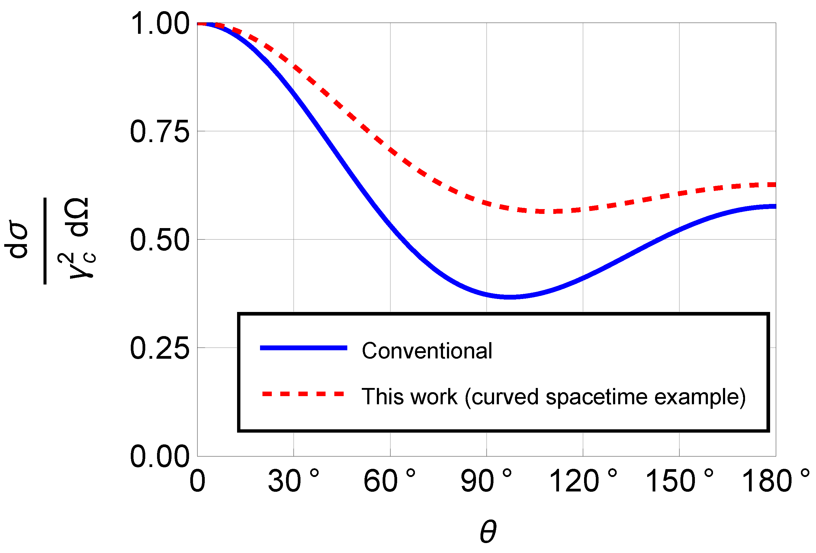
For ${\gamma }_{\mathrm{c}}=0.173$, methods A ($4\times 4$) and B ($256\times 256$ in flat spacetime) exactly agree algebraically, confirming that the proposed matrix representation is strictly consistent with the flat reference.

Method C ($256\times 256$ representation in curved background) is shown as a toy model result under the local-constant-metric (LCM) approximation, using oblique coordinates with constant coefficients (including off-diagonal components). As shown in Figure 1, when visualizing directly with coordinate angle $\theta$, a small deviation appears near $\theta \approx {90}^{\circ }$. This is because off-diagonal metric components change the geometric meaning of coordinate angles, showing that geometric information associated with the chosen coordinate system is reflected in angular dependence.

For methods A and B (flat reference), the differential cross section is:

$${\displaystyle \frac{d\sigma }{d\mathrm{\Omega }}}={\displaystyle \frac{0.125\left(1.45043cos\theta -2.40586\left(3+cos2\theta \right)+0.173cos3\theta \right)}{{\left(-1.173+0.173cos\theta \right)}^3}}.$$

(19)

On the other hand, method C gives

$$\begin{array}{cc}\hfill {\displaystyle \frac{d\sigma }{d\mathrm{\Omega }}}& =5.73001\times {10}^{-20}\left(1.51376\times {10}^{20}-{\displaystyle \frac{3.44859\times {10}^{20}}{1.173-0.173cos\theta }}\right.\hfill \\ \hfill & \left.+{\displaystyle \frac{2.06309\times {10}^{20}}{{(1.173-0.173cos\theta )}^2}}+{\displaystyle \frac{4.62567\times {10}^{18}}{{(1.173-0.173cos\theta )}^3}}\right).\hfill \end{array}$$

(20)

The difference between flat and curved background results demonstrates that this framework has sensitivity to metric geometry.

6. Discussion and Limitations

6.1. Focus of This Work

The main purpose of this paper is to internalize the metric $g_{\mu \nu }\left(x\right)$ into matrices and present the extended Dirac operator

$$D\left(x\right)=i{\widehat{\mathrm{\Gamma }}}_{\nu }\left(x\right){\partial }^{\nu }-m$$

and matrix/trace-based calculation rules. Here

$${\widehat{\mathrm{\Gamma }}}_{\nu }\left(x\right):=\sum _{\mu =0}^3{\mathrm{\Gamma }}_{\mu \nu }\left(x\right),{\mathrm{\Gamma }}_{\mu \nu }\left(x\right):={{\mathrm{\Gamma }}_{\mu }}^{\rho }{g}_{\rho \nu }\left(x\right),$$

and the basis matrices ${{\mathrm{\Gamma }}_{\mu }}^{\nu }$ are constant $256\times 256$ matrices. This paper focuses on the definition and operational rules of this construction; fully curved treatment including connection coefficients and complete position dependence is left for future work.

Note that the indices $\mu ,\nu$ of ${{\mathrm{\Gamma }}_{\mu }}^{\nu }$ are basis labels, not tensor indices, and ${{\mathrm{\Gamma }}_{\mu }}^{\nu }$ itself is a fixed, position-independent matrix (Equation (6)).

6.2. Scope of Applicability

1.

Consistency in flat limit: For $g_{\mu \nu }\to {\eta }_{\mu \nu }$, $D\left(x\right)$ matches the standard $4\times 4$ formalism under unique correspondence via trace normalization. We numerically confirmed exact agreement for tree-level processes including Compton scattering [1,7].

2.

Local-constant-metric (LCM) approximation: When $g_{\mu \nu }\left(x\right)$ varies slowly, approximating $g_{\mu \nu }$ as roughly constant in small regions is possible. Under this approximation, $D\left(x\right)$ is operationally useful, and results from each region can be appropriately weighted to estimate position-dependent effects (the toy model in this paper adopts this stance).

6.3. Computational Advantages

1.

Rules are unified through matrix products and traces, suitable for automation. Implementations can be shared across processes (effective gamma and spin sums → traces).

2.

With trace normalization fixed, direct comparison with flat reference formulas is possible.

3.

Parameter scanning over metric components is easy, enabling reproducible numerical verification.

6.4. Limitations and Future Work

1.

Loop calculations and renormalization: Whether transparency comparable to conventional methods can be maintained while keeping background treatment consistent is a future consideration [3,4].

2.

Position-dependent backgrounds: Beyond the LCM approximation, we plan to implement first-order corrections in perturbative situations like weak gravity or gravitational waves, systematically identifying processes and scales where deviations can appear.

3.

Fully covariant derivatives: Extension to general covariant form including connection coefficients ${{\{}^{\nu }}_{\rho \sigma }\}\left(x\right)$ is needed.

Overall, this method is a practical alternative focusing on presenting the operator and calculation rules. It enables rapid, reproducible calculations based on matrix algebra while maintaining consistency with flat reference formulas.

7. Conclusions

In this work, we defined the extended Dirac operator

$$D\left(x\right)=i{\widehat{\mathrm{\Gamma }}}_{\nu }\left(x\right){\partial }^{\nu }-m$$

using $256\times 256$ two-index gamma matrix representation with metric components internalized into the matrix side. The spacetime dimension remains 4, and geometric information is encoded as matrix coefficients. We also presented calculation rules reducing scattering calculations to matrix products and traces.

In the flat limit, standard results are reproduced under unique correspondence determined by trace normalization. As representative examples, we performed trial numerical verification for Compton scattering in the main text, and for Møller scattering, Bhabha scattering, and muon pair production in the appendices. In the toy model under LCM approximation, we showed that off-diagonal metric components can induce characteristic corrections in the angular dependence of scattering cross sections.

Fully curved treatment, namely general covariant form including connection coefficients ${{\{}^{\nu }}_{\rho \sigma }\}\left(x\right)$

$$D_{\mathrm{cov}}\left(x\right)=i{\widehat{\mathrm{\Gamma }}}_{\nu }\left(x\right)\left({\partial }^{\nu }+{{\{}^{\nu }}_{\rho \sigma }\}\left(x\right)\right)-m$$

is left for future work.

The advantages of this framework are: (i) automation and reproducibility, (ii) direct comparability with flat reference formulas, and (iii) ease of parameter scanning over metric components. Future directions include: systematization under action density including $\sqrt{-g}$, refinement of anticommutation properties of effective gamma ${\widehat{\mathrm{\Gamma }}}_{\nu }\left(x\right)$, introduction of first-order corrections in position-dependent backgrounds (weak gravity, gravitational waves), and examination of loop calculations and renormalization.

Appendix B.1. Minkowski Spacetime Calculation with 4×4 γ Matrices

The unpolarized squared scattering amplitude is given by:

$$\begin{array}{c}\hfill {\left|M\right|}^2={\displaystyle \frac{1}{4}}{\displaystyle \frac{e^4}{q^4}}Tr\left[(\cancel{p}-m){\gamma }^{\mu }(\cancel{p}+m)\right]·Tr\left[(\cancel{\kappa }+M){\gamma }^{\mu }(**\kappa *{*}^{\prime }-M){\gamma }_{\nu }\right],\end{array}$$

(A1)

which in Mandelstam variables becomes:

$$\begin{array}{c}\hfill {\left|M\right|}^2={\displaystyle \frac{1}{8m^2{M}^2}}{\displaystyle \frac{e^2}{s^2}}\left[t^2+u^2+4(m^2+M^2)s-2{(m^2+M^2)}^2\right],\end{array}$$

(A2)

where m and M are the electron and muon masses, respectively. In the high-energy regime of the center-of-mass system ($s\gg m^2,M^2$), masses can be neglected, and the unpolarized amplitude becomes:

$$\begin{array}{c}\hfill {\left|M\right|}^2={\displaystyle \frac{1}{2}}{\displaystyle \frac{e^2}{s^2}}(t^2+u^2).\end{array}$$

(A3)

Using kinematic relations:

$$\begin{array}{cc}\hfill t& ={\displaystyle \frac{1}{2}}s(1-cos\theta ),\hfill \\ \hfill u& ={\displaystyle \frac{1}{2}}s(1+cos\theta ),\hfill \end{array}$$

(A4)

and the differential cross section formula:

$${\displaystyle \frac{d\overline{\sigma }}{d\mathrm{\Omega }}}={\displaystyle \frac{1}{64\pi s}}{\left|M\right|}^2,$$

(A5)

the final result is:

$${\displaystyle \frac{d\overline{\sigma }}{d\mathrm{\Omega }}}={\displaystyle \frac{1}{4}}{\displaystyle \frac{{\alpha }^2}{s}}(1+{cos}^2\theta ),$$

(A6)

where $\alpha =e^2/4\pi$.

Integrating over scattering angle, the total cross section is [1]:

$$\begin{array}{cc}\hfill \overline{\sigma }(e^{-}+e^{+}\to {\mu }^{-}+{\mu }^{+})& ={\displaystyle \frac{4\pi {\alpha }^2}{3s}}=1.33333{\displaystyle \frac{\pi {\alpha }^2}{s}}.\hfill \end{array}$$

(A7)

Appendix B.2. Trial Calculation Using 16 256×256 Effective Matrices Γ ^ in Curved Background

As with the Compton scattering calculation, we adopt the toy metric:

$$g_{\mu \nu }=\left(\begin{array}{cccc}-1& \frac{1}{20}& \frac{1}{10}& 0\\ \frac{1}{20}& \frac{10}{9}& 0& 0\\ \frac{1}{10}& 0& \frac{10}{9}& 0\\ 0& 0& 0& \frac{10}{9}\end{array}\right).$$

(A8)

A representative example obtained with this choice is:

$$\begin{array}{cc}\hfill {\displaystyle \frac{d\overline{\sigma }}{d\mathrm{\Omega }}}& ={\displaystyle \frac{8103617490588876123937{\alpha }^2}{30083573867060726457376s}}\hfill \\ \hfill & -{\displaystyle \frac{371011893098098217579{\alpha }^{2}cos\theta }{15041786933530363228688s}}\hfill \\ \hfill & +{\displaystyle \frac{6196145656745290669593{\alpha }^2{cos}^2\theta }{30083573867060726457376s}}.\hfill \end{array}$$

(A9)

Integrating over $\theta$, the total cross section is:

$$\begin{array}{cc}\hfill \overline{\sigma }(e^{-}+e^{+}\to {\mu }^{-}+{\mu }^{+})& ={\displaystyle \frac{22403380637923042917467\pi {\alpha }^2}{16922010300221658632274s}}\approx 1.32400{\displaystyle \frac{\pi {\alpha }^2}{s}}.\hfill \end{array}$$

(A10)

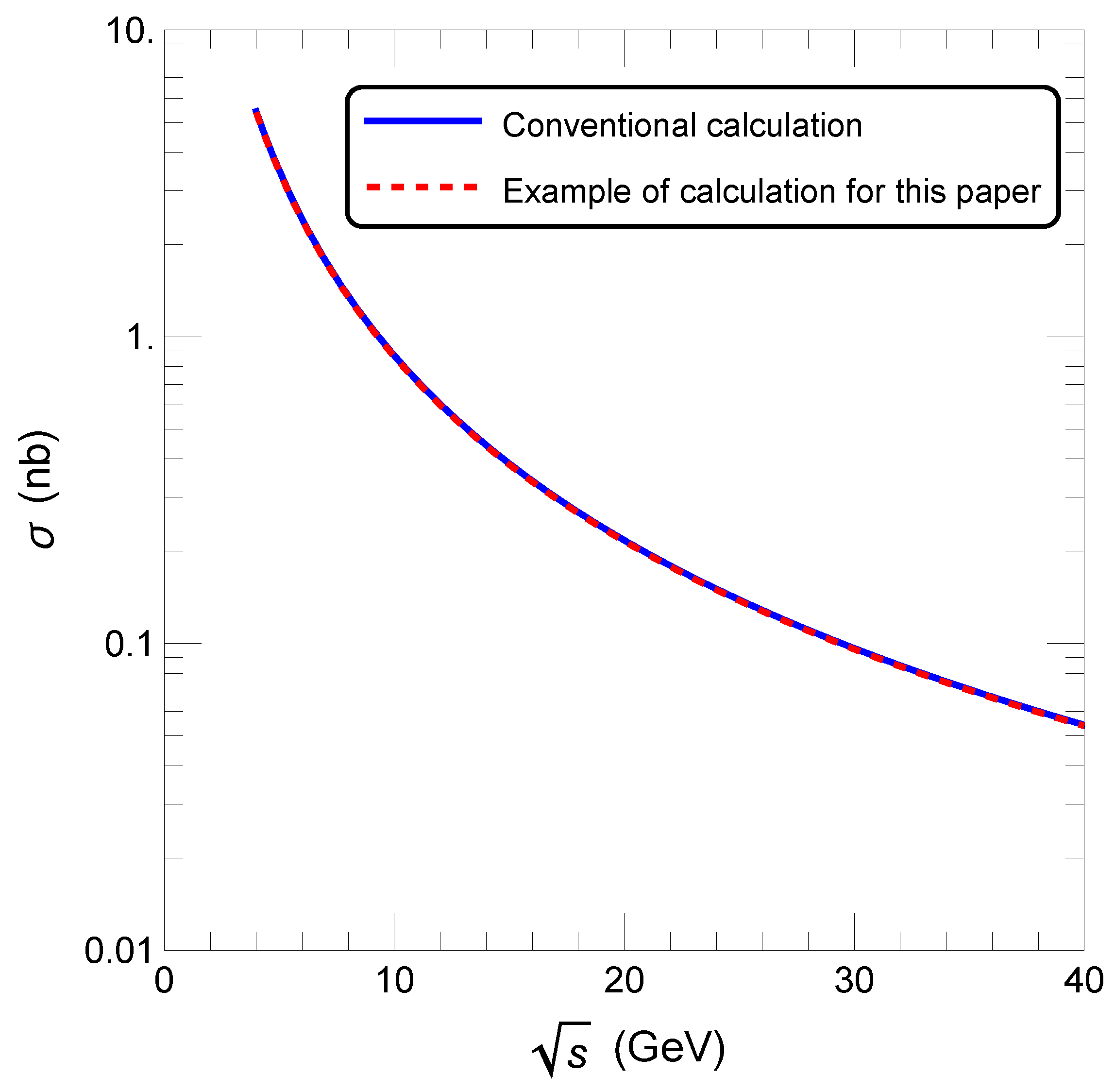
For comparison visualization, both are plotted in Figure A1.

Figure A1 shows that the conventional formula and trial results of this method nearly overlap. This suggests that this process is relatively insensitive to the adopted toy metric. Therefore, even with $e^{+}{e}^{-}$ collision experiments available at accelerators, significant improvement in experimental precision would likely be needed to verify this framework through this process.

Figure A1. Trial example of muon pair production in $e^{+}{e}^{-}$ collisions.

Figure A1. Trial example of muon pair production in $e^{+}{e}^{-}$ collisions.

Appendix C.1. Møller Scattering in Minkowski Spacetime with 4×4 γ Matrices

At leading order, the Møller scattering cross section in Mandelstam variables is

$$\begin{array}{cc}\hfill d\sigma & =dt{\displaystyle \frac{4\pi e^4}{{(s-4m^2)}^2}}[f(t,u)+g(t,u)+f(u,t)+g(u,t)].\hfill \end{array}$$

(A11)

Following [2], the trace expressions are defined as

$$\begin{array}{cc}\hfill f(t,u)& ={\displaystyle \frac{1}{16t^2}}·Tr\left[(**\kappa *{*}^{\prime }+m){\gamma }^{\mu }(\cancel{\kappa }+m){\gamma }^{\nu }\right]·Tr\left[(**p*{*}^{\prime }+m){\gamma }_{\mu }(\cancel{p}+m){\gamma }_{\nu }\right],\hfill \\ \hfill g(t,u)& =-{\displaystyle \frac{1}{16tu}}·Tr\left[(**\kappa *{*}^{\prime }+m){\gamma }^{\mu }(\cancel{\kappa }+m){\gamma }^{\nu }(**p*{*}^{\prime }+m){\gamma }_{\mu }(\cancel{p}+m){\gamma }_{\nu }\right].\hfill \end{array}$$

(A12)

Substituting into Equation (A11):

$$\begin{array}{cc}\hfill f(t,u)& ={\displaystyle \frac{1}{t^2}}\left[{\displaystyle \frac{s^2+u^2}{2}}+4m^2(t-m^2)\right],\hfill \\ \hfill g(t,u)& =g(u,t)={\displaystyle \frac{2}{tu}}\left({\displaystyle \frac{s}{2}}-m^2\right)\left({\displaystyle \frac{s}{2}}-3m^2\right).\hfill \end{array}$$

(A13)

In the ultra-relativistic limit ($p^2\simeq {ϵ}^2$), the differential cross section is [2]

$$\begin{array}{cc}\hfill d\sigma & =r_e^2{\displaystyle \frac{m^2}{{ϵ}^2}}{\displaystyle \frac{1}{4}}{\displaystyle \frac{{(3+{cos}^2\theta )}^2}{{sin}^4\theta }}d\mathrm{\Omega }\hfill \\ \hfill & =r_e^2{\displaystyle \frac{m^2}{{ϵ}^2}}{\displaystyle \frac{1}{16}}{(7+cos2\theta )}^2{csc}^4\theta d\mathrm{\Omega }.\hfill \end{array}$$

(A14)

Appendix C.2. Trial Calculation in Curved Background Using 16 256×256 Effective Matrices Γ ^

Here we show only ultra-relativistic results ($p^2\simeq {ϵ}^2$). Details of derivation are given in Appendix E:

$$\begin{array}{cc}\hfill d\sigma & ={\displaystyle \frac{{\alpha }^2}{71233134002380800000000}}\hfill \\ \hfill & \times (76886835850472311816421\hfill \\ \hfill & +21309289762800530919472cos2\theta \hfill \\ \hfill & +942204894651807977595cos4\theta )\hfill \\ \hfill & \times {csc}^4\theta d\mathrm{\Omega }.\hfill \end{array}$$

(A15)

To facilitate comparison of Equations (A14) and (A15), both are plotted in Figure A2.

Figure A2. Trial example of Møller scattering differential cross section.

Figure A2. Trial example of Møller scattering differential cross section.

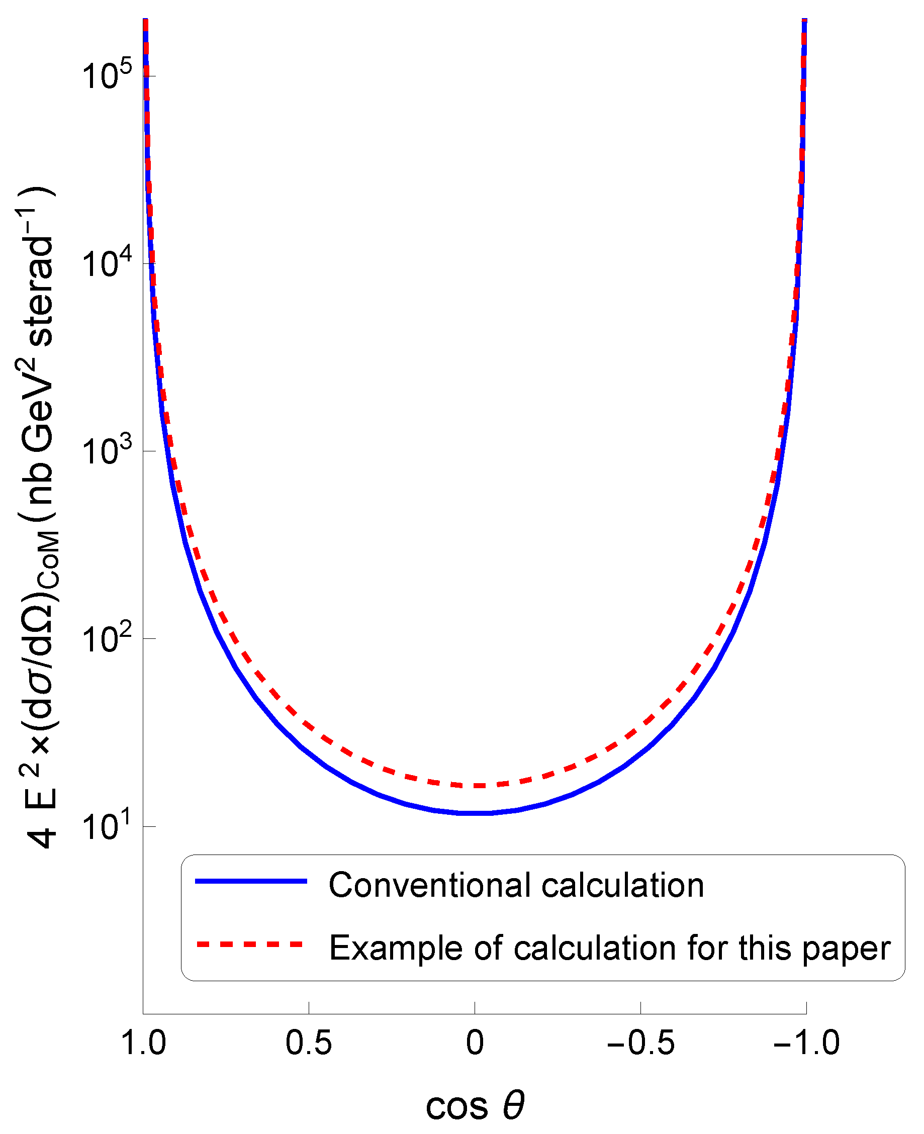
Figure A2 shows that conventional results (solid line) and trial results of this method (dashed line) differ depending on scattering angle, with more pronounced differences in the backward region ($cos\theta \to -1$). This suggests that the metric can influence angular dependence. Experimental verification requires high-precision measurements, but is in principle possible.

Appendix D.1. Bhabha Scattering in Minkowski Spacetime with 4×4 γ Matrices

At leading order for Bhabha scattering, the cross section is obtained by making the substitution $s\to u$ in the denominator of the Møller scattering formula (Equation (A13)).

In the ultra-relativistic limit ($p^2\simeq {ϵ}^2$), the differential cross section is:

$$\begin{array}{cc}\hfill d\sigma & =r_e^2{\displaystyle \frac{m^2}{{ϵ}^2}}{\displaystyle \frac{1}{4}}{\displaystyle \frac{{(3+{cos}^2\theta )}^2}{{sin}^4\theta }}{cos}^4{\displaystyle \frac{\theta }{2}}d\mathrm{\Omega }\hfill \\ \hfill & ={\displaystyle \frac{{\alpha }^2}{256{ϵ}^2}}{(7+cos2\theta )}^2{csc}^4{\displaystyle \frac{\theta }{2}}d\mathrm{\Omega }.\hfill \end{array}$$

(A16)

Appendix D.2. Trial Calculation in Curved Background Using 16 256×256 Effective Matrices Γ ^

We show only ultra-relativistic results ($p^2\simeq {ϵ}^2$). Details are given in Appendix E:

$$\begin{array}{cc}\hfill d\sigma & ={\displaystyle \frac{{\alpha }^2}{569865072019046400000000}}\hfill \\ \hfill & \times (678984214898010488151643\hfill \\ \hfill & -85268530601173881371728cos\theta \hfill \\ \hfill & +193781867538668508561356cos2\theta \hfill \\ \hfill & -587053428853200302960cos3\theta \hfill \\ \hfill & +6196145656745290669593cos4\theta )\hfill \\ \hfill & \times {csc}^4{\displaystyle \frac{\theta }{2}}d\mathrm{\Omega }.\hfill \end{array}$$

(A17)

To facilitate comparison, both are plotted in Figure A3.

Figure A3. Trial example of Bhabha scattering differential cross section.

Figure A3. Trial example of Bhabha scattering differential cross section.

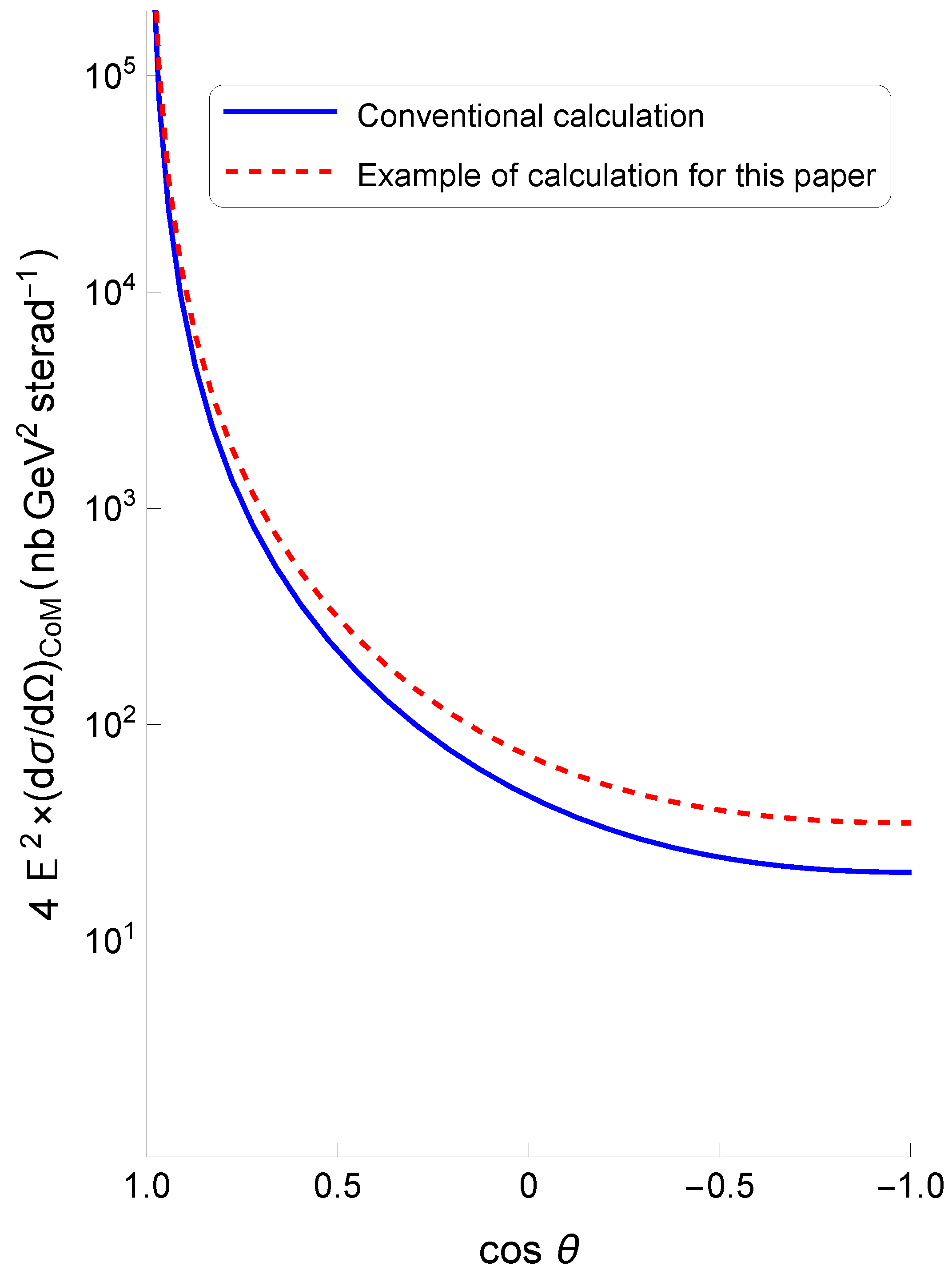
Figure A3 shows angular-dependent differences between conventional results (solid line) and trial results of this method (dashed line), particularly pronounced in the backward region ($cos\theta \to -1$). This suggests that the metric can influence angular dependence. Experimental confirmation requires high precision, but is in principle possible.

References

- Peskin, M.E.; Schroeder, D.V. An Introduction to Quantum Field Theory; Addison–Wesley: Reading, MA, USA; CRC Press eBook, 1995. [Google Scholar] [CrossRef]
- Berestetskii, V.B.; Lifshitz, E.M.; Pitaevskii, L.P. Quantum Electrodynamics, 2nd ed.; Pergamon (Elsevier): Oxford, UK, 1982. [Google Scholar]
- Parker, L.; Toms, D.J. Quantum Field Theory in Curved Spacetime: Quantized Fields and Gravity; Cambridge University Press: Cambridge, UK, 2009. [Google Scholar] [CrossRef]
- Fulling, S.A. Aspects of Quantum Field Theory in Curved Spacetime; Cambridge University Press: Cambridge, UK, 1989. [Google Scholar] [CrossRef]
- Weinberg, S. Gravitation and Cosmology: Principles and Applications of the General Theory of Relativity; Wiley: New York, NY, USA, 1972. [Google Scholar]
- Wald, R.M. General Relativity; University of Chicago Press: Chicago, IL, USA, 1984. [Google Scholar] [CrossRef]
- Klein, O.; Nishina, Y. Über die Streuung von Strahlung durch freie Elektronen nach der neuen relativistischen Quantendynamik von Dirac. Z. Phys. 1929, 52, 853–868. [Google Scholar] [CrossRef]
- Heitler, W. The Quantum Theory of Radiation, 3rd ed.; Oxford University Press: Oxford, UK, 1954. [Google Scholar]
- Bagchi, B.; Ghosh, R.; Gallerati, A. Dirac Equation in Curved Spacetime: The Role of Local Fermi Velocity. Eur. Phys. J. Plus 2023, 138, 1037. [Google Scholar] [CrossRef]
- Arminjon, M.; Reifler, F. Equivalent forms of Dirac equations in curved spacetimes and generalized de Broglie relations. Braz. J. Phys. 2013, 43, 64–77. [Google Scholar] [CrossRef]
- Pollock, M.D. On the Dirac Equation in Curved Space-Time. Acta Phys. Pol. B 2010, 41, 1827–1855. [Google Scholar]
- Sato, H. Groups and Physics; (In Japanese). Maruzen: Tokyo, Japan, 1993. [Google Scholar]
- Lounesto, P. Clifford Algebras and Spinors, 2nd ed.; Cambridge University Press: Cambridge, UK, 2001. [Google Scholar]
- Lawson, H.B., Jr.; Michelsohn, M.-L. Spin Geometry; Princeton University Press: Princeton, NJ, USA, 1989. [Google Scholar]
- Porteous, I.R. Clifford Algebras and the Classical Groups; Cambridge University Press: Cambridge, UK, 1995. [Google Scholar]
- Hestenes, D. Clifford Algebra to Geometric Calculus: A Unified Language for Mathematics and Physics; Reidel (Kluwer): Dordrecht, The Netherlands, 1984. [Google Scholar]
- Doran, C.; Lasenby, A. Geometric Algebra for Physicists; Cambridge University Press: Cambridge, UK, 2003. [Google Scholar]
- Shapiro, I.L. Covariant Derivative of Fermions and All That. Universe 2022, 8, 586. [Google Scholar] [CrossRef]
Figure 1.
Comparison of calculation methods for Compton scattering (). Methods A and B (flat spacetime; and ) exactly agree, serving as the validation benchmark. Method C is a toy model result under the local-constant-metric (LCM) approximation using oblique coordinates with constant coefficients including off-diagonal components. This figure is intended to show (i) the proposed matrix-based calculation rules work correctly, and (ii) sensitivity to coordinate choice can arise; it does not claim direct physical curvature effects.
Disclaimer/Publisher’s Note: The statements, opinions and data contained in all publications are solely those of the individual author(s) and contributor(s) and not of MDPI and/or the editor(s). MDPI and/or the editor(s) disclaim responsibility for any injury to people or property resulting from any ideas, methods, instructions or products referred to in the content. |
© 2026 by the authors. Licensee MDPI, Basel, Switzerland. This article is an open access article distributed under the terms and conditions of the Creative Commons Attribution (CC BY) license (http://creativecommons.org/licenses/by/4.0/).
Copyright: This open access article is published under a Creative Commons CC BY 4.0 license, which permit the free download, distribution, and reuse, provided that the author and preprint are cited in any reuse.