
Submitted:
07 January 2026
Posted:
07 January 2026
You are already at the latest version
Abstract
Shapley values are the most widely used point-valued solution concept for cooperative games and have recently garnered attention for their applicability in explainable machine learning. Due to the complexity of Shapley value computation, users mostly resort to Monte Carlo approximations for large problems. We take a detailed look at an approximation method grounded in multilinear extensions proposed by Okhrati and Lipani (2021) under the name Owen sampling. We point out why Owen sampling is biased and propose unbiased alternatives based on combining multilinear extensions with stratified sampling and importance sampling. Finally, we discuss empirical results of the presented algorithms for various cooperative games including real-world explainability scenarios.
Keywords:
cooperative game theory
; multilinear extensions
; importance sampling
; stratified sampling
; Shapley value
1. Introduction
Cooperative game theory [1] models situations where entities (players) collaborate to achieve a common objective. Example scenarios (games) include voting situations in parliaments [2,3,4], sharing of infrastructure costs [5,6,7] or the analysis of genetic networks [8,9]. More recently, cooperative game theory has garnered plenty of interest in the field of explainable artificial intelligence (XAI) and interpretable machine learning [10,11,12,13], where the players are the features of a machine learning model contributing to a certain prediction. In each case, cooperative game theory provides tools — primarily in the form of point-valued solution concepts — to analyze how the total benefit or cost resulting from cooperation should be fairly distributed between the participating players. Among these, the Shapley value [14] is both the most widely used point-valued solution concept in classical cooperative game theory applications and the predominant game theory based tool in XAI.
For n players, there are coalitions in a cooperative game. Calculating the Shapley value of a general cooperative game exactly was shown to be NP-hard [15,16,17]. Various concepts for approximating Shapley values for large n have been proposed — far too numerous to even attempt listing them all in this introduction — with plenty of recent approaches sparked by the desire to employ Shapley values for determining the significance of features with respect to the outcome of neural networks [10,11,12,13]. In our view, the large variety of approximation algorithms is at least partly due to the fact that the methods are tailored to specific formulations of the Shapley value, which can be expressed in several mathematically equivalent ways. For example, the Shapley value can be regarded as an average over permutations [18], as the optimal solution to a least squares problem [19], as a weighted sum over coalitions [14] or as an integral of the game’s multilinear extension [20].
To overcome this fragmentation, Benati et al. [21] proposed a unified framework as a “stochastic approach to approximate values in cooperative games”. In detail, their work defines a general approach for estimating linear solution concepts, a subclass of point-valued solution concepts including the Shapley value, via Monte Carlo methods. We extend their approach by introducing a novel connection to importance sampling, i.e., a variance reduction technique for Monte Carlo methods, thereby providing a stronger theoretical foundation for their framework as well as promoting it — since, as for our for our knowledge this article is the first work applying the ideas from [21] in XAI. Building on this connection, we show that several well-known approximation algorithms for the Shapley value, in particular some of those based on multilinear extensions, fit into this framework. This unifying perspective enables a more systematic comparison of algorithms, leading to new insights and recommendations for choosing among different approximation methods.
Importantly, the goal of this paper is neither to propose any completely novel approach for estimating Shapley values nor to perform comparisons over a range of approximation algorithms. Rather, beyond the importance sampling framework on the coalition space mentioned in the previous paragraph, we also provide structural and algorithmic insight into very widely used methods for computing Shapley values based on multilinear extensions. Specifically, we take a closer look at an algorithm originally called Owen sampling (OS) published by Okhrati and Lipani in 2021 [22], which, according to Google Scholar on Dec. 31, 2025, was already cited 76 times. The seminal paper Chen et al. [12] reports that OS is biased, but does not give a formal proof or perform a detailed numerical investigation into the bias. Further, Chen et al. [12] sketch an unbiased version for multilinear extension sampling while conceding that the biased approach may be more common as it improves convergence and later briefly mentioning in one sentence that their unbiased version was equivalent to sampling appropriately from the coalition space. This paper fills the theoretical and algorithmic gaps by
- establishing the bias in the original algorithm from [22] formally and confirming it in numerical experiments,
- formally specifying and analyzing the unbiased version for multilinear extension sampling sketched in [12] and pointing out its equivalence to a weighted sampling strategy on the coalition space rigorously using the aforementioned importance sampling framework and
The paper is organized as follows. In Section 2, we introduce the basic ideas from cooperative game theory, including linear solution concepts and the Shapley value, whereas Section 3 provides a brief introduction to Monte Carlo methods as well as importance sampling and stratified sampling for variance reduction. We establish a novel framework for importance sampling on the coalition space for linear solution concepts based upon Benati et al. [21] in Section 4. The core of the paper follows in Section 5. We introduce and develop unbiased sampling algorithms based on multilinear extensions. Using these algorithms and the importance sampling framework from Section 4, we then derive new algorithms, which are closely related to the multilinear-extension-based algorithms, employing similar distributions and incorporating analogical architectures including sample reuse across players. We offer coalition-based sampling algorithms with more favourable properties than the multilinear-extension-based concepts from [12,22]. In Section 6, we analyze the performance of the algorithms from Section 5 empirically for two different types of cooperative games as well as three real-world XAI applications and confirm the claims from our previous analysis numerically. We end with a summary, our conclusions and some recommendations in Section 7.
2. Preliminaries on Cooperative Game Theory
This section provides a brief introduction to cooperative games with transferable utility and point-valued solution concepts such as the Shapley value along the lines of the two textbooks by Chakravarty et al. [1] and by Peters [23] as well as the research paper by Benati et al. [21].
2.1. Transferable Utility Games and Their Characteristic Functions
In this work, we study transferable utility games (TU games), which are cooperative games satisfying the restriction that the earnings of a coalition can be expressed by a scalar [1,23]. This comes with the implicit assumption that this value — the amount of utility — can be freely distributed and transferred among players.
Following the definitions in [1,23], a TU game is formally given by a pair with being the set of players and being the characteristic function defined on the subsets of N. The characteristic function v assigns a real value to each coalition that represents its total utility when its members cooperate. We always follow the normalization .
It sometimes proves to be convenient to identify a coalition S with an indicator vector . Thus, we define , and, conversely, . Under this mapping, all functions and operators defined on either or are implicitly also defined on its counterpart, e.g., and are used interchangeably and is equivalent to .
2.2. Linear Solution Concepts for TU Games
Let be the set of TU games with player set N. A point-valued solution concept is a map that assigns a vector to each game . Each element of that vector denotes the worth of player i according to the underlying solution concept. In general, point-valued solution concepts are used when the influences of players need to be measured, or when the payoff of a coalition of cooperating players needs to be allocated between the members of S.
A desirable property of a solution concept is linearity [21], which means that can be written as
with ⊙ being the Hadamard product of vectors, being weights depending only on S and the player, and being values depending on S, v, and the player.
2.3. The Shapley Value
The Shapley value [14] is the most prominent solution concept for TU games. Recently, it received plenty of attention in the context of machine learning and explainable artificial intelligence [10,11,12]. For each player , its Shapley value is defined as the expected marginal contribution to the set S of all players before player i in a random permutation of N, i.e.,
where denotes a uniform distribution, is the set of all permutations of N, and returns the set of all players before player i in a given permutation . Note that we will write as long as the characteristic function v is clear from context.
The vector of all players’ Shapley values is given by , and any approximation thereof is denoted by , with its i-th component given by . As long as there is no ambiguity, we will write .
Clearly, via (3), one obtains that the Shapley value fits into the framework of linear solution concepts defined in Section 2.2, with the individual elements of being defined as
and .
2.4. The Banzhaf Value
The Banzhaf value [24,25] is another prominent point-valued solution concept for TU games. In the fields of machine learning and artificial intelligence, it can be regarded the second most important solution concept from cooperative game theory [26,27]. For a player , the Banzhaf value is defined as the expected marginal contribution of i to a random coalition, i.e.,
with denoting the uniform distribution and being the marginal contribution of i to S, as in the previous subsection. The vector of all players’ Banzhaf values is given by . Similar to the Shapley value, the Banzhaf value also fits into the framework of linear solution concepts from Section 2.2, with the individual components of being defined as
and .
3. Preliminaries on Monte Carlo Methods for Estimation
In this section, we give a brief introduction to the application of Monte Carlo methods for estimating expectations. We mostly follow the two short overviews provided by Rubinstein and Kroese [28] and by Botev and Ridder [29].
Let be a discrete (or continuous) d-dimensional random variable taking values from and following a known or unknown probability mass function (or probability density function, respectively). Furthermore, let represent a concrete realization of . For a given function , our goal is to estimate
For many practical problems, this expectation cannot be computed in closed form, because often itself is unknown (we only have i.i.d. samples, e.g., in the form of observations or measurements), or because the sum (or integral, respectively) defining the expectation is intractable to compute. In the latter case, Monte Carlo methods replace the analytical challenge by simulation.
We start by introducing the crude Monte Carlo method, which is the simplest approach, followed by two variance reduction techniques studied in this paper. We emphasize that we always assume finite variances of throughout this article.
3.1. Crude Monte Carlo Method
When using the Crude Monte Carlo method, a sample of size is drawn, and is approximated by averaging all . Thus, Botev and Ridder [29] define an estimator of as
Furthermore, one can easily obtain via Chebyshev’s inequality [31] that is consistent in probability, i.e., for all , there holds
3.2. Importance Sampling for Variance Reduction
Following the introductions of importance sampling in [28,30], we provide a brief unified treatment that covers both discrete and continuous probabilities.
In the context of importance sampling, another probability mass function (or probability density function, respectively) with is introduced, such that (6) can be rewritten as
Based on (9), a Monte Carlo approximation is given by
with . The resulting estimator is unbiased [28], i.e.,
and clearly, as for the crude Monte Carlo method, its variance is given by
As long as is properly selected, the variance of the estimator is always less or equal compared to the variance of the crude Monte Carlo estimator from Section 3.1. This can easily be seen by comparing (8) and (12), resulting in
which always holds since one could always choose in the worst case.
The importance sampling estimator is also consistent in probability, which can be confirmed via Chebyshev’s inequality [31]. For all , there holds
3.3. Stratified Sampling for Variance Reduction
Stratified sampling [29] is a well-known variance reduction technique for Monte Carlo methods. It partitions the sample space into ℓ disjoint strata such that with for . Let L be a discrete random variable taking values from with known probabilities . Then, can be rewritten as
with being the expectation over the conditional probability distribution of given that . Based on this formulation of , one obtains an estimator of as
where is the estimated value of in stratum , i.e.,
and the sample of size is drawn i.i.d. from the conditional probability distribution of given that . To allow for fair comparisons to other Monte Carlo techniques, we always assume (up to some rounding errors), where denotes the overall sample budget. The resulting estimator is unbiased [29], i.e.,
and its variance is discussed in the following. Unlike in the previous subsections, our goal here is not to simply define the variance of the estimator, but instead to derive it in order to understand its origins. This deeper understanding will be crucial for our subsequent analysis in Section 5.
For the two random variables and L defined earlier, Eve’s law [31], also referred to as the law of total variance or the variance decomposition formula in the literature, states
and therefore, by using (8), the variance of the crude Monte Carlo estimator from Section 3.1 is given by
Since the individual estimators are independent, the variance of the estimator based on stratified sampling is given by
Once we assume that the sample sizes per stratum are proportionally assigned, i.e., , Equation (17) simplifies to
Therefore, by comparing the variance from (18) to the variance of the crude Monte Carlo estimator given in (16), it is easy to obtain that the variance of the stratified estimator is always less or equal compared to that of the crude Monte Carlo estimator, as long as the stratum sample sizes are proportionally assigned with respect to , see also [29]. In detail, we highlight that stratification removes the variance of the expectations between strata, i.e., the non-negative term in (16) vanishes.
For completeness, we note that the strata sample sizes which minimize the variance of the overall estimator [29] are given by
Since in most settings the standard deviations are not known, one might use two-stage algorithms that use pilot runs in the first stage to approximate all and calculate the final sample sizes via (19) based on those .
Concluding this subsection, we note that the estimator obtained via stratified sampling with a sample allocation proportional to is consistent in probability, which can again be shown via Chebyshev’s inequality [31]. For all , there holds
4. An Importance Sampling Framework for Linear Solution Concepts and Marginal Contribution Importance Sampling for the Shapley Value
Calculating the value of a linear solution concept, i.e., (1), exactly usually requires summing up or terms. Thus, approximation approaches are needed to estimate these values in real-world scenarios. The latter statement is particularly relevant in the context of applications in explainable artificial intelligence [10,11,12,13] where one can frequently not exploit any special structure of the underlying game in order to compute Shapley values exactly. In the following two subsections, we revisit some ideas from Benati et al. [21] and present them in a general framework for importance sampling on the coalition space for linear solution concepts. We first introduce the crude Monte Carlo method on the coalition space based on the uniform sampling strategy from [21]. Afterwards, we develop our general importance sampling framework for approximating linear solution concepts and point out that the weighted sampling strategy for estimating the Shapley value from (3) introduced in [21] can be regarded as marginal contribution importance sampling.
4.1. Crude Monte Carlo Method on the Coalition Space
Benati et al. [21] discuss a uniform sampling strategy on the coalition space. We will in this work consider it as the crude Monte Carlo method on the coalition space.
First, by reformulating (1) for a specific player , we obtain
with being a uniform distribution over all subsets, i.e., .
Thus, a simple approximation of (1) via the crude Monte Carlo method in a sense of (7) is given by generating a sample of size with , and, based on that, calculating
Note that throughout this work, we use S to denote subsets in general, while sampled subsets are denoted by .
We emphasize that using the uniform distribution over all subsets, q, is the most natural and simplest choice for the crude Monte Carlo approximation of (1), since more sophisticated probability distributions are not justified in this setting. Now, one might ask why the weights cannot be interpreted as probabilities of different coalitions forming, and therefore, serve as the initial underlying distribution that defines the distribution for the crude Monte Carlo method. For instance, for the well-known formulation of the Shapley value given by (3), which follows directly from the assumption that all player permutations are equally likely as defined in (2), these weights indeed can be interpreted as the probability of a subset forming. However, this is not the case for all formulations of the Shapley value, and certainly not for all linear solution concepts [21]. Thus, in general, we cannot use as q in (20).
With that in mind, one might argue that any valid probability distribution (other than the uniform distribution over subsets) could be used in (20), with the inner expectation adapted accordingly, which would also be mathematically correct. However, TU games as introduced in Section 2.1 are specified only by the tuple and do not include any probabilities for the formation of any specific coalitions. (Note in passing that different solution concepts may account for the latter. For example, the Banzhaf value introduced in Section 2.4 assumes that each coalition is equally likely, while the Shapley value introduced in Section 2.3 assumes that each permutation is equally likely, which implies a non-uniform distribution over coalitions.) Therefore, since there is no basis for assigning specific probabilities to different coalitions, we adopt the uniform distribution as a natural and straightforward choice for our crude Monte Carlo method, providing a reasonable starting point for all linear solution concepts.
Readers familiar with the ApproShapley algorithm [18] might think of ApproShapley as the crude Monte Carlo method for approximating the Shapley value contradicting our results above. However, the ApproShapley algorithm addresses a different formulation, i.e., the permutation-based definition of the Shapley value given by (2), where the sampling space is given by all permutations of N. In contrast, when the Shapley value is expressed within the coalition-based framework of linear solution concepts as in (1), and the only requirement is that , the appropriate crude Monte Carlo approximation — based on our previous arguments — is given by sampling according to the uniform distribution over all coalitions and approximating .
4.2. Importance Sampling on the Coalition Space
In the previous subsection, we focused exclusively on sampling subsets from the uniform distribution. While this approach is simple and unbiased, it is not necessarily optimal for all linear solution concepts or problem settings. For example, when computing the Shapley value using (3), small or large coalitions tend to have larger weights. Thus, despite having a strong influence on the estimator, they may retrieve only a few samples when sampling uniformly from the coalition space, potentially reducing the accuracy of the estimator.
To address this issue and enable more efficient sampling schemes, we now consider the use of importance sampling introduced in Section 3.2 as a variance reduction technique. By appropriately reweighting the estimator, importance sampling allows drawing subsets from a non-uniform, user-defined distribution, while still providing an unbiased estimator of the underlying linear solution concept.
Theorem 1.
For all , let
be a probability distribution and with be a sample of size τ generated by sampling with replacement according to . Then,
is an importance sampling estimator of the linear solution concept .
Proof.
In the following, without loss of generality, we fix one player to simplify notations.
First, recall the formulation of linear solution concepts via the uniform distribution over coalitions denoted by q, as defined in (20). Now, we define
which simplifies to . This serves as our new sampling distribution, and it clearly satisfies the requirements for a sampling distribution in the context of importance sampling as specified in Section 3.2. Then, based on (9), we derive
Now, via (10), one obtains
as the importance sampling estimator of as long as . □
The following proposition relates our importance sampling estimator from Theorem 1 to a result from Benati et al. [21], p. 95.
Proposition 1.
The importance sampling estimator from Theorem 1 has the following properties:
- (a)
- It is unbiased, i.e.,
- (b)
- Its variance is given by
- (c)
- It is consistent in probability, i.e.,
Proof.
The proof is straightforward. (22) directly follows from (11), while (24) can be obtained from (13).
□
Remark 1.
It is worth noting that the results from Theorem 1 and Proposition 1 implicitly cover the crude Monte Carlo method from Section 3.1 (and Section 4.1, respectively) by setting . Additionally, it also covers stratified sampling from Section 3.3. Clearly, each individual stratum estimator of a linear solution concept can be brought into the form of (21) and treated as an estimator of an individual linear solution concept, which allows for applying the results from Theorem 1 and Proposition 1.
We note that the goal of our results in this subsection is not to perform better than algorithms tailored to specific solution concepts. Instead, our results provide a general framework that is theoretically grounded in importance sampling on the coalition space, which allows for employing any suitable sampling distribution to approximate any linear solution concept from cooperative game theory. Furthermore, as stated in Remark 1, our approach implicitly covers the crude Monte Carlo method as well as stratified sampling, making it even more general.
Let us finally define a special class of importance sampling algorithms, which we call marginal contribution importance sampling algorithms. As the name suggests, these algorithms approximate linear solution concepts by sampling marginal contributions via importance sampling. Thus, all algorithms that admit the form proposed in Theorem 1 with belong to this class.
A simple estimator named MCIS belonging to the class of marginal contribution importance sampling algorithms for approximating the Shapley value of player i is given by
with given by (4) and , whereby
is the sampling distribution. Note that we can use as the sampling distribution since and . Thus,
We will revisit and further analyze the MCIS estimator for the Shapley value in Section 5.6. We finally note that MCIS estimator for the Shapley value derived via (25), (26) and (27) was discussed in Benati et al. [21], p.96, under the name weighted sampling strategy. We end this section by stressing that the least squares strategy for Shapley values which is promoted and analyzed in detail in the article by Benati et al. [21], is covered by Theorem 1 and Proposition 1. While any approximations based on the least squares formula for the Shapley value are beyond the scope of this manuscript, our key takeaways are both the generality of our importance sampling framework and the relevance of the specific representation of the Shapley value for its Monte Carlo estimation.
5. Multilinear Extensions for Approximating Shapley Values and Connections to Importance Sampling on the Coalition Space
This section covers the idea of multilinear extensions of cooperative games and how this formulation of games can be used to approximate Shapley values of cooperative games. First, we provide a definition of multilinear extensions in Section 5.1 and a representation of the Shapley value in their context in Section 5.2. Afterwards, in Section 5.3, we discuss an existing multilinear-extension-based approximation algorithm for the Shapley value which goes by the name Owen Sampling, was introduced in Okhrati and Lipani [22] and is frequently applied in XAI applictions. Although it was previously noticed that Owen Sampling is biased, e.g. in [12], we are the first to provide a detailed analysis of the bias. Then, we propose unbiased multilinear-extension-based algorithms in Section 5.4 and Section 5.5, with the latter subsection offering a stratified variant. These two unbiased multilinear-extension-based approaches serve as intermediary results for our investigations on the relations to our importance sampling framework on the coalition space from Section 4.2. We discuss our results, conclusions and recommendations in the subsequent Section 5.6 and Section 5.7.
5.1. Definition of Multilinear Extensions
Multilinear extensions have been proposed by Owen [20]. The idea is to extend the characteristic function of a cooperative game, v, which is defined on the subsets of N, to the unit n-hypercube by the function f. As mentioned in Section 2.1, v is implicitly defined on . Based on that formulation, Owen [20] extended the domain to and defined the extension of v as
It is easy to see that this function coincidences with v at the corners of the hypercube, i.e., for all , which means that f is indeed an extension of v. Furthermore, f is linear in each variable, i.e., multilinear, hence the name multilinear extension. We note that Owen [20] showed that f as defined in (28) is the unique multilinear extension of v.
Furthermore, Owen [20] highlighted that f can be thought of as the expected value of v when each player i joins the coalition with their respective probability , i.e.,
whereby is the Bernoulli distribution with probabilities . Note that all elements of are mutually independent events and are obtained via for all .
5.2. The Shapley Value in the Context of Multilinear Extensions
In the setting of multilinear extensions, Owen [20] provided a definition of the Shapley value as
with being the all-ones vector and
This formulation can also be interpreted as the expected marginal contribution of player i when all other players join the coalition with probability , i.e.,
where ⊙ denotes the Hadamard product of vectors, and with being the i-th standard basis vector. Note that means sampling each except the i-th component, which is forced to be 0, such that player i is explicitly excluded.
5.3. Owen Sampling (OS) for Computing Shapley Values According to Okhrati and Lipani
Since calculating (30) or (31) exactly requires evaluations of v, multilinear extensions cannot be used as an exact computation method for large n when no a priori knowledge about the characteristic function is given, but instead serve as a starting point for the development of new approximation algorithms.
In this section, we introduce the OS algorithm proposed by Okhrati and Lipani [22]. To avoid confusion, we highlight that the name of this algorithm is based on Guillermo Owen, who published the idea of multilinear extensions of games [20,25] and defined the Shapley value in this setting [20]. In particular, we emphasize that the algorithm is not related to the Owen value [32], a solution concept for cooperative games with a priori unions.
Okhrati and Lipani [22] approximate (29) by
with being the discretization level. Note in passing that, contrary to the original algorithm in [22], we adjusted the upper bound of the sum in (32) from Q to to ensure that the sum includes exactly Q terms, rather than . Our adjustment is consistent with the source code provided with the original paper [22] which is publicly available via
Since calculating exactly in (32) requires summing over all subsets , the authors approximate (31) by
whereby denotes the k-th sampled vector that is drawn according to the distribution from (31) with all probabilities for being , i.e., . hereby is an additional parameter of the algorithm that specifies the number of evaluations per q. Okhrati and Lipani [22] fixed for all .
It has been shown in the original paper Okhrati and Lipani [22] that this estimator is consistent, i.e., for any and . Unfortunately, Okhrati and Lipani [22] did not include a theoretical investigation of bias or variance. The bias of OS is discussed in [12], where the authors concluded that OS is biased without giving a formal proof. We provide the latter in
Proposition 2.
The OS estimator is biased, i.e., does not hold in the general case.
Proof.
Let us fix an arbitrary player whose Shapley value we want to estimate. We state that (32) does not provide an unbiased approximation of (29), resulting in a biased estimator . To see this, consider the case , where samples are drawn from , , and , such that we have
Clearly, the last equality does not represent a valid relationship between the Shapley value and the Banzhaf value. E.g., consider a game with players and the characteristic function
such that the Shapley values are given by
Then, we obtain
□
Proposition 2 establishes that the OS estimator is biased. (Formally, one might argue that Proposition 2 establishes the existence of a bias for the case by counterexample. Although our proof is specific to this setting, the form of the OS estimator indicates that the bias persists for any finite Q, see also the numerical results in [12]). The origin of that bias can be observed by visualizing the expected number of sampled coalitions per coalition size across different values of Q, as illustrated in Figure 2. Clearly, as Q increases, the expected number of samples per coalition size approaches an equal distribution, as required by the Shapley definition. However, for the two finite values of Q shown in Figure 2, this equal distribution is never fully reached.
Additionally, we refer to Figure 3 in Section 6, which empirically validates the existence of a bias when executing OS.
Due to its biasedness, OS does not fit into the importance sampling framework defined by Theorem 1 since estimators of that framework are unbiased, see Proposition 1. Thus, we cannot use (23) to calculate the variance of OS. As a solution, we propose an unbiased variant of OS in Section 5.4, for which we will calculate the variance.
Algorithm 1 implements (34) as a ready-to-use algorithm with some enhancements. When approximating the Shapley value of all players, these additional improvements reduce the number of evaluations of v, and thus, increase convergence. In detail, by looking at Algorithm 1, one obtains that evaluations of can be reused to update the Shapley value of each individual player, either as the minuend, if player i is already included in the sampled coalition, or as the subtrahend, if excluded. Note that we force the exclusion of player i in the subtrahend to avoid adding marginal contributions of zero. This approach reduces the number of evaluations of the characteristic function per iteration in line 3 from to . We use this implementation when comparing variances and convergence speeds in Section 6.2.
| Algorithm 1:OS |
|
Concluding this subsection, we highlight two more details. First, we note that approximations of the integral in (29) other than (32) have also been proposed. Mitchell et al. [33] mentioned that they used the trapezoidal rule in their implementation of OS. On the other hand, Chen et al. [12] mentioned that sampling at random to approximate (29) provides an unbiased estimator. While we assume the former variant to be biased as well, we will further study the latter approach in Section 5.4.
Second, another algorithm proposed by Okhrati and Lipani [22] called halved Owen sampling uses antithetic sampling as a variance reduction technique [12,28,34]. However, this method lies outside the scope of our paper. Similar to the OS estimator, the halved Owen sampling estimator remains biased. Rather than extending all following developments like the construction of an unbiased variant of OS to the antithetic case as well, we focus exclusively on the OS estimator. From the results of this paper, one could easily derive unbiased or stratified antithetic versions of OS. We refer to [34] for more details on how unbiased antithetic variants of existing algorithms can be constructed.
5.4. Multilinear Extension Sampling for the Shapley Value (MES)
As discussed in the previous subsection, the OS estimator is biased, which motivates the introduction of two new unbiased variants of the estimator in this and the following subsection. Chen et al. [12] proposed an algorithm called random q as an alternative to OS. The idea is to sample points across the interval at random, resulting in an unbiased estimator of the integral in (29) even for small sample sizes. Although the authors refer to this algorithm at several points in their work, Chen et al. [12], do not provide any theoretical analysis of their algorithm. This lack of theoretical grounding motivates a closer examination of random q along with its advantages and limitations in comparison to other approaches.
From now on, we refer to this algorithm as MES (for Multilinear Extension Sampling). In our implementation, we fix due to the fact that we fail to see any justification in [22] to set . In particular, the authors stated in [22] that the optimal choice of is yet to be explored. In our opinion, there is no clear reason why the algorithm benefits from sampling more than one coalition for a given, sampled q. Therefore, our proposed algorithm is controlled by one parameter only, which specifies the number of random draws of q and thus, implicitly, the number of sampled coalitions. The overall number of evaluations of v is then given by .
Proposition 3.
The MES estimator is unbiased, i.e., .
Proof.
Let us fix an arbitrary player whose Shapley value we want to estimate. The sampling procedure of Algorithm 2 is equivalent to sampling . Therefore, we obtain the estimator
where denotes the k-th sample obtained by first drawing at random, and then sampling .
Now, let denote a random variable that is uniformly distributed across with density and concrete realizations . Then,
whereby the closed-form solution of the integral directly comes from the beta function [35,36]. Note that we implicitly switched from vector notation to set notation in the step between (36) and (37), as described in Section 2.1. □
| Algorithm 2:MES |
|
Empirical data given in Figure 3 in Section 6 supports the claim that MES is unbiased. Additionally, it is worth noting that MES may perform worse than OS, as shown in Figure 5, Figure 6, Figure 7, Figure 8 and Figure 9. We attribute this observation to the fact that OS generates its q-values systematically, which probably helps reduce its variance. Although we will later derive a theoretical variance for the MES estimator (see Corollary 1), we cannot compare it to OS since a theoretical variance analysis for OS has not been performed yet.
5.5. Stratified Multilinear Extension Sampling for the Shapley Value (S-MES)
In order to reduce the variance of MES without reintroducing a bias, we propose a new algorithm which splits the interval into strata, such that the strata are defined as
hence its name S-MES. To avoid confusion, we highlight that the strata are defined on the interval space, not on the subset space. As we demonstrate in Section 5.7, these are different stratification schemes.
In each stratum from (38), a random value is drawn uniformly, which serves as the basis to generate a new random coalition based on the Bernoulli distribution . Again, similar to MES from the previous section, S-MES is controlled by one parameter only, which defines the number of sampled coalitions. The total amount of evaluations of v is then given by .
Proposition 4.
The S-MES estimator is unbiased, i.e., .
Proof.
Let us fix an arbitrary player whose Shapley value we want to estimate. The sampling procedure defined in line 4 of Algorithm 3 is equivalent to sampling . Therefore, we obtain the estimator
where denotes the k-th sample obtained by first drawing , and then sampling .
Now, let us denote by random variables that are uniformly distributed across with concrete realizations and densities whenever . Then,
Since the last formula is identical to (36), the rest of the proof proceeds exactly as in Proposition 3 and is therefore omitted here. From there, we obtain
□
| Algorithm 3:S-MES |
|
Again, we refer to Figure 3 in Section 6, which validates the unbiasedness of S-MES empirically. Additionally, Figure 5, Figure 6, Figure 7, Figure 8 and Figure 9 in Section 6 indicate that the variance was reduced compared to MES and appears to be very similar to that of OS, at least in the context of the exemplary games.
Note that we do not derive a theoretical variance for S-MES, but instead propose an improved variant in Section 5.7, for which we will provide the theoretical variance.
5.6. Comparison of MES and Marginal Contribution Importance Sampling (MCIS)
Let us revisit the marginal contribution importance sampling (MCIS) approach for the Shapley value defined by (27), which we introduced at the end of Section 4.2 in the context of our importance sampling framework on the coalition space. We observe
Theorem 2.
MES is the same importance sampling estimator as MCIS.
Proof.
Per definition, MCIS is an importance sampling estimator.
Now, let us fit the MES algorithm into the importance sampling framework from Theorem 1. From (35), one obtains that it is based on marginal contributions as well, such that we have .
Furthermore, from (35), we retrieve , if . For the case , we derive
whereby the last equality directly follows from the proof of Proposition 3, which is why we omit any intermediate steps here.
Since MES updates the estimator by adding with factor 1 (see Algorithm 2), we have , and thus, .
As a result, via (26), one obtains and that completes the proof. □
Proposition 5.
The variance of the MCIS estimator is given by
Proof.
The proof is straightforward by inserting , , and into (23). □
Corollary 1.
The variance of the MES estimator is given by
Proof.
The proof is straightforward taking into account that MES is the same estimator as MCIS (see Theorem 2) and the variance of MCIS is given by Proposition 5. □
We conclude: MCIS is unbiased, which can be obtained directly from Proposition 1 since MCIS belongs to the importance sampling framework defined by Theorem 1, and MES is unbiased, see Proposition 3. Additionally, via Proposition 5 and Corollary 1, we see that both algorithms share the same variance. As a result, we argue that the indirection introduced by Algorithm 2, i.e., sampling from the multilinear extension of v, does not have any advantages over sampling directly from the coalition space with probabilities .
We refer to Section 6, where Figure 4 validates the proposed variances from Proposition 5 and Corollary 1.
To allow fair comparisons to other algorithms, we reuse evaluations of v across players, as for all other algorithms. We refer to Algorithm 4 for a ready-to-use implementation of this improved variant, where the number of evaluations of v is given by and
is the adapted sampling distribution to achieve this improvement.
Proposition 6.
Proof.
When sampling according to (39), i.e., , the probability of sampling a subset of size that can be used to update (27) is given by
From (40), we obtain that each coalition size without player i is equally likely, as in (26). Furthermore, from (39), we see that each coalition has the same probability within equal-sized coalitions, such that sampling according to (39) in Algorithm 4 is indeed equivalent to (26). That completes the proof. □
| Algorithm 4:MCIS |
|
We acknowledge that Chen et al. [12] already observed that MES is equivalent to sampling coalitions according to (26), which aligns with our Theorem 2. This, however, does not diminish the novelty of our contribution. First, we establish MES within the general importance sampling framework proposed in Theorem 1. Second, the results in this subsection serve only as intermediate steps. While Chen et al. [12] concluded that sampling q at fixed intervals, as in the OS algorithm, outperforms MES and, therefore, MCIS, our contributions go beyond this: We develop an unbiased, stratified version of MES (named S-MES, see Algorithm 3) and compare it against other stratified sampling approaches (see Section 5.7), resulting in new recommendations regarding the usage of multilinear extensions for approximating Shapley values.
5.7. Comparison of S-MES and Stratified Marginal Contribution Importance Sampling (S-MCIS)
In the previous subsection, we argued that there is no benefit of choosing the MES algorithm over the MCIS algorithm. In detail, we stated that sampling from the multilinear extension just mimics the true distribution, and thus, does not have any advantages.
Now, we consider the stratified case, i.e., S-MES from Section 5.5, where the stratification is applied to the interval . This stratification on the continuous interval does not translate directly to the discrete space of coalitions. In S-MES, we first draw for each stratum indexed by . Then, from the perspective of a fixed player , subsets are obtained by sampling i.i.d. according to .
The discrete stratification scheme most consistent with the continuous scheme outlined above is stratifying by the size of coalitions excluding player i. Clearly, sampling from is always symmetric in a sense of coalitions of the same size having the same probability of being sampled, and therefore, we argue that a further, more fine-grained stratification in the discrete case would not be supported by S-MES. Conversely, it is also unclear how a less granular stratification could be justified by S-MES, since, clearly, each stratum implies distinct values , which imply unequal probabilities for different coalition sizes.
Thus, our proposed approximation named S-MCIS is given by
where
is the number of marginal contributions where i joins a coalition of size . Hereby, for all , the sample is of size and taken with uniform probability .
From the definition above, one obtains that each stratum estimator is the average marginal contribution of player i to subsets of size . Since this algorithm is meant to be the counterpart to S-MES and the stratified version of MCIS, we reuse evaluations of v across players, similar to Algorithm 3 and 4. For simplicity, we aim for a proportional sample allocation (compare Section 3.3) with respect to (26), which is the case when all strata receive the same amount of samples . Unfortunately, the values from (41) are estimators themselves and cannot be specified directly. Instead, we can only control the values . Thus, to retrieve an approximate equal sample allocation across strata, we allocate the same amount of samples to each , which is backed by the following proposition:
Proposition 7.
When for all and some constant , the expected sample sizes of all strata are equal, i.e.,
Proof.
Let be a random subset of size s obtained via . Then, for any and , we observe
Thus, whenever for all with , we obtain
such that all are equal. □
We refer the reader to Algorithm 5, which implements a ready-to-use implementation including the reuse of samples across players.
| Algorithm 5:S-MCIS |
|
We note that S-MCIS is not the first stratified estimator for approximating Shapley values. In particular, we mention the St-ApproShapley algorithm proposed by Castro et al. [37], where stratification was applied based on the position of players in a random permutation. The idea is very similar to the stratification based on coalition sizes, since being in position s in a permutation just means joining a coalition of size . Additionally, we highlight the work of Maleki et al. [38], where the authors proposed to stratify by coalition sizes similar to us. However, this manuscript does not aim to compare our S-MCIS algorithm to those and other stratified algorithms. Instead, we developed the S-MCIS algorithm solely for our analysis of sampling algorithms in the context of multilinear extensions.
It is worth noting that it is not guaranteed that holds for all strata, such that additional checks are required when implementing S-MCIS in the context of real-world applications. Our implementations do not include such checks. Instead, we rely on the following result:
Proposition 8.
Let τ denote the overall sample budget across all strata. Thus, we have as . Then, with probability approaching one asymptotically, each stratum estimator receives at least one sample, i.e.,
Proof.
For , the probability of a player belonging to a random coalition of size is given by , while the probability of not belonging to a random coalition of size is given by . Thus, we have
□
Now, let us analyze the properties of the S-MCIS estimator:
Proposition 9.
The S-MCIS estimator is unbiased, i.e., .
Proof.
Without loss of generality, we fix one player . We denote by
the vector of all sampled coalitions of size excluding player i. Similarly, we define
as the vector of all sampled coalitions of size that include player i, with player i subsequently removed.
Furthermore, the concatenation of those vectors is denoted by
with being its length.
Thus, with being the true average marginal contribution of player i to all coalitions of size , we get
Proposition 10.
The variance of the S-MCIS estimator is approximately given by
with
as long as all are equal.
Proof.
Let each be an estimator of a linear solution concept as defined by Theorem 1, i.e.,
such that, by using (23), the variance of is given by
Unfortunately, itself is an estimator and not a fixed value. Therefore, we use its expectation given by (42) with in order to approximate (48), which results in (47).
Finally, we have
□
In the following, we compare the variances of MCIS and S-MCIS.
Proposition 11.
By assuming that all are close enough to and all are equal, the variance of the S-MCIS estimator is always less or equal compared to the variance of the MCIS estimator, i.e.,
Proof.
The proof is straightforward taking into account that S-MCIS constitutes a valid stratification of MCIS for each individual player in a sense of the definition provided in Section 3.3. Additionally, by assuming that all are close enough to , we derive that S-MCIS uses a proportional sample allocation, since each subset size is equally likely in MCIS (compare (26) and Proposition 6) and the expected sample size per stratum is equal over all strata in S-MCIS (see Proposition 7). Consequently, the variance reduction proof from Section 3.3 holds, which completes the proof. □
Now, we compare the S-MES and S-MCIS estimator. From Propositions 4 and 9, we obtain that both algorithms are unbiased. Proposition 10 provides an approximated theoretical variance for the S-MCIS estimator, but we have not derived a theoretical variance for the S-MES algorithm. Therefore, in order to compare these algorithms and determine how to select among them, we state
Theorem 3.
By assuming that all are close enough to and all are equal, the variance of the S-MCIS estimator is always less or equal compared to the variance of the S-MES estimator, i.e.,
Proof.
First, we note that the variance of MES and MCIS can be expressed similar to (16), i.e.,
with being defined in (26).
Recall that stratification with proportional sample allocation removes the variance between stratum estimators, i.e., (50), such that the overall variance is just the expectation over all stratum estimators’ variances, i.e., (49). We refer to Section 3.3 for more details.
As a result, the variance of the S-MCIS estimator is given by (49) only, since S-MCIS uses a proportional sample allocation. We refer to Propositions 7 and 11, which demonstrate that S-MCIS uses a proportional sample allocation scheme with respect to MCIS when assuming that all are close enough to .
In contrast, we argue that the same does not hold for S-MES. Since the stratification is performed over the continuous interval and coalitions are sampled in a second stage according to an i.i.d. Bernoulli distribution with parameter , any coalition size can theoretically occur in any stratum. Although this approach tends to reduce the variance — because coalition sizes follow a binomial distribution, assigning higher probabilities to subset sizes around , which could be interpreted as some sort of “weak stratification” — it does not completely eliminate the variance between stratum estimators, i.e., (50). Consequently, the non-negative term given by (50) may indeed be smaller than for its non-stratified variant MES, but unlike in the context of S-MCIS, this term does not vanish in general.
Thus, since both estimators’ variances additionally share the same term given by (49), one obtains that the overall variance of the S-MCIS estimator is always less or equal compared to the variance of the S-MES estimator. □
We refer to Section 6, where we show in Figure 4 that our approximated theoretical variance of S-MCIS from Proposition 10 is very close to the observed empirical variance. Additionally, Figure 5, Figure 6, Figure 7, Figure 8 and Figure 9 validate Proposition 11 and Theorem 3.
Our main finding in this and the previous subsection is that the indirections via multilinear extensions do not provide any benefit when seeing the characteristic function as a black box model and using Monte Carlo approximations. In detail, we found that one can easily derive the same estimator without the indirections caused by multilinear extensions (see Theorem 2) or derive an estimator with a variance that is less or equal in comparison to that of the respective multilinear-extension-based method, see Theorem 3. Furthermore, dropping the indirections via multilinear extensions allowed us to use the importance sampling framework from Theorem 1 to derive properties like the unbiasedness or variance of an obtained estimator, which in our view also speaks in favor of sampling directly on the coalition space.
6. Empirical Results
To validate our results, we apply the algorithms from Section 5 to approximate the Shapley values of the exemplary games defined in Section 6.1. In detail, these are airport games and weighted voting games from cooperative game theory. Furthermore, we provide a very brief introduction to Baseline Shapley [40] as we later want look at three real-world explainable machine learning problems. In Section 6.2, we report our numerical experiments and generate insights regarding the behavior of different algorithms.
6.1. Example Games from Classical Cooperative Game Theory and our Model for Explainable Artificial Intelligence
In this section, we provide a brief introduction to two selected TU games, i.e., the airport game and the weighted voting game from cooperative game theory, and then provide a very brief introduction to the XAI model we employ.
Airport Game
Littlechild and Thompson [5] proposed airport games in order to distribute the costs of building a runway at an airport between players, whereby each player owns an airplane with a different required runway length. Clearly, these runway lengths imply differing costs, which are represented by the cost vector , with the i-th component of this vector representing the building (or maintenance) costs of the runway required by the airplane of player i. Formally, the characteristic function of an airport game is given by
Airport games are maintenance problems where the underlying graph is a line. Their closed form solutions for the Shapley value make them ideal test games [41].
For our empirical bias comparison in Figure 3, we define an airport game with players and
6.1.0.2. Weighted Voting Game
Weighted voting games [1,23,36] model scenarios where players with different numbers of seats in a parliament aim to reach a successful vote. These resources are defined by the vector , with the i-th component of this vector representing the number of seats of player i. If the total number of seats of a coalition is greater or equal than the predefined quota C, the coalition wins, i.e., the vote is successful, and unsuccessful otherwise. Formally, the characteristic function of a weighted voting game is given by
There are fast algorithms for computing point-valued solutions of weighted games. We refer to [42,43] for the dynamic programming algorithms and software we employ for the Shapley values.
For our empirical variance validation of MES and MCIS and S-MCIS in Figure 4, we define several weighted voting games with players and
6.1.0.3. Baseline Shapley (BShap) for XAI computations
In the numerical experiments in the following subsection, we adopt the Shapley value framework to attribute a model’s prediction to its input features. The prediction task is treated as a cooperative game where features are treated as players. For a model o and an input , the characteristic function defines the payoff for a coalition of features S.
We employ Baseline Shapley (BShap) (which was originally suggested in [10]) as formalized by Sundararajan and Najmi [40]. In this approach, the value is defined deterministically using a single, fixed baseline vector . Missing features are replaced by their corresponding values from this baseline:
with denoting the set of features not in S.
Our specific baseline: In our concrete applications in the following subsection, we choose the baseline to be the expected value over the training data distribution, i.e., the vector of per-feature averages
with standing for the training data distribution. This choice centers the Shapley values on the model’s prediction for an “average” data point providing a natural reference for interpreting feature contributions. The resulting Shapley values explain the deviation of the prediction from the baseline prediction .
It is important to distinguish our approach BShap from Random Baseline Shapley (RBShap), where , see [40]. While RBShap accounts for the full joint distribution when marginalizing features, our use of BShap with the mean baseline offers a computationally efficient and interpretable alternative, defining a clear, data-conditional reference point for explanation. A detailed discussion on how to choose between RBShap and BShap or alternative models is beyond the scope of this article. We refer the reader to [40,44].
6.2. Numerical Experiments
We implemented our algorithms introduced in Section 5 in Python. The implementations and test problems are freely available via the GitHub page of the first author
https://github.com/tim-pollmann/shapley-mcis-mes (accessed on 31 December 2025).
We always assume that we want to estimate all players’ Shapley values. While this may not be the setting in all real-world scenarios, it is a common setting in the context of explainable machine learning, where one wants to explain the current prediction in terms of all features.
Before going into detail, we note that each algorithm has different parameters controlling the number of sampled coalitions and, consequently, the number of evaluations of v. To ensure fair comparisons, we introduce a unified variable T representing the overall sample budget, such that every algorithm performs T evaluations of v, up to negligible rounding errors.
As stated in the previous paragraph, the overall sample budget T defines the total number of evaluations of v that each algorithm is allowed to perform. We now express the algorithm-specific parameters in terms of T for all algorithms from Section 5.
For OS (Algorithm 1), Q specifies the discretization level when approximating (29). For each value , coalitions depending on q are sampled, as proposed by Okhrati and Lipani [22]. Since each iteration of those iterations further requires evaluations of v in order to update all players’ Shapley values, we derive
For MES (Algorithm 2), S-MES (Algorithm 3) and MCIS (Algorithm 4), the parameter controls the number of evaluations of v. Per iteration of , evaluations of v are needed to update all players’ Shapley or values, resulting in
Finally, in case of S-MCIS (Algorithm 5), there are iterations for different values of , and for each s, iterations are executed, whereby each of those inner iterations requires evaluations of v to update all players’ Shapley values, resulting in
We conclude that the maximum deviation from the true total sample budget T is for OS, n for MES, S-MES and MCIS, as well as for S-MCIS. We consider these deviations to be negligible in our subsequent analysis, in particular for large T.
Note that for S-MCIS (Algorithm 5), it is not guaranteed that the algorithm runs successfully in the sense that every stratum receives at least one sample, compare Proposition 8. In the mean squared error comparisons, we require for any that at least half of all runs must be successful for the results to be displayed in the final figure. On the other hand, we do not account for that behavior when executing the variance comparisons in Figure 4. Instead, we rely on large and small n to assume that the probability of S-MCIS failing is close to 0, see Proposition 8.
With the conventions stated above, we conducted our experiments. From Figure 3, one obtains that OS is not unbiased, as stated in Proposition 2. As expected, the bias decreases as T increases, since OS converges to the true Shapley values as and . Additionally, we see that MES as well as S-MES are unbiased, matching the results of Propositions 3 and 4, respectively.
Examining Figure 4, we obtain that the empirical variances of MCIS and MES closely match the theoretical variances, supporting our results from Proposition 5 and Corollary 1, respectively.
A similar result is observed for the S-MCIS algorithm in Figure 4, where the empirically obtained variances closely match the approximated theoretical values stated in Proposition 10. Additionally, we highlight that the theoretical as well as the empirical variances of S-MCIS are always less than those of MCIS and MES in Figure 4, regardless of the concrete parameterization of the underlying cooperative game, which matches the result from Proposition 11.
As for mean squared error comparisons, we first look at an airport game with 100 players specified in Castro et al. [18] and compare the approximation methods from Section 5 in Figure 5. Note that the graph for S-MCIS only starts with a sample size of 70,000 or higher since Proposition 8 fails to succeed frequently enough beforehand. In other words: Since the airport game has players, it becomes harder to guarantee that every stratum receives at least one sample.
Figure 6 compares mean squared errors for our Monte Carlo estimators from Section 5 for a weighted voting game with 50 players, which was previously employed in the software EPIC [42,43]. It can be found on the GitHub page of the second author via https://github.com/jhstaudacher/EPIC/blob/master/test_cases/normal_sqrd/normal_sqrd.n50.q249646.csv.
In Figure 7 we test the diabetes dataset which is a standard regression benchmark comprising physiological measurements from 442 patients. Each instance includes 10 baseline features. The target variable is a quantitative measure of disease progression one year after baseline. In this XAI experiment, we train a Gradient Boosting Regressor on this dataset and evaluate the approximation methods from Section 5 by comparing their mean squared errors when estimating the Shapley values relative to exact or high-precision reference attributions. The dataset’s moderate size, continuous features, and clinical interpretability make it suitable for benchmarking attribution fidelity in regression tasks.
The California housing dataset employed in the experiments for Figure 8 contains 20,640 census block group entries from the 1990 California census. Each instance includes 8 predictive features. The target variable is the median house value for each block group in hundreds of thousands of dollars. In this XAI evaluation, we train a Multi-Layer Perceptron Regressor (MLP Regressor) on this dataset and benchmark the approximation methods from Section 5 by comparing their mean squared errors in estimating the Shapley values relative to exact or high-precision reference attributions. The dataset’s geographical nature, mixed feature types, and real-world socioeconomic relevance make it appropriate for testing attribution methods on neural networks in regression settings.
Figure 9 deals with the wine dataset, a classic classification benchmark containing 178 instances of chemical analyses from three grape varieties (cultivars) of wine grown in the same region of Italy. Each instance includes 13 continuous features. The target variable is the cultivar type (class 0, 1, or 2). In this XAI experiment, we train a Random Forest Classifier on this dataset and evaluate our Monte Carlo approximation methods from Section 5 by comparing their mean squared errors when estimating feature importance values for predicting the probability of class 0 only. The dataset’s multivariate chemical profiles, clear class structure, and moderate dimensionality make it well-suited for benchmarking attribution fidelity in probability-based classification explanations.
We can summarize the comparisons of mean squared errors of all algorithms for approximating the Shapley value from Section 5 in Figure 5, Figure 6, Figure 7, Figure 8 and Figure 9 succinctly. As expected, MCIS has an equal performance compared to MES since they are the same importance sampling estimator, see Theorem 2. Although being biased, OS clearly outperforms those two algorithms, probably due to its systematic sampling strategy, which should help reduce its variance. As one might expect, our proposed unbiased, stratified estimator S-MES performs equally well compared to OS without reintroducing a bias. The algorithm achieving the best performance in all five examples is S-MCIS, which, following Proposition 11, has a less or equal variance (and therefore, mean squared error) in comparison to MCIS, and, according to Theorem 3, is expected to always outperform or at least match S-MES.
7. Summary, Conclusions and Outlook
This manuscript makes several key contributions that advance the theoretical understanding and practical analysis of Monte-Carlo-based Shapley value approximation methods. We summarize our the most important findings and contextualize them critically in the following two paragraphs.
We establish a novel connection between the unified approach proposed by Benati et al. [21] and Monte Carlo importance sampling on the coalition space, as formalized in Theorem 1. While we deem this importance sampling framework to be precious beyond the algorithms discussed in this paper — which are all based on sampling marginal contributions — we most certainly do not mean to claim it was the one and only way to perform importance sampling for computing Shapley values.
We demonstrate that the multilinear-extensions-based sampling algorithms from [12,22] offer no theoretical advantages over algorithms that are based on sampling coalitions, as shown in Theorems 2 and 3. Nevertheless, we wish to emphasize that our results on multilinear extensions do not extend to tensor-based approaches such as [45] which we identify as a promising research direction for fast algorithms for Shapley values. Likewise, our findings on multilinear extensions do not diminish the potential of non-atomic cooperative games [46] for XAI and other machine learning applications, see e.g. [40].
Beyond these two core contributions, this article presents several supporting and individual results that deepen the analysis and understanding of the algorithms covered in this paper. These results include:
- a formal proof that OS [22] is biased (Proposition 2)
- an analysis of MES [12] establishing a theoretical variance for the algorithm (Proposition 3 and Corollary 1)
- the introduction of a new stratified multilinear-extension-based algorithm (S-MES, see Algorithm 3) along with a proof of its unbiasedness (Proposition 4)
- a multilinear-extension-inspired algorithm (MCIS, see Algorithm 4) along with its analysis (Propositions 5 and 6)
- a stratified version of MCIS (S-MCIS, see Algorithm 5) along with a detailed analysis (Propositions 7, 8, 9, 10, and 11).
As we emphasized in the introduction, the goal of this paper is neither to establish a new approach for estimating Shapley values nor to perform comparisons over an array of approximation algorithms. Instead, this work is about structural, theoretical and algorithmic insight. We are aware that it is possible to incorporate the idea of antithetic sampling for variance reduction along the lines of [34] into all the algorithms discussed in this work. However, that would exceed the scope this study. Likewise, we assumed that sample sizes per stratum are proportionally allocated throughout this work as incorporating more sophisticated stratification strategies [37,47,48] would clearly go beyond the scope of our article. The least squares strategy for Shapley values which is actually the primary subject matter of the work by Benati et al. [21], is covered by our importance sampling framework via Theorem 1 and Proposition 1 and warrants further study for explainable artificial intelligence and related machine learning applications.
Author Contributions
Conceptualization, T.P. and J.S.; Methodology, T.P. and J.S.; Software, T.P.; Validation, J.S.; Formal Analysis, T.P. and J.S.; Writing—original draft, T.P. and J.S.; Writing—review & editing, T.P. and J.S. All authors have read and agreed to the published version of the manuscript.
Funding
This research received no external funding.
Institutional Review Board Statement
Not applicable.
Informed Consent Statement
Not applicable.
Data Availability Statement
The data are contained within the article.
Conflicts of Interest
The authors declare no conflicts of interest.
Abbreviations
| uniform distribution | |
| Bernoulli distribution | |
| ⊙ | Hadamard product of vectors |
| estimator or estimated value | |
| all-ones vector with dimension being clear from context | |
| all-zeros vector with dimension being clear from context | |
| indicator function, 1 if condition is satisfied, 0 otherwise | |
| n | number of players |
| N | player set, |
| v | characteristic function, |
| S | coalition, |
| indicator vector corresponding to coalition S, | |
| subset corresponding to indicator vector , | |
| weight vector, | |
| value vector, | |
| marginal contribution of i to S, | |
| linear solution concept, | |
| Shapley value | |
| Banzhaf value | |
| p | probability mass function used for sample generation, |
| sample size | |
| sampled coalition, | |
| sample consisting of coalitions, , |
References
- Chakravarty, S.R.; Mitra, M.; Sarkar, P. A Course on Cooperative Game Theory, Cambridge University Press: Cambridge, UK, 2015.
- Algaba, E.; Bilbao, J.M.; Fernández-García, J.R. The distribution of power in the European Constitution. Eur. J. Oper. Res. 2007, 176, 1752–1766. DOI: 10.1016/j.ejor.2005.12.002.
- Kóczy, L.A. Beyond Lisbon. Demographic trends and voting power in the European Union Council of Ministers. Math. Soc. Sci. 2012, 63, 152–158. DOI: doi.org/10.1016/j.mathsocsci.2011.08.005.
- Kóczy, L.A. Brexit and Power in the Council of the European Union. Games 2021, 12, 51. DOI: doi.org/10.3390/g12020051.
- Littlechild, S.C.; Thompson, G.F. Aircraft landing fees: a game theory approach. Bell J. Econ. 1977, 8, 186–204.
- Engevall, S.; Göthe-Lundgren, M.; Värbrand, P. The traveling salesman game: An application of cost allocation in a gas and oil company. Ann. Oper. Res. 1998, 82, 203–218. DOI: 10.1023/A:1018935324969.
- Frisk, M.; Göthe-Lundgren, M.; Jörnsten, K.; Rönnqvist, M. Cost allocation in collaborative forest transportation. Eur. J. Oper. Res. 2007, 205, 448–458. DOI: 10.1016/j.ejor.2010.01.015.
- Moretti, S.; Patrone, F.; Bonassi, S. The class of microarray games and the relevance index for genes. Top 2007, 15, 256–280. DOI: 10.1007/s11750-007-0021-4.
- Lucchetti R.; Radrizzani P. Microarray Data Analysis via Weighted Indices and Weighted Majority Games. In Computational Intelligence Methods for Bioinformatics and Biostatistics. CIBB 2009. Lecture Notes in Computer Science; Masulli, F., Peterson, L.E., Tagliaferri, R., Eds.; Springer: Berlin/Heidelberg, Germany, 2009; Volume 6160, pp. 179–190. DOI: 10.1007/978-3-642-14571-1_13.
- Lundberg, S.M.; Lee, S. A unified approach to interpreting model predictions. Adv. Neural Inf. Process. Syst. 2017, 30, 4768–4777. DOI: 10.5555/3295222.3295230.
- Rozemberczki, B.; Watson, L.; Bayer, P.; Yang, H.; Kiss, O.; Nilsson, S.; Sarkar, R. The Shapley value in machine learning. In The 31st International Joint Conference on Artificial Intelligence and the 25th European Conference on Artificial Intelligence, IJCAI-ECAI 2022; de Raedt, L. Ed.; International Joint Conferences on Artificial Intelligence Organization; Vienna, Austria; pp. 5572–5579. DOI: 10.24963/ijcai.2022/778.
- Chen, H.; Covert, I.C.; Lundberg, S.M.; Lee, S. Algorithms to estimate Shapley value feature attributions. Nat. Mach. Intell. 2023, 5, 590–601. DOI: 10.1038/s42256-023-00657-x.
- Molnar, C.: Interpreting Machine Learning Models With SHAP. LeanPub, 2023. https://leanpub.com/shap.
- Shapley, L. S. A value for n-person games. Contributions to the Theory of Games1953,28, 307–317.
- Fernández, J.R.; Algaba, E.; Bilbao, J.M.; Jiménez, A.; Jiménez, N.; López, J.J. Generating functions for computing the Myerson value. Ann. Oper. Res. 2002, 9, 143–158. DOI: 10.1023/A:1016348001805.
- Deng, X.; Papadimitriou, C. H. On the complexity of cooperative solution concepts. Math. Oper. Res. 1994, 19, 257–266. DOI: 10.1287/moor.19.2.257.
- Faigle, U.; Kern, W. The Shapley value for cooperative games under precedence constraints. Int. J. Game Theory 1992, 21, 249–266. DOI: 10.1007/BF01258278.
- Castro, J.; Gómez, D.; Tejada, J. Polynomial calculation of the Shapley value based on sampling. Comput. Oper. Res. 2009, 36, 1726–1730. DOI: 10.1016/j.cor.2008.04.004.
- Ruiz, L.M.; Valenciano, F..; Zarzuelo, J.M. The Family of Least Square Values for Transferable Utility Games. Games Econ. Behav. 1998, 24, 109–130. DOI: 10.1006/game.1997.0622.
- Owen, G. Multilinear extensions of games. Manag. Sci. 1972, 18, 64–79. DOI: 10.1287/mnsc.18.5.64.
- Benati, S.; López-Blázquez, F.; Puerto, J. A stochastic approach to approximate values in cooperative games. Eur. J. Oper. Res. 2019, 279, 93–106. DOI: 10.1016/j.ejor.2019.05.027.
- Okhrati, R.; Lipani, A. A Multilinear Sampling Algorithm to Estimate Shapley Values. In 2020 25th International Conference on Pattern Recognition (ICPR), 2020, pp. 7992–7999. DOI: 10.1109/ICPR48806.2021.9412511.
- Peters, H. Game theory: A Multi-leveled approach. 2nd ed., Springer, Berlin/Heidelberg, Germany, 2015. DOI: 10.1007/978-3-662-46950-7.
- Banzhaf III, J.F. Weighted voting doesn’t work: A mathematical analysis. Rutgers L. Rev. 1964, 19, 317.
- Owen, G. Multilinear extensions and the Banzhaf value. Nav. Res. Logist. Q. 1975, 22, 741–750. DOI: 10.1002/nav.3800220409.
- Wang, J.T., Jia, R.: DataBanzhaf: A robust data valuation framework for machine learning. In International Conference on Artificial Intelligence and Statistics. PMLR, 2023; Camps-Valls, G., Ruiz, F., Valera, I. Eds.; 2023; Volume 151; pp. 6388–6421. https://proceedings.mlr.press/v206/wang23e/wang23e.pdf (accessed on 30 December 2025).
- Liu, Y.; Witter, R.T.; Korn, F.; Tarfah, A.; Paparas, D.; Musco, C.; Freire, J. Kernel Banzhaf: A Fast and Robust Estimator for Banzhaf Values. arXiv Preprint 2025, arXiv:2410.08336.
- Rubinstein, R.; Kroese, D. Monte Carlo methods. Wiley Interdiscip. Rev. Comput. Stat. 2012, 4, 48–58. [CrossRef]
- Botev, Z.; Ridder, A. Variance reduction. In Wiley statsRef: Statistics Reference Online; Wiley: Hoboken, NJ, USA, 2017; pp. 1–6. [CrossRef]
- Rubinstein, R.Y.; Kroese, D.P. Simulation and the Monte Carlo method. John Wiley & Sons: Hoboken, New Jersey, USA, 2007. DOI: 10.1002/9780470230381.
- Blitzstein, J. K.; Hwang, J. Introduction to probability, 2nd ed.; Chapman and Hall/CRC: Boca Raton, Florida, USA, 2019. DOI: 10.1201/9780429428357.
- Owen, G. Values of Games with a Priori Unions. In Mathematical Economics and Game Theory. Lecture Notes in Economics and Mathematical Systems; Henn R., Moeschlin, O., Eds.; Springer: Berlin/Heidelberg, Germany, 1977; Volume 141, pp. 76-88. DOI: 10.1007/978-3-642-45494-3_7.
- Mitchell, R.; Cooper, J.; Frank, E.; Holmes, G. Sampling permutations for Shapley value estimation. J. Mach. Learn. Res. 2022, 23, 2082–2127. http://jmlr.org/papers/v23/21-0439.html.
- Staudacher, J.; Pollmann, T. Assessing Antithetic Sampling for Approximating Shapley, Banzhaf, and Owen Values. AppliedMath 2023, 3, 957-988. DOI: 10.3390/appliedmath3040049.
- Andrews, G.E.; Askey, R.; Roy, R. Special Functions, Cambridge University Press: Cambridge, UK, 1999. DOI: 10.1017/CBO9781107325937.
- Fatima, S.S.; Wooldridge, M.; Jennings, N.R. A linear approximation method for the Shapley value. Artif. Intell. 2008, 172, 1673–1699. DOI: 10.1016/j.artint.2008.05.003.
- Castro, J.; Gómez, D.; Molina, E.; Tejada, J. Improving polynomial estimation of the Shapley value by stratified random sampling with optimum allocation. Comput. Oper. Res. 2017, 82, 180–188. DOI: 10.1016/j.cor.2017.01.019.
- Maleki, S.; Tran-Thanh, L.; Hines, G.; Rahwan, T.; Rogers, A. Bounding the estimation error of sampling-based Shapley value approximation. arXiv Preprint 2014, arXiv:1306.4265.
- Hunter, D. An Upper Bound for the Probability of a Union. J. Appl. Probab., 1976, 13, 597–603. DOI: 10.2307/3212481.
- Sundararajan, M.; Najmi, A. The Many Shapley Values for Model Explanation. In Proceedings of the 37th International Conference on Machine Learning; Daumé III, H., Singh, A., Eds.; PMLR: London, UK, 2020; Volume 119; pp. 9269–9278. Available online:http://proceedings.mlr.press/v119/sundararajan20b/sundararajan20b.pdf (accessed on 31 December 2025).
- Borm, P.; Hamers, H.; Hendrickx, R. Operations research games: A survey. Top 2001, 9, 139–199. [CrossRef]
- Staudacher, J.; Kóczy, L.Á.; Stach, I.;Filipp, J.; Kramer, M.; Noffke, T.; Olsson, L.; Pichler, J.; Singer, T. Computing power indices for weighted voting games via dynamic programming. Oper. Res. Dec. 2021, 31, 123–145. [CrossRef]
- Staudacher, J.; Wagner, F.; Filipp, J. Dynamic Programming for Computing Power Indices for Weighted Voting Games with Precoalitions. Games 2021, 13, 6. [CrossRef]
- Merrick, L.; Taly, A. The Explanation Game: Explaining Machine Learning Models Using Shapley Values. In Machine Learning and Knowledge Extraction. CD-MAKE 2020. Lecture Notes in Computer Science; Holzinger, A., Kieseberg, P., Tjoa, A.M., Weippl,E., Eds.; Springer: Cham, Switzerland, 2020; Volume 12279, pp. 17–38. [CrossRef]
- Ballester-Ripoll, R. Tensor approximation of cooperative games and their semivalues. Int. J. Approx. Reason. 2022, 142, 94–108. [CrossRef]
- Aumann, R.; Shapley, L.S. Values of Non-Atomice Games. Princeton University Press: Princeton, New Jersey, USA, 1974.
Figure 1.
The blue surface is the multilinear extension of the game with and , , , and . Here, and are on the horizontal axes and is on the vertical axis. The blue line shows the values of f on the main diagonal of the -plane, where . Across this main diagonal, we show two evaluations of the derivative of f with respect to according to (30) (or (31), respectively) as examples in red. The Shapley value of player 2 is given by the integral of the derivative over the main diagonal as defined in (29).
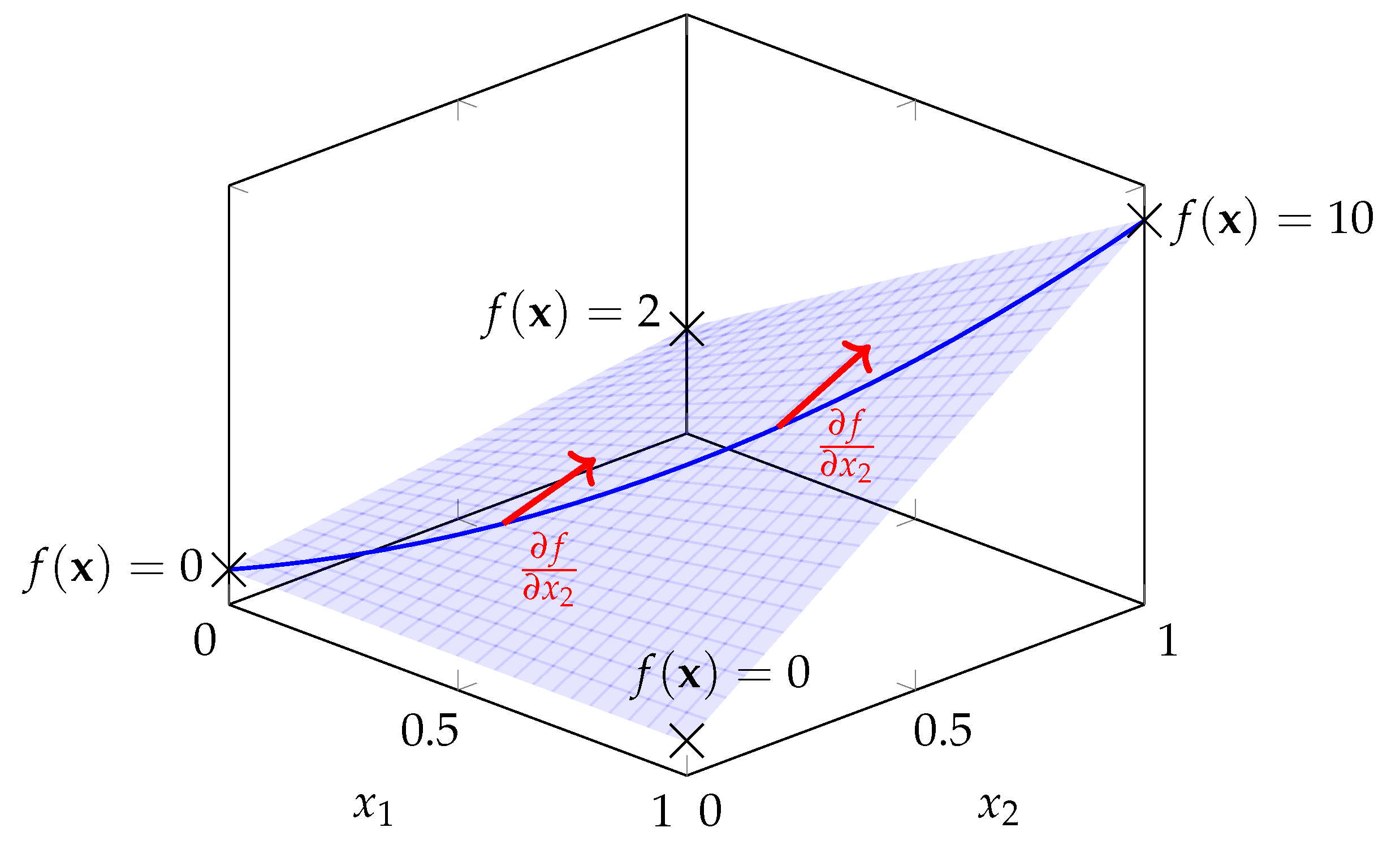
Figure 2.
The figures above visualize the expected number of coalitions of size s when running the OS algorithm for in (a) and in (b). Each color illustrates the distribution for one value as defined in (32). As in [22], we fix . One obtains that for large Q, the probability distribution converges to the true uniform distribution across coalition sizes, but for small Q, it deviates significantly from the true distribution.
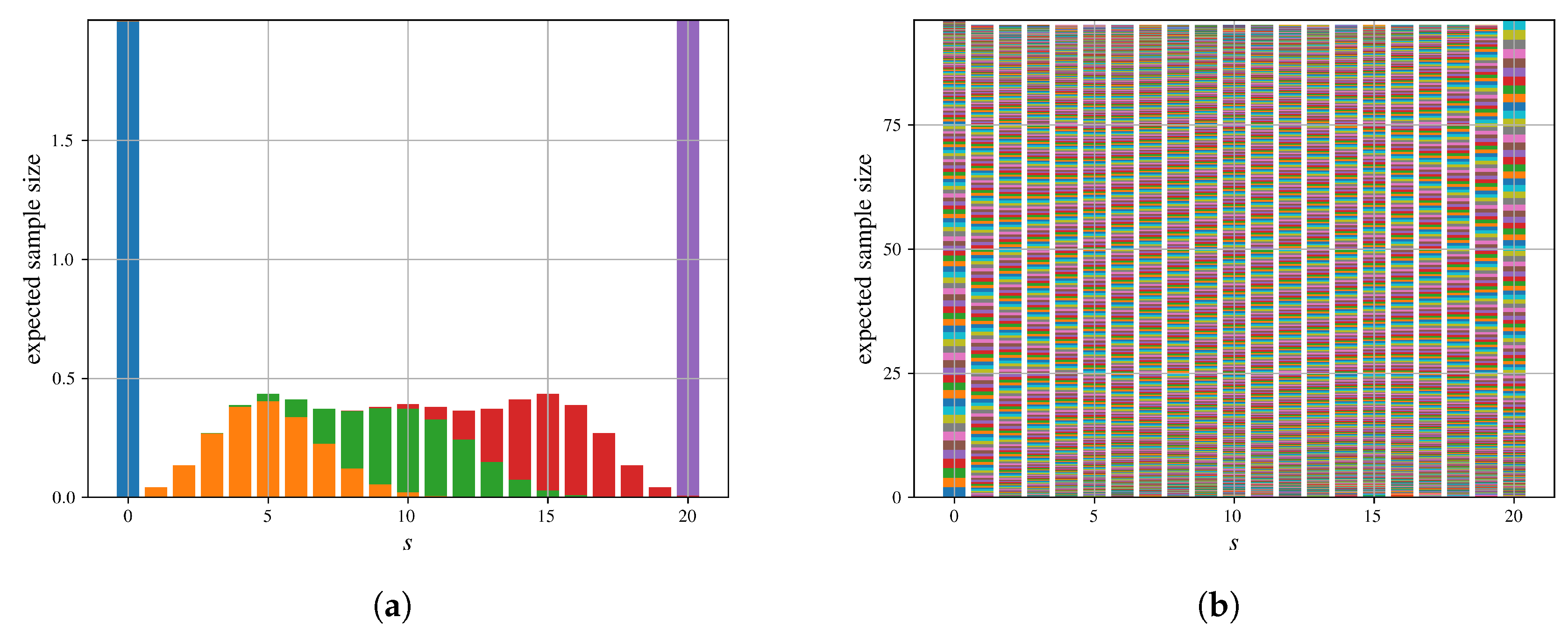
Figure 3.
Empirical bias comparison of obtained via OS, MES, and S-MES evaluated on the airport game defined by (52). The empirical biases were obtained over 5000 runs.
Figure 3.
Empirical bias comparison of obtained via OS, MES, and S-MES evaluated on the airport game defined by (52). The empirical biases were obtained over 5000 runs.
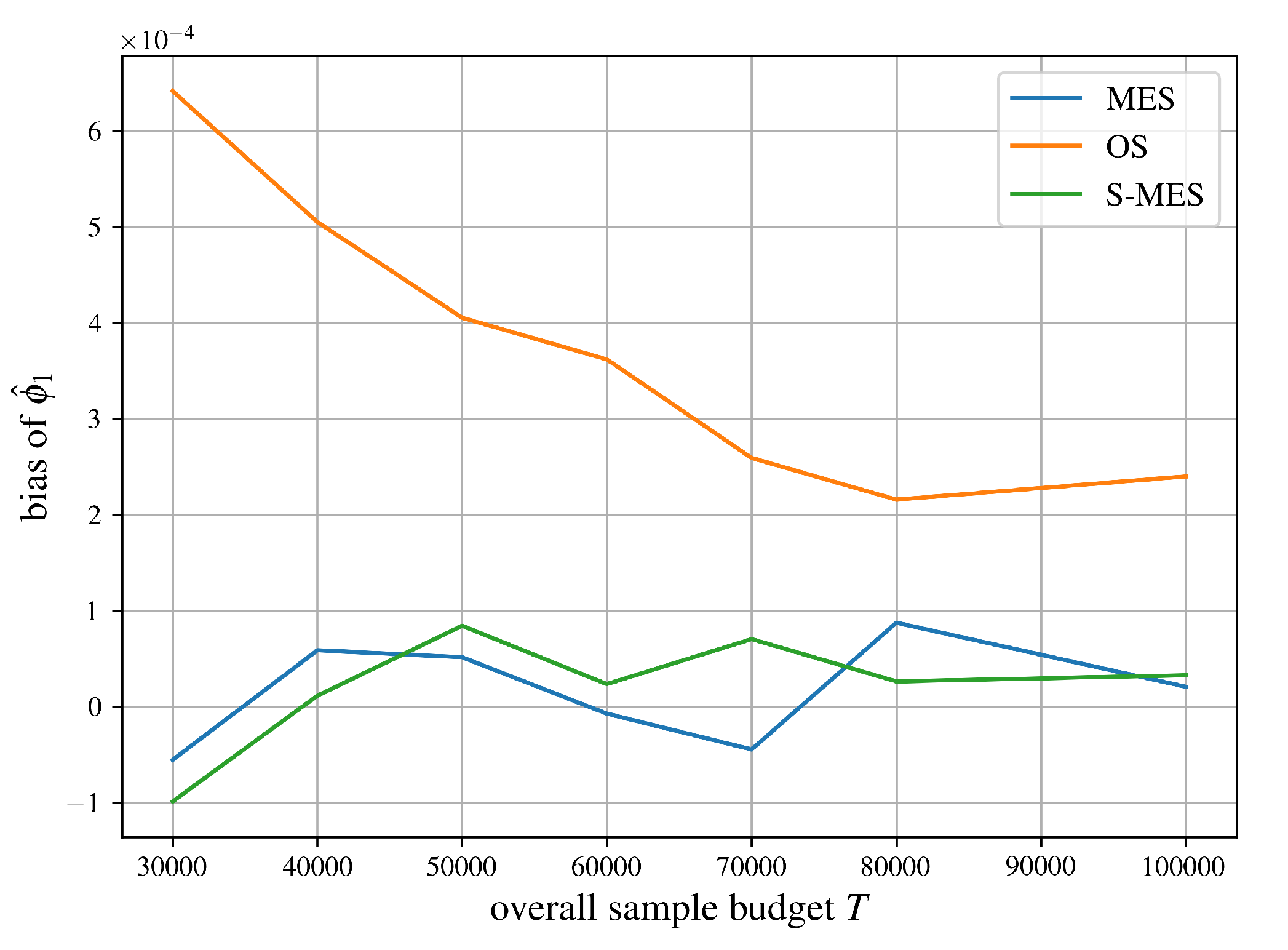
Figure 4.
Empirical variance validation of obtained via MES, MCIS and S-MCIS evaluated on the weighted voting games defined by (54). The overall sample budget is . The crosses represent the theoretical variances, while the dots denote the empirical variances. The empirical variances were obtained over 5000 runs.
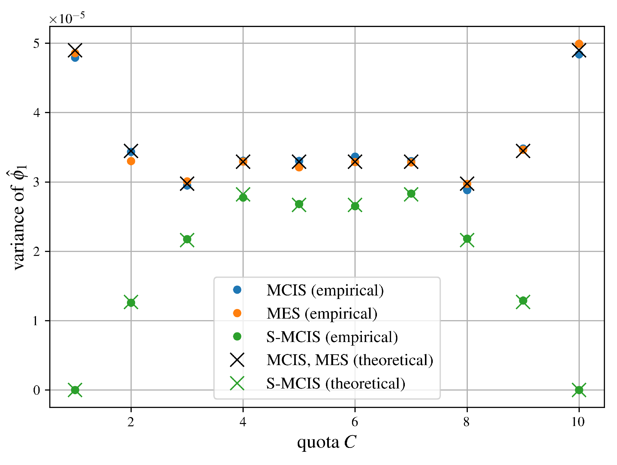
Figure 5.
Empirical mean squared error comparison of obtained via OS, MES, S-MES, MCIS, and S-MCIS evaluated on an airport game with 100 players. The mean squared errors were averaged over 250 runs.
Figure 5.
Empirical mean squared error comparison of obtained via OS, MES, S-MES, MCIS, and S-MCIS evaluated on an airport game with 100 players. The mean squared errors were averaged over 250 runs.
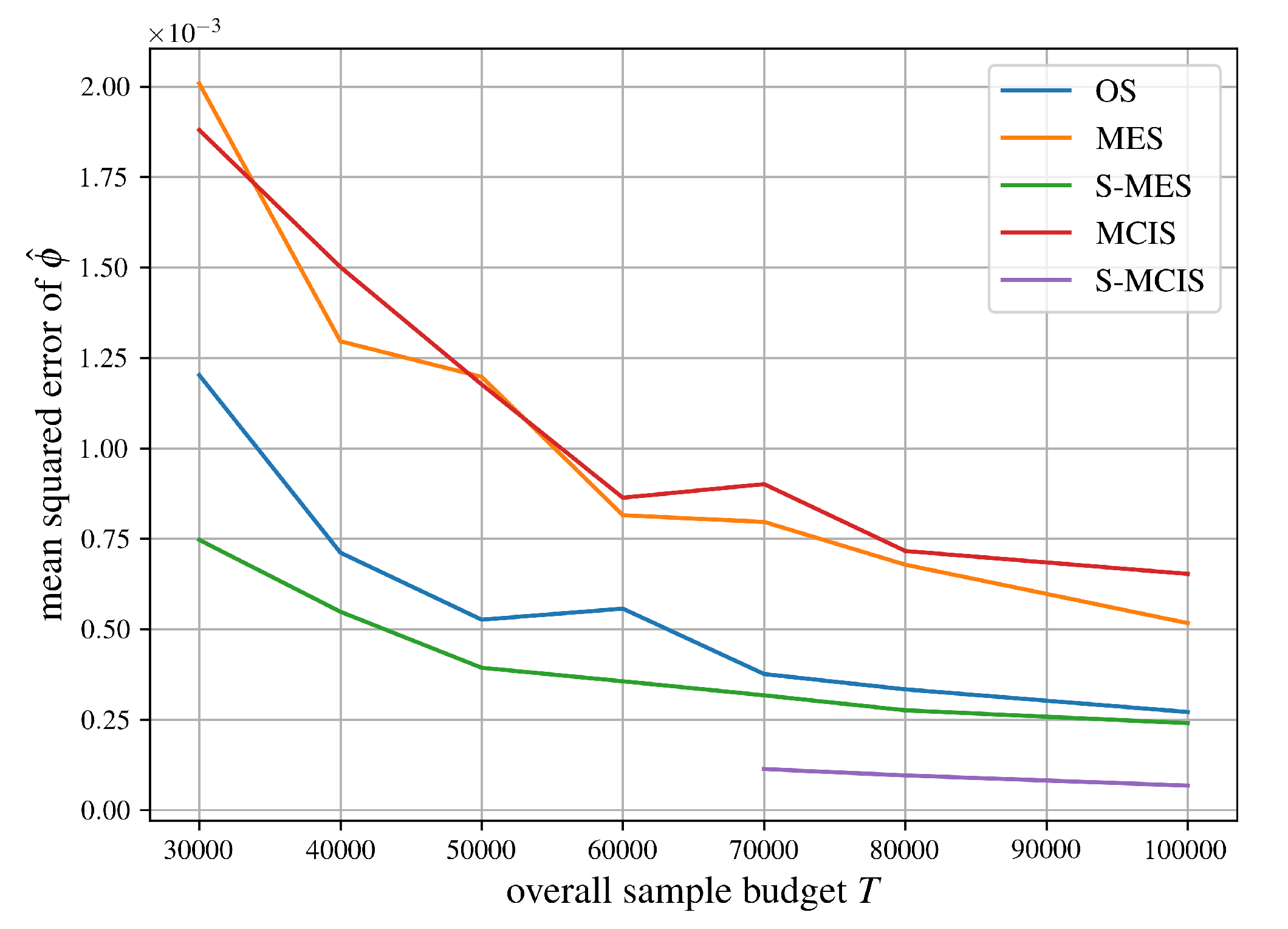
Figure 6.
Empirical mean squared error comparison of obtained via OS, MES, S-MES, MCIS, and S-MCIS evaluated on a weighted voting game with 50 players. The mean squared errors were averaged over 250 runs.
Figure 6.
Empirical mean squared error comparison of obtained via OS, MES, S-MES, MCIS, and S-MCIS evaluated on a weighted voting game with 50 players. The mean squared errors were averaged over 250 runs.
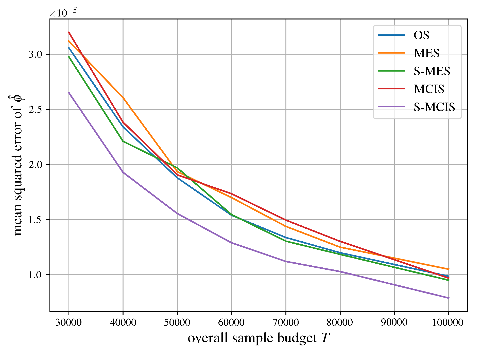
Figure 7.
Empirical mean squared error comparison of obtained via OS, MES, S-MES, MCIS, and S-MCIS evaluated on the diabetes example. The mean squared errors were averaged over 250 runs.
Figure 7.
Empirical mean squared error comparison of obtained via OS, MES, S-MES, MCIS, and S-MCIS evaluated on the diabetes example. The mean squared errors were averaged over 250 runs.
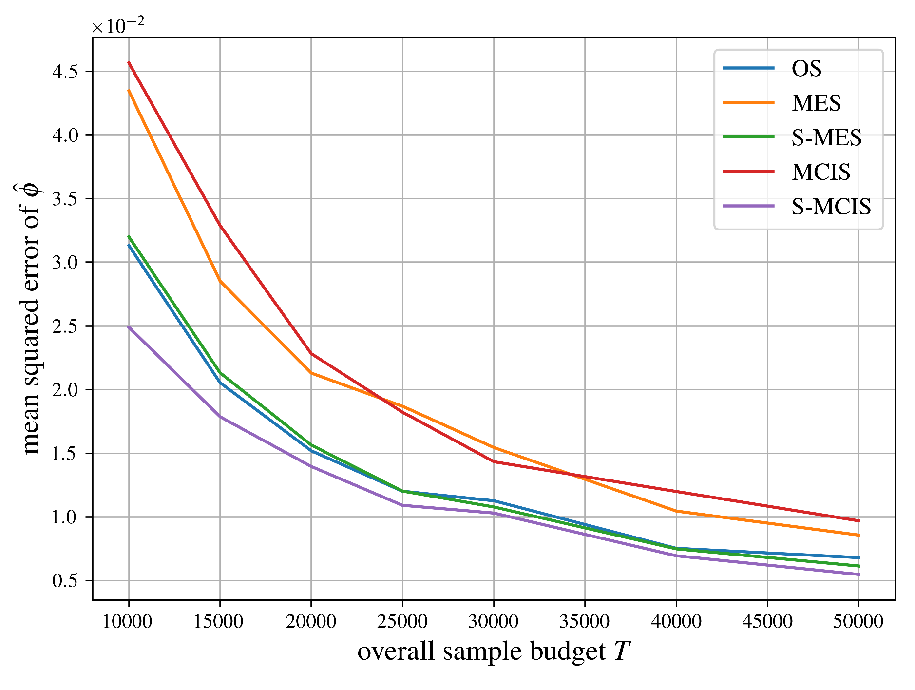
Figure 8.
Empirical mean squared error comparison of obtained via OS, MES, S-MES, MCIS, and S-MCIS evaluated on the housing example. The mean squared errors were averaged over 250 runs.
Figure 8.
Empirical mean squared error comparison of obtained via OS, MES, S-MES, MCIS, and S-MCIS evaluated on the housing example. The mean squared errors were averaged over 250 runs.
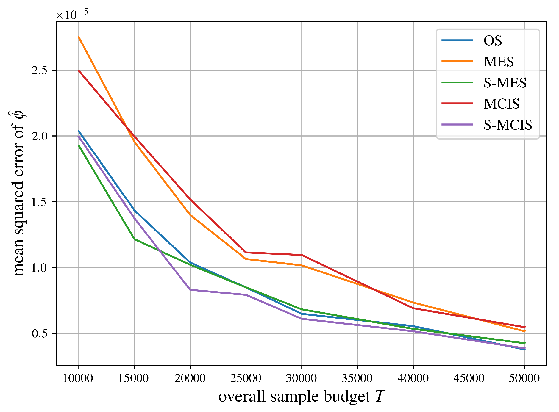
Figure 9.
Empirical mean squared error comparison of obtained via OS, MES, S-MES, MCIS, and S-MCIS evaluated on the wine example. The mean squared errors were averaged over 250 runs.
Figure 9.
Empirical mean squared error comparison of obtained via OS, MES, S-MES, MCIS, and S-MCIS evaluated on the wine example. The mean squared errors were averaged over 250 runs.
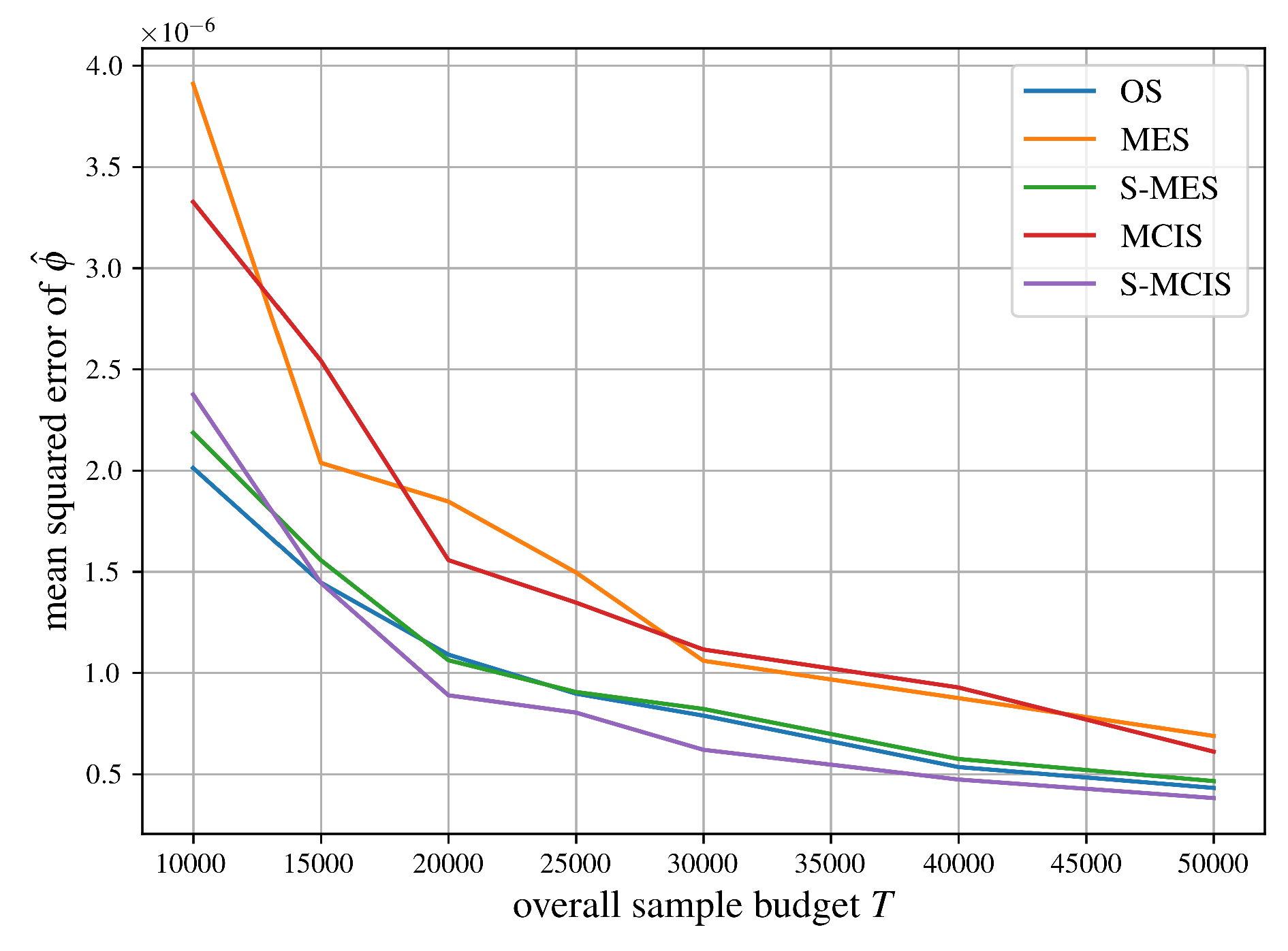
Disclaimer/Publisher’s Note: The statements, opinions and data contained in all publications are solely those of the individual author(s) and contributor(s) and not of MDPI and/or the editor(s). MDPI and/or the editor(s) disclaim responsibility for any injury to people or property resulting from any ideas, methods, instructions or products referred to in the content. |
© 2026 by the authors. Licensee MDPI, Basel, Switzerland. This article is an open access article distributed under the terms and conditions of the Creative Commons Attribution (CC BY) license (http://creativecommons.org/licenses/by/4.0/).
Copyright: This open access article is published under a Creative Commons CC BY 4.0 license, which permit the free download, distribution, and reuse, provided that the author and preprint are cited in any reuse.


