Submitted:
06 January 2026
Posted:
07 January 2026
You are already at the latest version
Abstract
The Indonesian archipelago represents one of the most tectonically complex regions on Earth, where the convergence and interaction of multiple plates drive ongoing subduction, arc-continent collision, and lithospheric accretion. To unravel the detailed structure and dynamics of this convergent margin, we develop a novel, high-resolution 3-D shear-wave velocity model of the lithosphere and upper mantle. This model is derived from a weighted joint inversion of complementary surface-wave datasets: teleseismic Rayleigh waves from 387 shallow earthquakes (MS ≥ 5.5) recorded across 31 stations, analyzed using a modified two-plane-wave tomography method, and ambient-noise correlations from two years of continuous data at 30 stations, processed with far-field approximation and image-transformation techniques. This integrated approach significantly enhances the resolution of shallow structures compared to previous body-wave tomographic models. Our model provides new insights into the four primary subduction systems. Along the Sunda-Java trench, we document a systematic along-strike transition in slab geometry: a continuous, well-defined slab in the west progressively gives way to increasingly disrupted and thickened structures eastward. This morphological evolution correlates with the subduction of progressively older oceanic lithosphere and is influenced by variations in slab age, dip, and the presence of deep slab tearing. Beneath the Banda Arc, we image an approximately 200 km-thick slab and attribute its dramatic 180° curvature to the mechanical interaction between the northward-subducting Australian plate and a distinct south-directed subduction system beneath the Seram region. In the Molucca Sea, our high-resolution tomography reveals a shallow (~50 km depth) low-velocity zone and details the complex geometry of an active double-sided subduction zone, characterized by asymmetric dips and intense seismicity, which illuminates the dynamics of ongoing arc-arc collision. Finally, beneath the Celebes Sea, a south-dipping slab is clearly resolved under North Sulawesi, while no substantial subduction signature is associated with the Sangihe Arc. Collectively, these findings provide unprecedented structural constraints on the segmentation, deformation, and interaction of subducting slabs in Indonesia. They underscore the control of lithospheric age and complex plate interactions on slab morphology and regional tectonics, offering a refined framework for understanding the geodynamic evolution of this exceptionally complex convergent boundary.
Keywords:
Indonesian archipelago
; subduction zones
; shear wave velocity
; Rayleigh wave tomography
; ambient noise tomography
1. Introduction
Located at the convergence of the Indian-Australian, Eurasian, and Philippine Sea plates, the Indonesian archipelago is one of the most tectonically complex regions on Earth. Subduction, collision, and accretion of tectonic plates occur both along and within its boundaries, contributing to the region’s unique geological characteristics. The Sundaland shelf, which forms the core of Southeast Asia, includes the Sumatra, Indochina block, southwestern Borneo, and the Java Sea, as shown in Figure 1 (Hall, 2009). As the Indian-Australian plate has subductes beneath the Eurasian plate, Borneo has undergone a significant counter-clockwise rotation (e.g. Hall, 1996; Di Leo, et al. 2012), while the southwestern part of Borneo has been involved in subduction-related accretion (Hamilton, 1979). Several fragments from the Australian plate, such as Sulawesi, have rifted off and attached to the eastern margin of Indonesia, forming seas such as the Sulu and Celebes Seas (Hall, 2009).
The most prominent subduction zone in the region is the Indian-Australian plate subducting beneath the Sumatra and Java Trenches at a rate of approximately 60 mm/yr (e.g. Muller, et al., 2008; Kundu and Gahalaut, 2011). While the Sumatra and Java Trenches appear to be continuous from northwest to southeast, the age of the subducted oceanic lithosphere varies from 40 Ma to 160 Ma between southern Sumatra and the easternmost Java (Sdrolias and Müller, 2006). Another significant difference between these trenches lies in seismicity. Earthquakes beneath Sumatra do not occur at depths greater than 300 km, whereas seismicity beneath Java is continuous at depths exceeding 670 km (Widiyantoro, et al., 2011) according to the USGS earthquake catalog.Although there is no difference in seismicity between Java Trench and Timor Trench, the collision of Australian continental lithosphere with the Banda Arc began about 5 Ma ago (e.g. Bowin, et al., 1980; Hinschberger, et al., 2005; Hall, 2009; Fichtner, et al., 2010), which has led to the uplift of the forearc region (Hamilton, 1979). The Sulawesi region, located to the northwest of Banda Arc and surrounded by Banda Sea, Molucca Sea and Celebes Sea, is one of the most geologically complex areas, hosting multiple high-density subduction zones. The Celebes Sea subducted beneath northern Sulawesi, while the Molucca Sea exhibits double-sided subduction in northeastern Sulawesi. The resulting volcanic arcs, such as the Halmahera Arc in the east and the Sangihe Arc in the west, are engaged in arc-arc collision—the only active arc-arc collision on Earth (e.g. Silver and Moore, 1978; McCaffery, 1991; Jaffe, et al., 2004). The debate continues regarding whether the double-sided subduction occurs oppositely (e.g. Djajadihardja, et al., 2004; Di Leo, et al., 2012) or face to face (e.g. McCaffrey and Silver, 1980; Hall and Wilson, 2010).
Given the region’s complexity, numerous studies have been conducted at various scales using different methods to investigate its geodynamic evolution during major plate collisions and convergence. These studies encompass geological reconstruction (e.g. Hall, 1996; 2001; 2009; Replumaz and Tapponnier, 2003; Pubellier, et al., 2004; Hinschberger, et al., 2005), seismicity (e.g. Das, 2004; Greenfield, et al., 2021), anisotropy and mantle flow (e.g. Nagao and Uyeda, 1995; Di Leo, et al., 2012; Hua, et al., 2023), and tomography (e.g. Planert, et al., 2010; Miller, et al., 2016; Zenonos, et al., 2019; Dou, et al., 2024). Hall and Spakman (2015) reviewed the P-wave velocity anomaly model UU-P07 (Amaru, 2007) which provides an overview of previous interpretations of mantle structure and tectonic history of Southeast Asia. This model offers high resolution of the deeper subduction plate, but its ability to resolve shallow structures, particularly on the lithospheric scale, remains limited.
High-resolution seismic imaging of the lithosphere is thus critical for constraining subduction slab geometry, understanding continental-arc collision relationships, and delineating complex upper mantle structures. Both surface wave tomography and ambient noise tomography provide high-resolution imaging of the lithosphere and upper mantle. These methods, when used individually or in joint inversion, have been successfully applied in various regions. For example, joint inversion for phase velocity maps in Hawaii (e.g. Le, et al., 2022), ambient noise tomography in Hainan Plume (e.g. Pan, 2024), and Surface wave tomography in Indochina block (e.g. Yang, et al., 2015) have all yielded valuable insights.
To address the resolution gap in shallow structures and obtain a more continuous image from the lithosphere into the upper mantle, this study employs a joint inversion approach. teleseismic Rayleigh waves and ambient noise data from over 30 broadband stations across Indonesia from the Incorporated Research Institutions for Seismology (IRIS) and GEOFON. For the Rayleigh wave analysis, we apply the two-plane wave approximation (Forsyth and Li, 2005) to simulate Rayleigh wave propagation, which has been used in numerous studies to obtain high-resolution results (e.g. Harmon et al., 2011; Yang, et al., 2015). For the ambient noise tomography step, we employ an image transformation technique to measure phase velocity dispersion, as introduced by Yao et al. (2005). The key advance of this work is the weighted joint inversion of these complementary phase velocity datasets to construct a robust shear-wave velocity model. This study aims to illuminate the lithospheric and upper mantle structure of this convergent boundary, providing new and independent constraints on its ongoing tectonic and geodynamic processes.
2. Data
2.1. Data Processing of Rayleigh Wave Tomography
We selected 387 shallow earthquakes from over 1600 events with magnitudes greater than Ms 5.5, and epicenter distances between 25° and 170°, occurring between 2009 and 2013. The distribution of earthquake back azimuths is as uniform as possible, as shown in Figure 2. Rayleigh waves recorded at 31 stations were processed to measure amplitudes and phases at 16 periods ranging from 20 s to 143 s. Seven stations’ data were from IRIS, and the others were from GEOFON (Germany). Figure 1 shows the station distribution, covering most of Indonesia.
We first remove the instrument response, detrend the data, and calculate the mean. Then, frequency-time analysis is applied to isolate the fundamental mode of the Rayleigh wave (Levshin et al., 1989). We measure the amplitude and phase at each period using Fourier transforms. We discard records with low signal-to-noise ratios or without a clear fundamental mode. Typically, more records are eliminated at shorter periods due to the complex topography and bathymetry in the study region. Figure 3(a) shows an example of vertical seismogram records at station CISI on Java Island from a New Hebrides earthquake (Ms 7.3, epicenter at 19.70°S, 167.95°E), filtered for periods between 20 s and 143 s. The dispersion of Rayleigh waves at different periods is clearly visible. Figure 3(b) shows similar seismograms at 50 s period from other stations in the region.
Despite careful selection of events and periods, some interference remains that affects phase velocity analysis (Forsyth et al., 2005). To account for wavefield inconsistencies across stations due to the large study region, we divide the stations into four groups for two-plane wave parameter inversion (see Figure 2 green rectangles). Earthquakes with misfits greater than 1.5 times the median are discarded, as illustrated by the Rayleigh wave raypaths at 50 s in Figure 2 (blue-gray lines).
2.2. Data Processing of Ambient Noise Tomography
Continuous vertical component seismograms recorded from 30 stations (excluding XMIS, shown as the yellow circle in Figure 1) between 2009 and 2010 were used to calculate the empirical Green’s function (EGF) and phase velocity. The LHZ component of long-period vertical records (1 Hz sampling rate) was downloaded daily. Data processing began with the removal of instrument response and spectrum whitening every 2 hours to broaden the frequency band and equilibrate the amplitude.
A key step in processing is temporal normalization, which reduces the effect of earthquakes that could obscure ambient noise (Bensen et al., 2007). We applied the running-absolute-mean normalization method, which involves averaging the absolute values of the signal within a fixed-length window. This helps mitigate earthquake interference while preserving amplitude intensity.
We then calculated ambient noise cross-correlation functions (NCFs) for 435 station pairs. The NCFs were normalized in different frequency bands (3–5 s, 5–10 s, 10–20 s, 20–40 s, 40–60 s, and 60–100 s) and stacked to form broadband NCFs, improving the signal-to-noise ratio (SNR) across different bands (Yao et al., 2006). All daily NCFs were stacked for each station pair to generate final NCFs, eliminating seasonal effects and enhancing SNR.
Previous studies (e.g. Lobkis and Weaver, 2001; Weaver and Lobkis, 2004) showed that empirical Green functions (EGFs) can be demonstrated by NCFs, that meaning
With C and is NCF and EGF between station A and station B, respectively. There is the phase shift between NCF and EGF. All of those can be used to calculate phase velocity and, in this study, we employ NCFs on it. Due to the directional inhomogeneity of the noise sources, NCFs are asymmetrical along the time axis (Bensen et al., 2007; Lin et al., 2007; Liang and Langston, 2008). We use the arithmetic mean of these NCFs as a simple and effective way to extract the dispersion curve.
3. Methods
3.1. Phase Velocity Inversion with Surface Wave
Traditional surface wave tomography assumes that surface waves propagate along great circle paths, neglecting non-planar effects caused by heterogeneities. To account for these non-planar effects, we employ the two-plane wave method (Forsyth, 1998). In this approach, the primary energy of the surface wave propagates along a slightly deviated path from the great circle, while a small amount of energy, scattered by heterogeneities, propagates along a more deviant path. The resulting surface wave is the interference of these two plane waves.
We describe the vertical displacement of the incoming Rayleigh wave at each station using six wavefield parameters: amplitude, initial phase, and propagation direction for each plane wave. This is expressed as
where A is the amplitude of each plane wave, and is the phase of each include the direction and initial phase information at kth station for ith event (Forsyth and Li, 2005). According to statistics, the vast majority of events can be represented by this way and improve resolution.
We use a grid parameterization of the study region, with 975 grid points spaced 1° by 1° and 2° by 2° at the outer rows to absorb heterogeneity. The finite-frequency sensitivity kernels are Gaussian-smoothed with a width of 150 km to account for wavefield scattering and focusing effects.
For the inversion, we first obtain a best-fitting regional 1-D velocity model across the study area based on the IASP91 model (Kennett, 1991). Then, we use this model as the initial input for 2-D phase velocity inversion at different frequencies, adjusting the phase velocity and wavefield parameters iteratively. The inversion is performed using a simulated annealing method (Press et al., 1992) followed by a linearized damped iterative least squares method (Tarantola and Valette, 1982). The least squares inversion is given by
where is the phase velocity model at iteration , is the initial model, is the change to the model, is the difference between observed and theoretical data in iteration , G is the matrix of partial derivatives with six wavefield parameters and phase velocity, is the data matrix and assumed to be diagonal and is model covariance matrix.
3.2. Phase Velocity Inversion with Ambient Noise
In this section, we employ the far-field approximation and an image transformation technique (Yao, et al., 2005) to calculate the phase velocity dispersion. First, we eliminate the NCFs which signal to noise ratio less than 3 or more complicated. We filter the records with a 0.4s width narrow band-pass filter at central periods from 5s to 100s with 4s interval. We put those filtered records together erectly by central periods as x coordinate and we obtain a time-period (t-T) image for the surface wave. Each column in the image represents an NCF after an amplitude regularization of the T in the central period (Yao, et al. 2006). Then we convert the t-T image to a phase velocity-period (c-T) image by dividing distance of the two stations. We total pick more than 239 high quality dispersion curves from the 435 noise correlation functions (see in Figure 4), but data may reduce at long periods because some distance between two stations dissatisfy greater than triple of wavelength, according to the far-field approximation (e.g. Yao, et al. 2006; Bensen, et al. 2007).
We acquire phase velocity model from ambient noise likewise using the linearized damped iterative least squares inversion (Tarantola and Valette, 1982) (eq. 3) and the same Gaussian smoothed finite-frequency sensitivity kernels to Surface wave inversion procedure. We straightforward calculated 2-D phase velocity maps within the station array from 5 to 100 s, and IASP91 model (Kennett, 1991) as a uniform initial input model, respectively.
3.3. Inversion for Shear Velocity
To obtain the shear velocity model, we use the phase velocity results from both Rayleigh wave and ambient noise tomography. We perform a joint inversion, with the Rayleigh wave phase velocity weighted more heavily due to its higher resolution. The shear velocity model is computed by linear interpolation from the 2-D phase velocity maps, using the DISPER80 code (Saito, 1988). We use the 1-D shear wave velocity model derived from the phase velocity as an initial model.
The inversion is carried out using the linearized damped iterative least squares method, with a standard deviation of 0.2 km/s for shear velocity. The initial crustal model is provided by CRUST1.0 (Laske et al., 2013) to constrain the bathymetry and crust depth.
4. Results
4.1. Resolution Tests
To validate the inversion results, we performed resolution checkboard tests with ±4% perturbations on a grid scale of 8°× 8° for both phase velocity inversions. The input model is shown in Figure 5a. For the Rayleigh wave inversion, synthetic data inherit the same event information as the real data, with each wavefield represented as the sum of two plane waves characterized by individual phase, amplitude, and propagation direction.The resolution tests at periods of 33 s, 50 s, and 77 s are presented in the panels b, d and f of Figure 5, respectively. Although minor smearing occurs at the margins, key tectonic regions such as the Sunda-Java-Banda subduction zone, Sulawesi, Celebes Sea, Molucca Sea, and Banda Sea maintain good resolution.
For the ambient noise (AN) inversion, synthetic data follow the same raypaths as the real data for each station pair. The results for periods of 33 s and 50 s are shown in Figure 5c and Figure 5e. Since there is no resolution outside the raypath coverage, we exclude those areas. However, the resolution within the station array is generally good, despite slight deformation of the rhombus pattern. The resolution for AN inversion is low at periods shorter than 13 s and longer than 77 s. In contrast, Rayleigh wave (RW) inversion provides good resolution from 25 s to 100 s due to denser raypath coverage (see Figure 2 and Figure 4).
While the resolution tests primarily reflect data coverage density, we further evaluated the confidence level of our models by calculating the twice standard error for both AN and RW data. Theses error maps are presented in Figure 5g and Figure 5h for the 33 s period at AN tomography and 55 s period at RW tomography, respectively. display the twice standard error for both data types. The upper panel shows the error at 50 s. And the error distributions are similar at other periods. Based on a 2× standard error threshold of 0.08 km/s for the RW data, a 95% confidence region was defined by a smoothed white contour. In the AN tomography results, regions with a 2× standard error below 0.12 km/s were retained, as these areas are well-supported by the raypath coverage (Figure 4b).
4.2. The 2-D Phase Velocity Results
We present the 2-D phase velocity results from RW and AN data at periods of 33 s, 40 s, 50 s, and 77 s in Figure 6. RW phase velocity perturbations are more intense and show brighter colors, indicating smaller perturbations in AN results. However, both datasets show similar patterns in most areas.
A low-velocity anomaly beneath northern Borneo and Sulawesi is visible in all maps, expanding with longer periods. High-velocity anomalies along the Sunda and Java Trenches become more pronounced at periods of 40 s and longer, aligned with the subduction direction. At 50 s and 77 s, additional high-velocity anomalies appear near the Philippine Trench, Celebes Sea and northern Sulawesi. A persistent high-velocity anomaly is observed beneath southern Borneo throughout all periods, becoming narrower at 77 s in RW results, seemingly separating the Sunda and Java Trenches from the subduction slab.
The AN velocity maps shows a high velocity perturbation in a larger area of the east, include Celebes Sea, Molucca Sea, and Banda Sea than that in RW velocity maps at the period of 33 s, 40 s and 50 s, while at the period of 77 s, the high velocity anomaly also connect with subduction zones. According to the resolution checkboard test, the RW phase velocity maps show a drag phenomenon at southwest corner and northwest corner but no effect on subduction zones.
4.3. The 3-D Shear Wave Velocity Results
The 3-D shear wave velocity structure was obtained through a weighted joint inversion of Rayleigh wave (RW) and ambient noise (AN) data. For periods between 20 s and 77 s and within the area covered by the station pair raypaths, the two datasets were combined with weights of 0.67 (RW) and 0.33 (AN). Outside the raypath coverage and for periods greater than 77 s, only RW data were used, due to lower resolution at periods greater than 77 s in AN data. The input model incorporated basin and and Moho depths from the CRUST1.0 model (Laske et al., 2013) and upper mantle shear wave velocity from the IASP91 model (Kennett & Engdahl 1991).
Figure 7 shows the shear wave velocity results obtained from the individual RW and AN inversions as well as from the joint inversion at the depth range of 40-90 km. The joint velocity maps generally align more closely with the RW results, reflecting the higher weighting assigned to RW data. The high-velocity anomalies visible in the RW maps are also reproduced in the joint maps, and the shear velocity anomalies derived from RW are generally higher than those from AN data, consistent with the observed phase velocity characteristics.
At depths of 40 km, 55 km, and 70 km, the AN results exhibit a pronounced high-velocity anomaly in the western study region that differs markedly from the RW and joint maps. At 90 km depth, the AN map shows a distinct high-velocity anomaly beneath the Banda Sea, Philippine Sea Trench, and Molucca Sea, whereas the RW map displays a negative perturbation in the same area. A low-velocity anomaly beneath northeast Borneo appears at all depths in both the RW and AN results but covers a larger area in the RW and joint maps.
Both RW and joint results reveal a low-velocity anomaly beneath Sumatra, Java, and the eastern part of Borneo. This low-velocity zone expands with increasing depth and appears to be spatially bounded by the surrounding subduction zones. At 90 km depth, the velocity perturbation reaches a minimum of -12% (3.51 km/s) beneath northwest Borneo, while the maximum velocity (4.48 km/s, +9.4%) is occurs beneath the Timor Trench.
Owing to the lower resolution of AN data at periods > 77 s, inversions for longer periods relied exclusively on RW data. Figure 8 presents horizontal slices of the shear-wave velocity model at depths of 110, 130, 150, 170, 190, and 210 km. With increasing depth, the amplitude of velocity perturbations generally decays. High-velocity anomalies associated with the Sunda, Java, Timor, and Seram trenches migrate in the direction of slab descent. The Philippine Sea subduction zone and the Molucca Sea region become more distinct at 130 km depth. At 190 km and 210 km, the high-velocity anomalies beneath the Banda Sea and Molucca Sea connect with the Philippine Sea subduction zone and extend beneath Borneo. A persistent low-velocity disturbance beneath Borneo is clearly visible at depths shallower than 170 km.
Figure 9 presents seven vertical cross-sections of the 3-D shear wave velocity model Arranged sequentially from west to east across the subduction zones within the study region. Each profile is oriented sub-perpendicular to the major subduction zones and incorporates earthquake hypocenters (magnitude MS ≥ 5.0 since 1985 from USGS) projected from a ±50 km wide corridor aligned with the profile. All seven cross-sections span from 20 km to 330 km in depth and extend laterally over 10 °, revealing contrasting shear wave velocity structures cross the Sunda Trench, Java Trench, Timor Trench, Celebes Sea and Molucca Sea regions.
The A1B1 and A2B2 profiles cross the Sunda Trench, whereas the A3B3 profile is situated near the boundary between the Sunda and Jave Trench. In the A1B1 profile, the seismicity aligns with the velocity interface separating positive and negative perturbations, which is interpreted as the boundary between the subducted and overriding slabs. The high-velocity anomalies in profiles A2B2 and A3B3 show broadly comparable geometries. In both, the anomaly extends laterally before experiencing a disruption at about 100 km depth, followed by a reappearance of a pronounced high-velocity signal between 120 and 200 km depth. This interval coincides with a marked reduction in seismicity below 100 km. These features contrast markedly with profile A1B1, where a continuous high-velocity anomaly is associated with sustained seismicity extending to about 200 km depth.
Profile A4B4 is located in the central part of the Java Trench. A thick high-velocity anomaly is observed near point A4, exhibiting a gently dipping upper interface and a poorly defined lower boundary. The anomaly extends downdip for approximately 4.5 ° along the profile, beyond which no continuous slab-like high-velocity signal is detected. Seismicity is nearly absent between depths of 200 km and 450 km, and resumes only at depths greater than 450 km. Profile A5B5, situated near the junction of the Java and Timor trenches, exhibits an anomalously thick high-velocity body (about 200 km). Its dip is steeper than that in A4B4, and it extends downdip for about 7 ° . Seismicity within this anomaly is generally low and spatially irregular, with some concentration between 4 ° and 6 ° along the profile.
Profile A6B6 traverses the Celebes Sea subduction zone and the western branch of the Molucca Sea subduction system. Within this profile, two distinct seismic trends are observed: one associated with the Celebes slab and the other with the western Molucca slab. These seismic zones converge at approximately 150 km depth and merge into a near-vertical distribution at greater depths. The dominant high-velocity anomaly aligns with the downdip direction of the Celebes Sea slab, persists from about 100 km to 250 km depth, and shows noticeable thickening below 150 km.Profile A7B7 crosses the double-sided subduction system of the Molucca Sea. A prominent low-velocity zone, approximately 50 km thick, is observed at about 50 km depth beneath this region and is accompanied by intense seismicity. This low-velocity zone thickens toward both ends of the profile. The high-velocity anomaly exhibits an asymmetric geometry: it is thicker on the eastern side and thinner with a gentler dip on the western side. The highest wave-speed within this anomaly occurs at about 200 km depth beneath the eastern subduction.
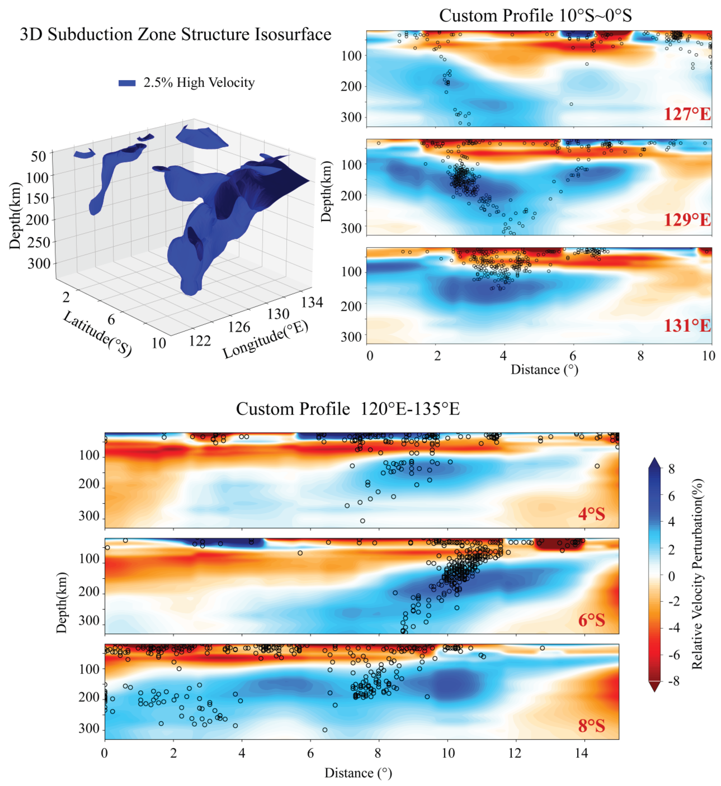
To better illustrate the structural complexity in the vicinity of the Banda Sea, we extracted the 2.5% high-velocity anomaly 3-D isosurface within in the region 0°-10° S and 120°-135° E, as shown in Figure 10. To avoid the intricate shallower structure, the iossurface is limited to the depth between 50 km and 330 km. The figure also displays three longitudinal profiles along 127°,129° and 131° E, each extending from 10° S to 0° N, as well as three latitudinal profiles along 4°, 6° and 8° S, each spaning from 120° E to 135° E. All profiles cover a depth range of 20-330 km. Following the convention of Figure 9, earthquake hypocenters are also plotted on each cross-section. A consistent feature observed in the longitudinal profiles is the presence of two subduction zones, which exhibit marked asymmetry in their high-velocity anomaly morphology and seismicity. The southern high-velocity anomaly is characterized by a stronger velocity perturbation and a higher level of seismicity. Notably, hypocenter locations show little spatial alignment with the upper interface of the high-velocity anomalies. In contrast, the latitudinal profiles indicate an east-to-west subduction trend. The high-velocity anomaly is most prominent along the 6° S profile, where seismicity also defines a coherent dipping trend. On the 4° S profile, earthquakes are more diffusely distributed, predominantly above 200 km depth. On the 8° S profile, seismicity is concentrated between two high-velocity anomalies and is largely confined to depths shallower than 200 km. As this profile transects the Timor Trench, abundant earthquakes are observed on its western side.
5. Discussion
5.1. Comparison with Previous Models
The joint surface wave (SW) and ambient noise (AN) tomographic model provides higher resolution, particularly for shallow depths (50 to 300 km), compared to earlier studies (Hall and Spakman, 2015; Legendre, et al., 2015; Zenonos, et al., 2019; Toyokauni, et al., 2022). While the imaging models of these studies, based on teleseismic P-wave or S-wave travel times, offer high resolution at greater depths, they generally provide lower resolution for lithospheric-scale structures. Previous studies have identified high-velocity anomalies across a broad region, encompassing the subduction zones of Indonesia and the Philippines. However, due to our denser raypath coverage, our velocity model reveals previously unresolved structural details.
Specifically, discrepancies are observed between our model and those of Zenonos et al. (2019) and Hall and Spakman (2015) at a depth of 100 km. Despite the indications from their model that the Bada Sea is the most significant area of low-velocity anomaly, the results of this study demonstrate that the region between Sulawesi and Borneo, as illustrated in the lateral velocity structure profiles (Figure 7 and Figure 8), exhibits the most pronounced low-velocity anomaly. Furthermore, the model demonstrates a high-velocity anomaly in the northern region of Borneo, extending from depths of 40 to 70 km, which transitions to a low-velocity anomaly at 90 km, before reverting to a high-velocity anomaly at approximately 190 km depth. This detailed structure stands in marked contrast to the broader features that were observed in earlier models.
Whilst the results obtained in this study are generally consistent with those of preceding research concerning the configuration and inclination of subduction zones, the present study provides a more comprehensive delineation of the upper interface of said subduction zones. By comparing the subduction halves and the location of seismic activity, our findings offer a clearer interpretation of the tectonic processes occurring at these depths.
5.2. The Sunda-Java Trench
The Sunda-Java Trench is the most prominent and relatively simple subduction zone in the study region,as shown in both phase velocity perturbation (Figure 6) and shear velocity perturbation maps (Figure 7 and Figure 8), particularly in the cross-section from Figure 9 (A1B1, A2B2, A3B3, A4B4 and A5B5). In the horizontal slices at 40–90 km depth, high-velocity anomalies are observed beneath the Sunda Shelf, the southern South China Sea, and northern Borneo. With increasing depth, the anomalies decrease in intensity; however, they reappear beneath northern Borneo at depths below 190 kilometres. This region has been regarded as relatively stable during the collision between the Indian and Eurasian plates(e.g. Di Leo, et al., 2012; Barber, et al., 2005; Hall, 1996). The results obtained demonstrate unequivocally the presence of a slab boundary between northern and southern Sumatra, situated in proximity to the equator (0°N), at depths of 40 to 110 km. This boundary is identified as the Wharton Fossil Ridge, distinguished by the variation in subduction vectors, ranging from 52 mm/yr to 57 mm/yr (relative plate motion vectors as determined from GPS, as referenced in Sieh and Natawidjaja, 2000).
The most prominent feature in this region is the high-velocity anomaly associated with the subduction zone. On horizontal slices, this anomaly manifests as distinct downdip propagation accompanied by progressive lateral broadening as depth increases. While the evolution of the high-velocity anomaly body is clearly observed in vertical cross-sections, they further reveal significant along-strike structural variations in slab geometry between different profiles. The five profiles on the left side of Figure 9 correspond to different segments of the subduction system. Profile A1B1 is located in close proximity to the Wharton Fossil Ridge and is distinguished by the most clearly defined subduction zone of the set. In the vicinity of point A1, the high-velocity anomaly exhibits a thickness of approximately 80 km. At a depth of 150 km, the anomaly exhibits expansion and persists continuously to depths in excess of 300 km. At depths shallower than 100 km, seismicity occurs along the upper interface of the anomaly. At greater depths, earthquakes are located within the anomaly. Profiles A2B2 and A3B3, located in the Sunda Trench and the boundary between the Sunda and Java trenches respectively, exhibit a similar geometry of high-velocity anomalies, characterised by an interruption at a depth of approximately 100 km, followed by the reappearance of a block-shaped anomaly at greater depths where seismicity is notably diminished. One potential explanation for this phenomenon is that the older, rigid slabs beneath Sunda and Java have undergone vertical tearing at depths of approximately 100 km. This phenomenon enables the ascent of hot asthenospheric material through the slab window that is formed. The upwelling hot mantle exerts a significant erosive force on the upper portion of the originally cold slab, concurrently inducing thermal heating. Consequently, the temperature difference between the slab and the surrounding mantle diminishes in the region above 100 km depth, causing parts of the slab to lose the pronounced high-velocity anomaly typical of cold subducting plates. The main body of the slab continues to descend beneath the tear window. It is evident that, upon evading the superficial thermal perturbation, this segment maintains its low-temperature properties. Consequently, a distinct high-temperature velocity anomaly manifests itself below 100 km. Profile A4B4 is located in the central part of the Java Trench and exhibits a geometry that is distinct from the geometry of the previous three subduction-zone profiles. In the vicinity of point A4, a substantial high-velocity anomaly is identified, characterised by a gently dipping upper interface and a poorly defined lower boundary. The anomaly extends downwards for approximately 4.5° along the profile, beyond which no clear slab-like high-velocity signal is detected. However, seismicity patterns indicate that earthquakes are almost non-existent between 200 and 450 km depth, and only resume at depths greater than 450 km. This may imply that the subducted slab is fragmented at depths beyond the resolution of the model, a feature that could be attributed to the older age of the subducting lithosphere beneath A4B4 compared to the three preceding trench segments. Profile A5B5, interpreted as the transition between subduction of oceanic and continental lithosphere, exhibits an unusually thick slab of approximately 200 km and a steeper dip compared to profile A4B4. Its geometry differs further from that of the four previously described subduction segments. Along the profile, the slab extends downwards for approximately 7°. Seismicity within the high-velocity anomaly is generally low and spatially irregular, though earthquakes show some concentration between 4° and 6° along the profile.
Overall, from A1B1 to A5B5, the geometry of the high-velocity anomalies exhibits a systematic transition: continuous and intact slabs in the west progressively give way to increasingly complex structures toward the east, characterised by disruption, thickening, and deep seismic gaps. This spatial evolution is indicative of the subduction transition from juvenile oceanic lithosphere to more mature continental lithosphere of the Indo-Australian plate. The observed morphological disparities are predominantly influenced by dynamic processes, including slab age, dip angle, and deep slab tearing.
5.3. The Banda Arc
The Australian plate is moving northward at a high rate of approximately 70 mm/yr (Bock, et al., 2003). In the vicinity of Sumba Island (approximately 120° E), between the easternmost end of the Java Trench and the westernmost end of the Timor Trench, pronounced tectonic deformation has developed, demarcating the arc-continent collision boundary between the Australian plate and the Banda Arc. As demonstrated in Figure 7 and Figure 8, this deformation commences at a depth of approximately 55 km, reflecting flexural deformation of the oceanic lithosphere caused by ongoing subduction as it interacts with the continental lithosphere of Australia.
As demonstrated in Figure 8, the horizontal slices of the lithosphere and upper mantle, reveal the extent of the high-velocity Banda slab. This slab extends from Sumba in the west to Aru in the east, and continues northward toward Seram. The high-velocity anomaly layer beneath the Banda Arc is approximately 200 km thick, a result consistent with the thickness of the Precambrian Australian lithosphere inferred from the global P-wave tomography model BS2000 by Bijwaard & Spakman (2000) and from full-waveform tomography by Fichtner et al. (2010).
In order to establish the subduction setting of the Banda Arc, vertical cross-sections were constructed at 2° intervals in both the longitudinal and latitudinal directions (see Figure 10).When integrated with seismicity distributions, these sections indicate that the pronounced curvature (approximately 180°) of the Banda Arc is likely the result of the interaction of two distinct subduction systems.The initial system is indicative of the northward subduction of the Australian plate along the Timor Trench, which appears to terminate in proximity to the Tarera–Aiduna Fault Zone. This segment exhibits intense seismicity, with the highest concentration of earthquakes occurring between 100 and 200 km depth, coinciding with the core of the local high-wave-speed anomaly.The second system is characterised by south-directed subduction beneath Seram, a process that is likely associated with the underthrusting of the Bird’s Head Block. In contrast, this zone exhibits significantly reduced seismicity and is distinguished by a comparatively lower-amplitude high-wave-speed anomaly. Among the three longitudinal profiles, the 127°E profile, located at the western boundary of the Seram Trench, exhibits an irregular high-velocity anomaly. This anomaly is connected with Timor at approximately 200 km, while the 129°E profile is connected at 100 km. The high-velocity anomaly body begins to converge and narrow around 250 km. At the 131°E profile, seismic activity occurs at depths not exceeding 150 km, with the high-velocity anomaly bodies fully coalescing into a shape resembling a “table knife”. It is evident from the three latitudinal profiles that the subduction angle demonstrates a gradual decline in steepness, moving from the western to the eastern boundary of the Timor Trench. The maximum velocity of the high-velocity anomaly is observed to occur in the vicinity of 130°E. The seismic activity distribution exhibited in the 6° S profile manifests distinct subduction tectonic characteristics. During its northward subduction, the Timor Trench subduction zone gradually turns northwestward in the Aru region. This turn also provides the conditions for the Banda Arc to form a 180° loop.
5.4. The Molucca Sea Arc-Arc Collision
Profiles A6B6 and A7B7 in Figure 9 traverse the double subduction of the Molucca Sea and the Celebes subduction zone, respectively. The Molucca Sea subducts eastward beneath the Halmahera Arc and westward beneath the Sangihe Arc. Although no clear trench or active arc-arc collision is presently observed (e.g., Hall, 1987; McCaffrey et al., 1980; Silver & Moore, 1978), the convergence and near-vertical merging of two distinct seismic zones below 150 km depth in A6B6 suggest that the subducting Celebes slab and the western Molucca slab collide at this level. The dominance of the high-velocity anomaly aligned with the Celebes slab indicates that its structural imprint overpowers that of the western Molucca slab in the imaged volume, which could be due to a combination of greater slab thickness, faster subduction rate, or more intact slab integrity. Profile A7B7 (Figure 10) shows that the Molucca Sea region is underlain by an about 50 km thick low-velocity zone at approximately 50 km depth, which is accompanied by intense seismicity and thickens toward both ends of the profile. Two back-to-back subduction zones centered near 4° display different dip angles, with the highest velocity anomaly occurring at about 200 km depth beneath the eastern subduction. The UU-P07 P-wave model (Amaru, 2007), as reviewed by Hall & Spakman (2015), does not show a similarly thick low-velocity zone above the subduction system. Our surface wave tomography provides higher lithospheric resolution and reveals this feature in greater detail. This low-velocity anomaly may result from the dynamics of the arc-arc collision zone, where subduction collision interaction induces mantle resistance and slab deformation. The process is expected to continue for several million years before the collision zone likely vanishes beneath the Halmahera Arc (Hall, 2002).
6. Conclusions
We have presented a new 3-D shear-wave velocity model of the Indonesian subduction system derived from a joint inversion of Rayleigh wave and ambient noise phase velocity data. This approach significantly enhances the resolution of lithospheric and uppermost mantle structures compared to previous P-and S-wave global tomographic models, particularly particularly in resolving the shape and characteristics of subducting slabs.
The model reveals systematic along-strike variations in slab morphology from west to east. Beneath the Sunda-Java trench, the slab transitions from a continuous, coherent high-velocity anomaly in the west to increasingly disrupted and thickened structures eastward, with evidence of slab tearing near 100 km depth, a deep seismic gap beneath central Java, and pronounced slab thickening near the Timor-Banda junction. These changes reflect the progressive involvement of older continental lithosphere of the Indo-Australian plate and are governed by variations in slab age, dip, and deep tearing. In the Banda Arc region, the pronounced about 180° curvature is interpreted as the result of interaction between two subduction systems: northward subduction of the Australian plate and south-directed underthrusting beneath Seram.Within the Molucca Sea collision zone, our high-resolution tomography reveals a shallow (about 50 km depth), seismically active low-velocity zone that is not resolved in previous global models. This feature likely reflects ongoing arc-arc collision dynamics, illustrating how double-sided subduction and slab interaction are accommodated in the upper mantle.
Overall, this study provides an improved structural framework for understanding one of Earth’s most tectonically complex convergent margins. The integration of multi-scale surface wave data not only clarifies the geometry and segmentation of subducting slabs but also highlights the interplay between subduction dynamics, slab tearing, and plate-scale bending. These results offer a foundation for future geodynamic modelling aimed at quantifying the temporal evolution of subduction and collision processes in the region.
References
- Amaru, M.L. Global travel time tomography with 3-D reference models. PhD thesis, Utrecht University, 2007. [Google Scholar]
- Sumatra: Geology, Resources and Tectonic Evolution. In Geol. Soc. London Mem.; Barber, A.J., Crow, M.J., Milsom, J.S., Eds.; 2005; Volume 31. [Google Scholar]
- Bensen, G.D.; Ritzwoller, M.H.; Barmin, M.; Levshin, A.L.; Lin, F.C.; Moschetti, M.P.; Shapiro, N.M.; Yang, Y. Processing seismic ambient noise data to obtain reliable broadband surface wave dispersion measurements. Geophys. J. Int. 2007, 169(3), 1239–1260. [Google Scholar] [CrossRef]
- Bijwaard, H.; Spakman, W. Nonlinear global P-wave tomography by iterated linearized inversion. Geophys. J. Int. 2000, 141, 71–82. [Google Scholar] [CrossRef]
- Bird, P. An updated digital model of plate boundaries. Geochem. Geophys. Geosyst 2003, 4(3). [Google Scholar] [CrossRef]
- Bock, Y.; Prawirodirdjo, L.M.; Genrich, J.F.; Stevens, C.; McCaffrey, R.; Subarya, C.; Puntodewo, S.S.O.; Calais, E. Crustal motion in Indonesia from Global Positioning System measurements. J. Geophys. Res. 2003, 108, B8. [Google Scholar] [CrossRef]
- Bowin, C.; Purdy, G.M.; Johnston, C.; Shor, G.; Lawver, L.; Hartono, H.M.S.; Jezek, P. Arc–continent collision in the Banda Sea region. AAPG Bull. 1980, 64, 868–915. [Google Scholar]
- Das, S. Seismicity gaps and the shape of the seismic zone in the Banda Sea region from relocated hypocenters. J. Geophys. Res. 2004, 109. [Google Scholar] [CrossRef]
- Di Leo, J.F.; Wookey, J.; Hammond, J.O.S.; Kendall, J.-M.; Kaneshima, S.; Inoue, H.; Yamashina, T.; Harjadi, P. Mantle flow in regions of complex tectonics: Insights from Indonesia. Geochem. Geophys. Geosyst 2012, 13, Q12008. [Google Scholar] [CrossRef]
- Djajadihardja, Y.S.; Taira, A.; Tokuyama, H.; Aoike, K.; Reichert, C.; Block, M.; Schluter, H.U.; Neben, S. Evolution of an accretionary complex along the north arm of the island of Sulawesi, Indonesia. Isl. Arc 2004, 13, 1–17. [Google Scholar] [CrossRef]
- Dou, H.; Xu, Y.; Lebedev, S.; de Melo, B. C.; van der Hilst, R. D.; Wang, B.; Wang, W. The upper mantle beneath Asia from seismic tomography, with inferences for the mechanisms of tectonics, seismicity, and magmatism. Earth-Science Reviews 2024, 104841. [Google Scholar] [CrossRef]
- Fichtner, A.; De Wit, M.J.; Van Bergen, M. Subduction of continental lithosphere in the Banda Sea region: Combining evidence from full waveform tomography and isotope ratios. Earth Planet. Sci. Lett. 2010, 405–412. [Google Scholar] [CrossRef]
- Forsyth, D.W.; Webb, S.C.; Dorman, L.M.; Shen, Y. Phase velocities of Rayleigh waves in the MELT experiment on the East Pacific Rise. Science 1998, 280, 1235–1238. [Google Scholar] [CrossRef] [PubMed]
- Forsyth, D.W.; Li, A. Array analysis of two-dimensional variations in surface wave phase velocity and azimuthal anisotropy in the presence of multipathing interference. In Seismic Earth: Array Analysis of Broadband Seismograms; AGU Geophysical Monograph Series: Washington, DC, 2005; pp. 81–98. [Google Scholar]
- Greenfield, T.; Gilligan, A.; Pilia, S.; Cornwell, D. G.; Tongkul, F.; Widiyantoro, S.; Rawlinson, N. Post-subduction tectonics of Sabah, northern Borneo, inferred from surface wave tomography. Geophysical Research Letters 2022, 49, e2021GL096117. [Google Scholar] [CrossRef]
- Hall, R. Plate boundary evolution in the Halmahera region, Indonesia. Tectonophysics 1987, 144, 337–352. [Google Scholar] [CrossRef]
- Hall, R.; Blundell, D.J. Tectonic evolution of SE Asia: Introduction. Geol. Soc. Lond. Spec. Publ. 1996, 106(1). [Google Scholar] [CrossRef]
- Hall, R.; Wilson, M.E. Neogene sutures in eastern Indonesia. J. Asian Earth Sci. 2000, 18(6), 781–808. [Google Scholar] [CrossRef]
- Hall, R. Cenozoic geological and plate tectonic evolution of SE Asia and the SW Pacific: Computer-based reconstructions, models, and animations. J. Asian Earth Sci. 2001, 20, 351–431. [Google Scholar] [CrossRef]
- Hall, R. Cenozoic geological and plate tectonic evolution of SE Asia and the SW Pacific: computer-based reconstructions, model and animations. J. Asian Earth Sci. 2002, 20, 353–431. [Google Scholar] [CrossRef]
- Hall, R. The Eurasian SE Asian margin as a modern example of an accretionary orogen. Geol. Soc. Lond. Spec. Publ. 2009, 318, 351–372. [Google Scholar] [CrossRef]
- Hall, R.; Spakman, W. Mantle structure and tectonic history of SE Asia. Tectonophysics 2015, 658, 14–45. [Google Scholar] [CrossRef]
- Hamilton, W. Tectonics of the Indonesian region. U. S. Geological Survey Professional Paper 1979, 1078, 345 pp. [Google Scholar]
- Harmon, N.; Forsyth, D.W.; Weeraratne, D.S.; Yang, Y.; Webb, S.C. Mantle heterogeneity and off-axis volcanism on young Pacific lithosphere. Earth Planet. Sci. Lett. 2011, 311, 306–315. [Google Scholar] [CrossRef]
- Hinschberger, F.; Malod, J.; Rehault, J.; Villeneuve, M.; Royer, J.; Burhanuddin, S. Late Cenozoic geodynamic evolution of eastern Indonesia. Tectonophysics 2005, 91–118. [Google Scholar] [CrossRef]
- Hua, Y.; Zhao, D.; Xu, Y.-G. P and S wave anisotropic tomography of the Banda subduction zone. Geophysical Research Letters 2023, 50, e2023GL105611. [Google Scholar] [CrossRef]
- Jaffe, L. A.; Hilton, D. R.; Fischer, T. P.; Hartono, U. Tracing magma sources in an arc-arc collision zone: Helium and carbon isotope and relative abundance systematics of the Sangihe Arc, Indonesia. Geochem. Geophys. Geosyst 2004, 5, Q04J10. [Google Scholar] [CrossRef]
- Kennett, B.L.N.; Engdahl, E.R. Travel times for global earthquake location and phase association. Geophys. J. Int. 1991, 105, 429–465. [Google Scholar] [CrossRef]
- Kundu, B.; Gahalaut, V.K. Slab detachment of subducted Indo-Australian plate beneath Sunda arc, Indonesia. Journal of Earth System Science 2011, 120(2), 193–204. [Google Scholar] [CrossRef]
- Laske, G.; Masters, G.; Ma, Z.; Pasyanos, M. Update on CRUST1.0—a 1-degree Global Model of Earth’s crust. Geophys. Res. Abstr. 2013, 15. [Google Scholar]
- Le, B.M.; Yang, T.; Morgan, J.P. Seismic Constraints on Crustal and Uppermost Mantle Structure Beneath the Hawaiian Swell: Implications for Plume-Lithosphere Interactions. J. Geophys. Res. Solid Earth 2022, 127, e2021JB023822. [Google Scholar] [CrossRef]
- Legendre, C.P.; Zhao, L.; Chen, Q.-F. Upper-mantle shear-wave structure under East and Southeast Asia from Automated Multimode Inversion of waveforms. Geophys. J. Int. 2015, 203, 707–719. [Google Scholar] [CrossRef]
- Levshin, A.L.; Yanocskaya, T.B.; Lander, A.V.; Bukchin, B.G.; Barmin, M.P.; Ratnikova, L.I.; Its, E.N. Seismic surface waves in a laterally inhomogeneous Earth; Keilis-Borok, V.I., Ed.; Kluwer Academic Publishers: Dordrecht, 1989; pp. 153–163. [Google Scholar]
- Liang, C.; Langston, C.A. Ambient seismic noise tomography and structure of eastern North America. J. Geophys. Res. 2008, 113, B03309. [Google Scholar] [CrossRef]
- Lin, F.C.; Ritzwoller, M.H.; Townend, J.; Bannister, S.; Savage, M.K. Ambient noise Rayleigh wave tomography of New Zealand. Geophysical Journal International 2007, 170(2), 649–666. [Google Scholar] [CrossRef]
- Lobkis, O.I.; Weaver, R.L. On the emergence of the Green’s function in the correlations of a diffusive field. J. acoust. Soc. Am. 2001, 110, 3011–3017. [Google Scholar] [CrossRef]
- McCaffery, R.; Silver, E.A. Crustal Structure of the Molucca Sea Collision Zone, Indonesia. The Tectonic and Geologic Evolution of Southeast Asian Seas and Islands—Geophysical Monograph 1980, 23. [Google Scholar]
- McCaffrey, R. Earthquakes and ophiolite emplacement in the Molucca Sea Collision Zone, Indonesia. Tectonics 1991, 10(2), 433–453. [Google Scholar] [CrossRef]
- Miller, M.S.; O’Driscoll, L.J.; Roosmawati, N.; Harris, C.W.; Porritt, R.W.; West, A.J. Banda Arc Experiment—Transitions in the Banda Arc-Australian Continental Collision. Seismological Research Letters 2016, 87(6). [Google Scholar] [CrossRef]
- Muller, C.; Barckhausen, U.; Ehrhardt, A.; Engels, M.; Gaedicke, C.; Keppler, H.; Flueh, E.R.; Djajadihardja, Y.S.; Soemantri, D.; Seeber, L. From Subduction to Collision: The Sunda-Banda Arc Transition. Eos, Transactions American Geophysical Union 2008, 89(6), 49–50. [Google Scholar] [CrossRef]
- Nagao, T.; Uyeda, S. Heat-flow distribution in Southeast Asia with consideration of volcanic heat. Tectonophysics 1995, 251, 153–159. [Google Scholar] [CrossRef]
- Pan, M.; Yang, T.; Le, B.M.; Dai, Y.; Xiao, H. The Magmatic Patterns Formed by the Interaction of the Hainan Mantle Plume and Lei–Qiong Crust Revealed through Seismic Ambient Noise Imaging. Geosciences 2024, 14, 63. [Google Scholar] [CrossRef]
- Planert, L.; Kopp, H.; Lueschen, E.; Mueller, C.; Flueh, E. R.; Shulgin, A.; Djajadihardja, Y.S.; Krabbenhoeft, A. Lower plate structure and upper plate deformational segmentation at the Sunda-Banda arc transition, Indonesia. Journal of Geophysical Research 2010, 115, B8. [Google Scholar] [CrossRef]
- Press, W.H.; Teukolsky, S.A.; Vetterling, W.T.; Flannery, B.P. Numerical Recipes in FORTAN: The Art of Scientific Computing, 2nd edn; Cambridge Univ. Press, 1992; p. 963. [Google Scholar]
- Pubellier, M.; Monnier, C.; Maury, R.C.; Tamayo, R.A. Plate kinematics, origin and tectonic emplacement of supra-subduction ophiolites in SE Asia. Tectonophysics 2004, 9–36. [Google Scholar] [CrossRef]
- Replumaz, A.; Tapponnier, P. Reconstruction of the deformed collision zone Between India and Asia by backward motion of lithospheric blocks. Journal of Geophysical Research 2003, 108(B6), 2285. [Google Scholar] [CrossRef]
- Saito, M. DISPER80: a subroutine package for the calculation of seismic normal mode solutions. In Seismological Algorithms: Computational Methods and Computer Programs; Doornbos, D.J., Ed.; Elsevier, 1988; pp. 293–319. [Google Scholar]
- Sdrolias, M.; Müller, R.D. Controls on back-arc basin formation. Geochem. Geophys. Geosyst 2006, 7, Q04016. [Google Scholar] [CrossRef]
- Sieh, K.; Natawidjaja, D. H. Neotectonics of the Sumatran fault, Indonesia. Journal of Geophysical Research 2000, 28295–28326. [Google Scholar] [CrossRef]
- Silver, E.A.; Moore, J.C. The Molucca Sea Collision Zone, Indonesia. Journal of Geophysical Research 1978, 1681–1691. [Google Scholar] [CrossRef]
- Tarantola, A.; Valette, B. Generalized nonlinear inverse problems solved using the least squares criterion. Rev. geophys. Space Phys. 1982, 20(2), 219–232. [Google Scholar] [CrossRef]
- Toyokuni, G.; Zhao, D.; Kurata, K. Whole-mantle tomography of Southeast Asia: New insight into plumes and slabs. Journal of Geophysical Research: Solid Earth 2022, 127, e2022JB024298. [Google Scholar] [CrossRef]
- Weaver, R.L.; Lobkis, O.I. Diffuse fields in open systems and the emergence of the Green’s function. J. acoust. Soc. Am. 2004, 116, 2731–2734. [Google Scholar] [CrossRef]
- Widiyantoro, S.; Pesicek, J.D.; Thurber, C.H. Subducting slab structure below the eastern Sunda arc inferred from non-linear seismic tomographic imaging; Geological Society, London, Special Publications, 2011; Volume v.355, pp. 139–155. [Google Scholar] [CrossRef]
- Yang, T.; Liu, F.; Harmon, N.; Phon Le, K.; Gu, S.; Xue, M. Lithospheric structure beneath Indochina block from Rayleigh wave phase velocity tomography. Geophys. J. Int. 2015, 200, 1582–1595. [Google Scholar] [CrossRef]
- Yao, H.; Xu, G.; Zhu, L.; Xiao, X. Mantle structure from inter-station Rayleigh wave dispersion and its tectonic implication in western China and neighboring regions. Physics of the Earth and Planetary Interiors 2005, 148(1), 39–54. [Google Scholar] [CrossRef]
- Yao, H.; van der Hilst, R.D.; de Hoop, M.V. Surface-wave array tomography in SE Tibet from ambient seismic noise and two-station analysis: I - Phase velocity maps. Geophysical Journal International 2006, 732–744. [Google Scholar] [CrossRef]
- Zenonos, A.; De Siena, L.; Widiyantoro, S.; et al. P and S wave travel time tomography of the SE Asia-Australia collision zone. Physics of the Earth and Planetary Interiors 2019, 293, 106267. [Google Scholar] [CrossRef]
Figure 1.
Map of Indonesia and adjacent regions with tectonic plate boundaries, subduction zones, major faults (redraw after Bird, 2003; Djajadihardja, et al. 2004; Hall & Wilson, 2000), and seismic stations (red circles and the yellow one) used in this study. Bu: Buru; BH: Bird’s Head; SFZ: Sorong Fault zone; TAFZ: Tarera Aiduna Fault zone; MS: Molucca Sea; WD: Weber Deep according to Spakman & Hall (2010) and Djajadihardja, et al. (2004). The location of extinct Wharton Fossil Ridge came from Sdrolias and Müller (2006).
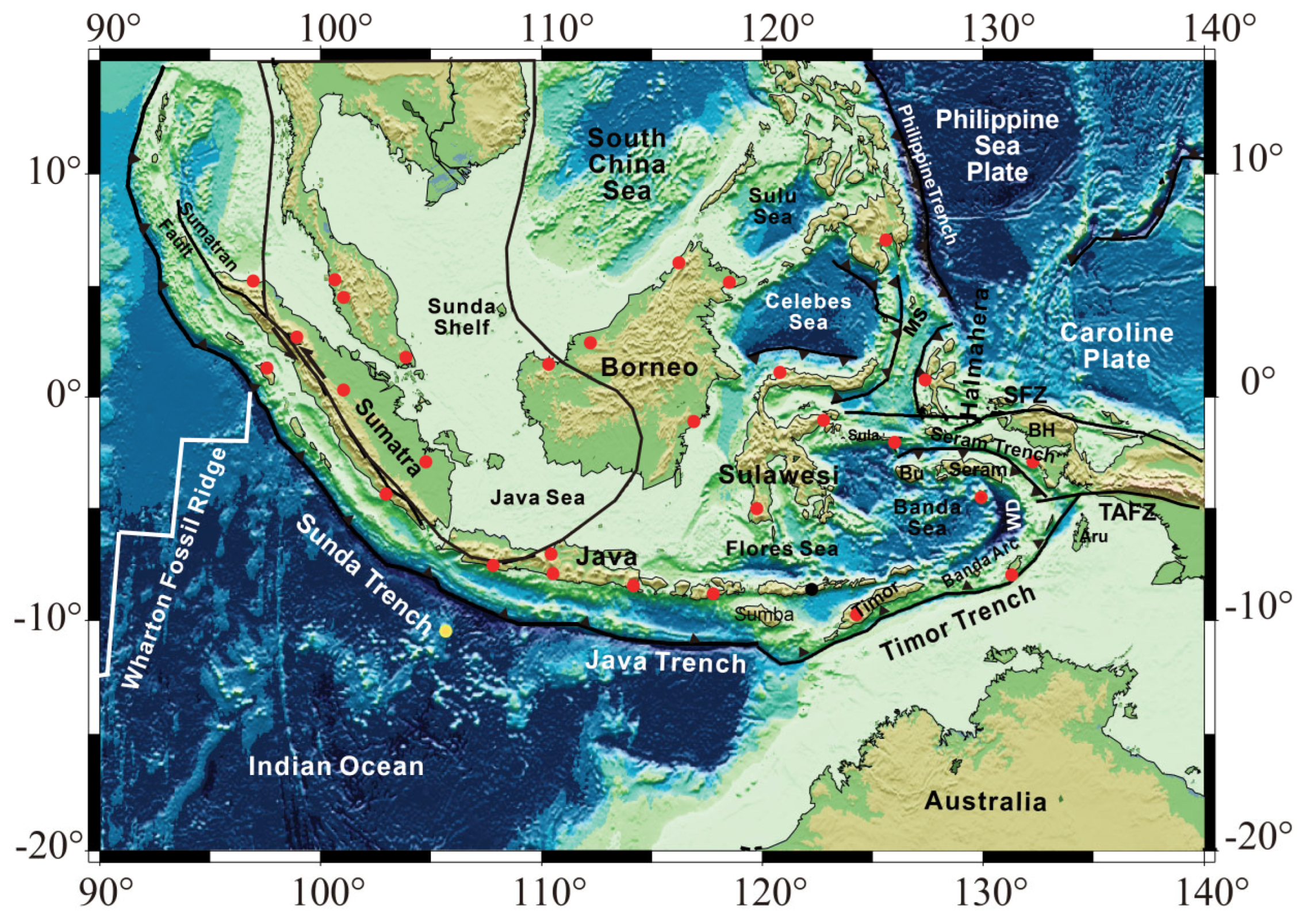
Figure 2.
The study region is parameterized by grid nodes shown as open circles. Red squares mark seismic stations. The blue gray lines are great circle raypaths of all Rayleigh waves at the period of 50s. Stations in four green rectangles were taken as a group in the inversion to inverse the initial two-plane wave parameters. Inset map shows the distribution of the earthquakes used as Rayleigh wave sources.
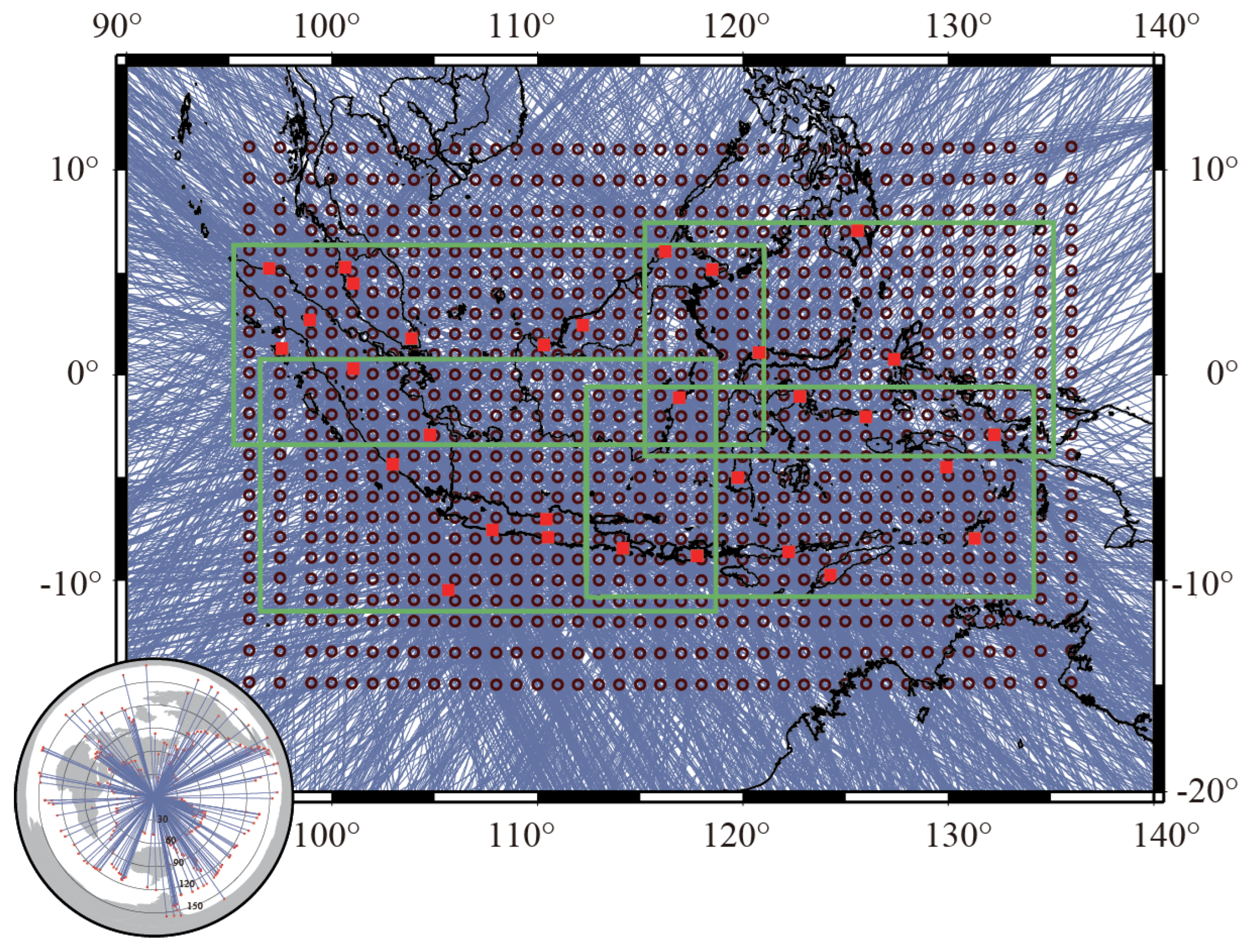
Figure 3.
Vertical component of seismograms recorded by station CISI at Java island from an earthquake occurred in New Hebrides subduction zone (Ms is 7.3, the epicenter is at 19.70°S and 167.95°E), and those filtered by a narrow band (10mHz) centered at periods from 20s to 143s. (b) Vertical component seismograms at the period of 50s of other stations in the study region from the same earthquake.
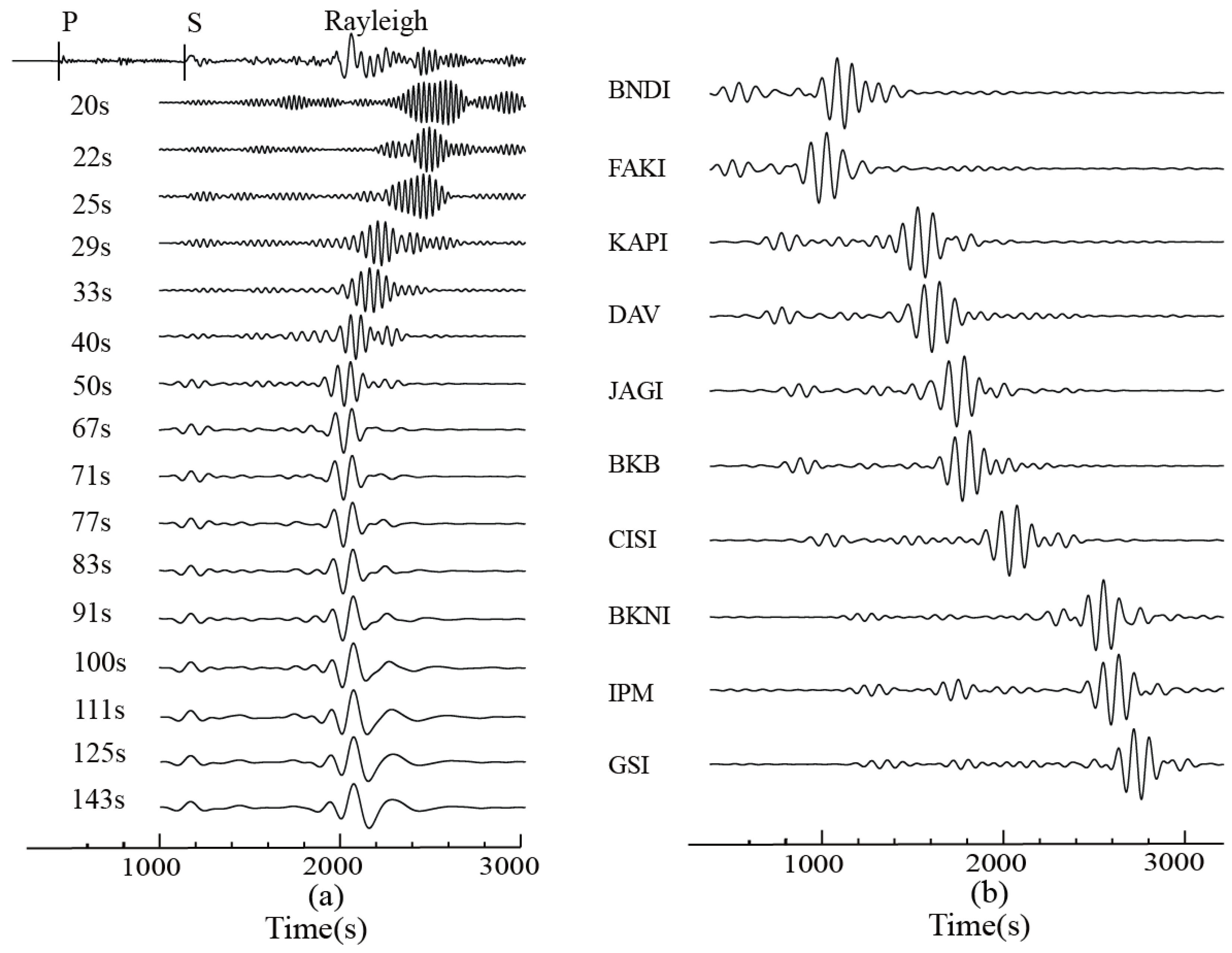
Figure 4.
(a) Example lines show NCFs for station-station pair. (b) Path coverage example of correlation at period of 33s.
Figure 4.
(a) Example lines show NCFs for station-station pair. (b) Path coverage example of correlation at period of 33s.
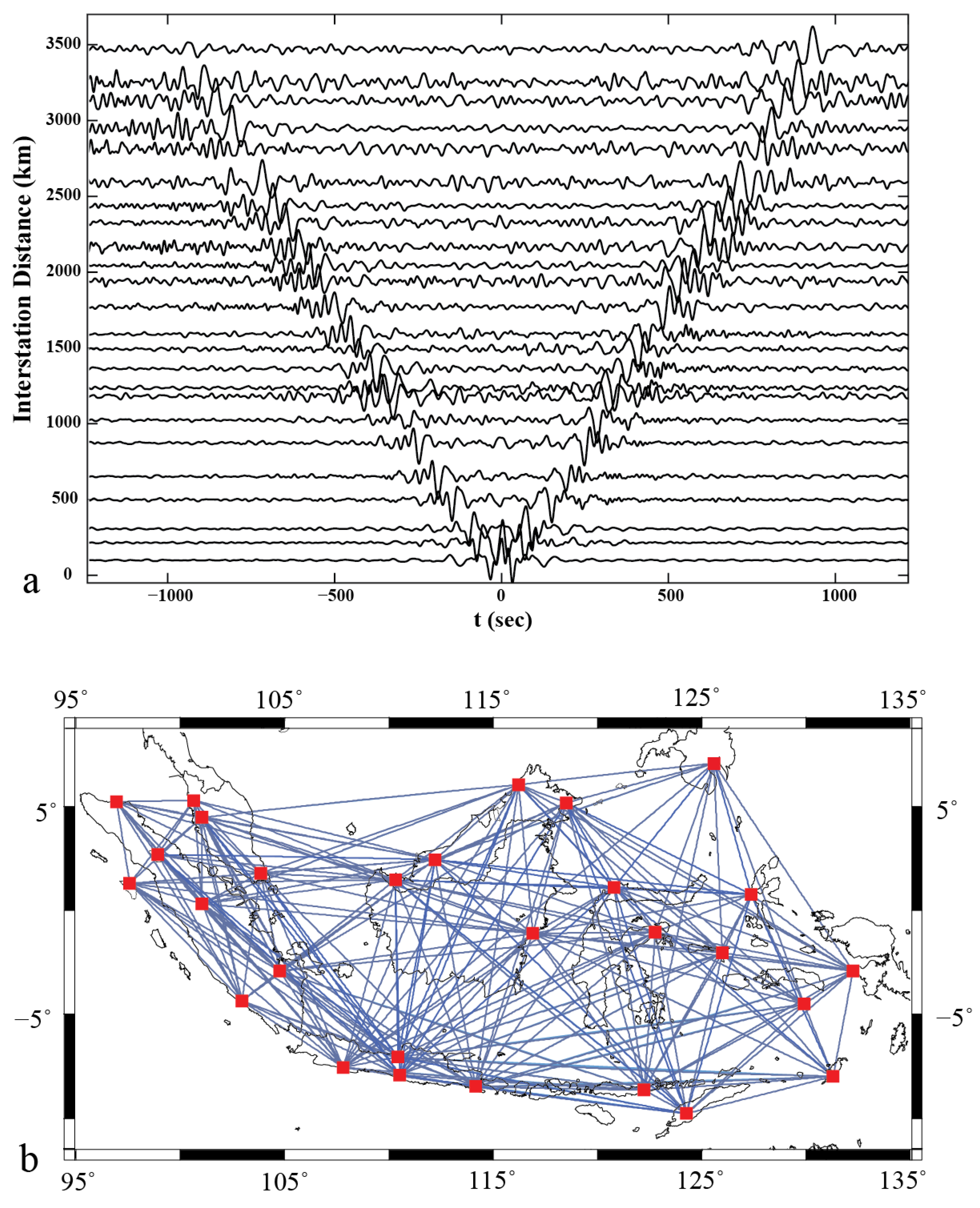
Figure 5.
Checkerboard resolution tests and maps of twice the standard error for phase velocity inversions. Resolution checkboard test and map of 2x standard errors of the phase velocityf inversions. (a) Input model with ±4% velocity perturbations on an 8°×8° grid. (b, d, f) Recovered checkerboard patterns from Rayleigh wave tomography at periods of 33 s, 50 s, and 77 s, shown only where the 2x standard error < 0.08 km/s. (c, e) Recovered patterns from ambient-noise tomography at 33 s and 50 s, clipped to the area of raypath coverage. (g) Map of 2x standard errors at 33 s for ambient noise tomograph. (h) Map of 2x standard errors at 50 s for Rayleigh wave tomography. The white contours outline the smoothed curve of 0.12 km/s (ambient noise) and 0.08 km/s (Rayleigh wave) , respectively.
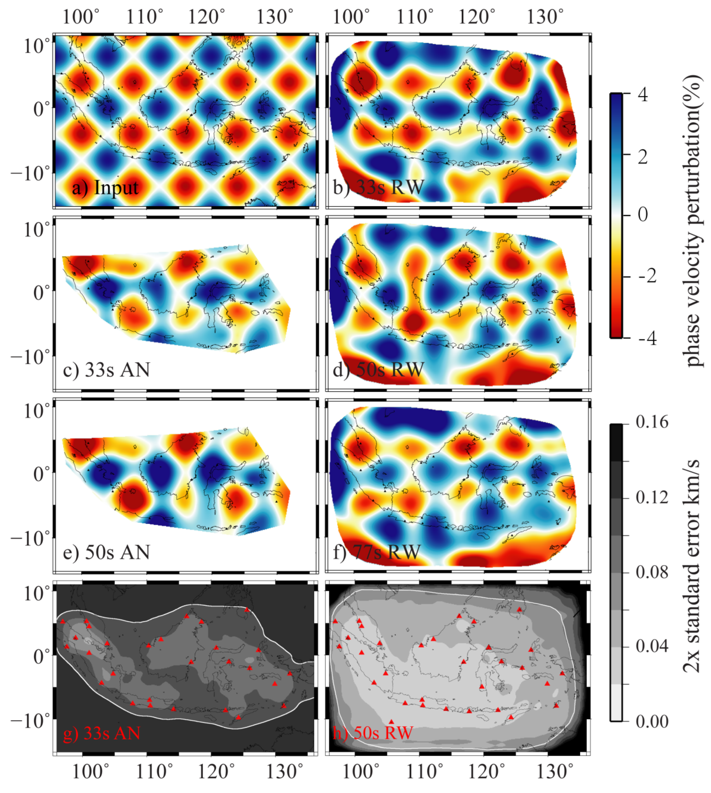
Figure 6.
Mapviews of 2-D phase velocity perturbation at periods of 33s, 40s, 50s, 77s from Ryleigh wave data (the left column) and ambient noise data (the right column).
Figure 6.
Mapviews of 2-D phase velocity perturbation at periods of 33s, 40s, 50s, 77s from Ryleigh wave data (the left column) and ambient noise data (the right column).
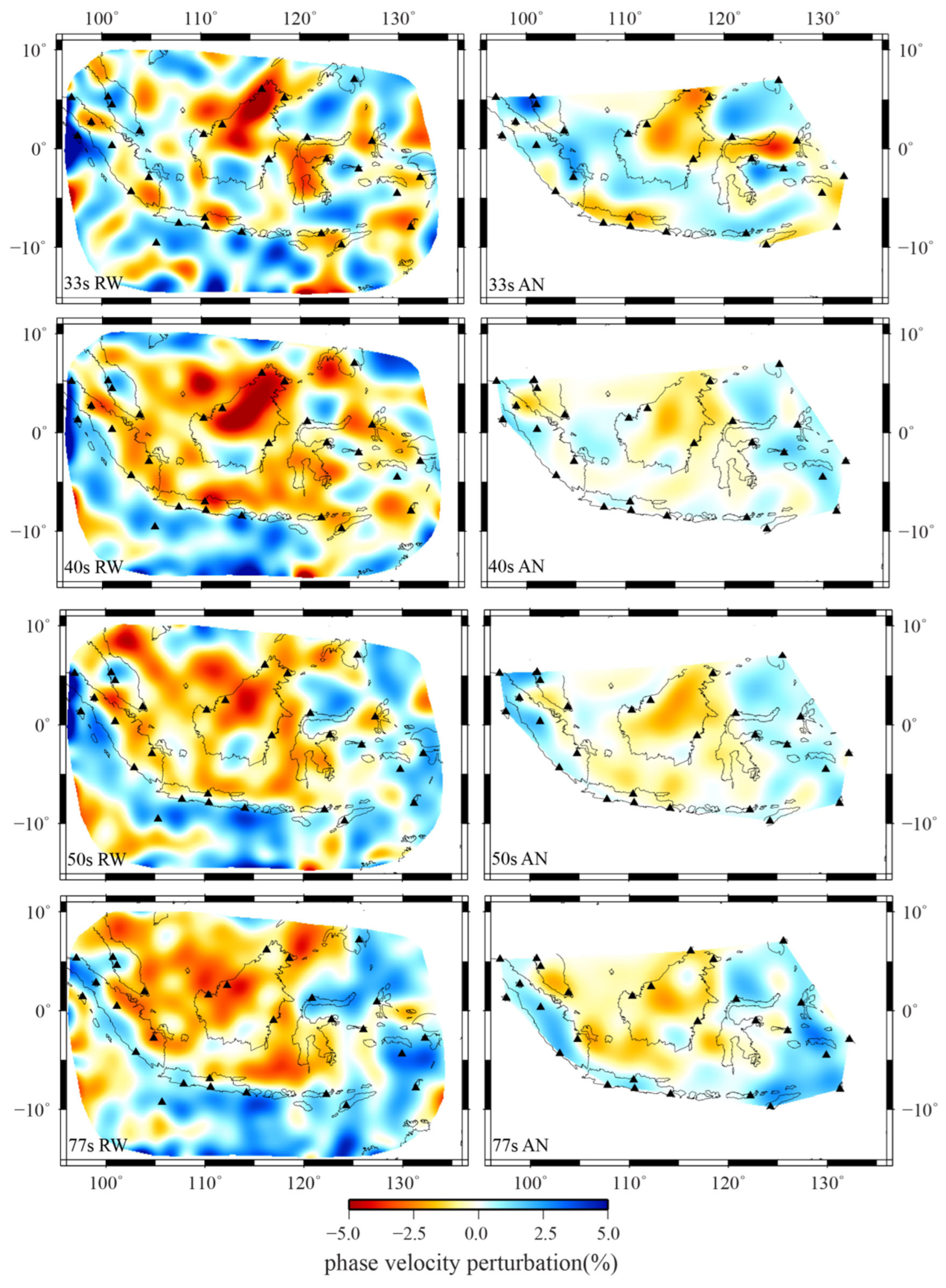
Figure 7.
Mapviews of velocity structure at depths of 40km, 55km, 70km and 90km from Rayleigh wave data (left column), ambient noise data (middle column), and joint periods from 20s to 50s of both data (right column).
Figure 7.
Mapviews of velocity structure at depths of 40km, 55km, 70km and 90km from Rayleigh wave data (left column), ambient noise data (middle column), and joint periods from 20s to 50s of both data (right column).
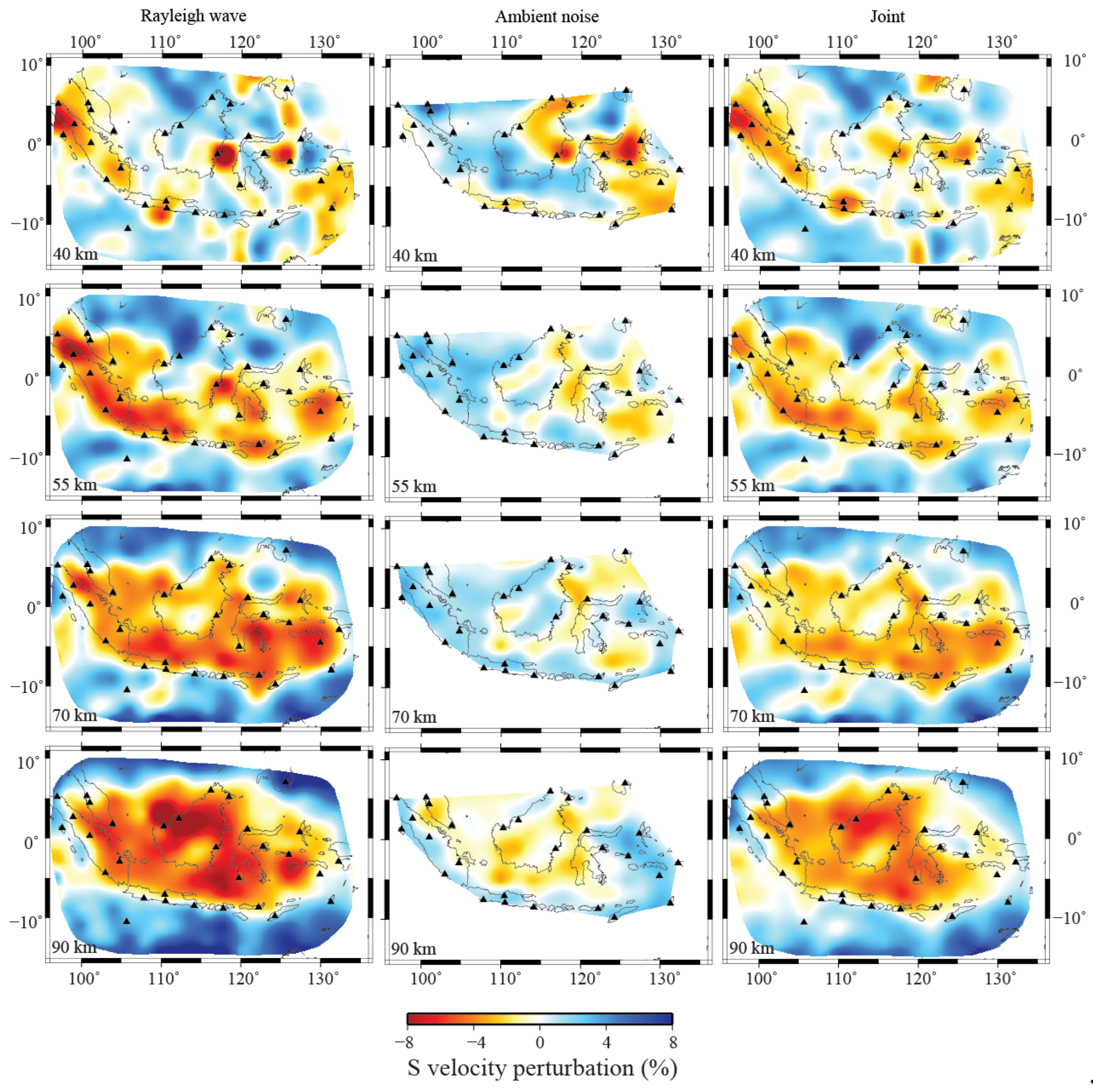
Figure 9.
Seven vertical cross-sections of the 3-D shear wave velocity structure cross major subduction zones with seismicity information. Black dots are earthquakes (MS > 5.0) from USGS since 1985 projected to the section from a perpendicular distance of 1°. Major subduction trenches and seismicity are marked on the map at the right.
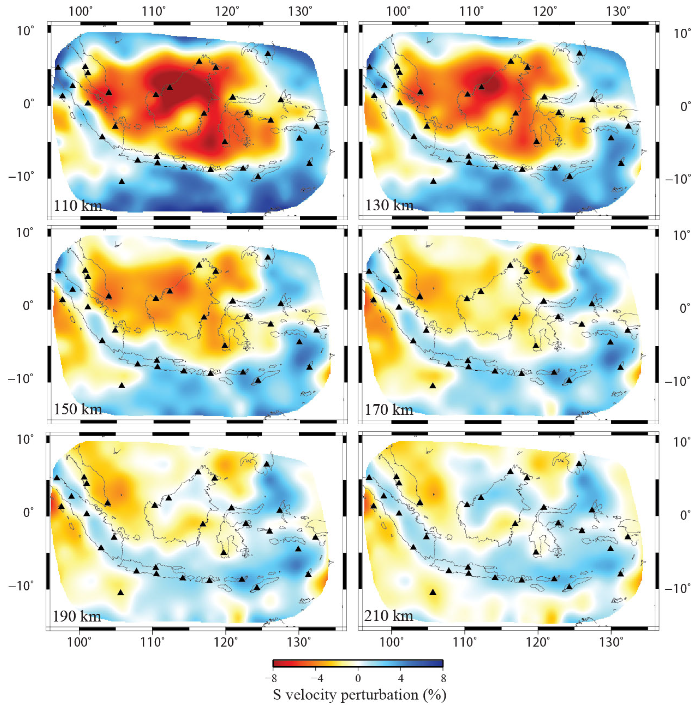
Figure 8.
Mapviews of velocity structure at depths of 110km, 130km, 150km, 170km, 190km and 210km from Rayleigh wave data.
Figure 8.
Mapviews of velocity structure at depths of 110km, 130km, 150km, 170km, 190km and 210km from Rayleigh wave data.
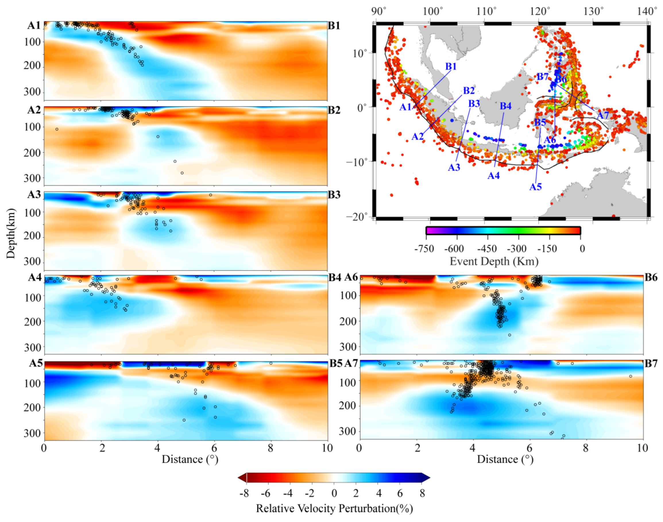
Figure 10.
2.5% high-velocity anomaly 3-D isosurface and six vertical cross-section shear wave velocity structure cross Banda Arc with seismicity information.
Figure 10.
2.5% high-velocity anomaly 3-D isosurface and six vertical cross-section shear wave velocity structure cross Banda Arc with seismicity information.
Disclaimer/Publisher’s Note: The statements, opinions and data contained in all publications are solely those of the individual author(s) and contributor(s) and not of MDPI and/or the editor(s). MDPI and/or the editor(s) disclaim responsibility for any injury to people or property resulting from any ideas, methods, instructions or products referred to in the content. |
© 2026 by the authors. Licensee MDPI, Basel, Switzerland. This article is an open access article distributed under the terms and conditions of the Creative Commons Attribution (CC BY) license (http://creativecommons.org/licenses/by/4.0/).
Copyright: This open access article is published under a Creative Commons CC BY 4.0 license, which permit the free download, distribution, and reuse, provided that the author and preprint are cited in any reuse.


