
Submitted:
05 January 2026
Posted:
07 January 2026
You are already at the latest version
Abstract
Lava flows represent complex thermofluid phenomena in which surface cooling leads to the formation of a solidified surface layer. Understanding the influence of such a surface layer on fluid flow is an important issue in lava flow modeling, and it also shares essential characteristics with a wide range of engineering problems involving surface solidification. However, the role of plastic surface skin in controlling flow deceleration and stopping behavior has not been sufficiently clarified in existing models.
In this study, two-dimensional smoothed particle hydrodynamics (SPH) simulations were conducted to investigate the influence of surface skin formation on lava flow dynamics. The temperature dependence of viscosity was introduced to reproduce a plastic surface skin.
The skin was represented as a low-temperature, high-viscosity region.
Comparisons with simulations without surface skin formation demonstrated that the surface skin exhibits a suppressive effect on the flow. This behavior was consistent with qualitative observations of flowing lava. It was also found that this surface skin caused the successive deceleration characteristic in Bingham fluids. As a result, both the flow velocity and the flowing distance are affected. These results suggest that accurate lava flow simulations require models that incorporate both surface skin effects and non-Newtonian behavior.
Keywords:
lava flow
; surface solidified layer
; surface skin
; non-newtonian fluid
; free-surface flow
; smoothed particle hydrodynamics (SPH)
; particle method
1. Introduction
Lava flows represent complex thermofluid phenomena in which a solidified surface layer forms as a result of surface cooling during flow. Understanding the influence of such a solidified surface layer on fluid flow is a fundamental problem, not only in geophysical contexts but also in a wide range of engineering applications. In mechanical engineering, similar phenomena are exemplified by the formation, deformation, and fracture of solidification shells and thin surface skins in continuous casting. Related surface-solidification phenomena are also observed in welding processes, where thin solidified layers can appear on the surface of molten pools and are associated with weld surface formation [1]. These geophysical and engineering phenomena share essential characteristics.
In lava flows, it is known that two types of solidified surface layers are formed depending on the surface cooling conditions [2]. When the cooling rate is high, the lava surface undergoes supercooling and becomes an amorphous glass. As a result, a thin solidified layer (skin) is formed, which deforms plastically. On the other hand, when the cooling rate is low, crystallization progresses and a rigid solidified layer (crust) is formed.
Based on observations of flowing lava, Hon et al. [3] described the advance of lava accompanied by the skin and the crust. The advance is interpreted as a repeated sequence of the processes outlined below. Initially, a plastically deformable skin with a thickness of approximately 1–2 mm forms on the lava surface. This skin retains the high-temperature lava inside and suppresses its motion. As the flow velocity decreases and cooling progresses further, a rigid crust begins to grow from the skin. When the crust thickness reaches several centimeters, it becomes strong enough to halt the incoming lava. Subsequently, when the crust is locally broken due to an increase in internal pressure, the interior lava flows out again, and the surface returns to a state without a solidified layer.
Furthermore, the rheological properties of lava flows are known to change from Newtonian to non-Newtonian behavior due to the presence of crystals and bubbles within the lava [4]. It has been reported that silicate melts and lavas with a low crystal fraction can be treated as Newtonian fluids over a wide range of temperatures and strain rates [5,6]. On the other hand, lavas with a high crystal fraction exhibit Bingham behavior with a finite yield stress [2]. This change in rheological properties has a significant influence on lava flow dynamics. In addition, lava is also a glass-forming liquid that forms an amorphous glass upon rapid cooling. Its viscosity shows a strong temperature dependence near the glass transition temperature [7].
For the mitigation of damage caused by lava flows, accurate prediction of lava flow behavior is an important social demand. Many previous studies have focused on lava properties and characteristic flow phenomena. These factors must be appropriately incorporated into predictive models. In the context, numerous studies have been conducted on lava flows using a variety of approaches, including field studies [3,5,6,7,8,9,10,11], experimental modeling [4,12,13,14], and numerical simulations [15,16,17,18,19,20,21,22,23,24,25].
Field studies include observations of lava flow behavior and cooling processes [3], as well as analyses of the rheological properties of remelted samples of solidified lava [7,8]. In addition, direct measurements of flowing lava have been conducted to evaluate rheological properties, surface temperature, and flow velocity [9]. However, due to the low frequency of eruptions accompanied by lava flows and the complexity of the phenomena, there are limitations to achieving a comprehensive understanding based only on field observations.
Therefore, analog experiments and numerical simulations play an important role in the study of lava flows. In analog experiments, polyethylene glycol (PEG) is often used to model lava. The materials can reproduce the formation of a rigid crust associated with surface cooling [12,13,14]. Based on these analog experiments, Lyman et al. [13,14] extended the similarity solution for viscosity-dominated gravity currents proposed by Huppert [26]. They incorporated non-Newtonian behavior and introduced the formation of a surface crust as a stopping condition for the flow. On the other hand, these models do not account for the influence of a plastic surface skin on flow behavior.
In numerical simulations, models based on the shallow water equation are widely used in operational forecasting of lava inflow areas [15]. Because these equation treats velocity and temperature distributions as depth-averaged quantities, it is difficult to directly represent phenomena that involve vertical structure, such as viscosity changes associated with surface cooling and the formation of a solidified surface layer.
Phase changes by cooling and deformation of solid–liquid interfaces complicate numerical simulations. For this reason, several previous studies have proposed simplified models for heat transport and phase change. For example, Starodubtsev et al. [18,19] represented solidification behavior indirectly by introducing a time-dependent viscosity model, without solving heat transport. In addition, mesh-based computational methods such as finite volume and finite element methods have the disadvantage of requiring remeshing to accurately treat the deformation of the solid–liquid interface [16,17]. In contrast, smoothed particle hydrodynamics (SPH) which is one of mesh-free particle methods, is well suited for simulating flows with phase change and free surfaces. Despite this advantage, only a few studies have reported lava flow simulations that consider heat transport and solidification using particle methods [20,21,22,24,25].
Hérault et al. [24] conducted lava flow simulations for the actual topography of Mt. Etna, considering heat transport, temperature-dependent viscosity, and non-Newtonian rheology. Through qualitative comparisons with observed volcanic landforms and numerical results, they demonstrated the necessity of modeling lava flows as non-Newtonian fluids with temperature-dependent viscosity. However, this study did not provide a detailed discussion of the specific shapes or formation processes of characteristic lava flow structures, such as lava levees and lava accumulations. Tomita et al. [25] conducted SPH simulations of lava flows using molten metal as an analog material. Under simplified conditions, they successfully reproduced the morphology of characteristic lava flow structures and discussed their geometrical features. Nevertheless, previous studies [20,21,22,24,25] have not sufficiently considered the formation of a surface skin or its influence on flow behavior.
Therefore, the objective of this study is to clarify the influence of the plastic surface skin on lava flow behavior. In this study, two-dimensional SPH simulations are conducted to analyze the flow of a virtual fluid representing lava. The fluid flows down on a horizontal plate while forming a plastically deformable surface skin. The plastic surface skin is represented as a low-temperature, high-viscosity region, through the introduction of a temperature-dependent viscosity.
2. Computational Method
2.1. Governing Equations
In this study, the computational object is the lava flow over a horizontal flat plate with cooling from the surroundings. The thermofluid behavior is described by the continuity equation, the Navier–Stokes equation, and the enthalpy transport equation. The continuity equation for a flow with constant density is given by
where is the velocity. For a fluid with constant density, the Navier–Stokes equation in Lagrangian form is written as
where t is the time, is the density, p is the pressure, is the viscosity, and denotes the gravitational acceleration. Here, the superscript T denotes the transpose of a tensor, and the operator ⊗ represents the tensor product. The Lagrangian form of the enthalpy transport equation is given by
where h is the specific enthalpy, is the thermal conductivity, T is the temperature, and Q denotes the heat loss term, which includes radiative heat loss and heat loss to the ambient air. Assuming that the specific enthalpy depends only on temperature and using specific heat at constant pressure , Equation (3) can be rewritten as the following temperature evolution equation:
2.2. Discretization of Governing Equations in SPH Method
2.2.1. Treatment of Physical Quantities and Differential Operators in SPH
In the SPH method, a physical quantity at the position is evaluated by taking into account the contributions from the neighboring particles b. Defining the relative position vector from position a to position of particle b as , the can be expressed as follows [27]:
where m is the particle mass, and W is the kernel function that represents the spatial distribution of the physical quantity carried by each particle. The kernel value is determined by the distance between points a and b and the particle diameter H. In the following, the notation is used. In this study, the M4 spline function for a two-dimensional space was used as the kernel function [27].
Furthermore, the most fundamental model for the gradient of a physical quantity is obtained by differentiating the kernel function in Equation (5), and is expressed as follows [27]:
where denotes the gradient of the kernel function, which is given by
In addition, the Laplacian of a physical quantity is modeled using the gradient of the kernel function, , as follows [28]:
2.2.2. Discretization of Navier–Stokes Equation
In the SPH method used in this study, the continuity equation does not need to be explicitly solved because mass conservation is satisfied when the particle masses and the total number of particles in the computational domain are constant. Therefore, only the Navier–Stokes equation and the enthalpy transport equation were solved.
By applying the SPH discretization to Equation (2), the following form is obtained:
The first term on the right-hand side of Equation (9) represents the pressure gradient, which is discretized in SPH to satisfy the action–reaction law for each interacting particle pair. This term was replaced by the incompressibility algorithm proposed by Shigeta et al. [29], in order to represent incompressible fluid behavior.
The second term on the right-hand side is the viscosity term. In this simulation, the viscosity is varied in both space and time. In such cases, the Navier–Stokes equation must be discretized without assuming a constant viscosity over the computational domain. However, this leads to more complicated discretization. Therefore, this study adopted the scheme proposed by Morris et al. [30], which can take into account for spatio-temporal variations in viscosity.
In this scheme, the viscosity is initially assumed to be constant, and the term is discretized using the SPH Laplacian model presented in Equation (8),
Subsequently, the viscosity in Equation (10) is redefined as the mean viscosity of the two interacting particles.
The mean value was evaluated using the harmonic mean, in order to treat the large spatial gradients of viscosity.
2.2.3. Discretization of Enthalpy Transport Equation
By applying the SPH discretization to Equation (4), the following form is obtained:
where is the number of spatial dimensions, is the weighted average of the squared values of distances to neighboring particles within the influence radius, and n denotes the particle number density. The first term on the right-hand side represents heat conduction, which is discretized using the Laplacian model of the Moving Particle Semi-implicit (MPS) method [31]. In the SPH method, the Laplacian is represented as a summation of the gradients of kernel functions, which tends to underestimate its value near the surface. On the other hand, in the MPS formulation, the Laplacian is evaluated by taking a weighted average of the kernel functions as a weighting function, which is expected to reduce the underestimation near the surface. The second term on the right-hand side is the heat loss term. According to the previous study by Keszthelyi et al. [10], heat flux due to atmospheric convection and thermal radiation play a dominant role in the cooling of the lava surface. Therefore, likewise in this study, the heat flux to the ambient air and the radiation on the surface are considered as the heat loss rate
These effects were applied only to the surface particles. To identify the surface particles, the method proposed by Ito et al. [32] was used. For a surface particle, neighboring particles are unevenly distributed within the influence radius. As a result, the number-density-based center shifts from the actual particle position toward the interior of the fluid. The magnitude of this displacement is computed as
In this simulation, particles with , were classified as surface particles.
The heat flux to the ambient air is formulated as follows:
where S is the cross-sectional length of a particle, V is the area of the computational particle in the 2D simulation, denotes the distance from the surface to air phase, and is the radius of a computational particle. The subscript "" represents a physical quantity associated with the ambient air. Figure 1 illustrates the concept of this formulation. This equation is derived by assuming that the heat flux from the particle center (point C in Figure 1) to the particle surface (point B) is equal to the heat flux from the particle surface (point B) to the air phase (point A) , and by formulating these conditions as simultaneous equations for the particle surface temperature.
The heat loss due to radiation is expressed by the Stefan–Boltzmann law as follows:
where is the emissivity and is the Stefan–Boltzmann constant.
In this simulation, solidification was modeled by increasing the viscosity depending on its temperature. This treatment captures the plastic behavior of the cooling-induced amorphous glassy surface skin. The formulation and material parameters of the temperature-dependent viscosity are described in detail in Section 2.3.1.
2.3. Computational Conditions
Figure 2 shows the computational domain. In this figure, brown and red areas represent the locations of solid and liquid particles, respectively. A rectangular container with outer dimensions of and a thickness of , was prepared. The origin of the coordinate system was defined at a position in the x-direction and in the y-direction from the lower-left corner of the container. In addition, a horizontal plate was placed in the region and . Then, liquid particles were arranged in a regular lattice within the region and . Figure 2 shows a schematic of the particle configuration at this step. As shown here, the liquid particles are initially accumulated in the lower-left region of the container, which form a dam. Subsequently, a dam-break simulation in which the dam collapsed under gravity acting in the -direction was conducted as a preliminary computation. When the x-directional velocities of all fluid particles converged to , this state was regarded as the initial condition of main simulation. Figure 2 illustrates a schematic of the resulting particle configuration. Finally, in the main computation, the right wall of the container was removed, and the fluid particles flowed onto a horizontal plate, as shown in Figure 2. Inside the container, the fluid was treated as an isothermal fluid at a temperature of . Heat transport was considered only for particles located on the horizontal plate ().
In actual lava flows, the thickness of the surface skin is typically – [3]. If the particle diameter was set sufficiently small to resolve the detailed formation process of such a thin solidified layer, the number of computational particles would become excessively large. Therefore, in this simulation, the effect of skin formation on the overall flow was focused and the particle diameter was set to .
Due to this setting, the particle resolution is relatively coarse. Because heat fluxes due to atmospheric convection and radiative cooling are averaged over the particle area (volume in three-dimensional simulations) at the free surface, the resulting temperature decrease of surface particles cannot be resolved accurately. Accordingly, in order to enhance the temperature response of surface particles and to reproduce skin formation within a feasible computational time, the effects of atmospheric convection and radiation at the surface particles were artificially amplified by a factor of ten.
Furthermore, sufficient temporal resolution was ensured under a feasible computational cost. A time step of was employed throughout the simulation.
In addition, the ambient air temperature was kept constant at , and its thermal conductivity was set to [33]. The distance from the lava surface to the air phase was set equal to the particle radius ().
Table 1 summarizes the computational conditions. The solid phase was assumed to be soil, and its physical properties were taken from the literature [34].
2.3.1. Modeling of Lava Properties
Because lava effusion is commonly observed for low-viscosity basaltic magma, the material properties of liquid particles in this simulation were based on data for basaltic lava. Comprehensive surveys of physical properties conducted within a single volcano are limited. Therefore, data reported in previous studies from various volcanoes were collected.
For the lava density, a constant value of was adopted. It is based on measurements of flowing basaltic lava sampled at Piton de la Fournaise [9].
For the viscosity of lava, experimentally measured values obtained by remelting solidified basaltic lava samples from Mauna Ulu, Kīlauea volcano, were used [7]. In this study [7], the measured viscosity values were fitted using the Vogel–Fulcher–Tammann (VFT) equation and expressed as a function of temperature as follows:
where and T are in and units, respectively. Figure 3 shows the temperature dependence of the viscosity. The blue curve in this figure represents the viscosity calculated based on Equation 17.
Since the rheological behavior of lava flows is consistent with that of a Bingham fluid. As described above, a model used in the simulation should possess the expression of yield stress. Accordingly, an apparent viscosity model [35] was introduced, in which the apparent viscosity is defined as a function of the second invariant of the strain rate tensor given by,
where . The apparent viscosity is expressed as a function of as follows:
where is the reference viscosity, is the yield stress, and is a fitting parameter. This model can express not only the non-Newtonian behavior, but also temperature dependence of viscosity by treating the reference viscosity as a function of temperature.
However, in SPH simulations of viscous fluids, the following stability condition associated with viscosity must be satisfied [28]:
where C denotes a safety factor, and a value of was adopted in this simulation. Under the particle diameter and time step conditions listed in Table 1, the range of viscosity is estimated as from Equation 20.
To satisfy this constraint, in this simulation, the apparent viscosity given by Equation 19 was scaled by a factor of as follows:
where . However, even after this scaling, the apparent viscosity can still exceed the stability threshold by temperature decrease. Therefore, an upper limit of was imposed. In addition, large spatial gradients of viscosity between neighboring particles can lead to numerical instability. Therefore, a lower limit was also introduced, and the viscosity was restricted to the range .
The reference viscosity was represented by the temperature-dependent viscosity of basaltic lava . In Figure 3, the purple curve shows the scaled viscosity, . The scaled reference viscosity was also restricted by the same upper and lower limits, . In Figure 3, the red curve denotes the temperature dependent reference viscosity applied in the simulations with prescribed upper and lower limits. In this simulation, regions where the temperature dependent viscosity were treated as the surface skin. The corresponding temperature for this condition is .
In addition, the yield stress was assumed to be constant at based on values reported in a previous study [24].
For the thermal conductivity and specific heat, temperature-dependent properties of basaltic lava were adopted based on previous studies [10,11].
where , T and are in , and units, respectively.
Based on the formulation of the heat flux to the ambient air described in Equation 15, the following equation corresponds to the heat transfer coefficient :
By substituting the computational conditions and the physical properties of lava and air described above into this equation, the heat transfer coefficient is evaluated as . This value is within the range of experimentally obtained for forced convection in a previous study [10].
The emissivity of lava is generally considered to be [2], and this value was also used in the present study.
Table 2 summarizes the physical properties of basaltic lava used in this study.
In this simulation, four different rheological conditions were considered to evaluate the effects of non-Newtonian behavior and formation of the surface skin on lava flow dynamics. Specifically, four rheological conditions were examined, combining Newtonian or Bingham models with constant or temperature-dependent viscosity (N, TN, B, and TB).
- N: Newtonian fluid with a constant viscosity of
- TN: Newtonian fluid with temperature-dependent viscosity ()
- B: Bingham fluid with a constant reference viscosity of
- TB: Bingham fluid with temperature-dependent viscosity
3. Results and Discussion
3.1. Validation of Numerical Simulations via Comparison with Similarity Solutions
In this study, numerical simulations were considered for a Newtonian fluid with constant viscosity that is instantaneously released onto a horizontal plate. The simulation results are compared with known theoretical scaling laws formulated for viscous-dominated flows [26], as follows:
where L is the flow length, g is the gravitational acceleration, q represents the cross-sectional area of the released fluid. The constant is a dimensionless coefficient determined by the similarity solution [26]. In the case of a two-dimensional flow, . denotes the density difference between the fluid and the ambient medium. In the present simulations, the ambient medium is not modeled. Therefore, is taken as . This assumption is reasonable for lava flows, since .
Figure 4 compares the simulated flow length of condition N with the theoretical solution proposed by Huppert [26]. To compare the simulation results with the theoretical scaling, it is necessary to identify the time range in which the flow is dominated by viscous effects. In actual physical processes, the early stage flow behavior is influenced by inertial slumping, which precedes the viscous-dominated flow [13]. Therefore, this initial transient stage should be excluded from the quantitative comparison.
According to the scaling relation given by Equation 25, the flow length follows in the viscous-dominated flow. When the flow follows the scaling, the quantity becomes constant. Therefore, the compensated quantity is introduced and evaluated to diagnose the transition to the viscous-dominated flow. Figure 5 shows the time evolution of the relative change of the compensated quantity, described as . As time progresses, the magnitude of the relative change decreases. After approximately , the relative change remains at a low level of order . Based on Figure 5, is adopted as the viscous-dominated regime.
For the data within the viscous-dominated regime, the relative root-mean-square error (rRMSE) between the simulation result of condition N and the theoretical solution proposed by Huppert [26] is evaluated. The resulting rRMSE is . This result indicates that the simulation results agree with the theoretical scaling within a relative error of approximately .
In the following analysis, the time exponent is fixed to , and only the constant is treated as a fitting parameter. The value of is determined by minimizing the rRMSE between the simulation result and the theoretical scaling. As a result, the optimal value is found to be , while the theoretical value is . With this optimized prefactor, the rRMSE is reduced to . This result indicates that the temporal scaling predicted by the theory is well reproduced by the simulation.
These results indicate that the numerical simulations show reasonable agreement with the known theoretical scaling laws. This agreement supports the validity of the simulations for the Newtonian condition.
For Bingham fluids, Lyman [13] proposed a theoretical model that describes the final stopping position of a flow front. This model is derived from the static balance between the yield stress and the gravitational driving force. The theoretical stopping length is given by
In this study, the numerical simulation results of condition B are compared with this theoretical prediction, with a focus on the final flow length at stopping.
Figure 6 shows the temporal evolution of the flow front position obtained from the numerical simulation for condition B. The final stopping position predicted by the theoretical model of Lyman [13] is also shown for comparison.
As shown here, the stopping length measured from the origin in the simulation is approximately . In contrast, the theoretical model predicts a stopping length of . The stopping length obtained from the numerical simulation corresponds to approximately of the theoretical prediction. Lyman [13] reported that, for Bingham fluids, the experimentally observed stopping lengths range from to of the theoretical values. In Figure 6, the thin dashed lines indicate this experimentally observed variability range. The result of simulation is within the variability range reported in previous experimental validations.
The result of simulation is within the experimentally observed variability range indicated by the thin dashed lines in Figure 6.
Based on the comparison described above, these results indicate that the numerical simulations show reasonable agreement with the theoretical model for Bingham fluids. This agreement supports the validity of the simulations in capturing the stopping behavior both qualitatively and quantitatively.
3.2. Effects of Bingham Behavior on Flow Deceleration and Distance
Figure 7 shows the time evolution of the flow front position for each condition. The blue, green, orange, and red lines correspond to the conditions N, TN, B, and TB, respectively.
As shown in Figure 7, a clear difference is observed in the approach to the stopped state between Newtonian fluids (N and TN) and Bingham fluids (B and TB). For conditions N and TN, the flow velocity decreases gradually. In contrast, for conditions B and TB, the flow undergoes a rapid decrease in velocity before reaching the stopped state.
Figure 8 shows the velocity distributions in the x-direction for each condition when the flow front reaches . It should be noted that the aspect ratio is changed for visibility in the figures. A difference is observed in the spatial extent of the region with velocities higher than between Newtonian fluids (conditions N and TN) and Bingham fluids (conditions B and TB). On the other hand, no significant difference is found in this high-velocity region between the two Newtonian conditions (N and TN). A similar result is obtained between the two Bingham conditions (B and TB).
Figure 9 shows the velocity distributions in the x-direction for each condition when the flow front reaches . The Bingham fluids (Figure 9 and Figure 9) exhibit lower velocities than the Newtonian fluids (Figure 9 and Figure 9). The region with velocities higher than disappears in the Bingham conditions.
Figure 10 shows the velocity distributions in the x-direction for each condition when the flow front reaches for Newtonian conditions (N and TN) and for Bingham conditions (B and TB). In addition, Figure 11 shows the velocity distributions at when the flow under condition N reaches the domain boundary. A comparison between Figure 10 and Figure 11 for condition TB shows that the flow front exhibits almost no further displacement. This observation allows the Bingham flows under condition TB to be regarded as stopped at the final stage. In particular, as shown in Figure 10, the flow under condition TB has already lost most of its velocity at .
Figure 12 shows the apparent viscosity distributions for conditions B and TB when the flow reaches at and . Here, the apparent viscosity distribution under condition TB at (Figure 12) is compared with that at (Figure 12), where the flow is still advancing. This comparison shows that the apparent viscosity increases over the entire flow region during this time. A similar comparison is conducted for condition B. The apparent viscosity distribution at (Figure 12) is compared with that at (Figure 12). The increase in the apparent viscosity is found to start from the upstream region.
Figure 12 and Figure 12 are compared with the velocity distributions at the same times (Figure 9 and Figure 10). The upstream region exhibits lower velocities than the downstream region. This observation indicates that the apparent viscosity increases in regions where the flow velocity decreases.
Therefore, a feedback process within the Bingham fluid model is suggested. A decrease in flow velocity reduces the velocity gradient. This reduction leads to an increase in the apparent viscosity. The increased apparent viscosity further decreases the flow velocity. The repetition of this process can cause a rapid decrease in velocity and eventually lead to a stopping of the flow.
Through this feedback process, the simulation captures behavior that is consistent with the characteristics of a Bingham fluid. In actual Bingham fluids, a decrease in the velocity gradient causes the shear stress to fall below the yield stress. As a result, the fluid exhibits solid-like behavior.
In this simulation, the Bingham fluid behavior was confirmed to have an influence on the flow deceleration and on the flowing distance. These results are consistent with the understanding [24] that non-Newtonian fluid models are required for accurate prediction of lava flow behavior.
3.3. Effects of Skin Formation on Flow Deceleration and Distance
As shown in Figure 7, the time evolution of the flow front position indicates that conditions N and TN exhibit similar gradual deceleration trends. However, at the same elapsed time for both conditions, condition TN exhibits a shorter flowing distance than condition N. This difference in flowing distance is found to increase as time progresses.
Similarly, conditions B and TB exhibit similar abrupt deceleration trends. However, at the same elapsed time for both conditions, condition TB exhibits a shorter flowing distance than condition B. As a result, the final stopping distance under condition TB is smaller than that under condition B.
Figure 8, Figure 9, Figure 10 and Figure 11 show the velocity distributions in the x-direction for four conditions. First, the velocity distributions of the two Newtonian fluids under conditions N and TN are compared. When the flow front reaches (Figure 8 and Figure 8), the velocity distributions under conditions N and TN are similar. When the flow front reaches (Figure 9 and Figure 9), the spatial extent of the region with velocities between and is smaller under condition TN than under condition N. When the flow front reaches (Figure 10 and Figure 10), the difference in velocity between conditions N and TN becomes more pronounced.
Similarly, the velocity distributions of the two Bingham fluids under conditions B and TB are compared. When the flow front reaches (Figure 8 and Figure 8), the velocity distributions under conditions B and TB are similar, as in the Newtonian conditions. When the flow front reaches (Figure 9 and Figure 9), the velocity under condition TB is lower overall than that under condition B. When the flow front reaches (Figure 10 and Figure 10), the flow under condition TB has lost most of its velocity, and the front position shows almost no further change, even at (Figure 11). On the other hand, at (Figure 10), the flow under condition B continues to advance. At , the front position under condition B (Figure 11) is located further downstream than that under condition TB (Figure 11).
Figure 13 shows the apparent viscosity distributions at the time when flows reach at for each condition. Under the temperature-dependent conditions TN (Figure 13) and TB (Figure 13), a high-viscosity region with is observed at the flow surface.
Figure 14 shows the temperature distributions at the time when flows reach at for conditions TN and TB. A comparison between Figure 13 and Figure 14 indicates that this surface region satisfies and . A similar relationship between the apparent viscosity (Figure 13) and temperature (Figure 14) is also observed in the condition TB. This result shows that the surface layer is represented as a low-temperature, high-viscosity skin.
Figure 13 for condition N and Figure 13 for condition TN show that the scaled viscosity inside the flow is mostly lower than . This observation indicates that cooling-induced skin formation occurs only at the flow surface.
Similarly, Figure 13 for condition B and Figure 13 for condition TB show comparable viscosity distributions inside the flow. This result indicates that skin formation due to cooling is confined to the flow surface, even for the Bingham fluid conditions.
On the other hand, Figure 12 and Figure 12 show the apparent viscosity distributions when the flow fronts reach . At this stage, Figure 12 and Figure 12 indicate that the apparent viscosity inside the flow is overall higher under condition TB than under condition B. This result suggests that the velocity reduction process associated with Bingham behavior occurs at a shorter flowing distance under condition TB than under condition B.
From the above comparisons of the velocity distributions and the time evolution of the flow front positions, the effects of the surface skin are examined for both the Newtonian conditions (N and TN) and the Bingham conditions (B and TB). These results indicate that the cooling-induced surface skin suppresses the flow and reduces the flow velocity. This interpretation is consistent with qualitative observations of lava flows. In such flows, a plastically deformable surface skin formed at the flow surface retains the internal lava near the flow front [3].
Under condition TN, the suppression of the flow by the surface skin causes the flow to exhibit longer arrival times at corresponding positions than under condition N. Similarly, under condition TB, the surface skin causes the Bingham related velocity reduction to occur at a shorter flowing distance than under condition B. As a result, this behavior leads to a difference in the final stopping position of the flow.
These results suggest that surface skin formation plays a role in the flow characteristics of lava flows, and that accurate simulation of lava flow behavior requires viscosity models that appropriately account for both non-Newtonian behavior and skin formation.
4. Conclusions
The objective of this study was to clarify the influence of the plastic surface skin on lava flow behavior. To this end, two-dimensional SPH simulations were conducted to analyze the flow of a lava-inspired virtual fluid on a horizontal plate. The surface skin was represented as a low-temperature, high-viscosity region through the introduction of a temperature-dependent viscosity. The flow behavior was evaluated by comparing conditions with and without non-Newtonian (Bingham) behavior and with and without surface skin formation.
The main conclusions of this study are summarized as follows:
- 1.
- The numerical results obtained for the isothermal Newtonian condition showed reasonable agreement with established theoretical solution [26] in terms of the time evolution of the flow. In addition, the results for the isothermal Bingham condition were consistent with theoretical prediction [13] regarding the final stopping position of the flow. These agreements support the validity of the present simulation framework for describing viscous-dominated and yield-stress-controlled flow behavior.
- 2.
- By introducing the apparent viscosity model, it was confirmed that the apparent viscosity increases as the flow velocity decreases. This increase in apparent viscosity further reduces the flow velocity and eventually leads to the stopping of the lava flow. This behavior qualitatively reproduces the characteristics of a Bingham fluid. As a result, the flow velocity and the flowing distance are affected. These results are consistent with the prevailing understanding that non-Newtonian fluid models are required for accurate prediction of lava flowing distances.
- 3.
- By considering the temperature dependence of viscosity, a plastic surface skin was successfully reproduced in the numerical simulations. Comparison with simulations without surface skin formation revealed that the surface skin reduces the flow velocity. This behavior is consistent with qualitative observations [3]. In particular, when Bingham behavior is taken into account, the suppressive effect of the surface skin causes the successive deceleration characteristic in Bingham fluids, as described above, to emerge at a shorter flowing distance. Therefore, these results suggest that accurate prediction of lava flowing distances requires models that incorporate both non-Newtonian behavior and surface skin formation.
These present findings highlight the importance of surface skin formation in lava flow dynamics. Similar physical considerations are also relevant to engineering and other thermofluid systems involving surface solidification. Future work will focus on extending the present model to incorporate realistic thermophysical properties of actual lava and to evaluate the quantitative influence of surface skin formation at natural flow scales. In particular, a semi-implicit treatment [22,36] of the viscous term will be introduced to relax the severe time step restriction caused by high viscosity. Such developments are expected to contribute to more accurate prediction of lava flow behavior.
Author Contributions
Conceptualization, S.T.; Methodology, S.T.; software, S.T., H.K.; validation, S.T.; formal Analysis, S.T., T.S., S.M., J.Y., M.S. (Makoto Sugimoto), H.K. and M.S. (Masaya Shigeta); investigation, S.T.; discussion, S.T., T.S., S.M., J.Y., M.S. (Makoto Sugimoto), H.K. and M.S. (Masaya Shigeta); writing—original draft preparation, S.T.; writing—review and editing, J.Y., M.S.(Makoto Sugimoto), H.K. and M.S. (Masaya Shigeta); visualization, S.T.; supervision, M.S. (Masaya Shigeta); project administration, M.S. (Masaya Shigeta); resources, M.S.(Makoto Sugimoto), M.S. (Masaya Shigeta); funding acquisition, M.S. (Masaya Shigeta). All authors have read and agreed to the published version of the manuscript.
Funding
This research was funded by Japan Society for the Promotion of Science KAKENHI grant number 25K01152.
Institutional Review Board Statement
Not applicable.
Informed Consent Statement
Not applicable.
Data Availability Statement
The data presented in this study are available upon request from the corresponding author. The data are not publicly available because the data are not required to read the article.
Conflicts of Interest
The authors declare no conflicts of interest.
References
- Yin, X.; Zhang, Y.; Li, B.; Chen, C. Study of the solidified thin layer on molten pool surface in laser deep penetration welding. Optics & Laser Technology 2022, 149, 107842. [Google Scholar] [CrossRef]
- Griffiths, R.W. The Dynamics of Lava Flows. Annual Review of Fluid Mechanics 2000, 32, 477–518. [Google Scholar] [CrossRef]
- Hon, K.; Kauahikaua, J.; Denlinger, R.; Mackay, K. Emplacement and inflation of pahoehoe sheet flows: Observations and measurements of active lava flows on Kilauea Volcano, Hawaii. Geological Society of America Bulletin 1994, 106, 351–370. [Google Scholar] [CrossRef]
- Bokharaeian, M. Rheological study of lava flow analog mixtures. Acta Geodynamica et Geomaterialia 2023, 20, 11–18. [Google Scholar] [CrossRef]
- Dingwell, D.; Webb, S. Structural relaxation in silicate melts and non-Newtonian melt rheology in geologic processes. Physics and Chemistry of Minerals 1989, 16, 508–516. [Google Scholar] [CrossRef]
- Lejeune, A.M.; Richet, P. Rheology of crystal-bearing silicate melts: An experimental study at high viscosities. Journal of Geophysical Research: Solid Earth 1995, 100, 4215–4229. [Google Scholar] [CrossRef]
- Sehlke, A.; Whittington, A.; Robert, B.; Harris, A.; Gurioli, L.; Médard, E. Pahoehoe to àà transition of Hawaiian lavas: an experimental study. Bulletin of Volcanology 2014, 76, 876. [Google Scholar] [CrossRef]
- Ishibashi, H.; Sato, H. Bingham fluid behavior of plagioclase-bearing basaltic magma: Reanalyses of laboratory viscosity measurements for Fuji 1707 basalt. Journal of Mineralogical and Petrological Sciences 2010, 105, 334–339. [Google Scholar] [CrossRef]
- Harris, A.; Mannini, S.; Thivet, S.; Chevrel, M.; Gurioli, L.; Villeneuve, N.; Muro, A.D.; Peltier, A. How shear helps lava to flow. Geology 2020, 48, 154–158. [Google Scholar] [CrossRef]
- Keszthelyi, L.; Denlinger, R. The initial cooling of pahoehoe flow lobes. Bulletin of Volcanology 1996, 58, 5–18. [Google Scholar] [CrossRef]
- Touloukian, Y.; Judd, W.; Roy, R. Physical Properties of Rocks and Minerals; Hemisphere Pub. Corp., 1989. [Google Scholar]
- Miyamoto, H.; Crown, D.A. A simplified two-component model for the lateral growth of pahoehoe lobes. Journal of Volcanology and Geothermal Research 2006, 157, 331–342. [Google Scholar] [CrossRef]
- Lyman, A.W.; Kerr, R.C.; Griffiths, R.W. Effects of internal rheology and surface cooling on the emplacement of lava flows. Journal of Geophysical Research: Solid Earth 2005, 110, 1–16. [Google Scholar] [CrossRef]
- Lyman, A.W.; Kerr, R.C. Effect of surface solidification on the emplacement of lava flows on a slope. Journal of Geophysical Research: Solid Earth 2006, 111. [Google Scholar] [CrossRef]
- Mount Fuji Research Institute Yamanashi Prefectural Government. Kazan Bousai Map no Shinraisei Koujou ni Shisuru Suuchi Simulation Gijutsu no Koudoka (Improvement of Numerical Simulation Techniques for Enhancing the Reliability of Volcano Hazard Maps). (In Japanese). 2024. [Google Scholar]
- Tsepelev, I.; Ismail-Zadeh, A.; Melnik, O.; Korotkii, A. Numerical modeling of fluid flow with rafts: An application to lava flows. Journal of Geodynamics 2016, 97, 31–41. [Google Scholar] [CrossRef]
- Tsepelev, I.; Ismail-Zadeh, A.; Starodubtseva, Y.; Korotkii, A.; Melnik, O. Crust Development Inferred from Numerical Models of Lava Flow and Its Surface Thermal Measurements. Annals of Geophysics 2019, 61, 1–17. [Google Scholar] [CrossRef]
- Starodubtsev, I.; Vasev, P.; Starodubtseva, Y.; Tsepelev, I. Numerical Simulation and Visualization of Lava Flows. Scientific Visualization 2022, 14, 66–76. [Google Scholar] [CrossRef]
- Starodubtsev, I.S.; Starodubtseva, Y.V.; Tsepelev, I.A.; Ismail-Zadeh, A.T. Three-Dimensional Numerical Modeling of Lava Dynamics Using the Smoothed Particle Hydrodynamics Method. Journal of Volcanology and Seismology 2023, 17, 175–186. [Google Scholar] [CrossRef]
- Zago, V.; Bilotta, G.; Cappello, A.; Dalrymple, R.A.; Fortuna, L.; Ganci, G.; Hérault, A.; Negro, C.D. Simulating Complex Fluids with Smoothed Particle Hydrodynamics. Annals of Geophysics 2017, 60. [Google Scholar] [CrossRef]
- Zago, V.; Bilotta, G.; Hérault, A.; Dalrymple, R.A.; Fortuna, L.; Cappello, A.; Ganci, G.; Negro, C.D. Semi-implicit 3D SPH on GPU for lava flows. Journal of Computational Physics 2018, 375, 854–870. [Google Scholar] [CrossRef]
- Zago, V.; Bilotta, G.; Cappello, A.; Dalrymple, R.A.; Fortuna, L.; Ganci, G.; Hérault, A.; Negro, C.D. Preliminary validation of lava benchmark tests on the GPUSPH particle engine. Annals of Geophysics 2019, 61. [Google Scholar] [CrossRef]
- Bilotta, G.; Zago, V.; Centorrino, V.; Dalrymple, R.A.; Hérault, A.; Negro, C.D.; Saikali, E. A numerically robust, parallel-friendly variant of BiCGSTAB for the semi-implicit integration of the viscous term in Smoothed Particle Hydrodynamics. Journal of Computational Physics 2022, 466, 111413. [Google Scholar] [CrossRef]
- Hérault, A.; Bilotta, G.; Vicari, A.; Rustico, E.; Negro, C.D. Numerical simulation of lava flow using a GPU SPH model. Annals of Geophysics 2011, 54, 600–620. [Google Scholar] [CrossRef]
- Tomita, S.; Yoshikawa, J.; Sugimoto, M.; Komen, H.; Shigeta, M. SPH Simulation of Molten Metal Flow Modeling Lava Flow Phenomena with Solidification. Dynamics 2024, 4, 287–302. [Google Scholar] [CrossRef]
- Huppert, H.E. The propagation of two-dimensional and axisymmetric viscous gravity currents over a rigid horizontal surface. Journal of Fluid Mechanics 1982, 121, 43–58. [Google Scholar] [CrossRef]
- Monaghan, J.J. Smoothed Particle Hydrodynamics. Annual Review of Astronomy and Astrophysics 1992, 30, 543–574. [Google Scholar] [CrossRef]
- Asai, M. Meikai Ryushi-ho (Clear Explanation of Particle Methods); (In Japanese). Maruzen Publishing, 2022. [Google Scholar]
- Shigeta, M.; Watanabe, T.; Izawa, S.; Fukunishi, Y. Incompressible SPH Simulation of Double-Diffusive Convection Phenomena. International Journal of Emerging Multidisciplinary Fluid Sciences 2009, 1, 1–18. [Google Scholar] [CrossRef]
- Morris, J.P.; Fox, P.J.; Zhu, Y. Modeling Low Reynolds Number Incompressible Flows Using SPH. Journal of Computational Physics 1997, 136, 214–226. [Google Scholar] [CrossRef]
- Koshizuka, S.; Oka, Y. Moving-Particle Semi-Implicit Method for Fragmentation of Incompressible Fluid. Nuclear Science and Engineering 1996, 123, 421–434. [Google Scholar] [CrossRef]
- Ito, M.; Nishio, Y.; Izawa, S.; Fukunishi, Y.; Shigeta, M. Numerical Simulation of Joining Process in a TIG Welding System Using Incompressible SPH Method. Quarterly Journal of the Japan Welding Society 2015, 33, 34s–38s. [Google Scholar] [CrossRef]
- The Japan Society of Thermophysical Properties. Shinpen Netsu Bussei Handbook (Thermophysical Properties Handbook); (In Japanese). Yokendo, 2008. [Google Scholar]
- The Japan Society of Mechanical Engineers. JSME data book: heat transfer, (In Japanese), 4th ed.; The Japan Society of Mechanical Engineers, 1966. [Google Scholar]
- Papanastasiou, T.C. Flows of Materials with Yield. Journal of Rheology 1987, 31, 385–404. [Google Scholar] [CrossRef]
- Monaghan, J. On the integration of the SPH equations for a highly viscous fluid. Journal of Computational Physics 2019, 394, 166–176. [Google Scholar] [CrossRef]
Figure 1.
Conceptual diagram of heat flux ambient air employed in the formulation.
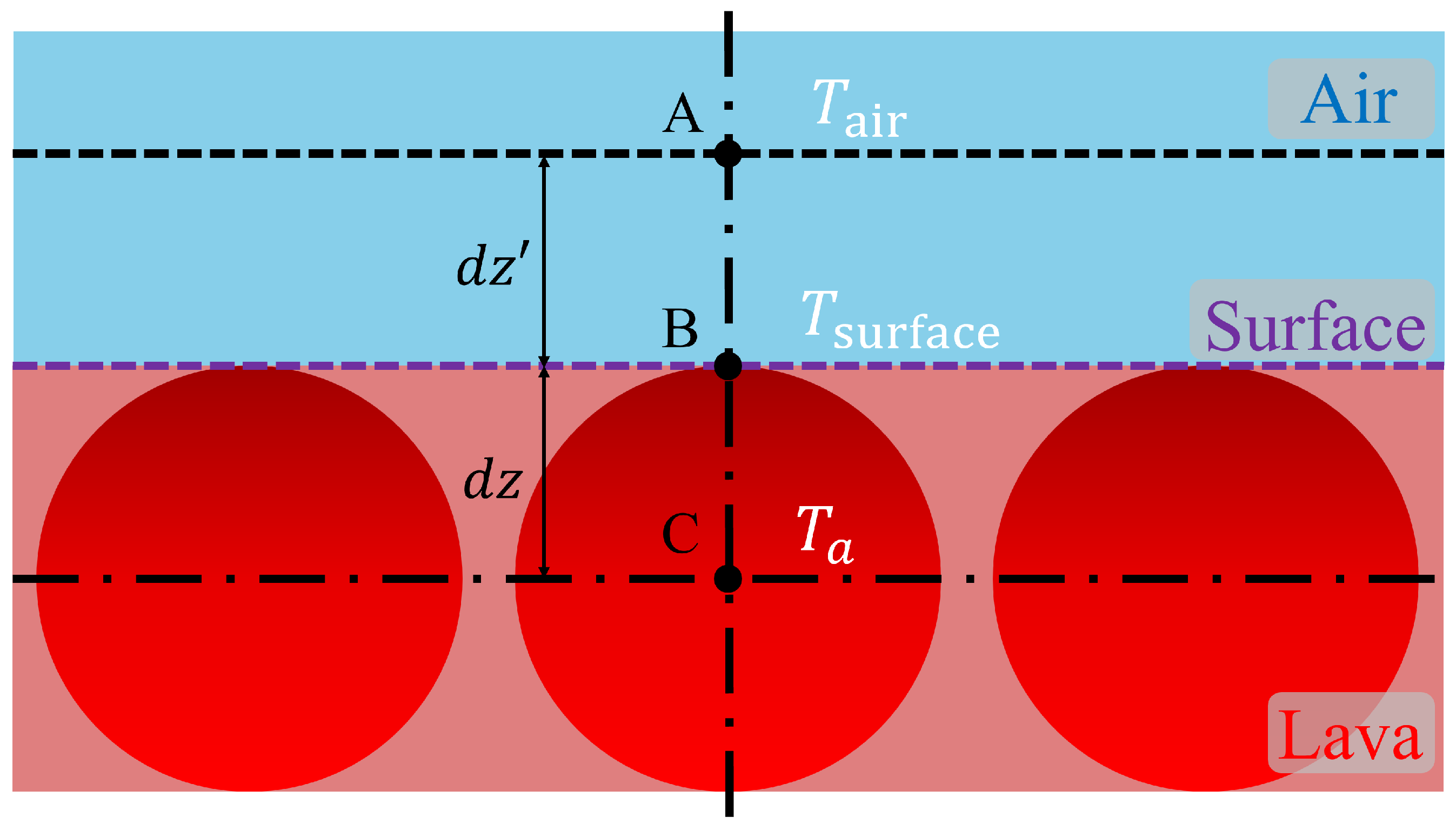
Figure 2.
Computational domain: (a) before the dam-break simulation, (b) at initial condition of lava flow simulation, and (c) after the wall is removed. Brown area represents solid particles, and red area denotes liquid particles.
Figure 2.
Computational domain: (a) before the dam-break simulation, (b) at initial condition of lava flow simulation, and (c) after the wall is removed. Brown area represents solid particles, and red area denotes liquid particles.
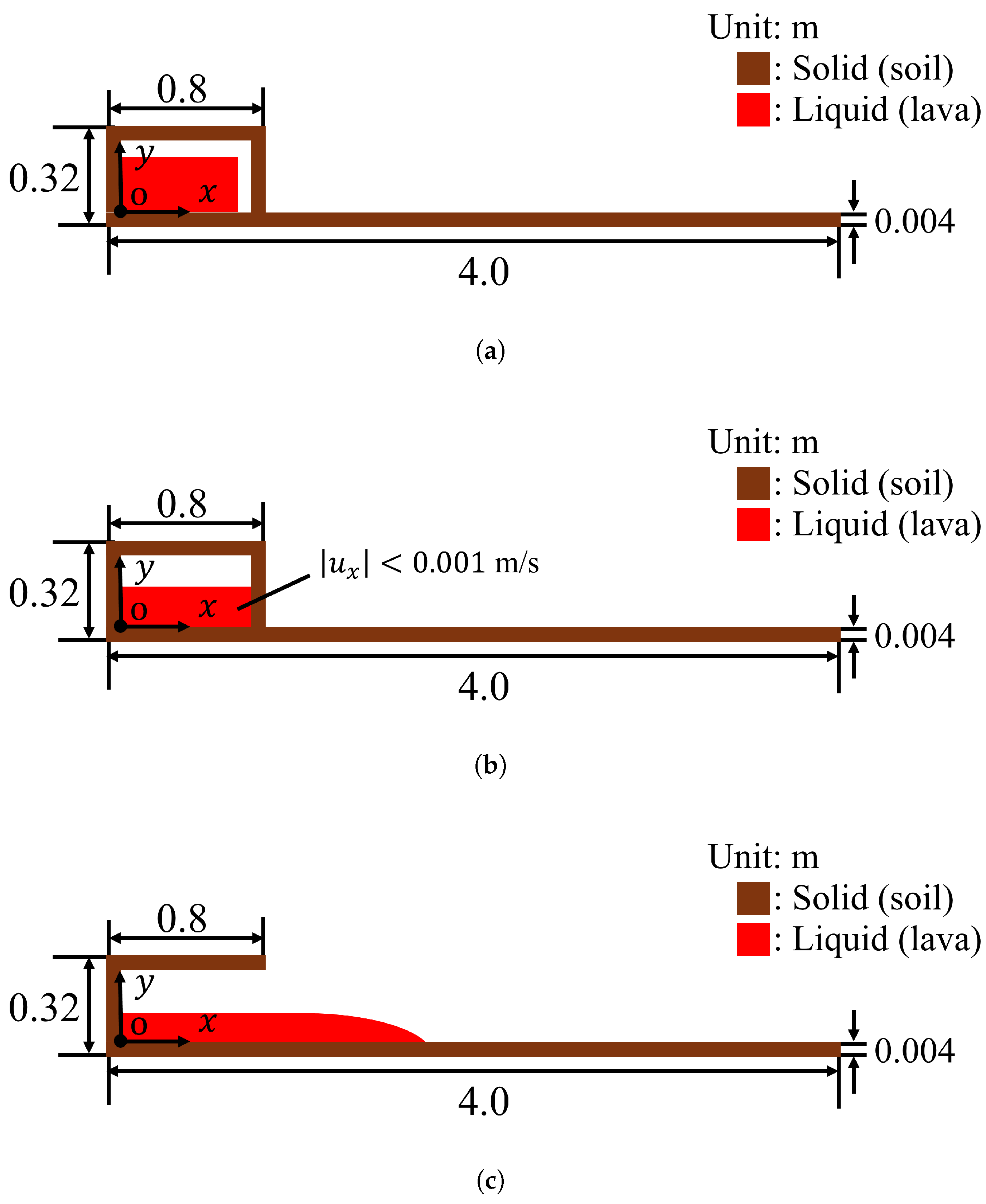
Figure 3.
Temperature dependency of viscosity. The blue curve represents the viscosity of basaltic lava, . The purple curve shows the scaled viscosity, . The red curve, , denotes the temperature-dependent viscosity applied in the simulations with limited range.
Figure 3.
Temperature dependency of viscosity. The blue curve represents the viscosity of basaltic lava, . The purple curve shows the scaled viscosity, . The red curve, , denotes the temperature-dependent viscosity applied in the simulations with limited range.
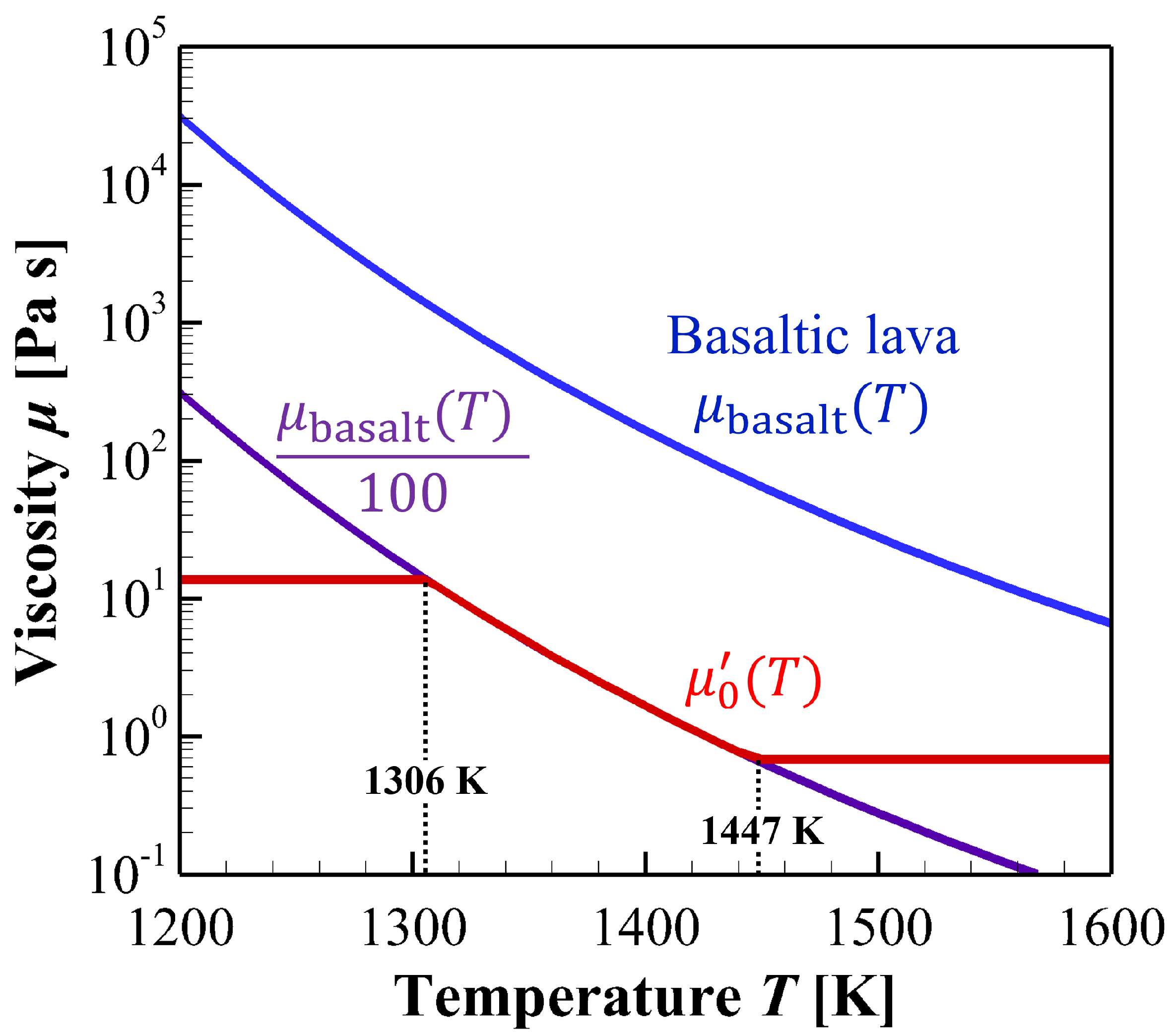
Figure 4.
Comparison of the simulated flow length (condition N) with the theoretical scaling proposed by Huppert [26]. The solid line represents the simulation result, and the dashed line denotes the theoretical solution.
Figure 4.
Comparison of the simulated flow length (condition N) with the theoretical scaling proposed by Huppert [26]. The solid line represents the simulation result, and the dashed line denotes the theoretical solution.
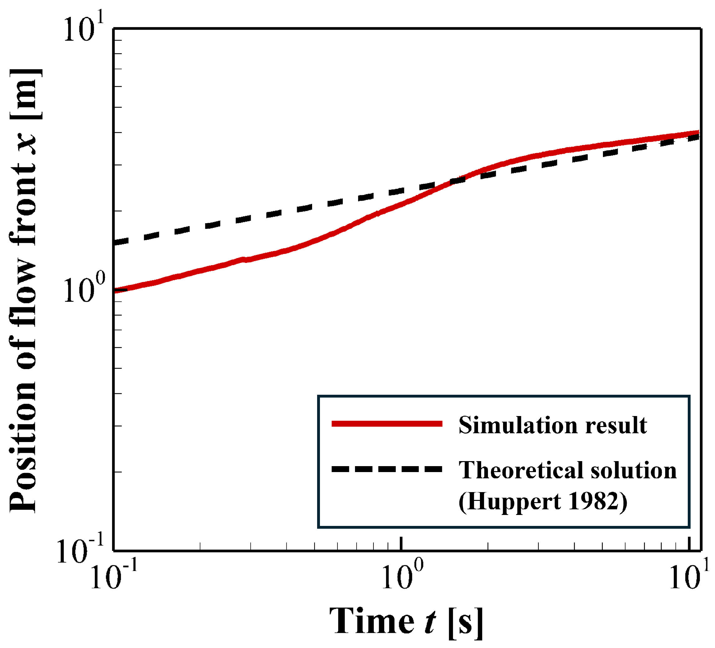
Figure 5.
Temporal evolution of the relative change of the compensated quantity . The vertical axis represents the relative change between consecutive time steps, defined as . The time interval between successive data points is .
Figure 5.
Temporal evolution of the relative change of the compensated quantity . The vertical axis represents the relative change between consecutive time steps, defined as . The time interval between successive data points is .
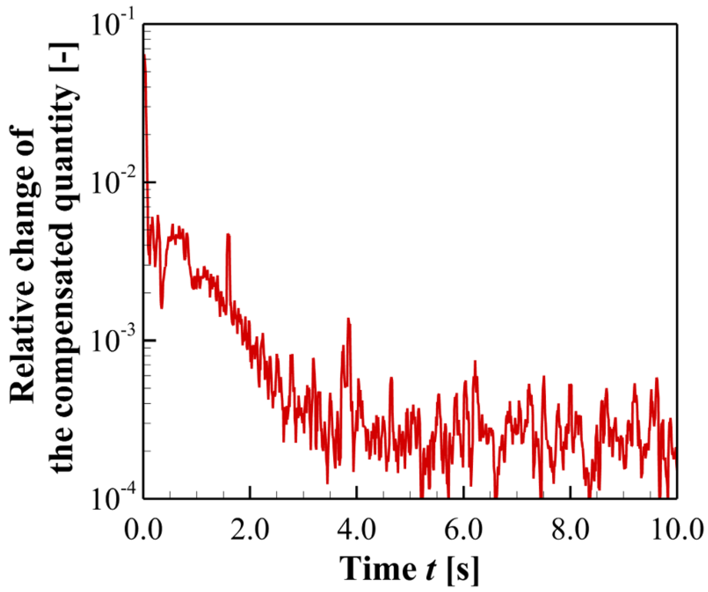
Figure 6.
Temporal evolution of the flow front position obtained from the numerical simulation for condition B. The solid line represents the simulation result. The thick dashed line indicates the theoretical stopping position predicted by Lyman [13]. The thin dashed lines represent the experimentally observed variability range of the stopping lengths, corresponding to 79–93% of the theoretical prediction.
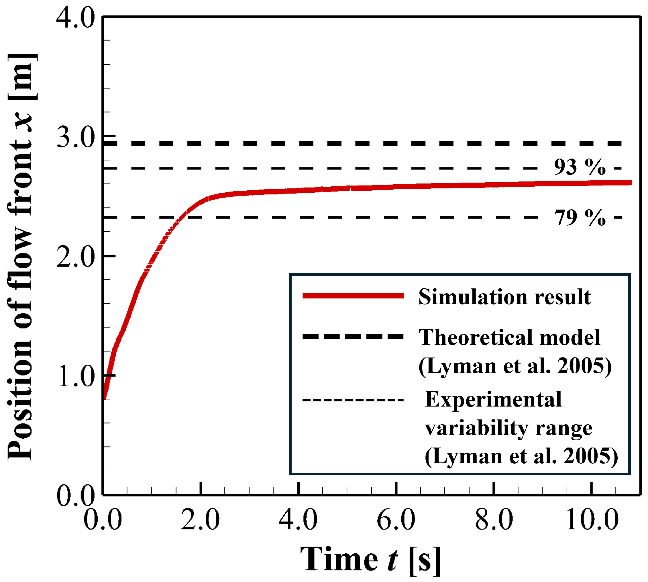
Figure 7.
Time evolution of the flow front position for each condition. The blue, green, orange, and red lines correspond to the conditions N, TN, B, and TB, respectively.
Figure 7.
Time evolution of the flow front position for each condition. The blue, green, orange, and red lines correspond to the conditions N, TN, B, and TB, respectively.
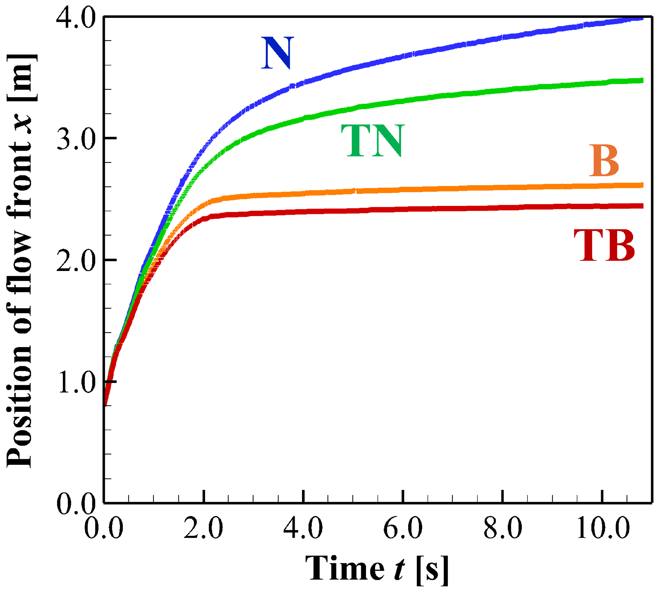
Figure 8.
x-directional velocity distributions when the flow front reaches at : (a) N, (b) TN, (c) B and (d) TB.
Figure 8.
x-directional velocity distributions when the flow front reaches at : (a) N, (b) TN, (c) B and (d) TB.
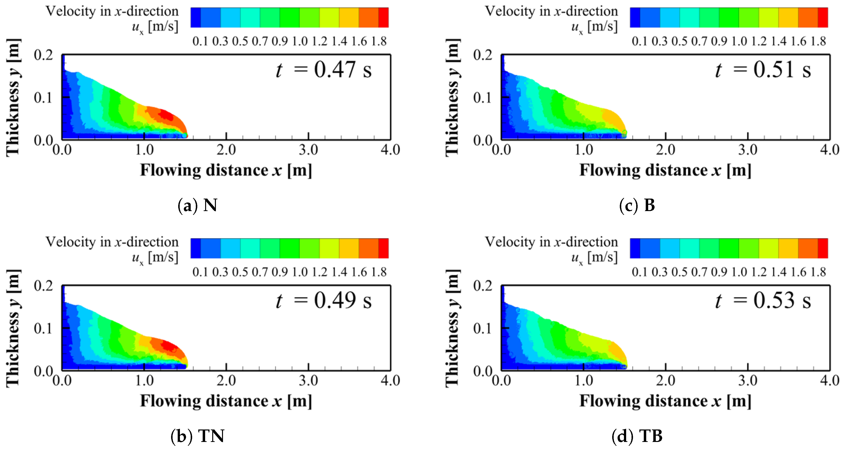
Figure 9.
x-directional velocity distributions when the flow front reaches at : (a) N, (b) TN, (c) B and (d) TB.
Figure 9.
x-directional velocity distributions when the flow front reaches at : (a) N, (b) TN, (c) B and (d) TB.
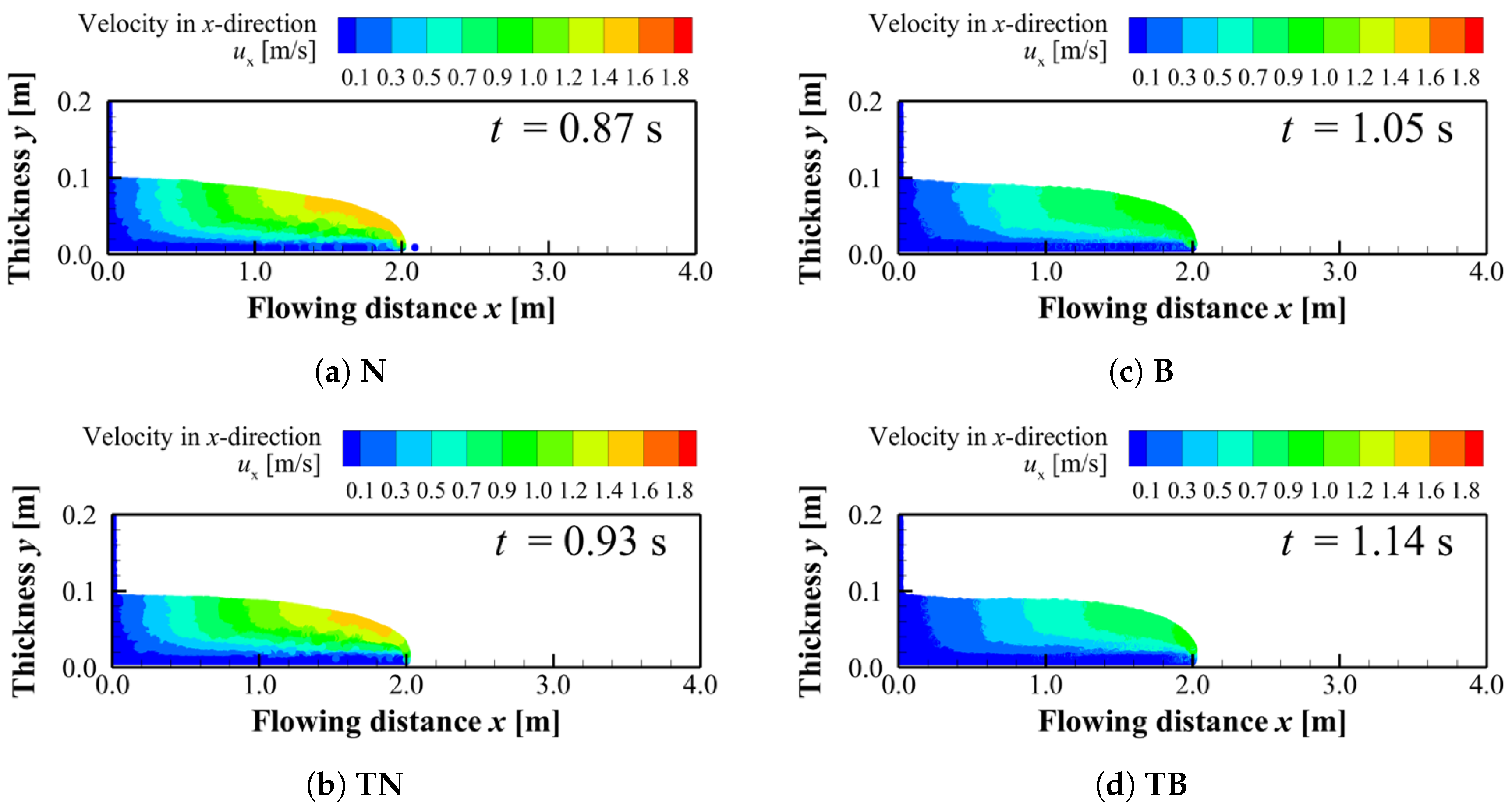
Figure 10.
x-directional velocity distribution when the flow front reaches at for N and TN and at for B and TB: (a) N, (b) TN (), (c) B and (d) TB ().
Figure 10.
x-directional velocity distribution when the flow front reaches at for N and TN and at for B and TB: (a) N, (b) TN (), (c) B and (d) TB ().
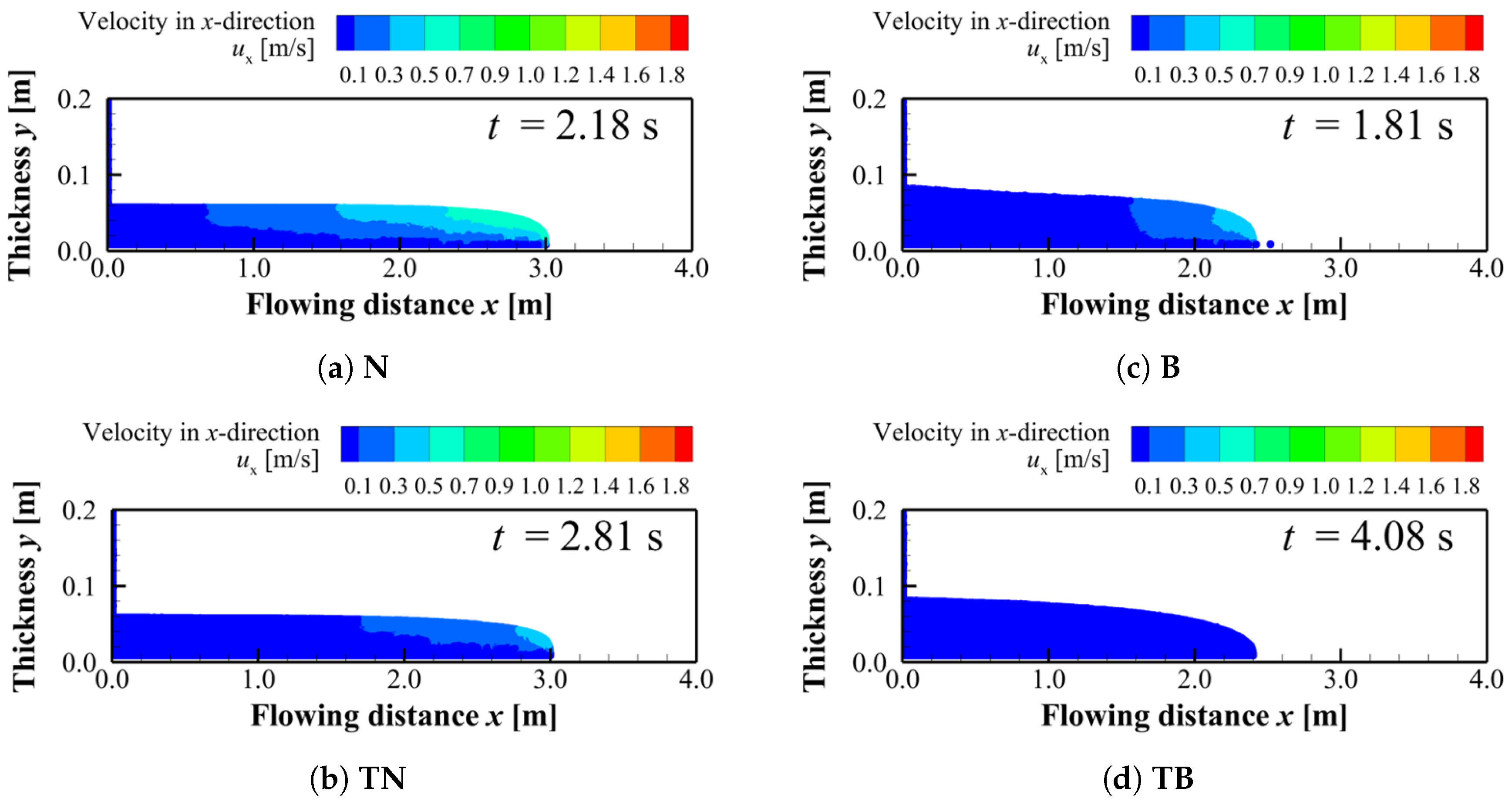
Figure 11.
x-directional velocity distribution at (when the flow front of condition N reaches the domain boundary): (a) N, (b) TN, (c) B and (d) TB.
Figure 11.
x-directional velocity distribution at (when the flow front of condition N reaches the domain boundary): (a) N, (b) TN, (c) B and (d) TB.
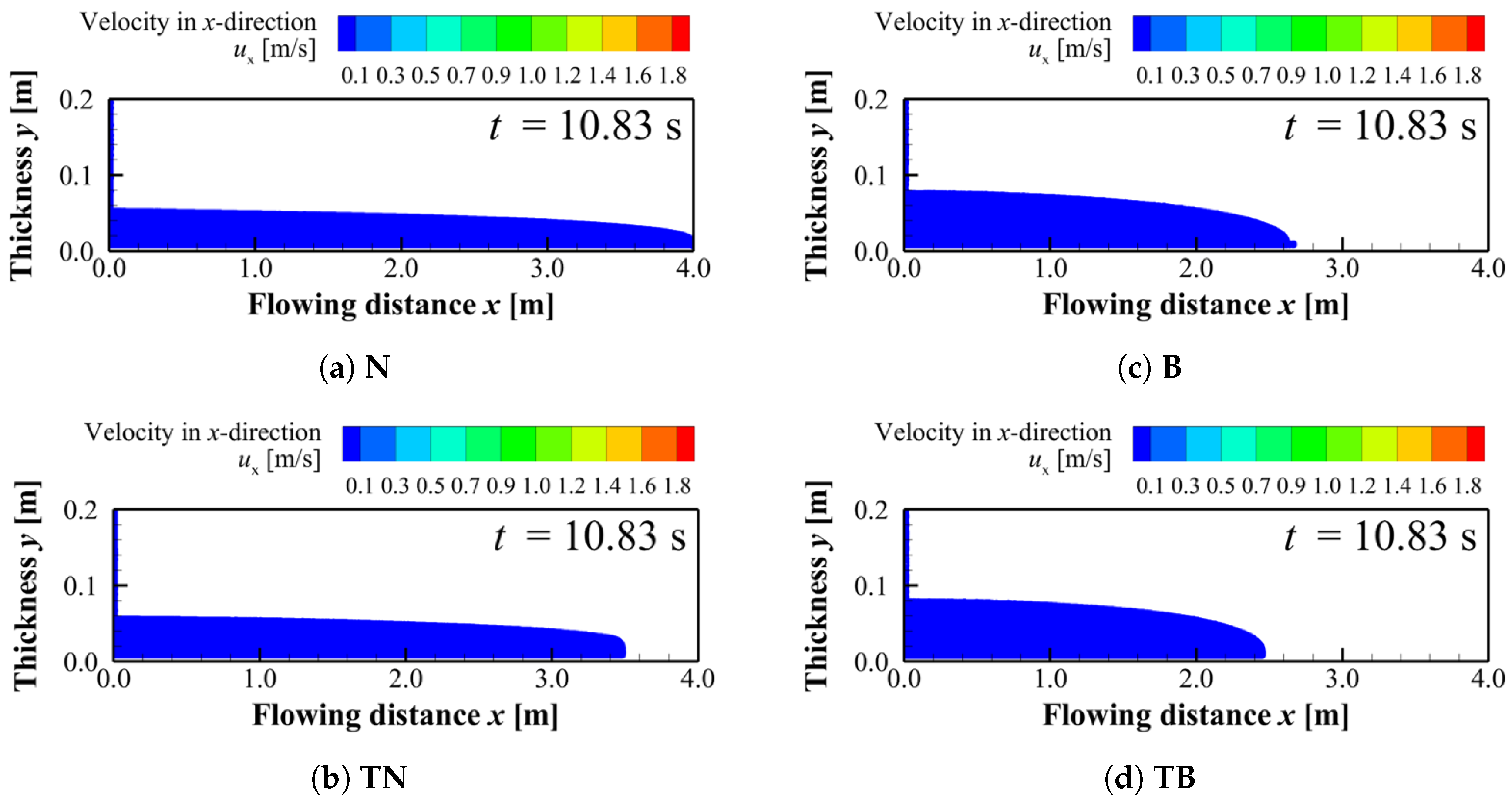
Figure 12.
Viscosity distributions for B and TB: (a) at the time B reaches at , (b) at the time B reaches at , (c) at the time TB reaches at and (d) at the time TB reaches at ,
Figure 12.
Viscosity distributions for B and TB: (a) at the time B reaches at , (b) at the time B reaches at , (c) at the time TB reaches at and (d) at the time TB reaches at ,
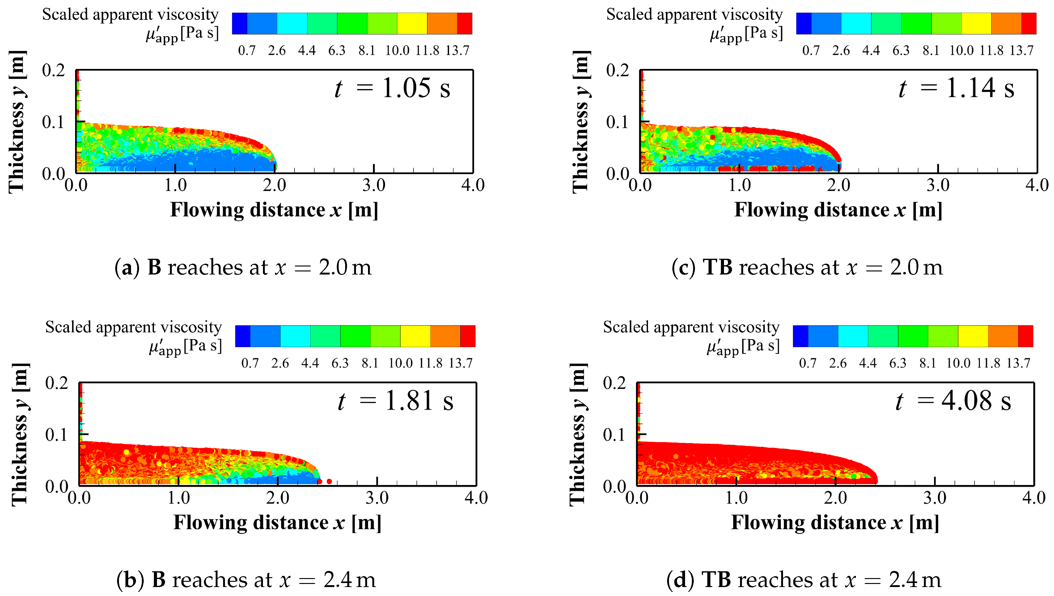
Figure 13.
Viscosity distributions at the time when the flow fronts reach : (a) N, (b) TN, (c) B (reprinted from Figure 12), (d) TB (reprinted from Figure 12).
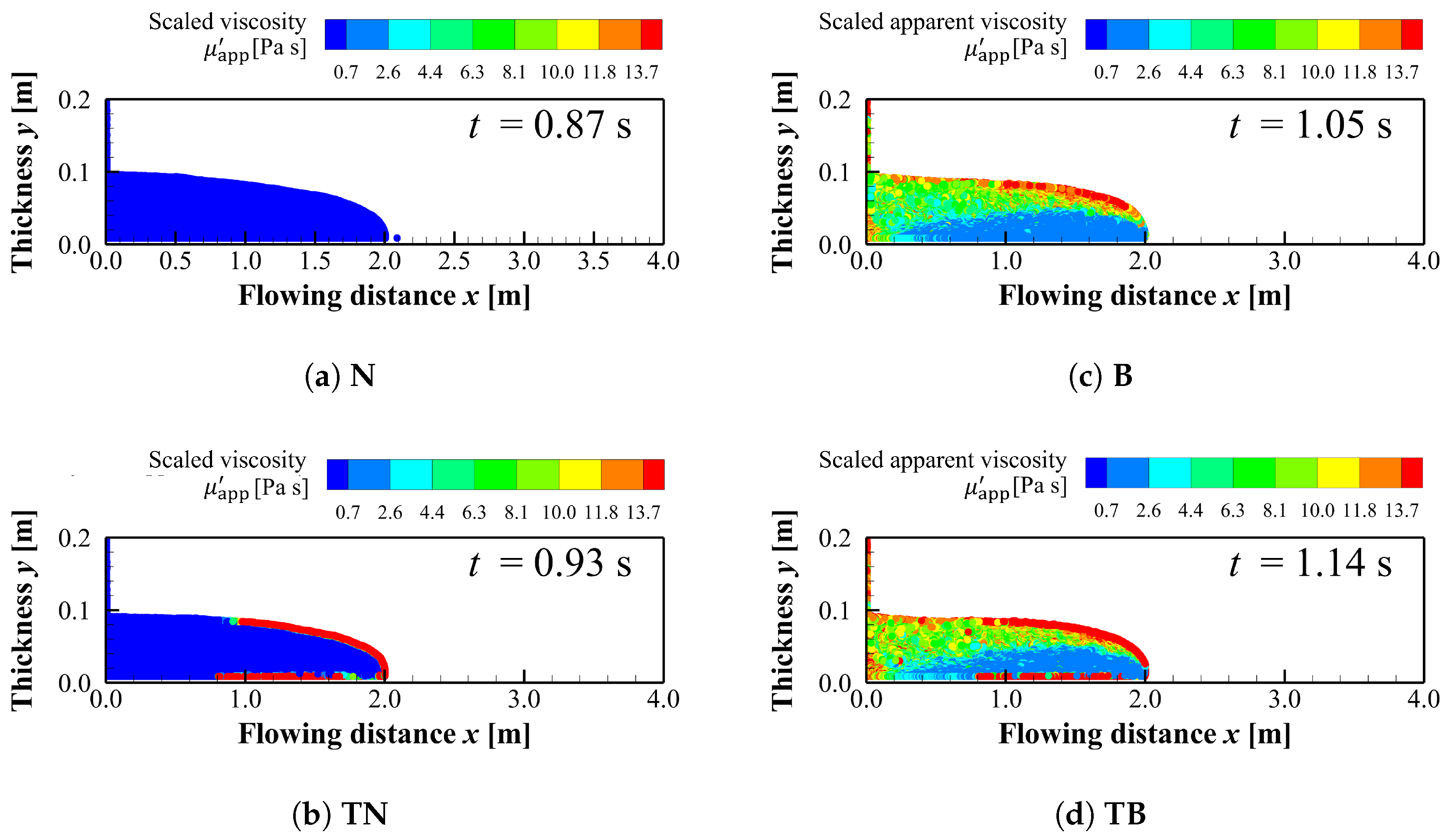
Figure 14.
Temperature distribution at the time when the flow fronts reach : (a) TN, (b) TB.
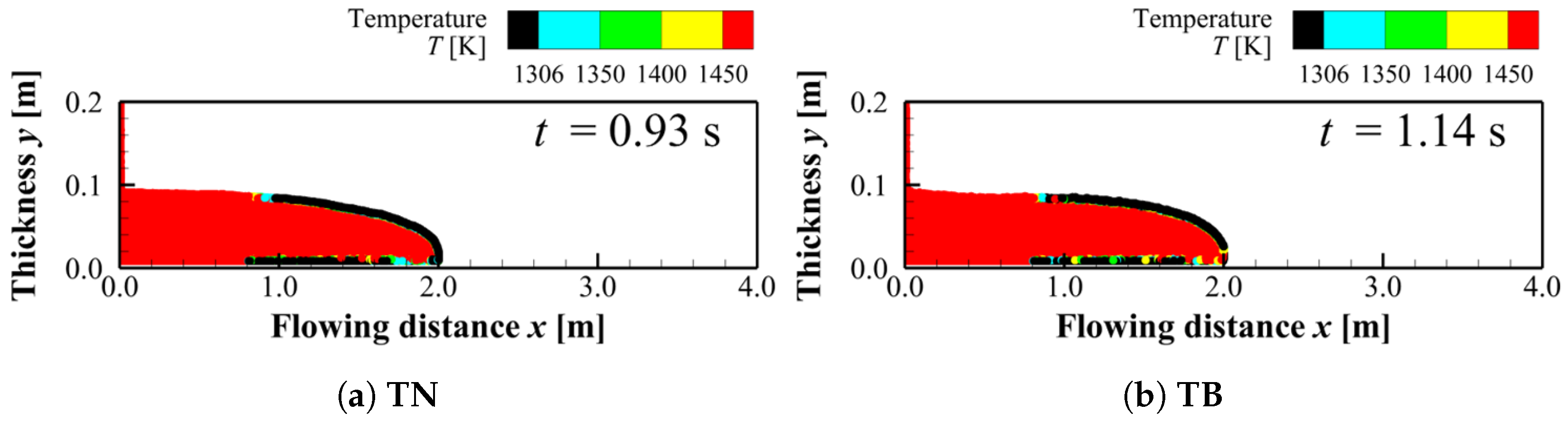

Table 1.
Computational conditions.
| Parameter | Value | Unit |
|---|---|---|
| Dimension number | 2 | - |
| Diameter of computational particle H | ||
| Time step | ||
| Gravitational acceleration g | ||
| Thermal conductivity of soil | ||
| Specific heat of soil | ||
| Density of soil | ||
| Temperature of air | 300 | |
| Thermal conductivity of air | ||
| Distance from surface particles to air |
Table 2.
Physical properties of basaltic lava.
| Property | Value | Unit |
|---|---|---|
| Density | ||
| Scaled apparent viscosity | – | |
| Fitting parameter for viscosity model | - | |
| Yield stress | ||
| Thermal conductivity | – | |
| Specific heat at constant pressure | – | |
| Emissivity | - |
Disclaimer/Publisher’s Note: The statements, opinions and data contained in all publications are solely those of the individual author(s) and contributor(s) and not of MDPI and/or the editor(s). MDPI and/or the editor(s) disclaim responsibility for any injury to people or property resulting from any ideas, methods, instructions or products referred to in the content. |
© 2026 by the authors. Licensee MDPI, Basel, Switzerland. This article is an open access article distributed under the terms and conditions of the Creative Commons Attribution (CC BY) license (http://creativecommons.org/licenses/by/4.0/).
Copyright: This open access article is published under a Creative Commons CC BY 4.0 license, which permit the free download, distribution, and reuse, provided that the author and preprint are cited in any reuse.


