Submitted:
01 January 2026
Posted:
05 January 2026
You are already at the latest version
Abstract
Generative diffusion models have emerged as a powerful class of models in machine learning, yet a unified theoretical understanding of their operation is still developing. This paper provides an integrated perspective on generative diffusion by connecting the information-theoretic, dynamical, and thermodynamic aspects. We demonstrate that the rate of conditional entropy production during generation (i.e. the generative bandwidth) is directly governed by the expected divergence of the score function's vector field. This divergence, in turn, is linked to the branching of trajectories and generative bifurcations, which we characterize as symmetry-breaking phase transitions in the energy landscape. Beyond ensemble averages, we demonstrate that symmetry-breaking decisions are revealed by peaks in the variance of pathwise conditional entropy, capturing heterogeneity in how individual trajectories resolve uncertainty. Together, these results establish generative diffusion as a process of controlled, noise-induced symmetry breaking, in which the score function acts as a dynamic nonlinear filter that regulates both the rate and variability of information flow from noise to data.
Keywords:
generative diffusion models
; stochastic thermodynamics
; information theory
; entropy production
; symmetry breaking
; phase transition
1. Introduction
Generative diffusion models have rapidly become one of the most successful frameworks for high-dimensional generative modeling. They were introduced in Sohl-Dickstein et al. [1] in analogy with stochastic thermodynamics. Several works elucidated the theoretical foundations of the method [2,3,4] and their practical implementation procedures [3,5]. Despite these efforts, a unified conceptual understanding of their behavior is still emerging. Several perspectives on information theory, stochastic thermodynamics, and the statistical physics of symmetry breaking have each shed light on different aspects of diffusion models, but their interrelations remain fragmented. The purpose of this perspective paper is to integrate these viewpoints into a single coherent theoretical picture.
Our central thesis is that generation in diffusion models proceeds through a sequence of noise-driven symmetry-breaking transitions. These transitions determine when and how the model commits to a specific generative outcome, structure the flow of information, regulate entropy production, and shape the geometry of trajectories in state space. We refer to this synthesis as the information thermodynamics of generative diffusion.
Information Theory and Entropy-Based Perspectives
A growing line of work has examined diffusion models from the standpoint of information theory, focusing especially on how information about the clean sample is progressively revealed as noise is removed. Recent works have proposed information-theoretic decompositions of diffusion dynamics [6,7] and have explored the role of conditional entropy in designing improved training and sampling schedules [8,9]. Furthermore, Franzese et al. [10] show how information-theoretic tools reveal the mechanisms by which latent abstractions guide generation. These approaches treat diffusion as a sequential information transfer process and highlight that the effectiveness of generation depends on how rapidly uncertainty about can be reduced. Central to these results is the observation that the conditional entropy rate is directly linked to geometric quantities such as the divergence of the score and the curvature of the log-density. This suggests that information flow is deeply connected to the underlying dynamical and geometric structure of the generative process.
Phase Transitions, Associative Memories, and Symmetry Breaking
Parallel developments in statistical physics have revealed that diffusion models exhibit noise-driven symmetry-breaking events, where the score field undergoes bifurcations and the generative trajectories split into distinct modes [11,12]. High-dimensional analyses have linked these transitions to mean-field phase transitions [13] and to dynamical behavior captured by stochastic localization [14,15,16,17]. These bifurcations correlate with sharp changes in the Hessian of the log-density, revealing a connection between symmetry breaking and information geometry. Similar mechanisms have been studied in hierarchical generative settings [18,19] and in analyses of memorization, mode formation, and semantic emergence [20,21,22,23]. Generative diffusion models have also been directly connected to modern Hopfield networks and other associative memory networks [24,25,26,27], where generalization has been associated with the emergence of spurious states [28]. Across these domains, the key unifying insight is that the Hessian (or score Jacobian) mediates both stability of generative trajectories and the structure of the data manifold.
Thermodynamics and the Role of Inferential Entropy
The connection between diffusion models and stochastic thermodynamics was first made explicit in Sohl-Dickstein et al. [1], motivating a thermodynamic view of generation. Furthermore, this connection was strengthened with a mathematical framework based on stochastic differential equations (SDEs) formulated in Song et al. [2], Rombach et al. [29] and is central to the modern understanding of diffusion models. However, the notion of entropy that is commonly used in stochastic thermodynamics [30,31] measures the irreversibility of the forward process. While such quantities yield elegant speed-accuracy tradeoffs [32], they characterize the evolution of the distribution of trajectories rather than the uncertainty relevant for generating a single sample. Instead, we argue that what matters during generation is the uncertainty about the clean sample .
For this reason, it is more natural to study the conditional entropy and, at the trajectory level, the pathwise conditional entropy , whose fluctuations capture the temporary multimodality experienced by individual generative paths. As in stochastic thermodynamics, such pathwise entropies can increase along single trajectories, even when the average conditional entropy decreases. We show that these fluctuations reveal symmetry-breaking events; the model becomes momentarily undecided among competing hypotheses for , leading to spikes in conditional entropy variance and amplified sensitivity to noise.
Our Perspective
We unify these threads by showing that information flow, symmetry breaking, and dynamical instability are different manifestations of the same underlying mechanism governing diffusion models. In particular, we show that:
- Entropy as a detector of symmetry breaking: Symmetry-breaking transitions are accompanied by pronounced changes in ensemble-level information measures. In particular, the conditional entropy rate exhibits sharp peaks around bifurcation points, reflecting an increased sensitivity of the generative process to noise. These peaks provide direct information-theoretic signatures of symmetry-breaking transitions.
- Noise-driven decisions: These information-theoretic signatures arise when the score field becomes weak along a low-curvature direction, temporarily losing its ability to suppress stochastic fluctuations. In such regimes, noise plays an active role in selecting which generative branch the trajectory follows, effectively making the generative decision.
- Path divergence via Lyapunov instability: The same loss of curvature is reflected in the Jacobian of the score, whose spectrum develops positive eigenvalues along the unstable directions. As a result, nearby generative trajectories diverge exponentially, leading to macroscopic separation between paths that correspond to different generative outcomes.
- Non-monotonic pathwise entropy: At the level of individual trajectories, this divergence manifests as heterogeneous resolution of uncertainty about . Consequently, the pathwise conditional entropy need not evolve monotonically along single paths and may transiently increase, reflecting temporary ambiguity during the symmetry-breaking decision process. This results in the variance of pathwise conditional entropies peaking.
Together, these results establish a conceptual framework in which entropy production, posterior geometry, and dynamical stability are unified through the lens of noise-driven symmetry breaking. This perspective clarifies the mechanisms by which diffusion models transform noise into structured data and highlights the central role of symmetry in shaping generative dynamics.
2. Information Theory
We start by presenting an introduction to the information theory of sequential generative modeling, which will open the door to the analysis of generative diffusion.
Consider a game of Twenty Questions where an interrogator player may ask twenty binary questions concerning a set to an "oracle" player in order to gradually reveal the identity of a predetermined element in a finite set with elements. We denote the size of the possible set after questions as . The answer to the j-th question then divides the set into two possible subsets with sizes and . Assuming a fixed set of questions, the expected uncertainty experienced by the player after the j-th question can be quantified by the conditional entropy:
where is sampled uniformly from . Under these conditions, the expected entropy reduction associated to a given question is given by
where we left the dependence on the set of answers implicit to unclutter the notation. It is easy to see that the maximum bit rate is 1, which is achieved when . Assuming that 20 questions are enough to fully identify the value of , we can encode each in the string of binary values , which makes clear that the question answering process consists of gradually filling in this string. Using the language of generative diffusion, we can re-frame this process in terms of a ’forward’ process, where the string corresponding to an element of is sampled in advance and then transmitted to the j-th ’time point’ through the following non-injective forward process
which deterministically suppresses information by masking the values of the string. The solution of a Twenty Question game can then be seen as inverting this ’forward process’. Note that the forward process leads to a sequence of monotonically non-decreasing marginal conditional entropies , which is a fundamental feature of a forward process in diffusion models that captures the fact that information is lost by the forward transformation.
Now consider the case where a lazy oracle forgot to select a word in advance and decides instead to answer the questions at random under the probability determined by the sizes and , which we assume to be fixed given the questions. Strikingly, this reformulation does not make any observable difference from the point of view of the interrogator as each (randomly sampled) answer equally reduces the space of possible words and it results in the same entropy reduction, until a final guess can be offered. Therefore, the game of Twenty Questions with a random oracle can be interpreted as a sequential generative process where the state at ’time’ j is given by a binary string with Markov transition probabilities
The conditional entropy rate determines how much information is transferred from ’time’ j to the final generation.
As we shall see, the reverse diffusion process can be seen as analogous to this ’generative game’ with the score function playing the part of the interrogator and the noise playing the role of the oracle. Like in the interrogator in the generative Twenty Questions game, the score function can reduce the information transfer by tilting the probabilities of the stochastic increments out of uniformity, which reduces the impact of the noise. This phenomenon is related to the divergence of the vector field induced by the score function, which causes amplification of small perturbations during the generative dynamics. We will also see that the phenomenon is connected to the branching of paths of fixed-points of the score and consequently to the phenomenon of generative phase transitions and spontaneous symmetry breaking [11].
2.1. Score-Matching Generative Diffusion Models
The sequential generation example outlined above is analogous to the masked diffusion models [33,34]. On the other hand, score-matching generative diffusion models are continuous-time sequential generative models where the forward process is given by a diffusion process such as
which is initialized with the data source . Generation in score-matching diffusion consists of integrating the ’reverse equation’ [2]:
where, for notational simplicity, we restrict our attention to the forward process given in Eq. 5. Note that Eq. 6 must be integrated backward with initial condition determined by the stationary distribution of the forward process.
The fundamental mathematical object that determines the reverse dynamics is the score function, which in this case can be expressed as where is the total variance of the noise at time t and the expectation is taken with respect of the conditional distribution . This expression can be further simplified by noticing that :
where is a standard normal vector. In other words, the score is the negative of the average (rescaled) noise and it therefore provides the optimal (infinitesimal) denoising direction.
In dynamical term, the score function determines the vector field (i.e. the drift) that guides the generative paths towards the distribution of the data.
In practice, a normalized score network should be trained to minimize the rescaled score-matching loss:
This loss function cannot be computed directly because the true score is not available. However, Eq. 8 can be re-written using Eq. 7 and expanding the square:
Note that the second term is constant in , which means that the gradient solely depends on the denoising loss:
The constant term
is of high importance for our current purposes. It quantifies the loss of the denoiser obtained from the score function. This is therefore the unavoidable part of the denoising error that is still present given a perfectly trained network. With a few manipulations, it is possible to show that this term is in fact equal to the variance of the posterior denoising distribution:
which allows us to interpret this term as a measure of uncertainty at time t on the final outcome of the generative trajectory.
3. Generative Information Transfer in Score Matching Diffusion
To characterize the generative information transfer we need to compute the conditional entropy rate , which is the analogous of the discrete entropy reduction we gave in Eq. 2. The conditional entropy is defined as
To find the entropy rate, we can take the temporal derivative of Eq. 13 and use the Fokker-Planck equation, which in our case is just the heat equation:
Using integration by parts, this results in
where D is the dimensionality of the ambient space. From this formula, we can see that the maximal bandwidth is reached when the Euclidean norm of the score function is minimized.
3.1. Score Norm and Posterior Concentration
To gain some insight on the significance of the square norm and the expression for the conditional entropy we will consider the following case. We assume a discrete data distribution with empirical mean equal to zero.
At time t, the marginal density is given by a Gaussian smoothing of the data,
where denotes an isotropic Gaussian with variance . The posterior distribution over datapoints is
The score function can then be written as the posterior average
We now assume that the data vectors satisfy
i.e. datapoints are approximately orthogonal and lie at a common distance R from the mean. Under this assumption, the squared norm of the posterior mean simplifies to
Taking expectations with respect to , we obtain
The first term captures the data-dependent structure of the score and, using Eq. (20), can be written as
The quantity measures the concentration of the posterior over datapoints. It satisfies , interpolating between a fully diffuse posterior and complete concentration on a single datapoint.
The remaining two terms in Eq. (21) can be estimated explicitly under the forward model , where is independent of y. We have
where D denotes the ambient dimensionality.
The second term coincides with the expected squared norm of the score of the forward Gaussian kernel and therefore represents a data-independent baseline contribution. The first term encodes the deviation from pure diffusion induced by the structure of the dataset and depends solely on the posterior distribution over datapoints.
Using the bound , we obtain the inequality
As a consequence, the expected squared norm of the score is always bounded above by the forward kernel contribution, ensuring that the marginal entropy remains a monotonically increasing function of time.
Further insight can be gained by rewriting the purity term as
This expression makes explicit that the deviation from the diffusion baseline is controlled by the overlap of the forward kernels. If, at time t, the datapoints have effectively merged into m indistinguishable groups (with identical posteriors), the purity evaluates to , yielding
Therefore, increasing mixing among datapoints (smaller m) makes the data-dependent term more negative, reducing the expected score norm and increasing the conditional entropy rate.
This result allows us to interpret the magnitude of the score vector as a quantitative estimate of uncertainty in the denoising process: when multiple datapoints are compatible with the noisy state , posterior averaging suppresses the score, leading to enhanced entropy production (equation 15). As we shall see in the rest of the paper, we can associate peaks in the entropy rates with symmetry-breaking bifurcations that correspond to noise-induced ’choices’ between possible data points.
3.2. Conditional Entropy Production as Optimal Error
The conditional entropy rate quantifies the instantaneous generative information transfer at any given moment in time. It can be shown (see [8]) that this quantity is closely connected to the optimal denoising squared error, which is the variance of the denoising distribution:
Intuitively, this means that the information rate is directly related to the denoising uncertainty at a given time.
Using this relation, we can now re-express the denoising score matching formula in Eq. 9 in terms of the conditional entropy rate:
which implies that the entropy rate can be estimated from the training loss if we assume that the network is well-trained.
3.3. Generative Bandwidth
It is insightful to investigate under what circumstances the score-matching diffusion model can achieve the maximum possible generative bandwidth. From equation 15, it is clear that this happens when , which in turn is obtained if the score vanishes almost everywhere.
To realize this situation, we can consider a data distribution to be a centered multivariate normal with variance . In this case, the score function is just:
which vanishes everywhere for , giving a maximum entropy rate:
This corresponds to a setting where the particles are free to diffuse since every possible generation is equally likely. From this, we can conclude that the score function has the negative role of suppressing fluctuations along ’unwanted directions’ to preserve the statistics of the data and that peaks in the information transfer comes from periods where noise fluctuations are not suppressed. Note that the maximum bandwidth scales with the dimensionality D.
Now consider the case where the distribution of the data is a centered Gaussian in a -dimensional subspace with . In this case, the expected norm of the score decomposes as follows
which leads to the entropy rate
In this case, the score function suppresses entropy reduction in the subspace orthogonal to the data and therefore acts as a linear analog filter. Note that the entropy rate is zero when is equal to zero since all the distribution is in this case collapsed into a single point and no ’decision’ needs to be made.
4. Statistical Physics, Order Parameters and Phase Transitions
In this section, we will connect the information theoretical concepts we outlined above with concepts from statistical physics such as order parameters, phase transitions and spontaneous symmetry breaking. We will start by studying the paths of fixed-points of the score function and use them to track ’generative decisions’ (i.e. bifurcations) along the denoising trajectories. As we will see, the stability of these fixed-points paths is regulated by the Jacobian of the score and it is deeply connected with the conditional entropy production.
4.1. Branching Paths of Fixed-Points and Spontaneous Symmetry Breaking
The fixed-points of the score function are defined by the equation:
We denote the set of fixed-points at time t as . The solutions of this fixed-point equation can be organized in a set of piecewise continuous paths . To remove ambiguities, we assume that, if is discontinuous at , then the one-sided limit exists and is equal to . We know that for all paths since the zero vector is the only fixed-point of the score of the asymptotic Gaussian distribution. Any two paths and can be proven to overlap for a finite range of time, meaning that if (this follows from the results in [35,36,37] on the number of modes of mixture of normal distributions). We refer to as the branching time of the two paths. The branching time of two paths of fixed points can roughly be interpreted as a decision time in the generative process, where the sample will be ’pushed’ by the noise in either one or the other path during the reverse dynamics. It is therefore insightful to study the behavior of the paths at the branching times. In general, this can happen if there is a discontinuous jump in a path . Perhaps more interestingly, two paths can also branch continuously at a finite time. This can be studied by analyzing the Jacobian matrix of the score function:
We call a path point stable at time t if is negative-definite. We say that the path is stable if this is true for all except for a countable set of time points where the Jacobian is negative semi-definite. Now consider two stable paths and that branch continuously at time . Given the asymptotic separation vector
it can be shown that in a finite interval and that
which implies that the second directional derivative of along vanishes at the branching point.
Consider now a generative diffusion with an initial distribution given as
with K distinct data-points . In this case, there are exactly K distinct stable fixed-point paths , with . Again, any two paths branch at a finite time . For a given t, we can partition the set of data-points in equivalence classes, where two data-points and share the same class if their associated path coincide at t. Importantly. Each equivalence class corresponds to an individual fixed-point, which allows us to associate each fixed-point to a sub-set of data-points that are, using colorful language, fused together. More precisely, we can express the fixed-points as weighted averages of data-points obtained by solving the self-consistency equation:
where
Note that this average has non-zero weight on all data points, which is why we cannot find the location of the fixed-point solely based on its equivalence class. However, usually the weights corresponding to data-points in the equivalence class will be substantially larger than the other weights and will therefore dominate the average. In summary, we can interpret the set of fixed-points as a decision tree where each branching point roughly coincides with a split between two sets of data points.
An example of spontaneous symmetry breaking happens when the generative path needs to ’decide’ between two isolated data-points. Consider again the mixture of delta case and two neighboring data-points and . If the distance between the center of mass of these two points and the nearest external data-point is much larger than , there will be a fixed point approximately located along the line segment connecting the two points. In these conditions, we can consider the fixed-point equation restricted to the projections on :
where encapsulates the interference due to all other data-points, which we, in this example, we assume to be small relative to the norm of the separation vector:
If we approximate the interference function with constant using a zero-th order Taylor expansion, Eq. 40 becomes the self-consistency equation of a Curie-Weiss model of magnetism, with temperature and external magnetic field . The solutions of this equation can be visualized as intersection points between a straight line and a hyperbolic tangent (see [12] and [11] for a detail analysis). When is finite, the system transitions discontinuously from one to two fixed-points, which corresponds to a first-order phase transition in the magnetic system. However, the size of the discontinuity vanishes when , when there is an exact symmetry between the two data-points (see Figure 1). This gives rise to a so called critical phase transition, where a single fixed-point at continuously splits into two paths and with for . The loss of stability of the fixed-point at the origin corresponds to the vanishing of the quadratic well around the point:
where, in this case, for . The analysis we just carried out involves the breaking of the permutation symmetry between two isolated data-points. On the other hand, if the symmetry is broken along all directions like in the case where the data manifold is a sphere centered at , Eq. 41 implies that
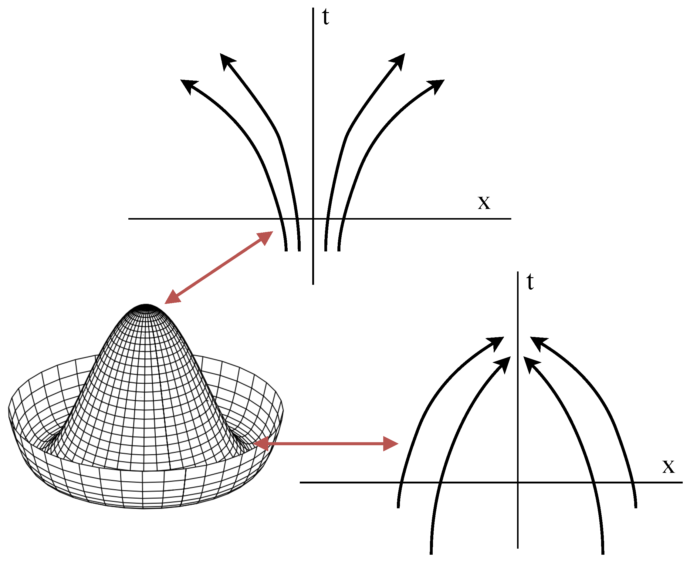
Therefore, the change in stability condition can be reformulated as the local vanishing (or suppression in a less symmetric case) of the divergence of the vector field that drives the generative dynamics. The transition from the super-critical () and the sub-critical ( phases then corresponds to a sign change in the divergence of the vector field (i,e, the score) in the spherically-symmetric case, or a sign change of the divergence restricted to a sub-space in the general case, with the sub-critical regime being characterized by positive eigenvalues of the Jacobi matrix that lead to divergent local trajectories (see Figure 2).
5. Dynamics of the Generative Trajectories
Around a point , the local behavior of the generative trajectories under the deterministic ODE flow dynamics can be characterized by its Lyapunov exponent, which quantifies the separation rate of infinitesimally close trajectories. In particular, the minimal local exponent for a perturbation along a unit vector , which in the reverse dynamics can be defined as
where denotes a deterministic generative trajectory with the perturbed initial condition. Note that in reality cannot tend to infinity in the generative dynamics since time is only defined up to 0. However, we will still consider this limit since we are only interested in the local asymptotic behavior of the linearized dynamics around a bifurcation point. Under the reverse dynamics, when the Lyapunov exponent along is negative, infinitesimal perturbations are amplified exponentially (at least locally) by the generative dynamics.
We can use the notion of minimal local Lyapunov exponent to formalize the phenomenon of local divergence of trajectories after a spontaneous symmetry-breaking event at . To study the local sub-critical behavior, we consider the linearization of the dynamics around the unstable fixed point for and :
where is the smallest of the eigenvalue of the Jacobi matrix whose eigenvectors overlap with . In the immediate sub-critical phase of a symmetry breaking phase transition, we know that there is a non-empty sub-space spanned by the eigenvector of the Jacobian corresponding to negative eigenvalues. Therefore, perturbations along this unstable eigen-space will be exponentially amplified by the generative dynamics. In the stochastic case, this can be seen as a critical ’macroscopic amplification’ of the infinitesimal noise input, where the noise breaks the symmetry of the generative model. In the deterministic dynamics, the symmetry is instead broken by the amplification of small differences between the generative trajectories.
In general, we will refer to the spectrum of Jacobian eigenvalues as the local Lyapunov spectrum. As we shall see, this spectrum can be directly related to the conditional entropy production.
5.1. The Global Perspective on Generative Bifurcations
In the previous sections, we characterized the generative dynamics of diffusion models by studying the associated paths of fixed-points in term of their stability and bifurcations, which led us to establish formal connections with the statistical physics of phase transitions and symmetry breaking. However, in high dimension, small volumes around a fixed-point have vanishingly low probability of being visited. In fact, due to the dispersive effect of the noise, the generative trajectories are concentrated on fixed-variance shells around the fixed points. More formally, these set of "typical" points form tubular neighborhoods of the set of fixed-points (see Figure 1). It is therefore unclear how a bifurcation in a path of fixed-points affects the behavior of the generative trajectories, since the analysis we presented in the previous sections was purely local.
To gain insight into the global behavior of the typical generative trajectories, we can study the expected divergence of the vector field at time t
If is negative, the separation between the generative trajectories will, on average, be contracted by the generative dynamics. The simplest example of this contractive behavior can be studied by considering a data distribution with a single point: . In this case, all trajectories converge to for , and we have
where D is the dimensionality of the space. In the reverse dynamics, the negative sign implies that the forward process produces a stable dynamics where the particles ’fall’ towards the data points.
In the general case, this quantity can be identified with the "trivial component" of the expected divergence since it does not depend on the data but only on the forward process. In the general case, it can be expressed as
We can therefore study the purely data-dependent part of the expected divergence by subtracting this "trivial component":
Intuitively, encodes the separation of the typical trajectories in the reverse process due to bifurcations in the generative process, which mirrors the local analysis we carried out in the previous sections at the level of the fixed-points.
Using integration by parts, it is straightforward to connect the expected divergence with the conditional entropy rate
Therefore, the expected data-dependent divergence of the generative trajectories directly determines the conditional entropy rate. From this identity, we can immediately deduce that is non-negative valued and consequently that .
We can also show that the marginal entropy is produced by the expected divergence
which implies that since the marginal entropy is a monotonically increasing function of t under our forward process. This reflects the fact that the forward process always lead to a dispersion of the trajectories, regardless to the nature of the initial distribution. From this, we can conclude that the maximum bandwidth is achieved when
This gives us a clear connection between the local vanishing of the Jacobian in spontaneous symmetry breaking (Eq. 42) with the expected vanishing that corresponds to saturation of the generative bandwidth.
5.2. Information Geometry
The derivation in the previous sub-section suggests a deep connection between the information production and the geometry of the data manifold. We can further analyze this connection by using concepts from information geometry [38]. The key connection is that conditional entropy rate is in fact just the expected value of the trace of the Fisher information matrix, which can be defined as follows:
This quantity quantifies the sensitivity of the posterior distribution to changes in and can be interpreted as a natural metric tensor on the variable . Using Bayes theorem and our simplified forward process, the expression can be rewritten as
Geometric information such as the manifold dimensionality is encoded in the spectrum of this matrix [22,39,40,41]. The Fisher information metric provides information on the (local) manifold structure of the data as seen through the lenses of the noisy state . This is easy to see in the case where the data is Gaussian with covariance matrix , which gives the formula
When is supported on a manifold, the (degenerate) eigenvalue corresponding to the orthogonal complement is equal to zero. On the other hand, in the flat limit, the tangent eigenvalues become equal to . This implies that the dimensionality of the manifold is given by the dimensionality of the eigenspace corresponding to the eigenvalue . In the general case, the eigen-decomposition of characterizes the local tangent structure of the manifold [40,41].
We can now use these expressions to cast light on the geometry of entropy production. The conditional entropy rate is directly related to the trace of the Fisher information matrix:
which reduces to Eq. 34 in the linear manifold case we just considered. From this perspective, it is clear that the reduction in bandwidth is the result of the suppression of the eigenvalues of . This can also be seen in the general case by re-expressing the entropy rate in terms of the expected eigenvalues of the Jacobi matrix:
This equation shows that the entropy production is directly regulated by the spectrum of expected local Lyapunov exponents, as studied in our local analysis.
We can better understand this formula by rewriting it as follows:
From this, we can see that conditional entropy production in an eigenspace is fully suppressed when , which is the eigenvalue of the Jacobian of the conditional score under the isotropic forward process.
6. A Stochastic Thermodynamic Perspective
A central question in generative diffusion is how uncertainty about the clean sample is resolved as the model evolves from the noisy state toward the data manifold. As argued throughout this paper, the appropriate notion of inferential uncertainty is the previously discussed conditional entropy and, more fundamentally, its pathwise realization. The study of pathwise entropy is naturally motivated by ideas from stochastic thermodynamics. However, we believe that the commonly used entropy in stochastic thermodynamics [30,31] is not the correct quantity for understanding generative dynamics. It measures the irreversibility of the forward diffusion, not the uncertainty relevant to generating a single outcome.
For a given point on the trajectory , we define its path-dependent conditional entropy as
This quantity measures the uncertainty experienced along a single generative path. Its expectation is the usual conditional entropy,
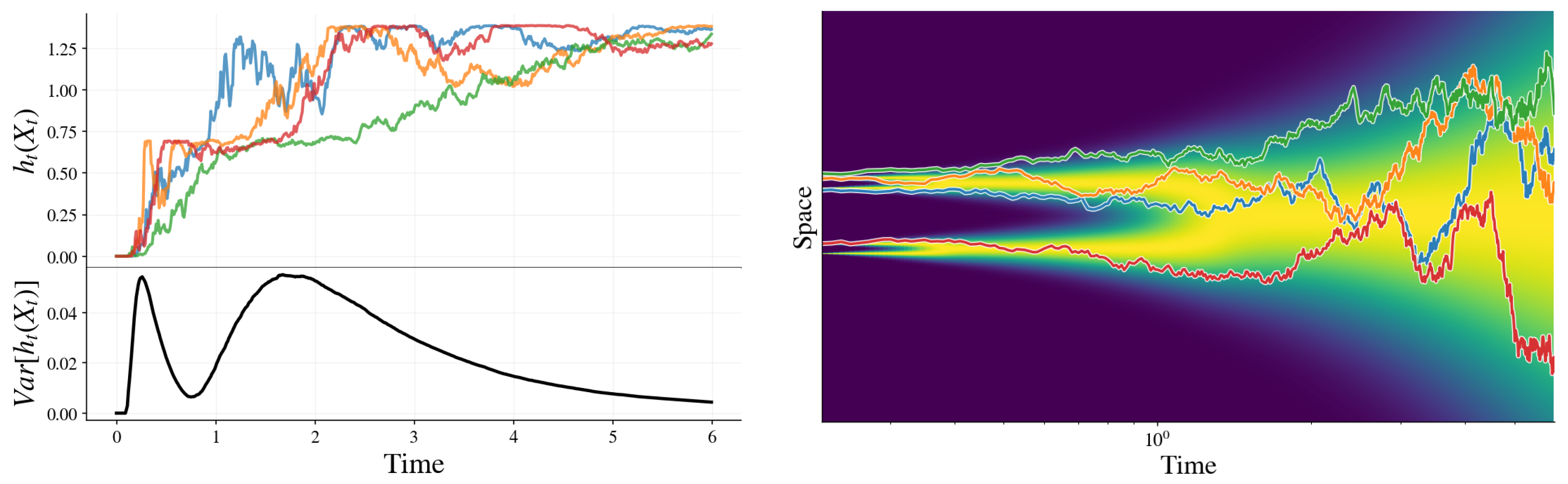
but its fluctuations encode a structure that is invisible to marginal entropies. In particular, as illustrated in Figure 3, the pathwise conditional entropy can locally increase along individual generative trajectories even as the mean conditional entropy decreases, a behavior reminiscent of entropy fluctuations in stochastic thermodynamics. Such effects do not arise in autoregressive models, where each generation step reduces uncertainty about the final sequence by revealing one token, since . Whether these entropy fluctuations in diffusion-based generation have any practical advantage, however, remains an open question.
To expose this dynamical heterogeneity, we consider the variance of the pathwise conditional entropy,
Figure 3.
An example of conditional entropies and corresponding paths for a dataset of four data points.
Figure 3.
An example of conditional entropies and corresponding paths for a dataset of four data points.
6.1. Variance of Pathwise Conditional Entropy as a Signature of Symmetry Breaking
We find that the variance captures both symmetry-breaking transitions (see Figure 3). To gain a better understanding, we explore the general behavior of the variance and demonstrate a connection with the speciation time [20].
Two limits are immediate. At very early times, the noise scale is negligible compared to the curvature of the data manifold. The posterior is effectively confined to the local tangent plane, behaving as an isotropic Gaussian whose shape is determined solely by the intrinsic dimension (we assume that the dimension is uniform across the manifold). Because the entropy of this Gaussian depends on k and t but is insensitive to the specific location on the manifold,
At very late times, the diffusion has effectively mixed the data distribution: carries little discriminative information about the origin and the posterior becomes approximately independent of , again implying
Thus, nontrivial variance can only arise in an intermediate regime where different trajectories resolve uncertainty in different ways.
Furthermore, near a bifurcation/decision time , the ensemble contains a substantial fraction of trajectories that are already decisively committed to a branch and a substantial fraction that remain ambiguous. In this regime, becomes broadly distributed (some paths yield low entropy, others high entropy), and is therefore maximized.
6.1.1. Connection with the Speciation Time
As already hinted, the variance of the pathwise conditional entropy can be used to locate the speciation time for Gaussian-mixture data in the sense of Biroli et al. [20]. We provide a short argument for why peaks at the speciation crossover by using a two-region picture of Biroli et al. [20]: points where the class is effectively determined versus maximally mixed. A fully rigorous derivation is possible, but we focus on the essential mechanism and keep the argument streamlined to make the discussion clear and self-contained.
Recall that Biroli et al. [20] define the speciation time as the crossover at which (viewed in the forward noising process) the injected noise blurs the principal “class” direction so that class identity becomes hard to infer; equivalently, by time-reversal, it is the time in the backward process at which trajectories start to commit to one of the classes.
We start by noticing that a single Gaussian has . If and the forward kernel is Gaussian, then is Gaussian with covariance independent of , so is constant and the variance vanish.
Let with latent index , and let be the (Gaussian) forward noising kernel. Define the pathwise conditional entropy
Now, assume that the mixture is well-separated. For each fixed t, the posterior admits the standard separated-mixture approximation
where is Gaussian, hence for all z. Using the entropy decomposition for (nearly) disjoint mixtures then yields
so the fluctuations of are governed by those of the discrete uncertainty .
Let be the posterior class weights and fix a small . For each t define the two subsets
and write and . The dynamical-regimes setting precisely corresponds to the statement that, for the mixture-of-Gaussians class considered in Biroli et al. [20], the regions and carry the most mass for times outside a narrow window around the speciation time, i.e. or except near .
On , the posterior is nearly one-hot, while on , the posterior is close to . Hence, neglecting the small boundary region , the random variable is approximately:
As a consequence, the variance admits the sharp lower/upper control
where we used that, when is negligible, and the variance of a two-point mixture is the product of the two masses times the squared gap. Equation (63) makes the mechanism transparent: the variance is small when essentially all points are class-diagnostic () or essentially all points are well-mixed (), and it is largest when the population splits nontrivially.
To connect this directly to the dynamical-regimes diagnostics, note that the cloning “same-class” probability can be written as
Pre-speciation, is almost one-hot for typical , so and thus , implying . Post-speciation (well-mixed), for typical , so and thus , again implying . Since varies continuously with t (it is an expectation of a bounded, smooth functional of the time-marginal under the Gaussian kernel), it must interpolate continuously between these limiting values; correspondingly, the mass must continuously move from to . Therefore the product necessarily becomes in the crossover window, and by (63) must develop a peak there. Under the dynamical-regimes picture where the transition in sharpens with dimension/separation, this peak concentrates around the speciation time .
For more general distributions (e.g. strongly non-Gaussian components), can also exhibit an additional early-time peak associated with rapid local “Gaussianization” of under the forward kernel. This peak is absent for the ideal Gaussian case and is suppressed when each component is close to Gaussian.
7. Discussion & Conclusions
This paper has presented a unified framework that connects the dynamics, information theory, and statistical physics of generative diffusion. We have shown that the generative process is governed by the conditional entropy rate, which is directly tied to the expected divergence of the score function’s vector field and, equivalently, to the expected squared norm of the score. This quantity captures how uncertainty about the clean sample is resolved during denoising and reveals when the score is suppressed, allowing noise to drive the dynamics. In this view, the branching of generative trajectories arises from noise-induced symmetry-breaking transitions that occur when multiple datapoints remain compatible with the noisy state, and the model is forced to commit to a specific outcome.
By analyzing the fixed points of the score function and their stability, we showed that these generative decisions are formalized as bifurcations of the score field, which can be mapped onto classical symmetry-breaking phase transitions such as those described by mean-field models like the Curie–Weiss magnet. Peaks in the conditional entropy rate coincide with these bifurcation points, marking moments of maximal posterior mixing and heightened sensitivity to noise, where small fluctuations determine the generative branch taken by the system.
Our results also clarify the relationship between generative diffusion and stochastic thermodynamics. While stochastic thermodynamic entropy characterizes the irreversibility of the process, the conditional entropy studied here captures the inferential uncertainty relevant to generating a single sample. At the trajectory level, the pathwise conditional entropy and its variance reveal heterogeneity in how different generative paths resolve uncertainty, with variance peaks emerging precisely during symmetry-breaking events. From this perspective, entropy fluctuations are not incidental but constitute an information-theoretic signature of generative decisions.
In conclusion, generative diffusion can be understood as a dynamical system that progressively breaks symmetries in the energy landscape while regulating the flow of information through posterior mixing. The score function acts as a dynamic filter that suppresses noise along resolved directions while leaving unresolved directions weakly constrained, thereby controlling the generative bandwidth. This perspective provides a coherent explanation of how diffusion models transform noise into structured data and connects the learning dynamics of modern generative models to fundamental principles of information theory and statistical physics.
Beyond conceptual unification, this framework suggests practical implications for model design and analysis. Because entropy production and posterior mixing are directly linked to the score norm, they offer principled signals for identifying critical periods of high information transfer, motivating adaptive training and sampling strategies that target generative decision points [8]. More broadly, the information-thermodynamic perspective developed here provides a natural language for studying memorization, mode formation, and generalization, and may guide the development of future generative models that explicitly leverage controlled symmetry breaking to represent hierarchical and semantic structure.
Author Contributions
Conceptualization, D.S. and L.A.; methodology, D.S. and L.A.; software, D.S. and L.A.; validation, D.S. and L.A.; formal analysis, D.S. and L.A.; investigation, D.S. and L.A.; data curation, D.S. and L.A.; writing—original draft preparation, D.S. and L.A.; writing—review and editing, D.S.; visualization, D.S. and L.A.; project administration, L.A.; funding acquisition, L.A. All authors have read and agreed to the published version of the manuscript.
Funding
This research received no external funding.
Data Availability Statement
Data are contained within the article.
Conflicts of Interest
The authors declare no conflicts of interest.
References
- Sohl-Dickstein, J.; Weiss, E.A.; Maheswaranathan, N.; Ganguli, S. Deep Unsupervised Learning Using Nonequilibrium Thermodynamics. arXiv preprint arXiv:1503.03585 2015.
- Song, Y.; Sohl-Dickstein, J.; Kingma, D.P.; Kumar, A.; Ermon, S.; Poole, B. Score-Based Generative Modeling through Stochastic Differential Equations. arXiv preprint arXiv:2011.13456 2021.
- Ho, J.; Jain, A.; Abbeel, P. Denoising Diffusion Probabilistic Models. Advances in Neural Information Processing Systems 2020, 33, 6840–6851.
- Song, J.; Meng, C.; Ermon, S. Denoising Diffusion Implicit Models. arXiv preprint arXiv:2010.02502 2022.
- Dhariwal, P.; Nichol, A. Diffusion Models Beat GANs on Image Synthesis. arXiv preprint arXiv:2105.05233 2021.
- Kong, X.; Brekelmans, R.; Ver Steeg, G. Information-Theoretic Diffusion. arXiv preprint arXiv:2302.03792 2023.
- Kong, X.; Liu, O.; Li, H.; Yogatama, D.; Ver Steeg, G. Interpretable Diffusion via Information Decomposition. arXiv preprint arXiv:2310.07972 2023.
- Stancevic, D.; Handke, F.; Ambrogioni, L. Entropic Time Schedulers for Generative Diffusion Models. arXiv preprint arXiv:2504.13612 2025.
- Dieleman, S.; Sartran, L.; Roshannai, A.; Savinov, N.; Ganin, Y.; Richemond, P.H.; Doucet, A.; Strudel, R.; Dyer, C.; Durkan, C.; et al. Continuous Diffusion for Categorical Data. arXiv preprint arXiv:2211.15089 2022.
- Franzese, G.; Martini, M.; Corallo, G.; Papotti, P.; Michiardi, P. Latent Abstractions in Generative Diffusion Models. Entropy 2025, 27, 371. [CrossRef]
- Raya, G.; Ambrogioni, L. Spontaneous Symmetry Breaking in Generative Diffusion Models. arXiv preprint arXiv:2305.19693 2023. [CrossRef]
- Ambrogioni, L. The Statistical Thermodynamics of Generative Diffusion Models: Phase Transitions, Symmetry Breaking and Critical Instability. arXiv preprint arXiv:2310.17467 2024. [CrossRef]
- Biroli, G.; Mézard, M. Generative Diffusion in Very Large Dimensions. Journal of Statistical Mechanics: Theory and Experiment 2023, 2023, 093402. [CrossRef]
- Alaoui, A.E.; Montanari, A.; Sellke, M. Sampling from Mean-Field Gibbs Measures via Diffusion Processes. arXiv preprint arXiv:2310.08912 2023. [CrossRef]
- Huang, B.; Montanari, A.; Pham, H.T. Sampling from Spherical Spin Glasses in Total Variation via Algorithmic Stochastic Localization. arXiv preprint arXiv:2404.15651 2024.
- Montanari, A. Sampling, Diffusions, and Stochastic Localization. arXiv preprint arXiv:2305.10690 2023.
- Benton, J.; De Bortoli, V.; Doucet, A.; Deligiannidis, G. Nearly d-Linear Convergence Bounds for Diffusion Models via Stochastic Localization. In Proceedings of the International Conference on Learning Representations, 2024.
- Sclocchi, A.; Favero, A.; Wyart, M. A Phase Transition in Diffusion Models Reveals the Hierarchical Nature of Data. Proceedings of the National Academy of Sciences 2025, 122, e2408799121. [CrossRef]
- Sclocchi, A.; Favero, A.; Levi, N.I.; Wyart, M. Probing the Latent Hierarchical Structure of Data via Diffusion Models. Journal of Statistical Mechanics: Theory and Experiment 2025, 2025, 084005. [CrossRef]
- Biroli, G.; Bonnaire, T.; de Bortoli, V.; Mézard, M. Dynamical Regimes of Diffusion Models. Nature Communications 2024, 15. [CrossRef]
- Bonnaire, T.; Urfin, R.; Biroli, G.; Mézard, M. Why Diffusion Models Don’t Memorize: The Role of Implicit Dynamical Regularization in Training. arXiv preprint arXiv:2505.17638 2025.
- Achilli, B.; Ambrogioni, L.; Lucibello, C.; Mézard, M.; Ventura, E. Memorization and Generalization in Generative Diffusion under the Manifold Hypothesis. Journal of Statistical Mechanics: Theory and Experiment 2025, 2025, 073401. [CrossRef]
- Achilli, B.; Ventura, E.; Silvestri, G.; Pham, B.; Raya, G.; Krotov, D.; Lucibello, C.; Ambrogioni, L. Losing Dimensions: Geometric Memorization in Generative Diffusion. arXiv preprint arXiv:2410.08727 2024.
- Ambrogioni, L. In Search of Dispersed Memories: Generative Diffusion Models Are Associative Memory Networks. Entropy 2024, 26, 381. [CrossRef]
- Hoover, B.; Strobelt, H.; Krotov, D.; Hoffman, J.; Kira, Z.; Chau, D.H. Memory in Plain Sight: A Survey of the Uncanny Resemblances Between Diffusion Models and Associative Memories, 2023. Associative Memory & Hopfield Networks in 2023.
- Hess, J.; Morris, Q. Associative Memory and Generative Diffusion in the Zero-Noise Limit. arXiv preprint arXiv:2506.05178 2025.
- Jeon, D.; Kim, D.; No, A. Understanding Memorization in Generative Models via Sharpness in Probability Landscapes. arXiv preprint arXiv:2412.04140 2024.
- Pham, B.; Raya, G.; Negri, M.; Zaki, M.J.; Ambrogioni, L.; Krotov, D. Memorization to Generalization: Emergence of Diffusion Models from Associative Memory. arXiv preprint arXiv:2505.21777 2025.
- Rombach, R.; Blattmann, A.; Lorenz, D.; Esser, P.; Ommer, B. High-Resolution Image Synthesis with Latent Diffusion Models. arXiv preprint arXiv:2112.10752 2022.
- Premkumar, A. Neural Entropy. arXiv preprint arXiv:2409.03817 2024.
- Seifert, U. Entropy production along a stochastic trajectory and an integral fluctuation theorem. Physical review letters 2005, 95, 040602. [CrossRef]
- Ikeda, K.; Uda, T.; Okanohara, D.; Ito, S. Speed-accuracy relations for diffusion models: Wisdom from nonequilibrium thermodynamics and optimal transport. Physical Review X 2025, 15, 031031.
- Lou, A.; Meng, C.; Ermon, S. Discrete Diffusion Language Modeling by Estimating the Ratios of the Data Distribution. arXiv preprint arXiv:2305.14627 2023.
- Sahoo, S.; Arriola, M.; Schiff, Y.; Gokaslan, A.; Marroquin, E.; Chiu, J.; Rush, A.; Kuleshov, V. Simple and Effective Masked Diffusion Language Models. Advances in Neural Information Processing Systems 2024, 37, 130136–130184.
- Carreira-Perpinan, M.A. Mode-finding for mixtures of Gaussian distributions. IEEE Transactions on Pattern Analysis and Machine Intelligence 2002, 22, 1318–1323. [CrossRef]
- Carreira-Perpinán, M.A.; Williams, C.K. On the number of modes of a Gaussian mixture. In Proceedings of the International Conference on Scale-Space Theories in Computer Vision, 2003.
- Améndola, C.; Engström, A.; Haase, C. Maximum number of modes of Gaussian mixtures. Information and Inference: A Journal of the IMA 2020, 9, 587–600. [CrossRef]
- Amari, S.i. Information Geometry and Its Applications; Vol. 194, Springer, 2016.
- Kadkhodaie, Z.; Guth, F.; Simoncelli, E.P.; Mallat, S. Generalization in diffusion models arises from geometry-adaptive harmonic representations. arXiv preprint arXiv:2310.02557 2023.
- Stanczuk, J.P.; Batzolis, G.; Deveney, T.; Schönlieb, C.B. Diffusion Models Encode the Intrinsic Dimension of Data Manifolds. In Proceedings of the International Conference on Machine Learning, 2024.
- Ventura, E.; Achilli, B.; Silvestri, G.; Lucibello, C.; Ambrogioni, L. Manifolds, Random Matrices and Spectral Gaps: The Geometric Phases of Generative Diffusion. arXiv preprint arXiv:2410.05898 2024.
Figure 1.
Conditional entropy profile (left) and paths of fixed-points (right) for a mixture of two delta distributions. The color in the background visualizes the (log)density of the process.
Figure 1.
Conditional entropy profile (left) and paths of fixed-points (right) for a mixture of two delta distributions. The color in the background visualizes the (log)density of the process.
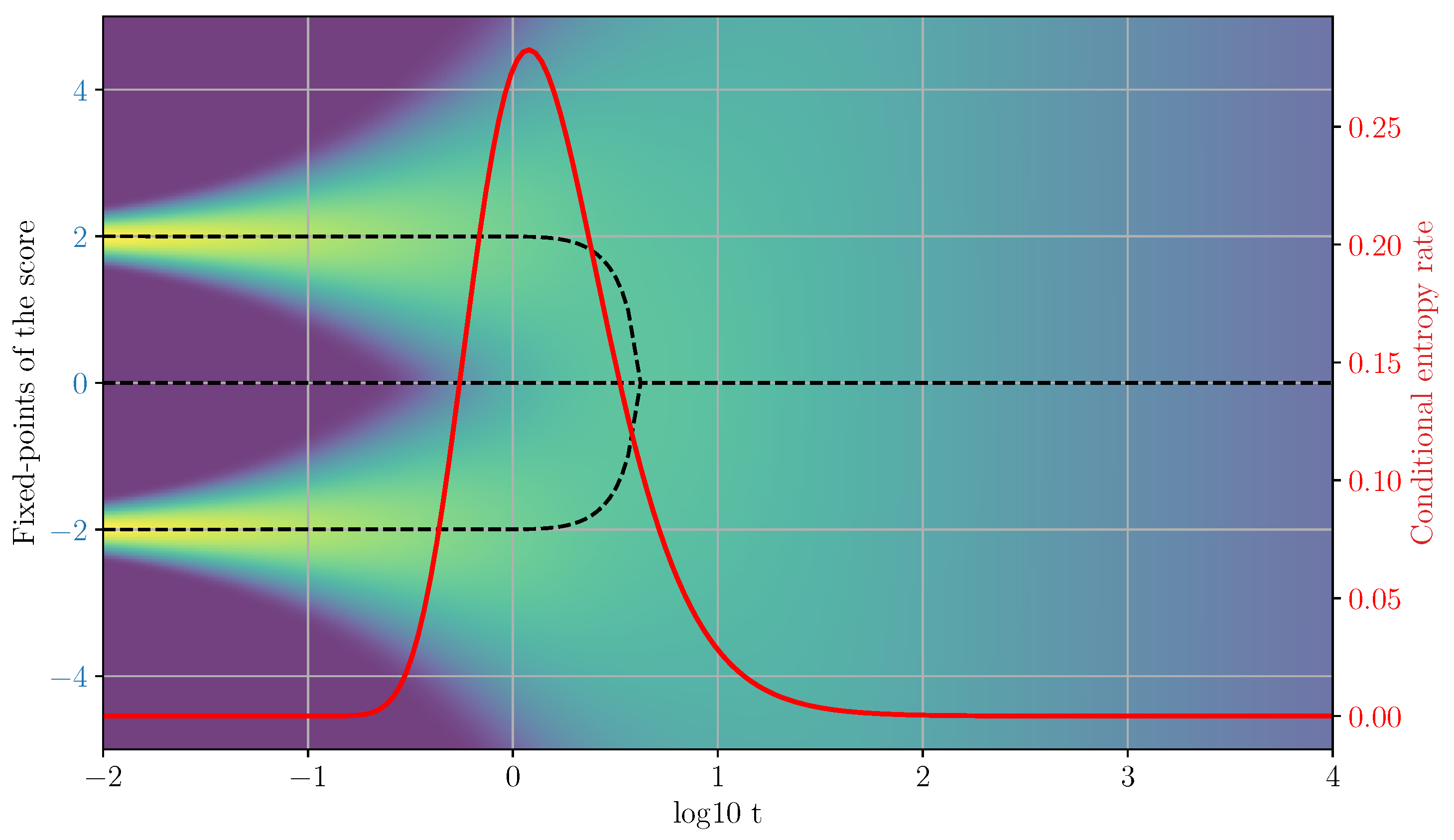
Figure 2.
Stability and instability of trajectories in different parts of a symmetry-breaking potential. Generative branching is associated with divergent trajectories.
Figure 2.
Stability and instability of trajectories in different parts of a symmetry-breaking potential. Generative branching is associated with divergent trajectories.
Disclaimer/Publisher’s Note: The statements, opinions and data contained in all publications are solely those of the individual author(s) and contributor(s) and not of MDPI and/or the editor(s). MDPI and/or the editor(s) disclaim responsibility for any injury to people or property resulting from any ideas, methods, instructions or products referred to in the content. |
© 2026 by the authors. Licensee MDPI, Basel, Switzerland. This article is an open access article distributed under the terms and conditions of the Creative Commons Attribution (CC BY) license (http://creativecommons.org/licenses/by/4.0/).
Copyright: This open access article is published under a Creative Commons CC BY 4.0 license, which permit the free download, distribution, and reuse, provided that the author and preprint are cited in any reuse.


