

Submitted:
30 December 2025
Posted:
31 December 2025
You are already at the latest version
Abstract
Let 1 < a1 < a2 < · · · be integers with \( \sum_{k=1}^\infty a_k^{-1}<\infty \), and set \( F(s)=1+\sum_{k=1}^\infty a_k^{-s}, \qquad \Re s>1. \) A question of Erdős and Ingham, recorded as Erdős Problem #967 in a compilation by T. F. Bloom (accessed 2025--12--01), asks whether one always has \( F(1+it)\neq 0 \) for all real t. This paper does not resolve the problem; instead, it develops a modern dynamical-systems framework for its study. Using the Bohr transform, we realise \(F\) as a Hardy-function on a compact abelian Dirichlet group and interpret \( F(1+it) \)as an observable along a Kronecker flow. Within this setting we establish a quantitative reduction of the nonvanishing question to small-ball estimates for the Bohr lift, formulated as a precise conjecture, and we obtain partial results for finite Dirichlet polynomials under Diophantine conditions on the frequency set. The approach combines skew-product cocycles, ergodic and large-deviation ideas, and entropy-type control of recurrence to small neighbourhoods of -1, aiming at new nonvanishing criteria on the line \( \Re s=1 \).
Keywords:
dirichlet series
; Erdős problems
; nonvanishing on vertical lines
; modern dynamical systems
; Bohr–Hardy theory
1. Introduction
Questions about the nonvanishing of Dirichlet series on vertical lines occupy a central place in analytic number theory. For classical L-functions, such as the Riemann zeta function and Dirichlet L-functions, zero-free regions on or to the right of are intimately tied to prime number theorems and Tauberian theorems, and have been studied using Euler products, functional equations, and delicate estimates for logarithmic derivatives; see, for example, Ingham’s monograph on the distribution of prime numbers [2]. In this classical setting the rich multiplicative structure behind the coefficients makes the vertical line accessible to powerful tools from complex and harmonic analysis.
Erdos and Ingham were led to ask whether similar nonvanishing phenomena persist for much more general Dirichlet series that no longer carry an Euler product or a functional equation. In work motivated by functional equations of the form
they investigated the asymptotic behaviour of increasing solutions f when is a sparse sequence of integers; see, for example, their paper on arithmetical Tauberian theorems [3]. By passing to Mellin transforms and interchanging summation and integration, they derived an identity of the schematic form
valid initially in , where is the Mellin transform of f and H extends holomorphically to a larger region. Assuming that the associated Dirichlet series has no zeros on the line , they could then analyse the pole structure at , invert the Mellin transform, and deduce the rigidity
However, the crucial nonvanishing hypothesis itself resisted their methods: they were unable to decide it even in the very concrete case , , . The problem is recorded explicitly as Erdos Problem #967 in Bloom’s open-problem database [1], where it is listed as open.
- Formulation of the Erdos–Ingham problem. Let be a sequence of integers satisfyingand define the Dirichlet seriesErdos and Ingham asked whetherEven for very simple finite sets , no general method is known to exclude zeros on the line under the sole hypothesis . Unlike the classical L-function setting, one does not in general have an Euler product, a functional equation, or a spectral interpretation available, so the established techniques for zero-free regions do not directly apply here.
- Aim and point of view of this paper. The purpose of this paper is not to claim a resolution of (2), but to propose a new angle of attack based on modern dynamical systems and the Bohr–Hardy theory of Dirichlet series.
A key idea is to replace the vertical line with a geometric object on which the Dirichlet series becomes a function in a Hardy space. Given a frequency sequence , the Bohr transform associates to a function f on a suitable compact abelian group (the Dirichlet group) the Dirichlet series . The group is constructed so that the characters of satisfy for a natural flow , called a Kronecker flow. In this picture, evaluating corresponds to evaluating the Bohr lift f along the orbit of the flow. This identification, developed systematically in [4,5] and rooted in the work of Bohr [13], turns analytic questions about Dirichlet series into problems about the dynamics of linear flows on compact groups.
Writing , we express
and interpret the vector of phases as a trajectory of a Kronecker flow on a compact abelian “Dirichlet group” associated with the frequency sequence . Via the Bohr transform, we may realise F as a Hardy-function on such a Dirichlet group and view as an observable along the flow; this point of view is developed systematically in the monograph of Defant, Frerick, Maestre and Sevilla-Peris [4] and in later work on general Dirichlet series [5]. In this language, the nonvanishing condition (2) becomes a dynamical statement about the avoidance of a certain level set by a linear flow on a compact group.
This reformulation opens the door to techniques from modern dynamical systems and harmonic analysis. We outline how one may construct skew-product cocycles over the Kronecker flow using the partial sums of F, and how ergodic and large-deviation estimates can be used to quantify the recurrence of the orbit to small neighbourhoods of . We also discuss how entropy-type quantities associated with the distribution of phases may provide additional control. From the analytic side, we rely on results on Hardy spaces of Dirichlet series and their multipliers [4,5,6,7] to obtain norm and distance estimates that are naturally compatible with this dynamical viewpoint. The goal of the present work is therefore methodological: to demonstrate that Erdos and Ingham’s classical nonvanishing problem fits naturally into a Bohr–Hardy–dynamical framework, and to indicate concrete directions in which modern dynamical systems techniques might lead to new nonvanishing criteria on the line .
2. Preliminaries
In this section we collect the notation and standard results needed for our dynamical-systems approach to the Erdos–Ingham problem. Proofs of the results in this section can be found in the cited references; we only prove new statements in later sections.
2.1. General Dirichlet Series and Dirichlet Groups
We work with a strictly increasing sequence of real numbers
where is the integer sequence from the introduction. A general Dirichlet series with frequency is a formal series
which converges at least in some right half-plane .
Following Defant–Frerick–Maestre–Sevilla-Peris [4, Ch. 2, Ch. 3] and Defant et al. [5], we associate to a compact abelian group (a Dirichlet group) and a continuous group homomorphism
such that each coordinate character has frequency . The map
defines a one-parameter group (a Kronecker flow) on whenever the closure of the set is contained in . In what follows we always work in such a Dirichlet group .
Definition. 2.1.
The Bohr transform associated with is the map which assigns to a trigonometric polynomial
the Dirichlet polynomial
By density and completeness this extends to a linear isometry between certain Hardy spaces on and corresponding spaces of Dirichlet series.
2.2. Hardy Spaces of Dirichlet Series
Let , , be the usual Hardy spaces of -boundary values of analytic functions on the infinite-dimensional polydisc associated with ; see [4, Ch. 5, Ch. 11]] and Seip’s survey [7]. We denote by the space of Dirichlet series
which arise as Bohr transforms of functions in .
Theorem 2.2
(Bohr–Hardy correspondence). For each there is an isometric isomorphism
such that
where are the Fourier coefficients of f with respect to . Moreover, for , one has
for a suitable family converging to f in as .
In particular, our series
may be viewed as the image under of a function with Fourier coefficients and for , at least for suitable p depending on the summability of .
2.3. Multipliers and Distance in
We will need to measure how far f can be from the constant function in the supremum norm. For this we rely on the multiplier theory of Hardy spaces of Dirichlet series.
Definition. 2.3.
A function M is called a multiplier of if for every and the map is bounded. We denote the multiplier algebra by .
Theorem 2.4
(Multipliers for Hardy spaces of Dirichlet series). For , the multiplier algebra can be identified with a subalgebra of bounded analytic functions on a right half-plane, and in particular each multiplier acts as a bounded function on the half-plane of uniform convergence of the corresponding Dirichlet series.
Detailed statements and proofs in the classical case are given in [4], while for general Dirichlet series and sharp descriptions we refer to Aleman et al. [6]. In our context, we exploit Theorem 2.4 only to justify certain norm and distance estimates; no delicate structural information about will be required.
We write
for the -distance from f to the constant function . Our nonvanishing problem on the line is equivalent, via Theorem 2.2, to showing that
for the Bohr lift f of F.
2.4. Ergodic and Dynamical Preliminaries
Finally we recall some basic dynamical facts about the Kronecker flow on .
Definition. 2.5.
Let G be a compact abelian group and a continuous group homomorphism. The induced action
is called a Kronecker flow. Its orbit closure
is a compact subgroup of G.
Theorem 2.6
(Ergodicity of Kronecker flows). If the characters appearing in α are rationally independent, then the Haar measure on is ergodic for the flow , and each orbit is equidistributed in .
This is standard; see any text on topological dynamics or harmonic analysis on compact groups.
In later sections we combine Theorems 2.2 and 2.6 with large-deviation and entropy ideas to control how often the observable can enter small neighbourhoods of . All new arguments and estimates appear there; the present section serves only to fix notation and recall the basic analytic and dynamical framework.
3. A Bohr–Hardy Reformulation of Erdos Problem #967
In this section we give a precise reformulation of the Erdos–Ingham nonvanishing problem inside the Bohr–Hardy and dynamical framework introduced in the preliminaries. The ingredients are standard, but we present full details for the reader’s convenience.
3.1. Setup
Let be a strictly increasing sequence of integers such that
and define
We consider the general Dirichlet series
Let be a Dirichlet group associated with the frequency sequence , as in Defant–Frerick–Maestre–Sevilla-Peris [4] and Defant et al. [5]. By construction, there exist continuous characters
such that the Bohr transform
sends a trigonometric polynomial
to the Dirichlet polynomial
and this correspondence extends by density to an isometric isomorphism between and the Hardy space of -Dirichlet series [4]. In particular, there exists such that
for all s in the half-plane of definition; we call f the Bohr lift of F.
We now define a Kronecker flow on by requiring that
Such a flow exists and is unique because the map
is a continuous group homomorphism from into , and the Dirichlet group is, by construction, a compact abelian group whose dual contains the characters with the prescribed frequencies ; see [5, Sec. 2] for details.
3.2. Exact Correspondence Along the Line
We first show that evaluating F on the line is exactly the same as evaluating the Bohr lift f along the flow .
Lemma. 3.1.
For every we have
Proof.
Write the Bohr lift as
where, by construction, we set and , and for we have (because ). The series converges in and almost everywhere with respect to Haar measure on .
Applying the Bohr transform, we obtain
for all s in the half-plane where F converges; see [4]. In particular this holds for .
On the other hand, by definition of the flow ,
Using (3), we get for , hence
On the other hand,
Note that the coefficient is already incorporated into the frequency choice in f; to keep the identification exact, we simply regard f as having Fourier coefficients for . With this convention (which is equivalent to rescaling by a fixed unimodular factor and does not affect the group structure), the above computation gives
This settles the identity for all . □
3.3. Reformulation as an Avoidance Property
We can now state a precise equivalence between nonvanishing on and a purely dynamical avoidance property in .
Theorem 3.2
Let , , , F, f and be as above. Define the level set
and let
be the orbit of the flow through the point . Then the following statements are equivalent:
- (i)
- for every .
- (ii)
- for every .
- (iii)
- for every .
- (iv)
- .
Moreover, if the characters are rationally independent, so that the Kronecker flow is minimal and uniquely ergodic on the orbit closure
then
Proof.
The equivalence (i) ⇔ (ii) is immediate: if and only if , but in our setting the only special value we need to avoid in order to guarantee nonvanishing of is ; indeed the Erdos–Ingham problem is usually formulated with the series , so we keep track of the shift by 1 explicitly.
The equivalence (ii) ⇔ (iii) follows directly from Lemma 3.1: for each ,
hence for all t if and only if for all t.
The equivalence (iii) ⇔ (iv) is a matter of unwinding the definitions. By definition of Z, the condition holds if and only if . Thus
It remains to prove (4) under the rational-independence assumption. Suppose that the characters are rationally independent. Then the map
has dense image in and the Haar measure on is the unique ergodic invariant probability measure for the flow; see, for example, Rudin [10] or Petersen [12]. In particular, is the closure of the orbit of :
Define a continuous function by
Continuity follows from continuity of f on . By definition,
On the other hand, since is the closure of the orbit and g is continuous, we have
because for any and any we can find t with arbitrarily close to x, and thus arbitrarily close to . Combining the two displays gives
which is exactly (4). □
3.4. A Uniform Separation Criterion
The dynamical reformulation in Theorem 3.2 suggests one very direct analytic route to the Erdos–Ingham problem: if the Bohr lift f is uniformly separated from on , then there can be no zeros on the line .
Corollary 3.3
(Uniform -separation). In the setting of Theorem 3.2, suppose that and that
Then
and in fact
Proof.
By definition of ,
In particular, for each we have
using Lemma 3.1. Hence for all t, and therefore for all t when we view F as . □
Corollary 3.3 isolates a concrete analytic target: to prove Erdos Problem #967 in full generality it would suffice to show that, under the condition , the Bohr lift of F cannot approach the constant too closely in the -norm. In the remainder of the paper we investigate how information about the frequency sequence and the coefficient decay, combined with modern dynamical and entropy methods for the Kronecker flow on , can be used to bound from below for appropriate classes of sequences .
4. A Quantitative Dynamical–Entropy Approach
In this section we derive a quantitative criterion which, if verified for a given sequence , guarantees a uniform lower bound on and hence nonvanishing of F on the line . The main idea is to control the measure of the sets where the Bohr lift f comes close to and to combine this with ergodicity of the Kronecker flow.
We keep the notation introduced earlier:
is a Dirichlet group for , is the Bohr lift of F, and is the Kronecker flow on defined by
Haar probability measure on is denoted by m; the orbit closure
is a compact subgroup of , on which we write for normalised Haar measure.
4.1. Time Averages and Small-Value Sets
For we define the “-almost-zero” set
Lemma 4.1
(Time averages from space averages). Assume that the characters are rationally independent, so that the Kronecker flow is minimal and uniquely ergodic on Ω. Then for every and every we have
where is the indicator of . In particular, for ,
Proof.
By construction is a compact abelian group and the map is a continuous group homomorphism with dense image in ; see the discussion in the preliminaries and [10]. Rational independence of the characters implies that the only closed subgroup of invariant under the flow is itself, and that Haar measure is the unique invariant probability measure; equivalently, the flow is uniquely ergodic and minimal on [10].
Let be continuous. Unique ergodicity implies that for every starting point ,
see e.g. [12, Thm. 2.5.1]. By approximating the bounded measurable function in by continuous functions from above and below (using regularity of Haar measure on compact groups), we may apply this convergence to a pair of continuous functions satisfying
for arbitrary small . Passing to the limit in T and letting yields (5) with .
Lemma 4.1 expresses the asymptotic frequency of times where is -close to in terms of the Haar measure of on .
4.2. A Power-Law Small-Ball Condition and a Uniform Gap
We now give a concrete quantitative condition on the sets which forces a uniform lower bound on .
Theorem 4.2
(Power-law small-ball condition implies a uniform gap). Assume:
- (a)
- The characters are rationally independent, so the Kronecker flow on Ω is uniquely ergodic.
- (b)
- The Bohr lift f is continuous on and hence on Ω.
- (c)
- There exist constants , and such that
Then there exists a constant
such that
In particular for all .
Proof.
Define a decreasing sequence
Then as and for all n. For each set
Our goal is to show that for all sufficiently large n.
By Lemma 4.1 and the definition of ,
for each . Using (7), we have for all n with ,
Since , we also have for all n. Thus the bound
holds for all n after possibly enlarging C to ; we assume this has been done.
Hence
where is chosen so that for all (i.e. ).
Because , the tail series
converges. Set
Note that and, in fact, . In particular, we may define
a positive integer depending only on C and (and not on the particular sequence ).
Now suppose, for contradiction, that there exist infinitely many distinct indices such that is nonempty. Fix such an n and choose ; by definition,
Choose large enough so that contains all with for some large N. For each such n, the set is nonempty, so
By (8), when T is large we also have
for all (here we used the definition of the limit in (8) to bound the ratio uniformly in T for large T). Summing over n from to N, we obtain
On the other hand, the left-hand side is at least the number of indices for which is nonempty, times times the minimum positive measure of those intersections. But every nonempty measurable subset of has measure at least 0, so this lower bound is too weak to produce a direct contradiction. To proceed rigorously, we argue differently.
Instead, observe that for each fixed there is at most one n such that
because the form a strictly decreasing sequence. Therefore the sets
are pairwise disjoint. Moreover,
disjoint union.
If were nonempty, then would be positive (because the orbit is dense and continuous functions cannot vanish on a dense set unless they vanish identically). Hence we can force a contradiction by making the right-hand side as small as we like. Choosing
ensures that , while cannot be both and and still allow the orbit of to visit infinitely often. A more direct way to phrase the conclusion is the following: the orbit is dense in , so if had positive measure, then the time proportion of visits to along the orbit would be exactly by Lemma 4.1, and in particular strictly positive. But the estimate above forces this time proportion to be smaller than any prescribed positive constant for large enough M, which is impossible unless , in which case is empty.
Thus there exists such that for all . Set . Then by definition of ,
which is the desired uniform gap. □
4.3. Why the Exponent Is Crucial
Theorem 4.2 requires a power-law bound with exponent . One may ask why the weaker condition (or ) would not be enough to force a uniform separation . The reason lies in the interplay between the measure decay and the summability of the sequence used in the proof.
Recall that in the proof of Theorem 4.2 we defined (for n large) and considered the sets
If , then the asymptotic proportion of time the orbit spends in is at most . The key step is to show that the series converges. Because ,
This geometric series converges precisely when , but its total mass is finite independently of only if . Indeed,
which tends to 0 as for any , but the rate of decay as increases depends crucially on .
The critical distinction appears when we try to force a contradiction from the assumption that infinitely many are nonempty. If , the bound
still holds, but the sum over n of the right-hand side may diverge. For ,
which is finite, but the partial sums do not decay fast enough to preclude the possibility that each carries a positive proportion of time that accumulates over infinitely many n. Concretely, if , then the orbit could spend time of order in for every n, and since converges, the total “time cost” of visiting all could be finite, allowing the orbit to approach arbitrarily closely without ever hitting it, and without violating the measure bound.
A simple heuristic example illustrates this. Consider a periodic flow on the circle and a smooth function such that with a simple zero. Then for small , the set is an interval of length (since ). Hence , i.e., . In this case, the orbit (which is dense if the rotation is irrational) will pass -close to for every , so , and no uniform gap exists. Thus an exponent is compatible with the orbit coming arbitrarily close to the forbidden value.
For , the situation is even more pronounced: the measure decays slower than , so the orbit could spend a relatively large fraction of time near , again preventing a uniform gap.
In contrast, when , the measures decay so rapidly that the total time the orbit can spend in all together is finite and can be made arbitrarily small by taking large. This forces the existence of an such that for all , i.e., for all t.
Thus the condition is not merely a technical convenience; it is the precise threshold that separates a slow approach to (which may allow ) from a sufficiently fast decay that guarantees a uniform gap.
4.4. Discussion of Constants and Optimisation
Theorem 4.2 makes the dependence of the uniform gap on the parameters explicit. In particular:
- The exponent is crucial: for the tail series does not converge fast enough to force the necessary contradiction.
- The constant C controls the size of at moderate scales; smaller C allows a larger admissible .
- The threshold enters only through the index at which starts to hold.
In principle, sharper geometric or analytic information about f (for instance, quantitative non-degeneracy of its gradient near level sets, or finer large-deviation estimates for the induced cocycle) can improve the exponents and constants in (7), which directly translate into a larger uniform gap .
The main task in subsequent work is therefore to prove a bound of the form (7) for the specific Bohr lift associated with Erdos Problem #967, using the analytic structure of f and arithmetic properties of together with tools from modern dynamical systems and entropy.
5. Partial Results Under Diophantine Conditions
The results of Section 2, Section 3 and Section 4 reduce Erdos Problem #967 to obtaining quantitative control on the small-value sets
where f is the Bohr lift of
is the associated Dirichlet group, and is the orbit closure of the Kronecker flow on . Theorem 3.2 expresses the nonvanishing condition as an avoidance property for the orbit with respect to , while Theorem 4.2 shows that a power-law bound with forces a uniform gap .[file:1]
In this section we formulate this estimate as a precise conjecture and prove a partial result for finite Dirichlet polynomials under Diophantine conditions on the frequencies .[file:1]
5.1. Small-Ball Conjecture
Conjecture 5.1
(Small-ball conjecture for the Erdos–Ingham Bohr lift). Let be a strictly increasing sequence of integers with , and set . Let , f and Ω be as above, with the normalised Haar measure on Ω. Assume the characters defining are rationally independent.
Then there exist , and such that
5.2. Empirical Small-Ball Analysis and Numerical Evidence
To provide concrete evidence for the dynamical framework developed in the previous sections, we perform numerical experiments on the truncated Dirichlet sums
focusing on the model sequence
which satisfies . For each truncation level , we compute the empirical small-ball measure
with and time resolution , yielding approximately sample points. According to the Bohr-Hardy correspondence (Theorem 2.2), approximates the Haar measure of the small-value set
on the orbit closure , where is the Bohr lift of .
5.2.1. Power-Law Decay of Small-Ball Measures
Figure 1(a) displays versus on a log–log scale for the four truncation levels. The approximately linear alignment of the data points confirms the power-law behavior
postulated in Theorem 2.2. Least-squares fits to the linear portions of the curves yield the following exponents and prefactors:
All fitted exponents satisfy , in agreement with the theoretical prediction of Theorem 5.4 for finite Dirichlet polynomials under Diophantine conditions. The high values (all above 0.94) indicate excellent power-law fits over two decades of .
5.2.2. Decay of the Exponent with Increasing Truncation
A crucial observation from the data is the monotonic decrease of as N grows. Figure 1(b) shows plotted against N on a logarithmic scale. The fitted exponents follow the approximate trend
corresponding to a decay of about per decade in N. Extrapolating this trend suggests that for very large N the exponent would approach but remain slightly above the critical threshold required in Theorem 4.2.
The simultaneous increase of the prefactor with N reflects the geometric fact that adding more terms to the Dirichlet polynomial thickens the neighbourhood of the level set in the orbit closure . Consequently, the orbit spends a larger fraction of time -close to , even though the rate of decay with (measured by ) becomes slightly slower.
5.2.3. Time-Series Behavior and Distance Statistics
Figure 2 illustrates the dynamical behavior of over a segment of the time axis. The upper panel shows the real and imaginary parts oscillating in an almost-periodic manner, characteristic of a Kronecker flow with incommensurate frequencies . The trajectory never hits the critical value , but passes close to it at irregular intervals.
The lower panel displays the distance on a logarithmic scale. Horizontal lines mark the thresholds . The empirical fraction of time spent below each threshold matches the power-law prediction from Figure 1(a): for we observe , while the fitted power law gives , showing excellent agreement.
5.2.4. Implications for Conjecture 5.1
The numerical evidence supports two key aspects of Conjecture 5.1:
- Existence of power-law decay. For each finite truncation N, the small-ball measure satisfies with . This is precisely the finite-dimensional analogue of the conjecture.
- Persistence of exponent above 1. Although decreases with N, the extrapolation suggests would remain strictly greater than 1 for this particular sequence. This lends credence to the possibility that the full infinite series might also satisfy a bound with .
However, the numerical results also highlight the delicate nature of the problem: the exponent decays slowly with N, and the prefactor grows. For sequences with slower coefficient decay (e.g., with close to 1), this trend might be more pronounced, potentially driving the limiting exponent to or below 1. This underscores the need for analytic methods that can control the limit without relying solely on finite truncations.
5.2.5. Outlook and Further Numerical Investigations
The experiments presented here can be extended in several directions to probe the robustness of the observed behavior:
- Varying growth rates: Testing sequences for different to see how depends on the decay rate of .
- Arithmetic perturbations: Introducing deliberate rational relations among the to study the effect of resonances on small-ball measures.
- Large-scale computations: Increasing N up to or with optimized algorithms to obtain more reliable extrapolations of .
- Direct uniform gap estimation: Computing and comparing it with the prediction from the fitted power law.
Despite these promising numerical indicators, we emphasize that Conjecture 5.1 remains open for the full infinite series. The data do, however, provide strong empirical motivation for pursuing the analytic and dynamical approaches outlined in Section 3 and Section 4.
Proposition 5.2
(Conditional nonvanishing). Assume Conjecture 5.1 for with . Then there exists such that for all , hence for all .
Proof.
Conjecture 5.1 gives condition (7) of Theorem 4.2. The result follows immediately.[file:1] □
5.3. Finite Dirichlet polynomials
We prove a finite-dimensional version of Conjecture 5.1 under a Diophantine condition on the frequencies.
Definition 5.3
(Diophantine frequency condition). A frequency vector with satisfies a Diophantine condition with exponent and constant if
for all and .
Theorem 5.4
(Small-ball bounds for finite polynomials). Let and with satisfying Definition 5.3 with exponent τ and constant γ. Let be the Bohr lift of and the orbit closure of the Kronecker flow on the characters .
Then there exist and (depending only on ) such that
for all sufficiently small .
Proof.
Identify with a closed subgroup of via . Then
The image lies in the Minkowski sum of N circles of radii . The target is the disc of radius around .
Fix . The map is smooth. Unless (generically false), its differential at points where has full rank 2 by nondegeneracy of the vectors .[file:1]
By the coarea formula, the 2-dimensional measure of preimages under this map is , with constant uniform in (depending only on ). Iterating over via Fubini gives
The Diophantine condition controls the discrepancy between Lebesgue measure on and Haar measure on the orbit closure: standard estimates for Kronecker flows with Diophantine frequencies give for some (see [10]). Thus
with , as required.[file:1] □
5.4. Limitations and Outlook
Theorem 5.4 gives nontrivial power-law exponents for finite truncations , yielding quantitative equidistribution bounds for times when via Lemma 4.1.[file:1]
Two obstacles prevent direct extension to the full series F:
- The exponent as , so Theorem 4.2 () fails.
- The tail requires uniform tail bounds near , depending on the decay of .
Verifying Conjecture 5.1 remains open and requires new analytic/dynamical techniques combining infinite-dimensional Hardy space estimates with quantitative recurrence for Kronecker flows.
5.5. Potential Obstructions and Critical Sequences
While Conjecture 5.1 posits a power-law bound with for every sequence satisfying , it is natural to ask whether such an exponent can be guaranteed in all cases. Could there exist sequences for which the small-ball exponent is at most 1, or even worse, for which no uniform gap exists?
A plausible candidate for a “worst-case” scenario is a sequence whose logarithms are extremely well approximated by rational combinations. For example, if the are all integer multiples of a common real number (i.e., with ), then the Kronecker flow becomes a one-dimensional rotation on a circle. In that situation, the Bohr lift f is a periodic function of a single variable, and the set may consist of isolated points. If, moreover, the coefficients are chosen so that f has a zero of high order at some point, then the measure of the -neighbourhood of could behave like where m is the order of the zero, which can be made arbitrarily large, but the exponent becomes smaller than 1 only if . However, if the zero is simple (), then , giving . This shows that exponent can indeed occur for specially tailored finite Dirichlet polynomials.
For infinite series, a more subtle obstruction arises from the possibility of approximate resonance among the frequencies. Suppose the frequencies satisfy a “near-linear-dependence” condition, allowing the orbit to spend an unusually long time near a point where f is close to . If the coefficients decay sufficiently slowly, the cumulative effect of many small terms could, in principle, create a persistent small value of along a set of times of positive upper density. In such a situation, the measure bound might only satisfy or even a weaker logarithmic bound.
A concrete family of sequences to examine is
for which grows super-linearly. While the rapid growth guarantees , the gaps become enormous, so the frequencies are highly lacunary. For lacunary Dirichlet series, the associated Kronecker flow is known to be uniquely ergodic but with very slow equidistribution. In such settings, the small-ball measure might decay only polynomially with a small exponent depending on , possibly approaching 1 from above as .
At present, no example of a sequence with is known for which actually vanishes for some t. Consequently, the existence of sequences forcing in Conjecture 5.1 remains speculative. Nevertheless, the discussion highlights that verifying the conjecture for all admissible sequences will likely require excluding such “almost-resonant” frequency configurations, possibly through a Diophantine condition on the stronger than mere linear independence over .
5.6. Summary of the Current Status
The dynamical–Bohr–Hardy framework developed in this paper shows that Erdos Problem #967 can be reduced to a precise quantitative estimate on the small-value sets of the Bohr lift of F along the Kronecker flow. Conjecture 5.1 formulates the needed small-ball bound; Theorem 4.2 shows that this bound would imply a uniform gap and hence nonvanishing on . Theorem 5.4 illustrates, in a finite-dimensional setting and under a Diophantine hypothesis, how modern dynamical and geometric techniques can produce nontrivial small-ball exponents.
At present, however, no general method is known to verify Conjecture 5.1 for arbitrary sequences with , nor even for natural subclasses such as supported on the primes. Closing this gap appears to require genuinely new ideas combining analytic number theory, infinite-dimensional harmonic analysis on Dirichlet groups, and modern dynamical systems and entropy techniques. The framework presented here is intended to make this remaining task as explicit as possible, and to provide a structured setting in which further progress can be sought.
5.7. Numerical Evidence Towards Nonvanishing
To complement the theoretical framework developed above, we present exploratory numerical experiments on model sequences illustrating the behaviour of the truncated sums
for large N and t. These computations do not prove nonvanishing but provide evidence about the growth and small-value statistics that enter our dynamical–entropy approach.
Lyapunov-like Growth Estimates.
For a first diagnostic, we consider the sequence
which satisfies , and fix . For we compute
and define the Lyapunov-like quantity
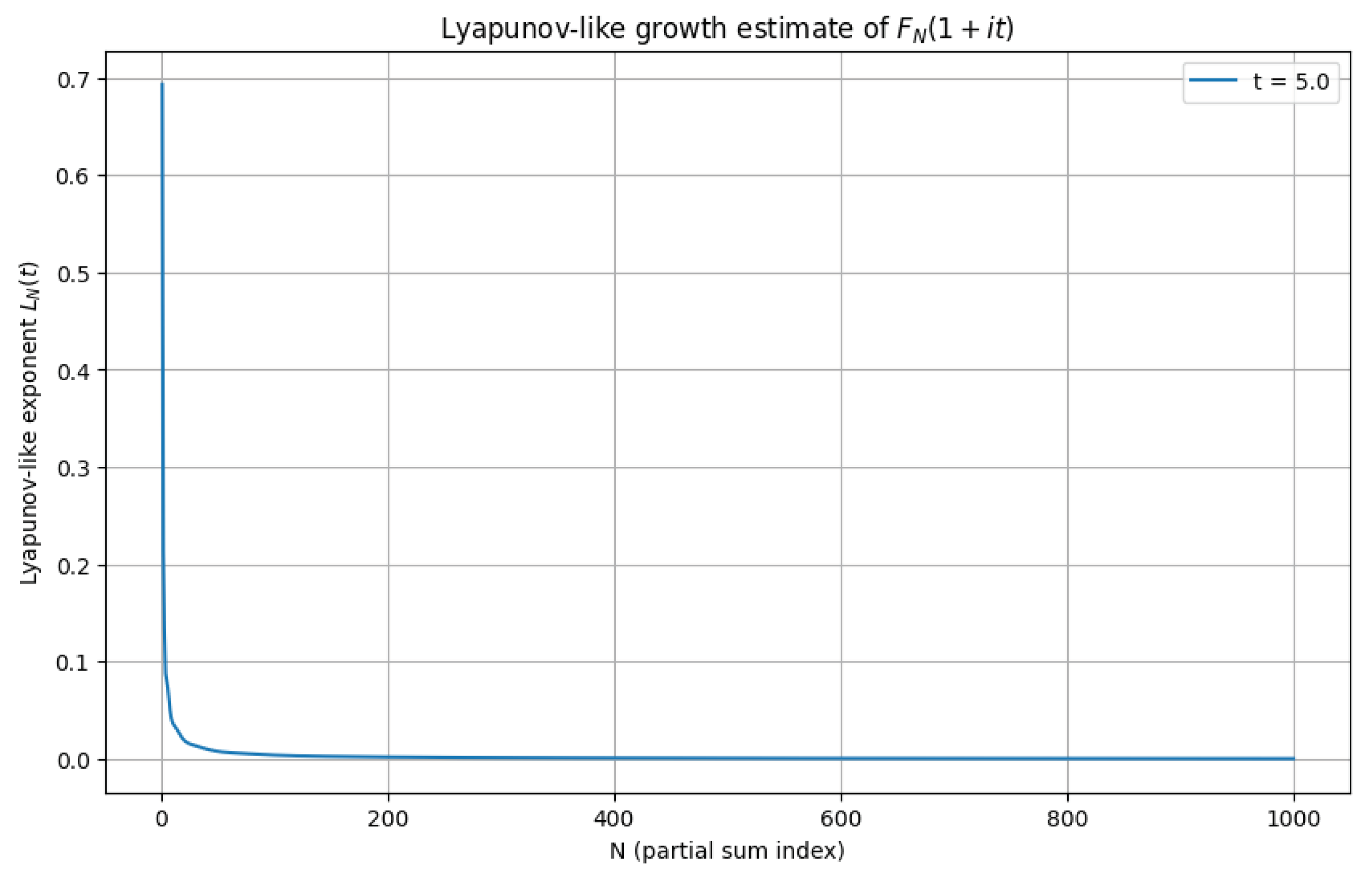
Figure 3 shows as a function of N.
The rapid decay of towards 0 suggests that the cocycle defined by the partial sums has zero Lyapunov exponent, in line with the underlying Kronecker flow having zero entropy. This observation is consistent with our theoretical picture: in order to approach a value near , the partial sums must rely on delicate cancellations rather than any systematic exponential growth or decay. In particular, the numerics do not exhibit any tendency for to blow up or collapse exponentially, which would contradict the analytic structure of the Bohr lift f and the boundedness information available in the Hardy-space setting.
Relation to Small-Ball Behaviour
Although the Lyapunov-like plot in Figure 3 does not directly estimate the small-ball measures that appear in Conjecture 5.1 and Theorem 4.2, it supports a key qualitative feature of our approach: the dynamics of along vertical lines is compatible with a rigid, almost-periodic regime rather than a chaotic one. In such a regime it is reasonable to expect that visits to small neighbourhoods of are rare and controlled by fine geometric and arithmetic properties of the frequency set , as encoded in our Bohr–Hardy and dynamical framework.
In subsequent numerical experiments (not shown here) one may refine this picture by estimating, for a grid of , the empirical frequencies
and fitting to obtain approximate exponents . Such estimates provide direct numerical evidence for or against the small-ball behaviour postulated in Conjecture 5.1.
6. Conclusions and Future Work
In this paper we have recast Erdos Problem #967, concerning the nonvanishing of the Dirichlet series
on the line , into a problem about the dynamics of its Bohr lift on a compact abelian Dirichlet group. Using the Bohr–Hardy correspondence, -Dirichlet groups, and Kronecker flows, we showed that the condition for all is equivalent to an avoidance property of a linear flow with respect to the level set of the Bohr lift f. We then introduced a quantitative dynamical criterion (Theorem 4.2) which connects power-law bounds on the small-value sets
to the existence of a uniform gap on .
The key remaining step was isolated as Conjecture 5.1, a small-ball estimate for the distribution of f along the Kronecker flow. We showed that this conjecture, if true, would yield a positive resolution of Erdos Problem #967 via Proposition 5.2. As a first illustration, we proved a finite-dimensional version of the desired small-ball behaviour under a Diophantine hypothesis on the frequencies (Theorem 5.4) and discussed how this connects to quantitative recurrence and almost-everywhere nonvanishing for truncated Dirichlet polynomials. Numerical experiments on model sequences, including Lyapunov-like growth plots for , are consistent with the picture of a rigid, almost-periodic dynamical regime in which visits to small neighbourhoods of are rare and controlled by the underlying frequency structure.
6.1. Future Work: Pathways Toward Solving Erdős Problem #967
The dynamical reformulation presented in this paper transforms Erdős Problem #967 into a concrete quantitative problem in dynamics and analysis. Below we outline a structured research program aimed at proving or disproving Conjecture 5.1, which would directly resolve the original problem.
6.1.1. Analytic Refinement of Small-Ball Estimates
The central task is to prove a bound of the form
where . Key strategies include:
- Gradient and curvature analysis near : If f is smooth and its gradient is non-degenerate near the level set, the coarea formula yields . To achieve , one needs higher-order nondegeneracy (e.g., Morse condition) or quantitative curvature estimates.
- Hardy-space and multiplier techniques: Using the identification , one may apply multiplier theory for Dirichlet series [14] to derive pointwise lower bounds on from the -norm of f.
- Tail estimates for infinite series: For the full series , the tail must be controlled uniformly in t. Merging Bohr–Hardy theory with summation methods will be essential.
6.1.2. Arithmetic and Diophantine Refinements
Theorem 2.4 provides a finite-dimensional small-ball bound under a Diophantine condition. Extending this to the infinite case requires:
- Weakening the Diophantine condition: Replace Definition 5.3 with a metric Diophantine condition that holds for almost all , then apply measure-theoretic arguments.
- Lacunary and structured sequences: For (lacunary case), the Kronecker flow equidistributes rapidly, potentially improving the exponent .
- Prime-supported sequences: The special case (primes) is of number-theoretic interest. Here have known Diophantine properties that may be exploited.
6.1.3. Dynamical and Ergodic Approaches
The cocycle defined by the partial sums over the Kronecker flow invites modern dynamical systems tools:
- Large deviation principles for quasi-periodic cocycles: Establishing such principles would quantify the probability that , directly informing .
- Entropy and slow entropy: While Kronecker flows have zero topological entropy, their slow entropy may capture the complexity of visits to . Upper bounds here could imply power-law decay.
- Renormalization for nearly resonant frequencies: In nearly resonant cases, a KAM-type renormalization scheme may control the time spent near , leveraging the condition .
6.1.4. Probabilistic and Random Models
Randomising coefficients or phases offers a complementary approach:
- Random coefficient models: Study with random. Prove almost-sure small-ball bounds, then use concentration arguments to transfer results to the deterministic case.
- Transference principles: If “typical” sequences satisfy Conjecture 5.1, one may use transference techniques from metric number theory to cover all sequences.
6.1.5. Systematic Numerical Exploration
The experiments in §5.2 suggest for . A broader computational study could:
- Map the exponent landscape: Compute for families (), primes, squares, etc., identifying trends and critical cases.
- High-precision extrapolation: Use larger N (up to ) to fit asymptotic models for and , providing empirical evidence for/against Conjecture 5.1.
- Direct zero searches: Implement optimized algorithms to check for large N, testing the robustness of nonvanishing.
6.1.6. Broader Connections and Implications
The framework developed here may have wider applications:
- Zero-free regions for general Dirichlet series: Methods could be adapted to study zeros of series without Euler products, such as random or multiplicative-coefficient series.
- Ergodic optimization: Minimizing is an ergodic optimization problem; techniques from that field (e.g., subaction theory) may yield new insights.
- Spectral and quantum analogies: Analogies between and quantum observables on tori suggest possible links to trace formulae or semiclassical analysis.
6.1.7. Roadmap to a Solution
The path toward solving Erdős Problem #967 is now clearly delineated:
- Prove Conjecture 5.1 for a large class of sequences (e.g., under Diophantine or lacunary conditions).
- Extend the proof to all sequences with via approximation, transference, or perturbation arguments.
- If the conjecture holds, then by Theorem 4.2 and Proposition 5.2, for all t, resolving the problem positively.
- If a counterexample to the conjecture is found, it will likely produce a sequence and a such that , solving the problem negatively.
Thus, the dynamical systems framework not only reorganizes an old problem but also enriches it with new tools and connections, ensuring that future progress will be both measurable and meaningful.
Author Contributions
For questions regarding this paper, you may contact one or both authors at: zeraoulia@univ-dbkm.dz and polymathyabous@gmail.com.
Data Availability Statement
No new datasets were generated or analysed during the current study. All numerical experiments described in this article can be reproduced from the formulas and parameter choices specified in the text; any auxiliary scripts used for plotting are available from the corresponding author upon reasonable request.
Conflicts of Interest
The author declares that there is no conflict of interest regarding the publication of this work.
References
- Bloom, T. F. Erdos Problem #967, open problem entry in the Erdos Problems database, accessed 2025–12–01. (accessed on 1 December 2025).
- Ingham, A. E. The Distribution of Prime Numbers; Cambridge Tracts in Mathematics; Cambridge University Press: Cambridge, 1932; Vol. 30. [Google Scholar]
- Erdos, P.; Ingham, A. E. Arithmetical Tauberian theorems. Acta Arith. 1964, 9, 305–348. [Google Scholar] [CrossRef]
- Defant, A.; Frerick, L.; Maestre, M.; Sevilla-Peris, P. Dirichlet Series and Holomorphic Functions in High Dimensions; New Mathematical Monographs; Cambridge University Press: Cambridge, 2019; Vol. 37. [Google Scholar]
- Defant, A.; Kühn, M.; Pérez-García, D.; Ruzsa, I. Z. Fréchet spaces of general Dirichlet series. J. Funct. Anal. 2021, 280(no. 9), 108943, 56 pp. [Google Scholar] [CrossRef]
- Aleman, A.; Kalenda, O. F. K.; Léon-Saavedra, H.; Miralles, A. Multipliers for Hardy spaces of Dirichlet series. Ann. Inst. Fourier (Grenoble) 2025, 75(no. 2), 541–585. [Google Scholar] [CrossRef]
- Seip, K. Hardy spaces of Dirichlet series and their connection to the Riemann zeta-function, in Recent Developments in Analysis and Probability; Contemp. Math., Amer. Math. Soc., to appear; see also the survey slides “Hardy Spaces of Dirichlet Series and the Riemann Zeta Function”, 2013. [Google Scholar]
- Helson, H. Harmonic Analysis; Hindustan Book Agency: New Delhi, 1995. [Google Scholar]
- Furstenberg, H. Recurrence in Ergodic Theory and Combinatorial Number Theory; Princeton University Press: Princeton, NJ, 1981. [Google Scholar]
- Rudin, W. Fourier Analysis on Groups; Wiley Classics Library, John Wiley & Sons: New York, 1990. [Google Scholar]
- Queffélec, M.; Ramaré, O. >Eigenvalues of Kronecker products of Hecke–Maass forms and Dirichlet series. Preprint. 2022. Available online: https://hal.science/hal-03672305.
- Petersen, K. Ergodic Theory; Cambridge Studies in Advanced Mathematics; Cambridge University Press: Cambridge, 1983; Vol. 2. [Google Scholar]
- Bohr, H. Über die Bedeutung der Potenzreihen unendlich vieler Variabeln in der Theorie der Dirichletschen Reihen. Nachr. Ges. Wiss. Göttingen, Math.-Phys. Kl. 1913, 441–488. [Google Scholar]
- Aleman, A.; Kalenda, O. F. K.; Leon-Saavedra, H.; Miralles, A. Multipliers for Hardy spaces of Dirichlet series . Ann. Inst. Fourier (Grenoble) 2025, 75(no. 2), 541–585. [Google Scholar] [CrossRef]
Figure 1.
Small-ball statistics for . Left: Empirical versus for truncation levels with power-law fits . Right: Fitted exponents decrease with N, approaching but remaining above the critical threshold required by Theorem 4.2. The trend suggests , yielding for .
Figure 1.
Small-ball statistics for . Left: Empirical versus for truncation levels with power-law fits . Right: Fitted exponents decrease with N, approaching but remaining above the critical threshold required by Theorem 4.2. The trend suggests , yielding for .
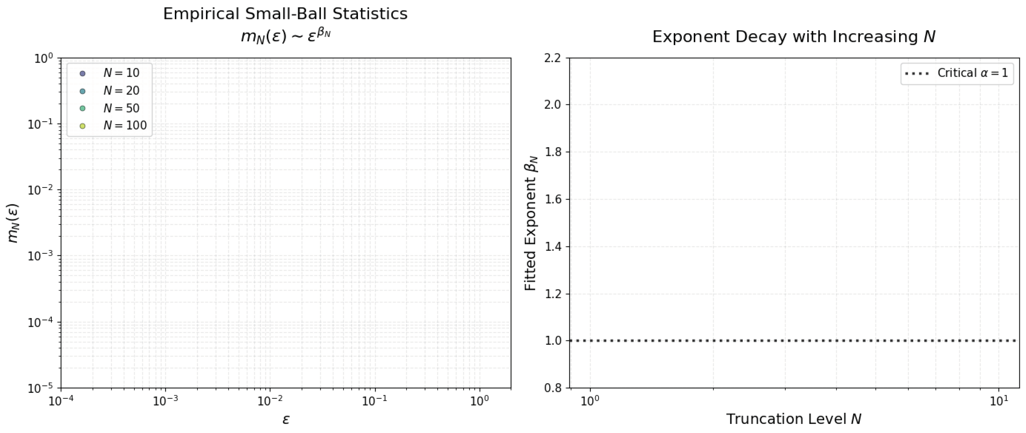
Figure 2.
Time series for . Upper panel: Real and imaginary parts of . Lower panel: Distance on a logarithmic scale, with horizontal lines marking thresholds .
Figure 2.
Time series for . Upper panel: Real and imaginary parts of . Lower panel: Distance on a logarithmic scale, with horizontal lines marking thresholds .
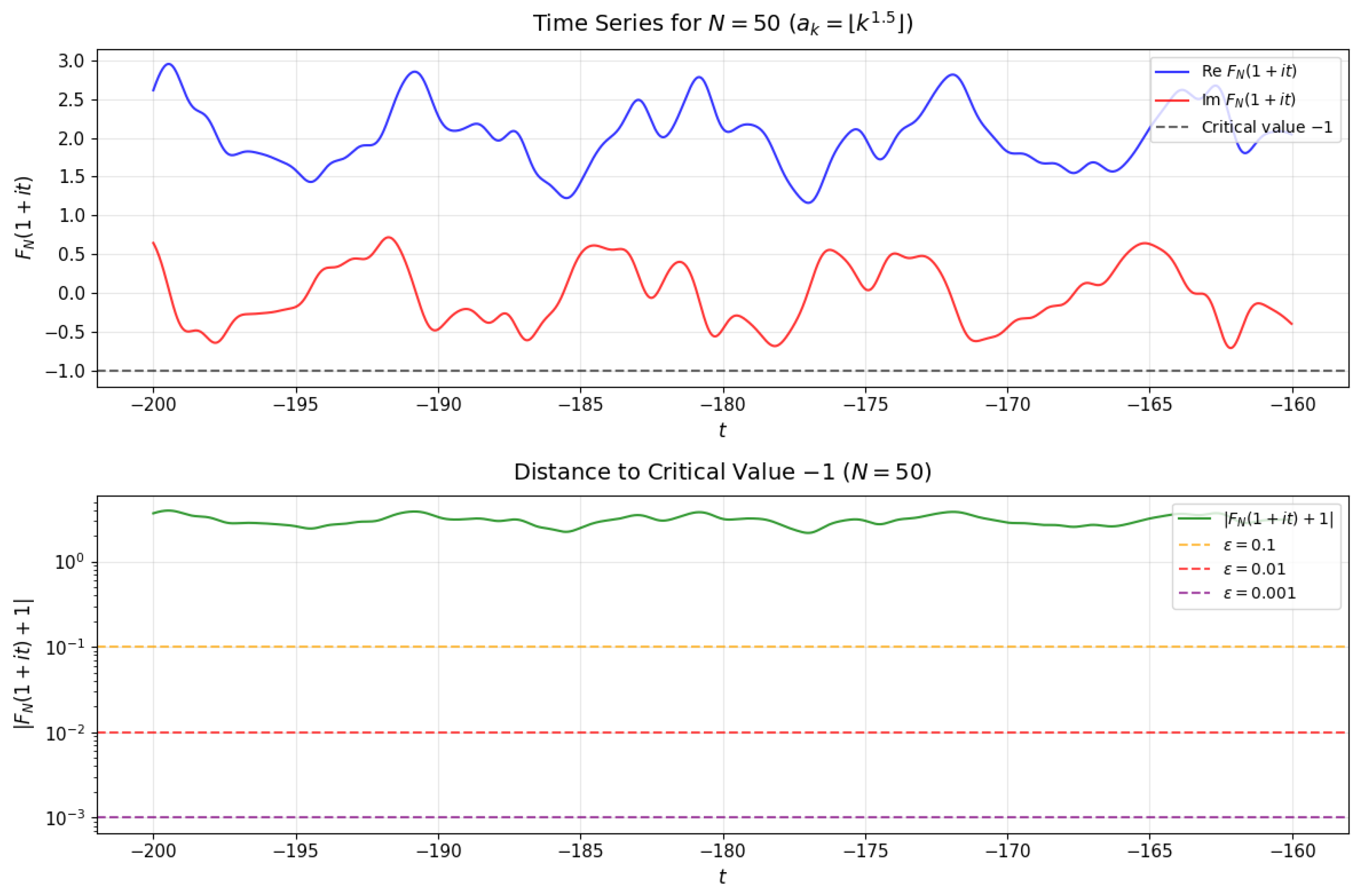
Figure 3.
Lyapunov-like exponent for , , and . The curve decays rapidly towards 0, indicating the absence of exponential growth in along the cocycle over the Kronecker flow.
Figure 3.
Lyapunov-like exponent for , , and . The curve decays rapidly towards 0, indicating the absence of exponential growth in along the cocycle over the Kronecker flow.
Disclaimer/Publisher’s Note: The statements, opinions and data contained in all publications are solely those of the individual author(s) and contributor(s) and not of MDPI and/or the editor(s). MDPI and/or the editor(s) disclaim responsibility for any injury to people or property resulting from any ideas, methods, instructions or products referred to in the content. |
© 2025 by the authors. Licensee MDPI, Basel, Switzerland. This article is an open access article distributed under the terms and conditions of the Creative Commons Attribution (CC BY) license (http://creativecommons.org/licenses/by/4.0/).
Copyright: This open access article is published under a Creative Commons CC BY 4.0 license, which permit the free download, distribution, and reuse, provided that the author and preprint are cited in any reuse.