Preprint
Review

This version is not peer-reviewed.

From Neurons to Networks: A Holistic Review of Electroencephalography (EEG) from Neurophysiological Foundations to Advanced Decoding

Submitted:

29 December 2025

Posted:

30 December 2025

You are already at the latest version

Abstract

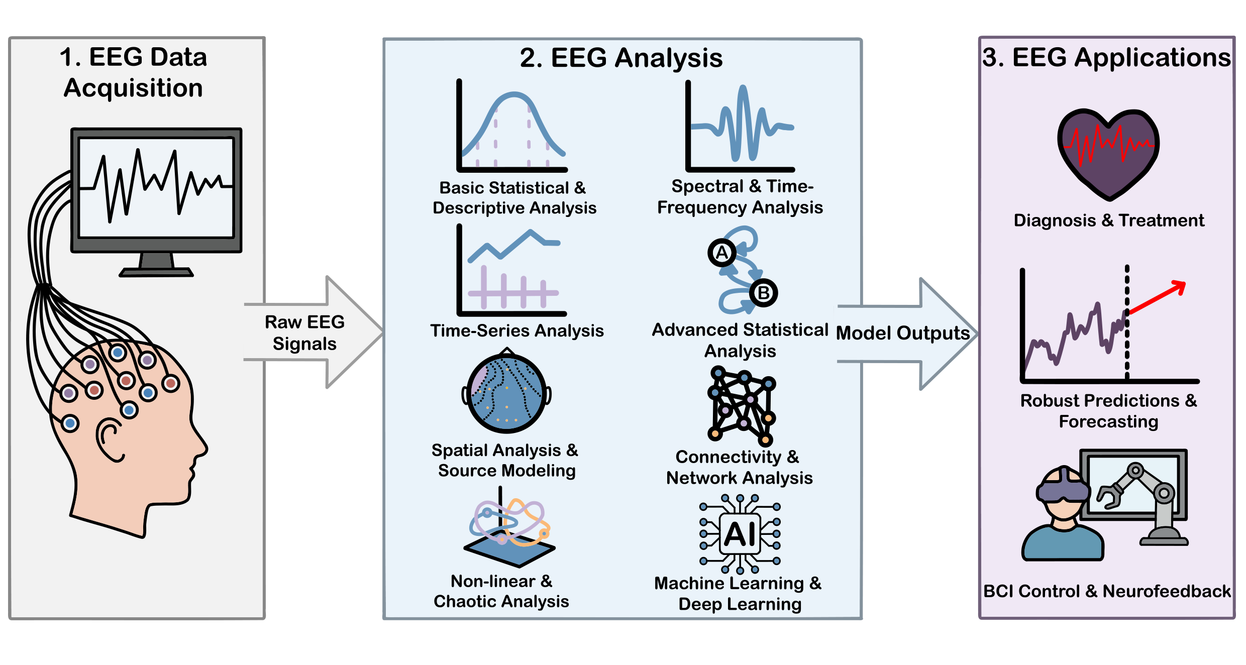
Electroencephalography (EEG) has transitioned from a subjective observational method into a data-intensive analytical field that utilises sophisticated algorithms and mathematical modeling. This progression encompasses developments in signal preprocessing, artifact removal, and feature extraction techniques including time-domain, frequency-domain, time-frequency, and nonlinear complexity measures. To provide a holistic foundation for researchers, this review begins with the neurophysiological basis, recording technique and clinical applications of EEG, while maintaining its primary focus on the diverse methods used for signal analysis. It offers an overview of traditional mathematical techniques used in EEG analysis, alongside contemporary, state-of-the-art methodologies. Machine Learning (ML) and Deep Learning (DL) architectures, such as Support Vector Machines (SVMs), Convolutional Neural Networks (CNNs), and transformer models, have been employed to automate feature learning and classification across diverse applications. We conclude that the next generation of EEG analysis will likely converge into Neuro-Symbolic architectures, synergising the generative power of foundation models with the rigorous interpretability of signal theory.

Keywords: 
;  ;  ;  ;  ;  ;  

1. Introduction

Electroencephalography (EEG) has substantially evolved throughout the years. The incorporation of mathematical tools and computational models has enabled researchers to gain a profound insight into brain function and its applications now encompass a wider array of fields. The study of biomedical signals draws upon multiple disciplines such as biology, biochemistry, neuroscience, medicine, engineering, mathematics and computer science, rendering it as one of the most fascinating areas of research. From a biological and neuroscience point of view, EEG signals elucidate neuronal dynamics that can be proven pivotal in diagnosis and treatment of many neuropsychiatric conditions. From a mathematical and signal processing point of view, they represent a highly complex and information-rich class of signals that can be challenging to interpret. This is because they are intricate by nature, for they are the result of million neurons’ activity which create a non-stationary, nonlinear and temporally dynamic signal [1]. In addition, the useful signal is often submerged in a highly noisy background originating from various sources. For this reason, sophisticated pre-processing techniques are considered imperative to isolate brain activity [2]. Finally, the relationship between the observed electrical potentials in the head and the underlying neurophysiological processes is not direct or simple, as the signal has a complex spatial topography and it is a multi-faceted outcome derived from the interactions of the brain sources [3].
These properties make clinical analysis vulnerable to subjectivity and require advanced computing tools for the reliable and quantitative extraction of diagnostically important information. For these reasons, in recent years, many researchers have been working to advance the methods for processing biomedical signals [4,5,6,7,8]. Basic descriptive statistics provide essential baselines for artifact detection and signal quality assessment, while spectral and time-frequency analysis methods allow for the precise characterisation of oscillatory power dynamics across different brain states [9]. Furthermore, time series analysis techniques [10] and advanced statistical methods [11], are utilised to model the temporal evolution of the signal for forecasting and feature extraction. To map these temporal dynamics to anatomical substrates, spatial analysis and source modeling techniques [12] are used. Connectivity and network analysis employs graph theoretical metrics to quantify the functional integration and information flow between these distributed regions [13]. Additionally, recognising the brain’s complex dynamical nature, nonlinear and chaotic analysis methods are increasingly applied to detect pathological changes in signal complexity [14]. However, the current state of the field is witnessing a paradigmatic shift from these traditional methods toward “Large EEG Models” and Generative AI [15]; while foundation models like LaBraM [16] and Gram [17] leverage massive pre-training on thousands of hours of data to achieve universal cross-subject generalisation and diffusion models [18] enable the direct reconstruction of visual stimuli from neural signals. Consequently, this review aims to describe the fundamental methods and techniques used in EEG analysis, while enabling the researcher to develop a comprehensive understanding of the whole field.

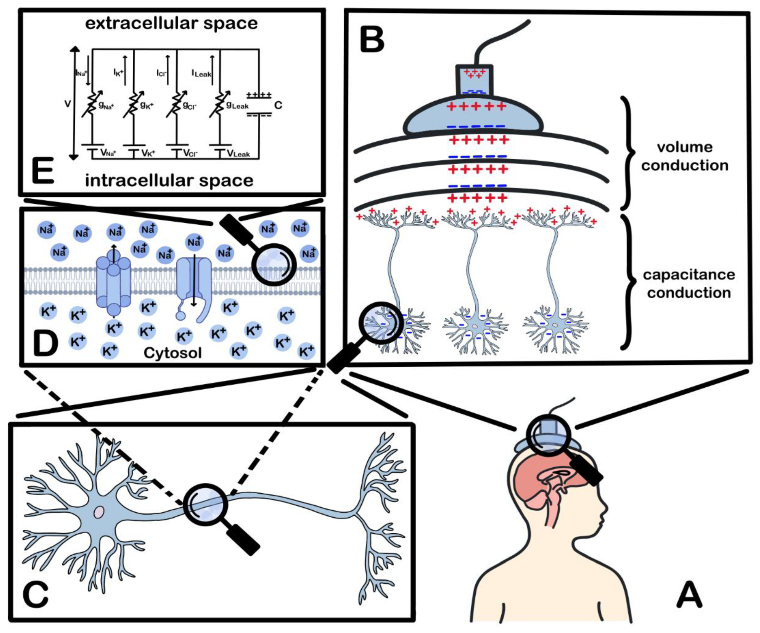
2. Biophysical Principles and Neurophysiological Basis

EEG records the temporal changes in the brain’s electric field, which arise from the sum of extracellular currents associated with the postsynaptic potentials of neurons. The recorded signal is a result not only of endogenous neuronal activity, but also of the electrical properties of the tissues (brain, bone, skin) that function as a potential conductor, as well as the orientation of the sources with respect to the surface of the head. The human brain consists of tens of billions of neurons and glial cells. The basis of electrical activity is the membrane potential ( V m 70   mV ) [19], which is due to the difference in ion concentration K + , Na + , Cl - , Ca 2 + inside and outside the membrane and it is regulated by active pumps e . g . ,   Na + /   K + - ATPase and passive ion channels. The action potential is a rapid change in this membrane voltage that transmits information along the neuronal terminals.
The Hodgkin-Huxley (HH) model [20,21,22] is a Nobel Prize winning mathematical model that faithfully describes the mechanism of generation and propagation of action potentials in nerve cells. This model was not just a description, but a predictive theory that laid the foundation for modern computational neuroscience. Hodgkin and Huxley’s basic idea was this: The action potential arises from changes in the permeability of the neuron’s membrane to specific ions ( Na +   and   K + ) , which are controlled by voltage-gated ion channels. Imagine the neuron’s membrane as a battery with many small switches (the channels). At rest ( 70   mV ) : K + channels are closed, Na + channels are tightly closed (but ready to open). When the potential exceeds a threshold ( 55 mV ) , the Na + channels open rapidly (depolarisation). Positive Na + ions flow into the cell, further uncoupling the potential ( + 40 mV ) . This is the anodic phase of the spike. Then, the Na + channels begin to close after a short period of time and the slowly activated K + channels open fully, driving the potential below the normal resting potential, before returning to its original value (refractory period) [23]. This choreography of opening and closing of the channels is what produces the action potential. For an intuitive approach to the Hodgkin-Huxley model, refer to the Appendix A.
The transmission of electrical signals in the brain is explained by the principle of volume conduction [24,25]. According to this, electrical charges interact following the well-known laws of electrostatics: opposite charges attract and like repel. Volume conduction is the process by which a group of ions repels neighboring ions with the same charge. These, in turn, repel subsequent ions, creating a “wave” of charge that moves through the extracellular space. Since the brain is not homogeneous, variations in tissue density can either facilitate or hinder the flow of ions. Furthermore, a signal from a large source (large dipole) can travel a much greater distance than a signal from a small source. To record such a signal from an electrode on the scalp, it must first traverse several layers: from brain tissue, dura mater, skull bone, skin, and hair, until it finally reaches the electrode. At the boundaries between different tissues, where volume conduction ceases, the signal is transmitted through the phenomenon of capacitive coupling. At these points, energy advantages are created, where charges accumulate on one side of an insulating barrier (e.g., bone) and, through electrostatic repulsion, cause the movement of like charges on the opposite side. The succession of these layers (brain, meninges, skull, skin, etc.) creates a series of such capacitors [26]. Figure 1 illustrates multi-scale electrical conduction.
A great review [27] attempts a unified and deep understanding of the biophysical mechanisms that generate extracellular electric fields and currents (e.g., EEG, LFP, ECoG). According to this work, extracellular fields do not originate exclusively from synaptic currents but are the result of the superposition of all active transmembrane currents, including action potentials Na + a n d Ca 2 + s p i k e s , intrinsic membrane currents (ionic currents that flow through voltage-gated channels of the neuronal membrane and are not directly induced by synaptic activity), and afterhyperpolarisations (AHPs) that immediately follow the termination of an action potential. In addition to action potentials, calcium spikes, intrinsic membrane oscillations, and neuron-glia interactions play a role in shaping the EEG signal. The overall contribution is critically determined by two factors: (a) the cellular-synaptic architectural design of the tissue (e.g., parallel colonies of pyramidal neurons generate strong “open” fields), and (b) the simultaneous synchronisation of these currents.
The EEG is not directly associated with the action potential, but postsynaptic potentials (EPSPs, IPSPs) that are evoked by neurotransmitters (e.g., glutamate, GABA) in the postsynaptic neurons. EPSPs cause depolarisation from positive ion influx, making the outside relatively more positive, while IPSPs cause hyperpolarisation from negative ion influx or positive ion efflux, making the outside relatively more negative [28]. To detect the signal in the EEG, the spatial and temporal synchronisation of a large population activity, over 10,000–50,000 pyramidal cells [29], is required with a minimum threshold of six square centimeters of synchronised cortex [30]. The main source of the signal comes from the pyramidal neurons of the neocortex, which, due to the parallel arrangement and the large size of their diverging dendrites, create equivalent electric dipoles. The geometry of these dipoles (tangential or radial to the skull surface) determines the amplitude and polarity of the measured signal. A dipole is characterised by a current “sink” (negative charge, usually at the base of the dendrites) and a current “source” (positive charge, close to the particle). Recording critically depends on the orientation of the dipole with respect to the electrode: radial dipoles are easier to detect than tangential ones [31,32].
The extracellular currents resulting from these synaptic events obey the physics of the conductor’s volume. In the quasi-static field approximation, which is valid for EEG frequencies (<100 Hz), we ignore magnetic induction effects and consider the field to be changing so slowly that at any given time it is as if it were static. Under this approach, no significant charge accumulates in the tissues; this is expressed mathematically by Equation (1), where the divergence measures how much a vector field spreads or concentrates at a point and j represents the current density. We also know from Ohm’s law that the current j is proportional to the electric field E  (2) where σ is the tissue conductivity. Electric field E can be written as the negative slope of the electric potential Φ  (3) where the slope shows the direction and magnitude of the maximum increase in potential and substituting all of this into (1) we get Equation (4). This implies the electric field E is curl-free and current is divergence-free except at active sources.
j = 0 ,
J = σ E ,
E = Φ ,
( σ Φ ) = 0 ,
Equation (4) would hold if there were no sources. However, synapses are the sources of current. The density of these “primary” or “active” currents is denoted as J p ( r ) . The deviation of this current, J p ( r ) , tells us exactly where the sources (positive deviation) and sinks (negative deviation) are. In this way, the final equation that describes how the sources create the potential in a conductor with conductance σ   is Poisson’s Equation (5) [33].
σ r Φ r = J p r ,
Instead of modeling each neuron individually, an equivalent current dipole can represent the synchronised activity of a cortical region. This is a mathematical abstraction: a vector p that has magnitude (proportional to the sum of the currents) and direction (from source to sink). In a simple, infinite, and homogeneous conductor of conductance   σ , the potential Φ at a distance r from such a dipole is given by the classical formula (6). Of course, the head is neither infinite nor homogeneous. For more realistic models (e.g., four-sphere head model), the formula becomes more complex [34]. Importantly, only the net (summed) dipolar moment of the active cortical patch matters at the scalp: isolated single-neuron fields cancel, but synchronised populations form a macroscopic dipole that is measurable.
Φ r = 1 4 π σ p · r r 3 ,
The Forward Problem [35]: “If the location and strength of the sources (dipoles) inside the brain are known, what will be the electric potential in the scalp?” is a well-defined physical problem. Its solution involves solving Poisson’s equation for a given J p . In computational terms, this is summarised in a linear matrix, the Lead Field Matrix ( L ) , that “connects” the sources to the electrodes by Equation (7), where V is the vector of potentials at the electrodes and I p is the vector of source strengths. The Inverse Problem [36]: “Given the measured potentials V at the electrodes, what are the sources I p inside the brain that caused them?”. This problem is ill-posed, because infinitely many different source distributions can produce the same pattern in the scalp. To find a unique solution, constraints must be introduced (e.g., the solution must have the minimum possible energy) through a process called regularisation.
V = L I p ,

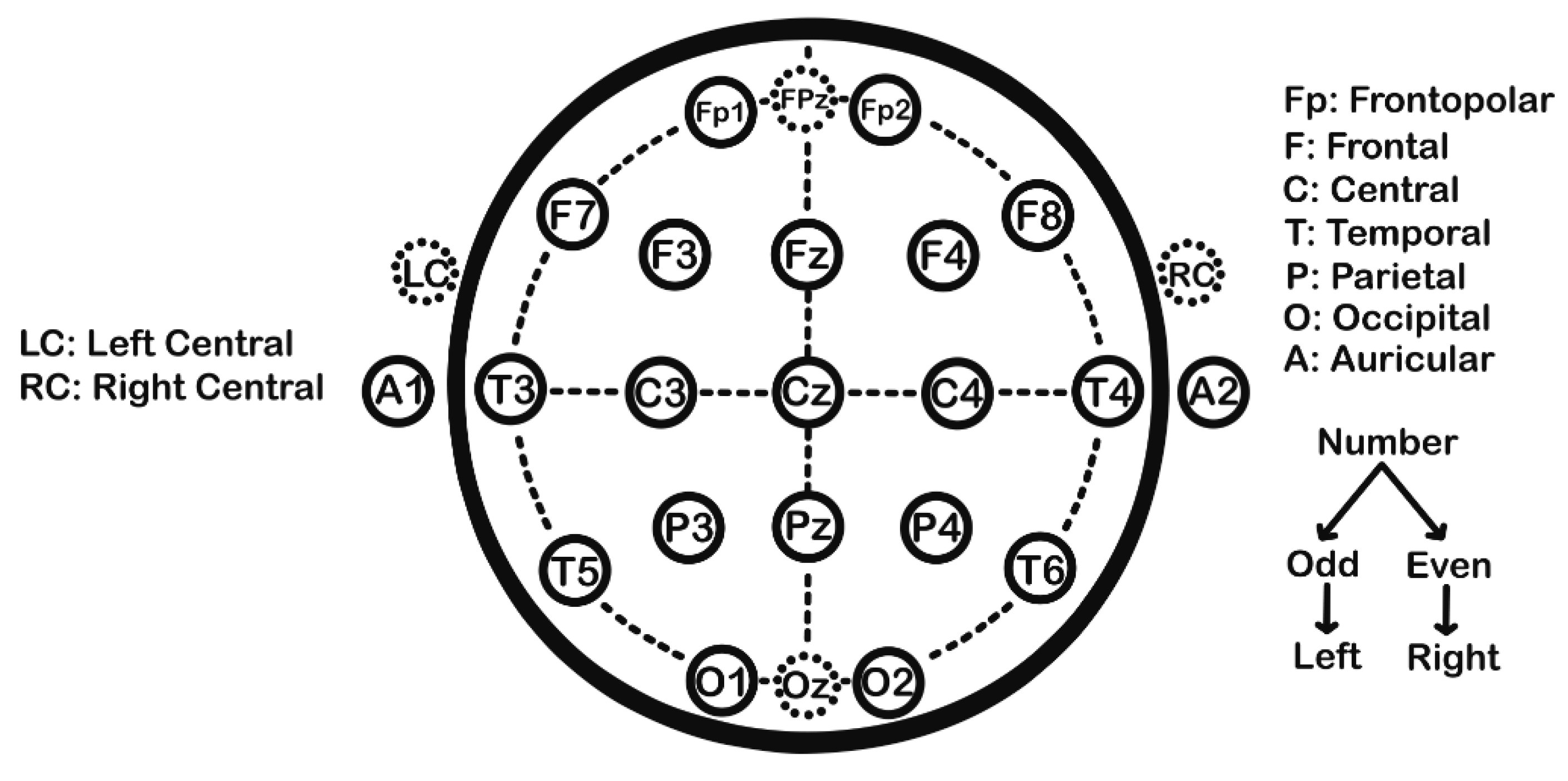
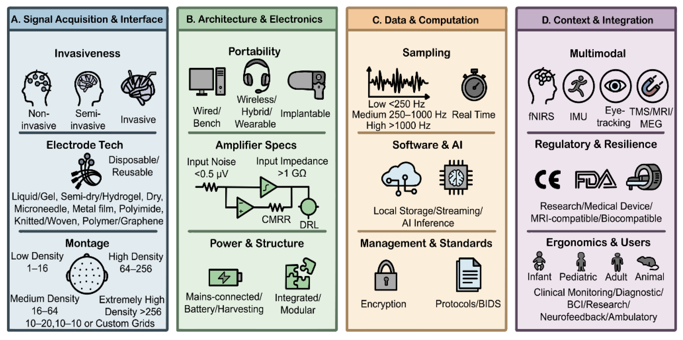
3. Recording Technique
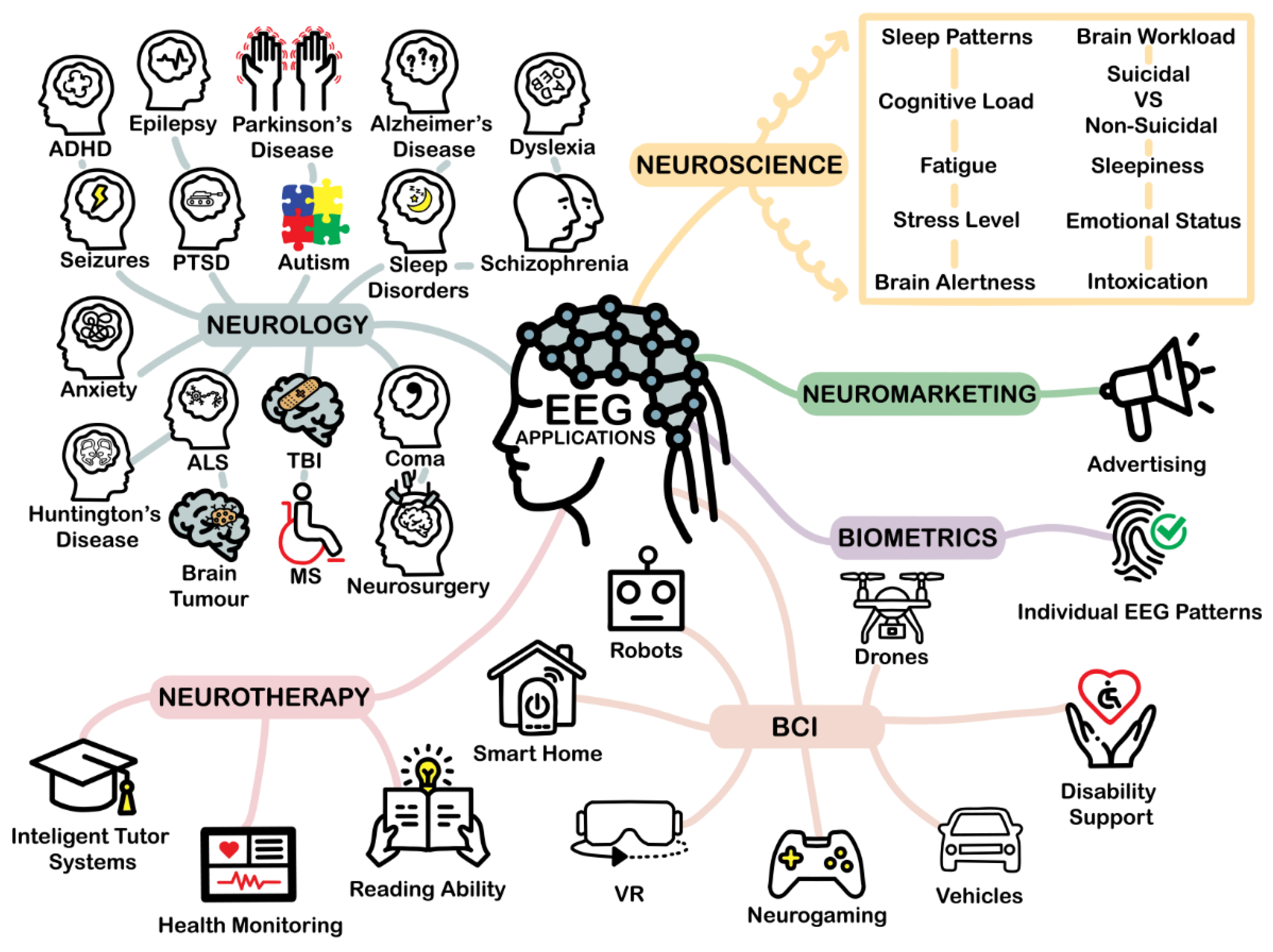
EEG technique involves recording the electrical activity of the brain through electrodes placed on the scalp, based on the principle of differential amplification, where the voltages between pairs of electrodes are amplified and displayed as waves on a digital screen. The basic components of an EEG system include the electrodes, the orientation circuits, the analog-to-digital converters (ADCs), and the processing and feedback systems. The process begins with scalp preparation, including cleansing and sometimes light skin peeling to reduce the scalp impedance below 5–10 kΩ for traditional electrode systems to improve conductivity and minimise interference [37]. The placement of electrodes follows the international 10–20 system, which ensures standardised and reproducible placement of the electrodes over brain regions (e.g., frontal, temporal, parietal). The traditional 10–20 electrode system (Figure 2) involves 19 electrode sites and two earlobe-mounted electrodes (A1/A2) that are associated with specific anatomical regions, such that 10–20% of the distance between them is used as the interval for electrode placement. The locations are named with two characters where the first character indicates the brain region (Fp = frontopolar, F = frontal, C = central, P = parietal, O = occipital, T = temporal and A = auricular), and the second character is a number (even = right, odd = left) or “z” for the central electrodes (e.g., Cz) [37,38,39,40,41,42].
EEG technology is characterised by a wide variety of design parameters and applications, which can be classified into multiple dimensions. EEG systems can be categorised based on four main axes (Figure 3): acquisition approach and interface, architecture and electronics, data and computations and context and integration [43]. In terms of signal acquisition, systems range from completely non-invasive scalp surface EEG [44], around-ear EEG for improved portability [45], and subgaleal/epicranial placement [46], to invasive techniques such as electrocorticography (ECoG) with subcutaneous arrays [47,48], stereotactic EEG (sEEG) with approved (depth) electrodes [49], and intracortical microelectrodes for research and neuroprosthetic applications [50]. The device architecture can be wired for high-reliability laboratory applications, wireless (with Bluetooth, Wi-Fi) for mobile and ambiguous studies [51], hybrid [52], wearable (consumer headsets) [53], implantable with telemetry [54], or even modular with structured electrode arrays [55]. Electrode technology covers a wide range, from the contact method: liquid/gel [56], semi-dry/hydrogel [57], dry (e.g., needle, finger) [58,59,60], microneedle electrodes [61], to construction materials such as metal films [62] and polyimide [63], knitted/woven electrodes [64], conducting polymers/graphene [65], with a distinction between active (with built-in preamplifier) and passive electrodes, as well as redeemable versus reusable. The number of channels and montage varies from low density (1–8) for basic brain-computer interfaces (BCI), medium density (16–64) for research, high density (64–256) for source detection, to extremely high density (>256) for special applications, with layouts such as the standard 10–20, 10–10, or custom grids [66,67,68].
Amplifier and signal preprocessing characteristics are critical and include input noise (e.g., <0.5 μV RMS), input impedance (e.g., >1 GΩ), common mode rejection ratio (CMRR), bandwidth and filters, dynamic 1.4, dynamic 2, dynamic bandwidth, filters, and active isolation (driven right leg) [69,70]. Temporal and spectral capabilities are determined by the sampling rate (low: <250 Hz, medium: 250–1000 Hz and high: >1000 Hz serving as approximate guidelines). Real-time latency and synchronisation methods (TTL, PTP, GPS) [71,72] are critical for closed-loop applications where the system must process data and provide feedback within milliseconds. Data management and connectivity involve local storage, data streaming, communication protocols (BLE, Wi-Fi), security, and synchronisation. The software and analysis stack includes real-time preprocessing, AI inference on the device or in the cloud, closed-loop control, and standards compliance (e.g., BIDS) [73]. Multi-modal integration is common, such as EEG + fNIRS, EEG + motion sensors (IMU), EEG + eye tracking/ECG/EGD, and synchronisation with TMS/fMRI/MEG [74,75]. Regulatory compliance and robustness determine whether a system is for research only, a medical device (Class II/III, CE, FDA), MRI compatible, or deployed for industrial use. Ergonomics are tailored to the user (infant, pediatric, adult, animal) and the duration of use. Finally, the power system can be mains-connected, battery-powered, or even energy harvesting systems, with low-power modes for extended studies, while the ecosystem can be closed (vendor-dependent) or open source/hardware [76,77,78].

4. Applications

Contemporary research is witnessing an unprecedented expansion in the application range of EEG (Figure 4) which now sufficiently provide valuable information about a wide spectrum of brain functions employed in a plethora of fields, depending on the purpose [79]. One of the most advanced areas is brain-computer interfaces (BCI), where EEG signals are used to control machines, robots, drones and prosthetic limbs, aiding people with motor disabilities [80]. Moreover, its technology is leveraged to create video games providing both entertaining and therapeutic effects. Beyond rehabilitation, it is used in neuropsychiatric diagnosis (e.g., epilepsy, Alzheimer’s disease) and in neuroscience to measure cognitive load, attention, stress and emotional state [81]. Recent research extends applications to neuroadaptive environments [82] that adjust lighting, sound or content based on the user’s brain activity, digital psychiatry [83] for detecting anxiety and depression through AI-EEG combinations [84] and neuroergonomics [85], where EEG is used in real-world or simulated environments to assess cognitive states like mental fatigue, workload and attention. This can be utilised in a new emerging research field called neuromarketing [86], where the goal is to create more effective marketing campaigns and desirable products. In the field of education, EEG is used in the evaluation of learning effort and concentration, leading to the development of intelligent and adaptive teaching systems [87]. In sports and wellness, it is utilised for neurofeedback and emotion regulation [88]. Importantly, EEG-biometric systems offer secure identification based on brain patterns [89].

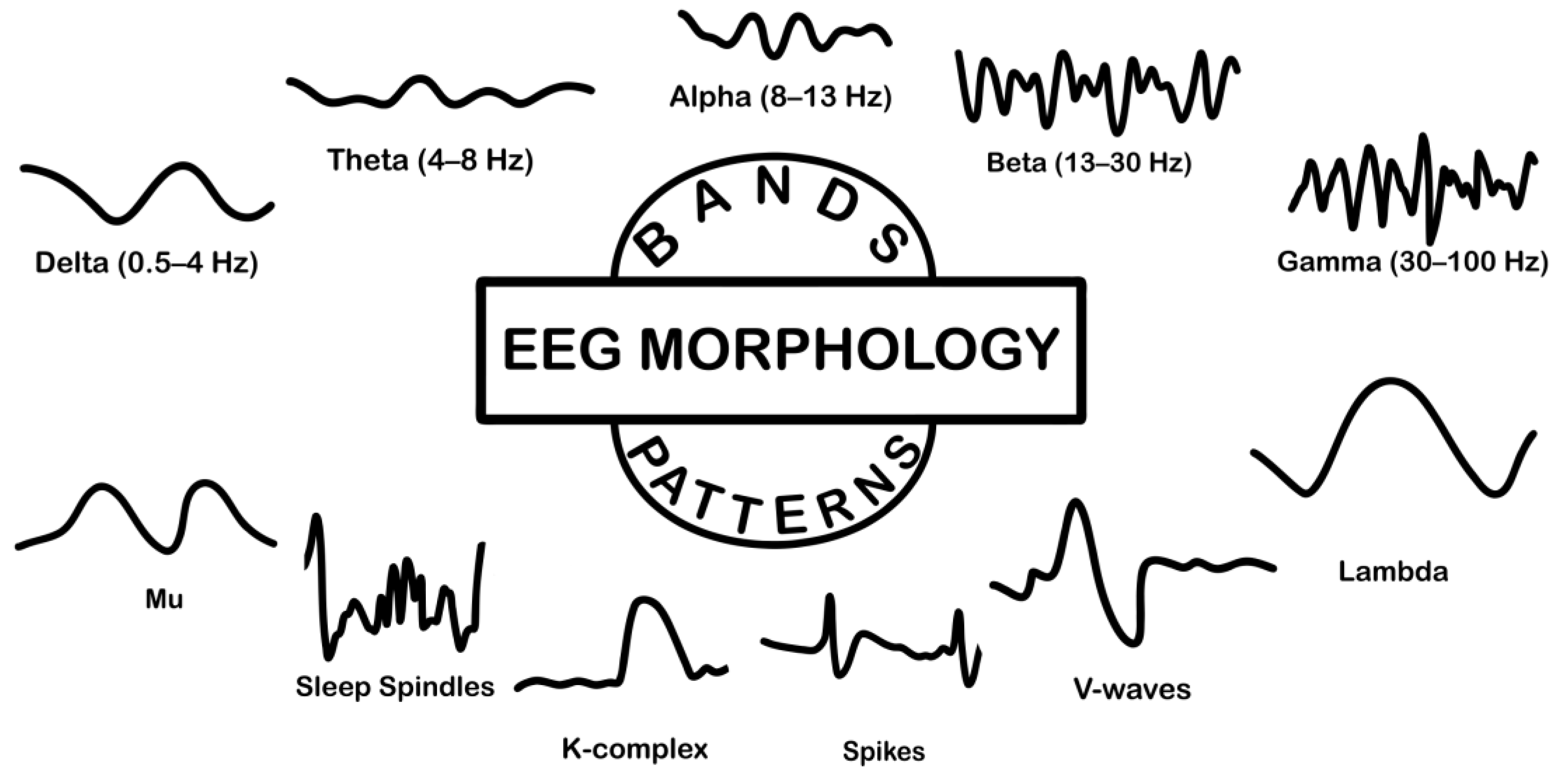
5. Basic Characteristics

EEG signals are classified by their frequency into distinct bands, each of which is associated with specific brain functions and states (Figure 5). Delta waves (0.5–4 Hz) are the predominant activity during deep sleep (stage N3) and are normal in infants, while their presence in awake adults may indicate pathology [90,91]. Theta waves (4–8 Hz) are observed during states of deep relaxation and meditation and are normal in children [92,93]. Alpha waves (8–13 Hz) predominate in the occipital region when a person is awake and calm with eyes closed and are associated with a state of calm and inner alertness [94,95]. Beta waves (13–30 Hz) are associated with active, alert thinking, concentration, and problem solving [96,97]. Gamma waves (30–100 Hz) are thought to be involved in higher cognitive functions, such as committing information to memory, perception, and integrating sensory information [98,99]. Finally, EEG frequencies above 100 Hz are not typically categorised into a standard brainwave band, but are considered part of high-frequency activity, often associated with the upper end of the gamma band and beyond. This range can be difficult to measure reliably due to low amplitude, and it can be influenced by factors like anxiety, neurostimulation, and certain neurological conditions [100,101].
In addition, EEGs show a variety of morphological patterns (Figure 5) that reflect different physiological functions or pathological conditions. The Mu (μ) rhythm occurs in the alpha frequency range (8–13 Hz) but has a characteristic arcuate shape and is recorded over the central (Rolandic) areas. In contrast to the alpha rhythm, which is suppressed by opening the eyes, the μ rhythm reacts and is suppressed during actual or even thought of movement, as it is associated with the motor cortex [102]. During sleep, several distinct patterns appear. Sleep spindles are rhythmic activity patterns in the 11–15 Hz range and are one of the defining characteristics of stage N2 (light) sleep, believed to reflect the synchronised activity of thalamo-cortical neuronal networks [103]. The K-complex is a large, high-amplitude biphasic wave that also characterises stage N2 sleep. It is a sudden delta wave, often triggered by external stimuli, and is thought to play a role in maintaining sleep by suppressing arousal [104]. Vertex waves (or V-waves) are short, sharp waves that occur in the central-frontal regions during stage N1 sleep and signal the onset of sleep [105]. In the awake state, lambda waves are transient, triangular waves that occur in the occipital region and are associated with visual exploration or saccadic eye movements, often activated during reading or watching a scene [106]. Finally, spike waves are an important EEG finding that is often associated with epileptic activity [107].
EEG is a complex, spatiotemporal signal that is often treated as a stochastic process. Although the underlying biophysical mechanisms may not be truly random, their high level of intricacy makes statistical description the usual and practical choice for quantitative analysis. EEG signals can be considered quasi-stationary over short temporal windows (on the order of a few to tens of seconds) [108]. This property is fundamental for EEG analysis, as it allows the application of classical signal processing techniques to short segments of the signal, over which it can be considered stationary and permits the estimation of instantaneous measures such as mean, variance, skewness, and kurtosis. These summary statistics and their corresponding distribution tables describe the probability of amplitude values and provide snapshots of the energy distribution; however, their estimates are strongly affected by the possible non-independence of successive samples and by the non-stationarity of the signal, so tests for normality (e.g., Kolmogorov–Smirnov) and corrections for correlation of neighboring samples must be applied with caution [109,110]. Digitisation of EEG requires sampling and smoothing/quantisation. The choice of sampling rate follows the Nyquist theorem stating that to accurately reconstruct an analog signal from its discrete sampling, the sampling frequency (sampling rate) must be at least twice the highest frequency contained in the signal. EEG analysis must be accompanied by appropriate pre-filtering to prevent aliasing, while the quantisation width (e.g., 9–11 bits) affects the signal-to-noise ratio and the fidelity of the representation [111]. Temporal correlation between samples is described by autocorrelation/coherence functions and spectral properties are projected via the power spectral density, which is the Fourier transform of the autocorrelation. Techniques such as periodogram/FFT and smoothing or ensemble-averaging modes are used for reliable spectrum estimates, while spectral moments and parameters such as Hjorth indices summarise morphological features of the spectrum [112]. When the distribution is non-Gaussian, higher-order analysis (e.g., bispectrum/bicoherence) reveals nonlinear correlations and spectral phase coupling between harmonic components [113,114]. Alternatively, interval or period analysis based on zero-crossing machines, measurement of intervals between peaks or half-waves, and interval-amplitude diagrams offers a simple but powerful temporal description of wave structure and is mathematically related to spectral moments and zero-crossing rates (N0, N1, N2), although it is sensitive to high-frequency noise (hysteresis/dead-band is commonly introduced to avoid spurious crossings) and tends to overestimate fast components while underestimating rare long periods [115]. In summary, the comprehensive description of EEG for research combines statistical snapshots (distribution shapes and moments), temporal relationships (auto-/intercorrelation), and spectral representations (PSD, high-order spectra), complementing -where necessary- parametric approaches (e.g., AR models) or pattern detection methods for feature extraction [116].

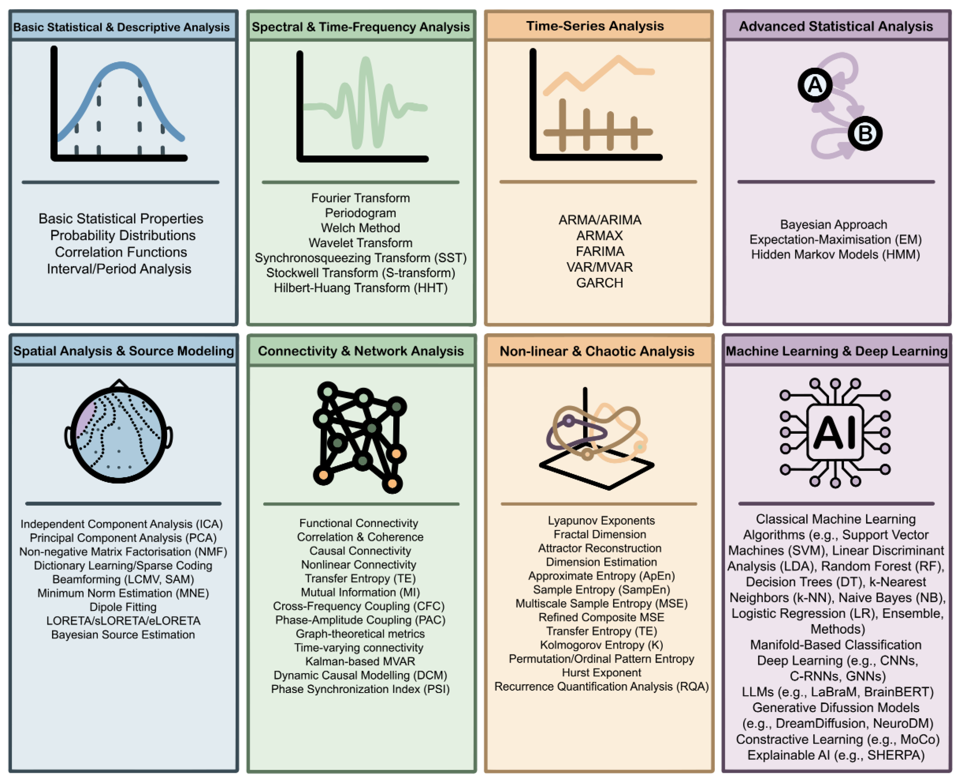
6. Methods for EEG Processing

6.1. Basic Statistical & Descriptive Analysis

Basic statistical and descriptive methods are the cornerstone of quantitative analysis of EEG signals, as they allow an initial understanding of their shape, variability and statistical behavior. EEG, as a stochastic and nonlinear signal, exhibits fluctuations that reflect the dynamic interaction of large populations of neurons. As mentioned previously, descriptive parameters, such as mean, variance, standard deviation, skewness and kurtosis, are handy tools to get key insights into the statistical properties of the signal [117,118]. At the same time, the investigation of the probability distributions of the EEG provides information on the nature and nonlinearity of the underlying processes and it is the deciding factor in the selection of appropriate statistical tests or models.
The correct choice of sampling frequency, according to the Nyquist theorem, and the use of appropriate anti-aliasing filters are vital for the prevention of distortions as well as the loss of information, while the analysis in bits governs the accuracy of the recording. The autocorrelation and cross-correlation functions can be used to estimate temporal dependencies and delays between channels, providing a first takeaway of synchronisation or functional correlation [119,120]. Finally, methods such as interval or period analysis pave the way for the study of wave periodicity, utilising techniques such as calculating zero-crossings or half-wave intervals to extract simple but insightful temporal features [121,122]. Overall, basic statistical and descriptive methods constitute a necessary first level of analysis, which not only provides an initial overview of the data, but also guides the selection of more complex spectral, parametric or nonlinear approaches.

6.2. Spectral & Time-Frequency Analysis

There are a lot of transformations that reveal the energy structure of the EEG in terms of frequency. The Continuous Time Fourier Transform (CTFT) transforms a time signal into a frequency signal, representing it as a sum of sine and cosine functions [123]. For a continuous signal x ( t ) , it is defined by Equation (8) where f is the frequency spanning from 0 Hz to half the Nyquist frequency and j the imaginary unit.
    F f = x t e j 2 π f t d t ,
According to Fourier analysis, any physical signal can be decomposed into discrete frequencies or a continuous frequency spectrum. The statistical average of the signal is called EEG spectrum and allows the analysis of the signal in the frequency domain, showing the contribution of each frequency to the signal. EEG signals are discrete due to digitisation since the sampling process converts the original analog signal into a sequence of discrete time instants and quantisation converts the actual voltages into discrete numerical values. Since the input is a sequence of numbers, the mathematically appropriate tool for its analysis in the frequency domain is the Discrete Fourier Transform (DFT) (9) which acts on a discrete-time signal consisting of N samples. The index of the frequency component calculated ( k ) corresponds to a specific frequency f k = k × F s N , where F s is the sampling frequency [124].
  F f = n = 0 N 1 x n e j 2 π k n N ,
DFT is implemented via the Fast Fourier Transform (FFT) algorithm which takes advantage of the symmetries and periodicities of the exponential term to break the calculation into smaller, repeated steps, reducing the complexity from O ( N 2 ) to O ( N log 2 N ) [125]. The Short-Time Fourier Transform (SFFT) calculation (10) procedure is as follows: 1) The signal is divided into segments and a sliding window is applied ( m is the window shift index in time). 2) Each segment is multiplied by a window function w [ n ] [126]. 3) The DFT (via FFT) is computed on each windowed segment, giving the spectral coefficients for each position. Small windows offer good time but poor frequency resolution, while large windows do the opposite, a fact that expresses the Heisenberg uncertainty limit. Although simple and flexible, the STFT does not automatically adapt to changes in the frequency structure of the signal, and for this reason it is often combined with other techniques (such as multitaper or wavelets) for improved statistical accuracy and spectral leakage reduction.
STFT x t m ,   ω = n = x n w n m e j ω n ,
This transformation allows us to calculate the power spectrum and quantify the energy in the classic brain waves (delta, theta, alpha, beta, gamma), providing fundamental information about brain function. By applying the Fourier transform we can obtain the power spectral density (PSD), which is directly related to functional activity and cognitive states [127]. It has been used as a basic tool for extracting spectral features by detecting frequencies associated with physiological states such as sleep [128], mental load [129] or pathological states such as epilepsy [130]. Nevertheless, the FFT assumes that the signal is stationary within the analysis window. This results in weaknesses in detecting transient phenomena. For example, it cannot detect short signal changes well (such as the characteristic “spikes” in epileptic seizures). It also requires a relatively long signal length to provide reliable spectral estimation, as very short segments have low frequency resolution and cause spectral leakage due to the window boundaries. The FFT is also sensitive to noise.
In contrast to the FFT, which can be used to obtain the amplitude and phase, the Periodogram is a simpler method for a statistical estimation of the spectrum. It is utilised to obtain information only about how the power (energy) of the signal is distributed in the frequency spectrum. It is the basic non-parametric estimation of the PSD and it is calculated from the square of the magnitude of the DFT of the signal, normalised with the sample length (11) [131]. This facilitates the comparison of the power spectrum of different signals, or of the same signal under different conditions, the identification of periodicities as well as the frequency with the maximum contribution to the total power of the signal. The periodogram is statistically inconsistent since the variance of the estimate does not decrease with increasing number of samples, making it sensitive to noise [132]. Because of this variability, smoothing techniques were developed to achieve a more stable estimate, a development that led to the Welch method. The Welch method takes many “statistical samples” (from overlapping segments) and combines them to give a much more reliable picture. The original signal x [ n ] of length N is divided into K overlapping segments. Each segment i has length L . The i -th segment is: x i m = x m + i × D ,   m = 0 ,   1 , , L 1 , where D is the number of offset samples between two consecutive segments (if the overlap is 50%, then D = L / 2 ). The total number of segments is K = N L D + 1 . A window function w n   is applied to each segment, so the window section is u i m = x i m × w m . The periodogram is calculated for each windowed section (12) and the final PSD estimate from the average of the individual periodograms (13) [133].
P f = 1 N n = 0 N 1 x n e j 2 π k n N 2 ,
P x x i f = 1 L × U n = 0 L 1 u i m × e j 2 π f m L 2 ,
P x x W e l c h f = 1 K i = 0 K 1 1 L × U m = 0 N 1 u i m × e j 2 π f m L 2 ,
Unlike the Welch method, which relies on dividing the signal into overlapping segments and applying a single window to control spectral leakage, the Multitaper method applies multiple optimal mathematical windows (Slepian Tapers), which are designed to maximise the concentration of spectral information within a predefined frequency bandwidth, while minimising leakage outside it [134]. Thus, eliminating the need for subjective window selection and segmentation. This fundamental difference offers a statistically superior estimate of the power spectrum, with minimised variance and minimal leakage at the same time, making it particularly robust for the analysis of short and dynamically changing EEG, where the Welch method can introduce significant bias or miss critical temporal details.
The Wavelet Transform is a fundamental tool in the study of non-stationary signals that overcomes the limitations of the classical Fourier. The mathematical core of the method is based on the concept of the mother wavelet, a function of short duration and zero mean, which resembles a small wave or pulse. The central idea is the following: instead of decomposing the signal into sinusoidal functions of infinite duration, the wavelet transform uses the mother wavelet, which shifts and scales in time, to investigate the signal at different time scales. The significant difference from the STFT is that instead of using a fixed-size window, the window size is adjustable. For high frequencies, the window is narrow, providing high temporal resolution, while for low frequencies, the window is widened, providing high frequency resolution. The Continuous Wavelet Transform (CWT) of a signal x ( t ) is defined according to Equation (14) as the inner product of the signal with a shifted and scaled version of the parent wavelet ψ ( t ) (e.g., Morlet, Mexican Hat, Daubechies), where a is the scale factor which controls the “stretching” of the wavelet, b   the translation factor which handles the temporal position of the wavelet along the signal and ψ * denotes the complex conjugate.
W a , b = 1 a + x t ψ * t b a d t ,
CWT calculates the coefficients W a , b for a continuous range of scales and time shifts, creating a two-dimensional power map (scalogram) that illustrates at which times and frequencies EEG activity is increased. The Discrete Wavelet Transform (DWT) is based on the sampling of the scale and shift parameters at discrete values, usually a = 2 j and b = k × 2 j , where j , k Z . The DWT analyses the signal through binary multiresolution analysis (MRA), separating the signal into two main parts at each level: low frequencies (approximation coefficients), representing the general form of the signal and high frequencies (detail coefficients), representing the details and transient features. The process is implemented through low-pass and high-pass filters, which are applied iteratively to successive decomposition levels [135,136,137]. The inverse process (inverse DWT) allows the reconstruction of the signal without loss of information. Simply put, the CWT acts like a “magnifying lens” that scans each moment in time at all frequencies, while the DWT “breaks” the signal into structural levels, revealing the content of the EEG in an economical but complete way. Wavelet Packet Decomposition (WPD) is a generalisation of the DWT. While in DWT for all subsequent decomposition levels, only the low-frequency approximation component is further split into new approximation and detail components, in WPD, both the low-frequency approximation and the high-frequency detail components are recursively decomposed in subsequent levels. In this way, WPD offers a more uniform and flexible analysis of the entire frequency spectrum, making it extremely useful for EEG signals that contain information at multiple, non-hierarchically organised frequencies [138]. Wavelet Transform has been used in various ways, including feature extraction [139], EEG signal denoising [140], seizure [141] and Event Related Potentials (ERPs) detection [142].
The Synchrosqueezing Transform (SST) is an improved and re-distributed version of the Wavelet Transform (WT), designed to provide better spectral clarity and detection of time-varying frequencies. Initially, CWT is calculated (14) and then the instantaneous frequency is computed (15). Then, the wavelet coefficients are “squeezed”, redistributing the energy from the region ( a , b ) to the frequency ω , through the kernel (16), where δ is Dirac delta function [143].
ω a ,   b = i t W a , b W a , b ,
T ω , b = W a , b δ ω ω a , b d a ,
SST refines the wavelet scalogram moving the energy from areas of ambiguity to the correct frequencies, achieving highly accurate time-frequency representations [144,145]. Stockwell Transform (S-transform) (17) uses a frequency-changing window, like wavelet transform, but in addition, preserves the phase. It uses the Gaussian window function, which depends on the frequency and the time shift parameter τ , which determines the center of the Gaussian window in time [146].
S τ , f = + x t f 2 π e τ t 2 f 2 2 e i 2 π f t d t ,
Stockwell Transform (S-transform) analyses the signal as “an orchestra of oscillations” arising from the EEG itself, without imposing an external basis. It consists of two stages: (a) Empirical Mode Decomposition (EMD) decomposes the signal x ( t ) into a finite number of Intrinsic Mode Functions (IMFs) (18), where each c i t is an IMF and r n t is the residual (trend). (b) Then, each IMF is subjected to a Hilbert Transform (19) ( P . V . is the Cauchy Principal Value which ensures that the integral converges) and the analytical representation is defined (20) where a i t   is the instantaneous amplitude and φ i t is the instantaneous phase [147,148].
x t = i = 1 n c i t + r n t ,
c ~ i t = 1 π P . V . + c i τ t τ d τ ,
z i t = c i t + j c ~ i t = a i t e j φ i t ,

6.3. Time-Series Analysis

EEG signal is a time-series as it captures measurements of the brain’s electrical activity over a consistent interval of time. Thus, time-series methods can be applied. The Prony method is an ancestor of parametric autoregressive models, using exponential fitting to the signal (21), where A i is the amplitude and s i = α i + j ω i is the complex frequency [149,150].
x t = i = 1 N A i e s i t ,
The method fits a sum of damped exponential functions and is useful for the estimation of dominant frequency components, analysis of damped oscillations and modeling of transient episodes. In modern applications, it has been extended to Matrix Prony and Subspace Prony [151], which utilise algebraic and eigenspace (subspace) techniques to estimate exponential components in multichannel EEG signals, allowing more stable and accurate identification of dominant oscillatory modes and temporally consistent spectral analysis even in highly noisy data.
A signal x t can be described by an Autoregressive (AR) model as a linear combination of its p previous values (22), where a i is the autoregressive coefficient and ε t is white noise. Hence the AR model predicts the current value based on the memory of the signal. In a Moving Average (MA) model the signal depends on the current and past errors (23), where b i corresponds to a noise filter. The MA smooths out the stochastic variability, capturing transient or random fluctuations. Autoregressive Moving Average (ARMA) combines the previous two (24) and offers a balance between memory and random component, which is ideal for EEG that exhibits both internal dynamics and noisy effects. Parameter estimation is executed with methods such as Yule-Walker, Levinson-Durbin, or Burg’s algorithm [152,153,154]. Extending ARMA by introducing an integration term for non-stationarity, we obtain the Autoregressive Integrated Moving Average (ARIMA) (25), where B is the lag operator and d is the degree of integration. Thus, ARIMA(p,d,q) can describe EEG series with long-term variations or trends, while preserving local dynamics [155]. In Autoregressive Moving Average with Exogenous Inputs (ARMAX) models, external variables u t are introduced that do not belong to the system itself but affect the behavior of the time series, such as sensory stimuli or experimental conditions that affect the EEG during recording (26). In practice, it allows the modeling of EEG with stimuli (e.g., sensory input, task events), combining temporal memory, stochasticity and external influence [156]. Fractional ARIMA (FARIMA or ARFIMA) generalises ARIMA by allowing fractional integration d R  (27). This facilitates the capture o long-range dependence or memory effects in EEG. This means that current samples are influenced not only by recent, but also by incredibly old events [157]. Vector Autoregressive (VAR) models extend AR to multivariate time series (28), where x t is a vector of EEG channels, A i is the coefficient matrix, and ε t is an error vector. The basic idea is that each channel can influence and be influenced by the others, thus allowing the analysis of interdependencies and causality between brain regions [158]. Multivariate VAR (MVAR) extensions allow the calculation of the Granger causality which estimates whether the activity of one channel can predict the future behavior of another, the Directed Transfer Function (DTF) and the Partial Directed Coherence (PDC) which are based on the spectral representation of the MVAR model and support the estimation of frequency-dependent directionality, while their time-varying extensions capture how these causal connections change dynamically during cognitive processes or states [159,160,161]. Volatility, how the noise or energy of the signal changes over time, can be modeled with the Generalised Autoregressive Conditional Heteroskedasticity (GARCH) model. The central idea of GARCH(p, q) is that the variance of the noise depends on previous values of the variance and the errors. For a time-series x t , σ t 2   is the conditional variance, which evolves according to Equation (29) [162]. Choosing the optimal p, q order of a parametric model is critical to the accuracy and stability of the model. The most common criteria are the Akaike Information Criterion (AIC) and the Bayesian Information Criterion (BIC) [163]. All these methods have been used for instance in dealing with artifacts [164], the prediction of epileptic seizures [165], the diagnosis of autism [166], and the real-time monitoring of the effects of drugs (such as anesthetics) [167].
x t = i = 1 p a i x t i + ε t ,
x t = i = 0 q b i ε t i ,
x t = i = 1 p a i x t i + j = 0 q b j ε t j ,
d x t = ( 1 B ) d x t ,
x t = i = 1 p a i x t i + j = 0 q b j ε t j + k = 1 r c k u t k ,
( 1 B ) d x t = ε t ,   w h e r e ( 1 B ) d = k = 0 Γ k d Γ d Γ k + 1 B k ,
x t = i = 1 p A i x t i + ε t ,
σ t 2 = α 0 + i = 1 q α i ε t i 2 + j = 1 p β j σ t j 2 ,

6.4. Advanced Statistical Analysis

The goal of advanced statistical and probabilistic methods is not only to describe the signal, but also to estimate the possible generating processes behind it. Bayesian approach is based on Bayes’ Theorem (30) [168].
P θ D = P D θ P θ P D ,
The logic is that we combine prior knowledge (priors) with observed data to get updated estimates (posterior estimates). Bayesian approach is instrumental to Bayesian source localisation, which estimates the most likely distribution of brain sources that produce the observed signal, hierarchical bayesian models, which estimates connectivity by integrating information between subjects and uncertainty quantification, which calculates probabilities for the reliability of each parameter [169]. Another useful tool is the Expectation-Maximisation (EM) algorithm which is an iterative optimisation approach used when data contains latent (unobservable) variables. The objective is to maximise the likelihood P ( X θ ) based on the available data X and the algorithm alternates between two stages: E-step calculates the expected value of the latent variables (Expectation) and M-step updates the parameters by maximising the expected likelihood (Maximisation) [170,171]. EM is exploited in gaussian mixtures for clustering EEG states as well as in Hidden Markov Models (HMM) and Dynamic Causal Modelling (DCM) for parametric estimation. HMMs assume that there is a latent sequence of states S t that produces the observed data X t and the probability of the entire sequence is calculated by Equation (31) [172].
P X , S = P S 1 t P S t S t 1 P X t S t ,
This way, the EEG is considered as an alternation of latent “brain states”, which are not directly observed, but leave an imprint on the EEG waves. The estimation of the parameters is usually done with the EM algorithm and these models have been used in the detection of brain states (e.g., sleep, attention, judgment), brain-state decoding and dynamic functional connectivity and event segmentation in cognitive experiments [173]. DCM is a Bayesian state-space model that describes how brain regions interact causally. The system is described by differential Equation (32), where x is the internal brain states, u is the external stimuli and θ is the connection strengths. The parameters are estimated via variational Bayes (VB), which approximates the posterior distribution of connections [174]. DCM does not simply describe correlations, but how one region causes the response of another. Thus, it is a causal generative model. It is useful in the analysis of directional connectivity (effective connectivity) [175].
x ˙ = f x , u , θ ,

6.5. Spatial Analysis & Source Modeling

Spatial analysis and source modeling includes methods for estimating EEG brain sources (inverse problem). Independent Component Analysis (ICA) is based on the model (33), where the observed EEG signal x is a linear mixture of independent sources s , through a mixing matrix A .
x = A × s ,
The method aims to estimate A 1 , maximising the statistical independence of the components (e.g., through maximising non-Gaussianity or minimising mutual information). This technique is used in EEG denoising (EOG/EMG subtraction), detection of independent rhythms, and functional source analysis (EEG-fMRI integration) [176]. Joint ICA (EEG-fMRI) is applied to unified datasets X = [ X E E G , X f M R I ] , where the aim is to find common independent factors that explain both modalities simultaneously. Instead of separating only EEG components, it finds common spatiotemporal factors that explain both the dynamics of the EEG and the spatial distribution of the fMRI. It has been used in combined spatiotemporal interpretation of functional brain activity (neurovascular coupling) [177]. Independent Vector Analysis (IVA) extends ICA to multiple datasets (34) where each s k is independent of the others.
x k = A k s k ,     k = 1 , , K ,
The goal is to estimate A k that preserve internal interdependence and external independence. It has been utilized in group-level EEG analysis, multimodal analysis (EEG-MEG) and comparative EEG studies in populations [178,179]. Principal Component Analysis (PCA) finds orthogonal components that maximise the variance of the data (35).
X = U Σ V T ,
The principal components are the columns of V , and the eigenvalues of X T X give the contribution of each component. This method reduces the dimension of the EEG to a few axes that describe the largest variation (energy) of the signal. It has been used in pre-processing for ICA, data compression, EEG power factor analysis and pattern classification [180].
Non-Negative Factorisation (NMF) assumes that the data X can be approximated as a sum of positive bases W that are time activated by H  (36). Practically, this means we look for repeating spatial/temporal patterns that add up to form the signal. This is useful for isolating alpha/β patterns and artefacts [181,182]. In Sparse Coding or Dictionary Learning we assume that each instance of the signal is written as a linear combination of some columns of a dictionary D , with sparse coefficients α  (37) [183,184]. In other words, we have a “dictionary of waveforms” and at any given time a few of them are activated. EMD mentioned before decomposes the signal into intrinsic oscillations (IMFs) plus a residual (38). It peels the signal to isolate the natural, local time-varying frequencies, suitable for transient/nonstationary features. In the inverse source localisation problem, the linear model x   =   L j   +   n is used [185]. Beamformers construct spatial filters w that maximise the gain at the location of interest and minimise the power elsewhere, the formulation and closed-form solution are given in (39) [186,187]. The Minimum-Norm Estimate (MNE) favours the solution with the lowest total energy and is written as regularised least-squares (40), so when several scenarios explain the data, we choose the most parsimonious explanation [188]. Variants such as LORETA/sLORETA/eLORETA introduce spatial smoothness terms (matrix R ) in the normalised problem for smoother and more reliable source allocations (41) [189]. Dipole fitting is expressed as a nonlinear optimisation for fitting a few dipoles ( θ , q ) that explain the signal and formulated in (42) [190,191]. These methodologies are chosen or combined depending on the objective (e.g., beamformer for targeted spatial isolation, MNE/LORETA for distributed evoked maps, dipole fitting for focal sources), while decomposition techniques (NMF, dictionary learning, EMD) are often used as pre-processing or to extract features.
min W , H 0 X W H F 2 ,
min D , A X DA F 2 + λ A 1 ,   s . t .   d k 2   1 k ,
x t = k = 1 K I M F k t + r t ,
min w w R w ,     s . t . w l = 1 w = R 1 l l R 1 l ,
j ^ = a r g min j x L j 2 2 + λ j 2 2 j ^ = ( L L + λ I ) 1 L x ,
j ^ = ( L L + λ R ) 1 L x ,
min θ , q x L θ q 2 2 ,

6.6. Connectivity & Network Analysis

Another domain of EEG analysis is the study of functional and causal relationships between brain regions based on temporal, spectral and probabilistic correlations. Functional connectivity measures statistical correlation or coherence between pairs of signals: Pearson satisfies the need for linear correlation between two time series (43), while Coherence expresses the frequency-dependent linear relationship through spectral densities (44) [192]. In practice, high r or coherence values in a specific band indicate possible involvement in common cognitive processes and are used in studies of hemispheric cooperation, sleep, and pathologies such as epilepsy [193]. Causal connectivity is based on MVAR models that predict the present from the past; in Granger’s formulation, if the predictive power of one signal is improved by adding the past terms of another, we consider that Granger causality exists (45). Spectral extensions of this framework give the frequency transfer function H ( f )  (46) and directivity measures such as the DTF (47) and PDC (48) mentioned before, which represent the flow of information per frequency; these are useful for identifying information flow in sensory networks and pathological conditions [194].
r x y = E x μ x y μ y σ x σ y ,
C x y f = S x y f 2 S x x f S y y f ,
x t = k = 1 p A x x k x t k + k = 1 p A x y k y t k + e t ,
H ( f ) = ( I k = 1 p A k e i 2 π f k ) 1 ,
D T F i j f = H i j f 2 k H i k f 2 ,
P D C i j f = A i j f k A k j f 2 ,
Nonlinear connectivity analysis includes metrics such as Transfer Entropy (TE) [195], which measures the directional nonlinear information from Y to X (49), and Mutual Information (MI) [196], which measures the general mutual dependence between two variables (50); the intuition here is that these metrics detect relationships that are not constrained by linearity or Gaussian assumptions and are therefore applicable to complex cognitive processes, judgments, and consciousness studies.
T E Y X = p x t + 1 , x t , y t log p x t + 1 x t , y t p x t + 1 x t ,
M I X , Y = x , y p x , y log p x , y p x p y ,
Phase methods focus on phase synchronisation: Phase-Locking Value (PLV) measures the stability of the phase difference (51), Phase-Lag Index (PLI) excludes zero phase lags to reduce the effect of volume conduction (52), while weighted-PLI (53) and Amplitude Envelope Correlation (AEC) (54) provide variants that emphasise reliable, non-zero phase contributions or amplitude envelope correlation; these measures are widely used to study phase locking in attention, perception, neurofeedback, and epilepsy. Cross-Frequency Coupling (CFC), and especially Phase-Amplitude Coupling (PAC), examines whether the phase of a low frequency modulates the amplitude of a higher one; this can be measured simply as phase-amplitude correlation or with the Modulation Index (Tort) based on Kullback-Leibler divergence (55), and serves to highlight hierarchical neural interactions (e.g., memory, attention) [197,198,199].
P L V = 1 N n = 1 N e i ϕ x n ϕ y n ,
P L I = sign sin ϕ x ϕ y ,
w P L I = E Im S x y E Im S x y ,
A E C = corr e n v x t , e n v y t ,
P A C corr p h a s e low t , a m p high t , M I = D K L P U log N ,
Symbolising connectivity as a graph G(V,E) allows the calculation of indicator graphs such as modularity Q  (56), global efficiency (57), clustering coefficient (58), and centrality metrics, which quantify the organisation, efficiency, and roles of nodes in the network. Such indices are applied in resting-state studies and in diseases such as Alzheimer’s [200]. Since connectivity varies over time, time-varying approaches are applied: sliding windows for time-local estimates or Kalman-based/recursive MVAR models [201] where the parameters A t change over time and are estimated using Bayesian or recursive filters (59); these are crucial for studying dynamic FC, microstates, and task-related changes. DCM model mentioned previously approaches causality with biophysically parameterised state-space models (60) and Bayesian inversion to estimate the effect of experimental factors on connections; DCM allows comparison of causal structure hypotheses and is widely used in SPM for EEG/MEG [202]. Finally, the Phase Synchronisation Index (PSI) generally measures the stability of the phase difference (61) and is used to evaluate synchronisation in sensory, motor, and cognitive processes [203]. In all of the above approaches, the choice of the appropriate metric depends on the background of the hypothesis (linear vs. nonlinear, statistical vs. causal), sensitivity to volume conduction, desired spatial/temporal resolution, and the semantics of the study; practical factors such as spectral density estimation, noise model, normalisation, and correct estimation of hyperparameters are critical for reliable conclusions.
Q = 1 2 m i , j A i j k i k j 2 m δ c i , c j ,
E g l o b = 1 N N 1 i j 1 d i j ,
C i = 2 T i k i k i 1 ,
x t = A t x t 1 + w t ,
x ˙ = A x + B u + C ,
P S I = 1 N n = 1 N e i ϕ x n ϕ y n ,

6.7. Nonlinear & Chaotic Analysis

EEG activity is an extremely complex and nonlinear signal that reflects the collective action of large neural populations. Brain dynamics are often characterised by nonlinear interactions, transient states, and chaotic behavior, which makes the use of purely linear models inadequate for their description [204]. For this reason, a wide range of nonlinear and chaotic analysis methods have been developed, which allow the investigation of the stability, complexity, and predictability of EEG time-series, offering a deeper understanding of the underlying neural dynamics. One of the fundamental measures in chaos theory is the Lyapunov exponents, which describe the average rate of divergence of two neighboring trajectories in phase space. If two initial states differ by d x ( 0 ) , then the Lyapunov exponent is defined as the logarithm of the ratio of the final to the initial distance, divided by time (62):
λ = lim t 1 t ln δ x t δ x 0 ,
Positive values of λ indicate sensitivity to initial conditions and therefore chaotic behavior. In EEG analysis, the presence of positive Lyapunov exponents has been linked to unstable and chaotic neural states, such as in epileptic seizures, while negative or zero values correspond to stable or periodic states, such as sleep or anesthesia [205,206]. Fractal dimension (D) is another fundamental measure of complexity, as it expresses how the detail of a signal changes with the scale of observation. Using the box-counting approach, this dimension is defined as the limit of the ratio of the logarithms of the number of squares N ( ϵ ) required to cover the signal trajectory and their inverse size (63).
D = lim ϵ 0 log N ϵ log 1 ϵ ,
High D   values correspond to more complex EEG signals, which have been observed during cognitive processes or in pathological conditions such as epilepsy. To investigate the dynamic structure of the EEG, reconstruction of the attractor in phase space is often used, according to Takens’ theorem. Each point of the signal can be represented as a state vector x t through the delay τ and the embedding dimension m, as shown in Equation (64). The geometry of the reconstructed tractor can be described by the correlation dimension ( D ) , defined by the correlation function C ( r ) in Equation (65).
x t = x t , x t + τ , , x t + m 1 τ ,
C r = 2 N N 1 i < j H r x i x j , D 2 = dln C r dln r ,
The existence of a low-dimensional attractor ( D   <   5 ) is indicative of chaotic but limited dynamics, which has been observed in epileptic seizures and cognitive transitions [207,208,209]. Approximate entropy (ApEn) introduces a statistical measure of signal regularity. It is defined as the difference between the probability that similar patterns of length m remain similar when extended by one dimension, as given in Equation (66). Low ApEn values indicate predictable signals, while high values indicate greater complexity. Sample Entropy (SampEn) improves ApEn by excluding self-correlations and is defined as the negative logarithm of the ratio of probabilities A and B of two similar patterns of length m + 1 and   m  (67). SampEn is less biased and more reliable in short EEG sequences, which is why it is used in studies of sleep, consciousness, and cognitive load. Multiscale Sample Entropy (MSE) extends SampEn by calculating entropy at different time levels through “coarse-graining” of the signal. Each new sequence is obtained as the average of the values within windows of length τ according to Equation (68). In this way, MSE provides a profile of complexity at multiple time scales, while the Refined Composite MSE (RCMSE) version offers improved stability for short EEG time-series [210]. Kolmogorov entropy (K) links chaos theory with information theory, expressing the rate at which new information is generated in a dynamic system. It is defined as the sum of all positive Lyapunov exponents, as shown in Equation (69). High K   values correspond to increased chaos and rapid loss of predictability, characteristics that have been observed in EEG states of increased neural excitation. Permutation entropy (PE) offers a quick and efficient assessment of EEG complexity. It converts the time series into permutation sequences and calculates the Shannon entropy of their probabilities, as given in Equation (70). This measure is particularly robust to noise and has been used extensively in applications such as seizure detection and anesthesia monitoring. TE (49) mentioned before measures the nonlinear, directed flow of information between two time series and is defined as the conditional information difference between probability distributions. Unlike Granger’s Linear Causality, TE does not assume linearity or normality and has been widely used to study the effective connectivity of the brain [211,212].
A p E n m , r , N = ϕ m r ϕ m + 1 r ,
S a m p E n m , r , N = ln A B ,
y j τ = 1 τ i = j 1 τ + 1 j τ x i ,
K = λ i > 0 λ i ,
P E = i = 1 n ! p i ln p i ,
Another fundamental measure is the Hurst exponent (H), which quantifies the long-term dependence and self-similarity of the signal. The relationship between the R / S ratio and the sample size N follows Equation (71). H   values greater than 0.5 indicate persistent behavior, while values less than 0.5 correspond to mean-reverting processes. The measurement of H has been applied in the analysis of fatigue, aging, and cognitive levels [213,214]. Finally, Recurrence Quantification Analysis (RQA) is based on the creation of a recurrence plot, i.e., a table that records when the system’s trajectory returns to previous states. This table is defined as (72) where Θ is the Heaviside function and ϵ is the proximity radius. This table yields indices such as the repetition rate, determinism, and stationarity, which reveal transitions between different brain states [215,216,217]. Overall, the above nonlinear and chaotic methods provide a multidimensional approach to the study of brain activity.
R S N H ,
R i j = Θ ϵ x i x j ,

6.8. Machine Learning & Deep Learning

The analysis of EEG signals has been reshaped in the last half-decade. Τhe manual feature engineering that defined the late 20th century paved the way for sophisticated data-driven approaches, more suitable for the dynamic human brain signals [218]. A plethora of ML algorithms have been used, and the choice of classifier depends heavily on the dataset size and the requirement for interpretability. Support Vector Machines (SVM) are the most robust classifier for “small data” regimes, which characterises many BCI pilot studies (where N < 20 subjects). SVMs map input vectors into a high-dimensional space using a kernel function (e.g., Radial Basis Function) to find the optimal hyperplane separating two classes (e.g., “Left Hand Movement” vs. “Right Hand Movement”). Linear Discriminant Analysis (LDA) is the standard for Brain-Computer Interfaces (BCI), particularly in P300 speller paradigms. It assumes that each class follows a Gaussian distribution with a shared covariance matrix. It is less powerful than nonlinear classifiers but its simplicity allows for adaptive implementations, where the classifier updates in real-time as the user’s brain signals drift during a session. For offline analysis where computational speed is less critical, ensemble methods like Random Forest and Gradient Boosting (XGBoost, LightGBM) have seen increased use [219,220,221]. These methods aggregate the decisions of hundreds of decision trees, handling nonlinear relationships and interacting features better than SVMs. They also provide future ranking, offering a degree of intrinsic interpretability that facilitates the identification of the frequency bands or channels that are driving the classification.
While conventional ML operates in Euclidean space, a significant theoretical advancement in the 2020–2025 period has been the widespread adoption of Riemannian Geometry [222]. This approach represents a “middle ground” between classical ML and Deep Learning (DL) as it is mathematically rigorous, highly accurate, but does not require the massive parameters of a neural network. The core insight of this framework is that the spatial covariance matrix of the EEG signal contains the essential information regarding brain state. Covariance matrices are Symmetric Positive Definite (SPD). Geometrically, SPD matrices do not lie on a flat plane (Euclidean space) but form a curved manifold (a convex cone). Applying Euclidean operations (like standard averaging) to these matrices introduces distortions, known as the “swelling effect”. Manifold-Based Classification Riemannian methods utilise the Affine Invariant Riemannian Metric (AIRM) to calculate distances on this manifold. The geodesic distance (the shortest path along the curve) between two covariance matrices supply with a much more robust measure of similarity than the Euclidean distance [223,224]. The most successful implementation of this is the Tangent Space Mapping (TSM) approach. Covariance matrices on the manifold are projected onto a tangent space which is a flat Euclidean vector space tangent to the geometric mean of the dataset. Once in the tangent space, the matrices are treated as vectors and then standard Euclidean classifiers (like SVM or LDA) are applied to these tangent vectors. This “Riemannian-Geometry-based” pipeline currently holds state-of-the-art accuracy for Motor Imagery BCI tasks on small datasets, outperforming complex Convolutional Neural Networks when training data is limited. Techniques like Riemannian Procrustes Analysis (RPA) allow researchers to geometrically align the data manifolds of different subjects [225,226,227]. By translating, rotating, and scaling the covariance matrices of a new user to match the “average user” manifold, models can be trained on a database of existing subjects and applied to a new subject with minimal calibration. This capability is critical for the development of “plug-and-play” BCI systems.
The fundamental advantage of DL is the end-to-end learning as the model learns the feature extraction steps itself, without the need for manual selection of frequency bands or entropy measures. Convolutional Neural Networks (CNNs) are the most reliable tool of modern EEG analysis, utilised in over 90% of DL studies until 2023 [218]. However, the architecture used for EEG differs significantly from the 2D CNNs used in computer vision because EEG data has two dimensions, time, and channels. Since these dimensions have different physical units and correlation structures, standard square filters are suboptimal. EEGNet [228] is a lightweight architecture that uses depthwise separable convolutions. It first applies a temporal convolution (acting as a frequency filter) and then a spatial convolution (acting as a spatial filter) separately. DeepConvNet [229] and ShallowConvNet [230] use varying depths to capture different levels of abstraction. ShallowConvNet is designed to extract logarithmic band power features, while DeepConvNet can learn more complex, hierarchical representations. Multi-Branch CNNs [231] process the raw signal in parallel streams with different kernel sizes (e.g., small kernels for gamma waves, large kernels for delta waves). The branches are then fused, allowing the model to capture multi-scale temporal dynamics simultaneously. This approach has shown success in emotion recognition and sleep staging. While CNNs excel at extracting local features, they struggle with long-term dependencies (e.g., a sleep cycle lasting 90 minutes). To address this, Long Short-Term Memory (LSTM) networks and Gated Recurrent Units (GRU) are employed. The standard architecture is the C-RNN (Convolutional-Recurrent Neural Network) [232,233,234,235]. In this hybrid model a CNN front-end extracts spatial-spectral features from short EEG chunks (e.g., 1 second). These feature vectors are fed as a sequence into an LSTM back-end. The LSTM captures the temporal evolution of the brain over longer periods (e.g., 30 seconds). The introduction of the Attention Mechanism has refined EEG models. Attention allows the network to weigh the importance of different input parts dynamically. For instance, channel attention can be utilised so the model learns which electrodes are most relevant for the current task and suppresses noise from irrelevant channels. Temporal attention makes the model focus on the specific time segments containing the event of interest while ignoring the background EEG activity. Now, attention blocks are routinely inserted into CNN architectures (e.g., SE-Net blocks) to improve performance and interpretability [236].
One of the most theoretically grounded advancements in the last years is the application of Graph Neural Networks (GNNs) [237]. GNNs treat the electrodes as nodes in a graph, connected by edges representing their relationship, taking advantage of the actual 3D geometry of the head. In static graphs, edges are defined by physical Euclidean distance (e.g., Fp1 is connected to Fp2 but not O1). In functional graphs, edges are defined by functional connectivity measures (e.g., Phase Locking Value or Coherence). If two regions oscillate in sync, they are connected, regardless of physical distance. The most advanced GNNs employ Dynamic Graph Learning. Since functional connectivity in the brain is not static but evolves on a millisecond timescale, these models learn the adjacency matrix from the data itself at each time step. The network dynamically strengthens or weakens connections between nodes, effectively learning the evolving functional network of the brain during a cognitive task. GNNs have demonstrated superior performance in Emotion Recognition, a task heavily dependent on the functional interplay between frontal and temporal lobes. By explicitly modeling these interactions, GNNs capture the global network patterns of emotion that local CNN filters miss [238,239,240,241].
The success of Large Language Models (LLMs) like GPT-4 has inspired a wave of “EEG Foundation Models”. These models leverage the Transformer architecture [242,243] to learn universal representations of brain activity from massive, diverse datasets. The continuous signal is sliced into patches (e.g., 200 ms windows). These patches are projected into embedding vectors. The model calculates the relationship between every pair of tokens. This allows it to capture global dependencies across the entire recording duration, solving the “receptive field” limitation of CNNs. LaBraM [16] addresses the heterogeneity of EEG data (different datasets use different electrode caps). It segments signals into “EEG channel patches” and uses a Neural Tokenizer trained via Vector-Quantised Neural Spectrum Prediction. It is pre-trained on approximately 2,500 hours of data using a Masked Modeling objective (like BERT). Random patches of the EEG are masked, and the model must reconstruct the missing neural codes. This forces the model to learn the grammar of neural dynamics. Similarly, BrainBERT [244] and NeuroBERT [245] utilise masked auto-encoding on intracranial and scalp EEG, respectively. These foundation models aim to create a “universal embedding” space for brain signals. A key capability of these models is Cross-Subject Generalisation. Because they are trained on thousands of individuals, they learn features that are invariant to the anatomical differences between subjects, addressing the “calibration problem” that has plagued BCI for decades.
One rapidly evolving area is the application of Generative Diffusion Models to EEG [246]. These models, which power image generators, are being adapted for two distinct purposes in neuroscience: Data Augmentation and Visual Decoding. The scarcity of high-quality labeled EEG data (especially for rare pathologies) is a major bottleneck. Denoising Diffusion Probabilistic Models (DDPMs) are now used to generate synthetic EEG signals. The model learns the data distribution by reversing a gradual noise addition process. Starting from pure Gaussian noise, it iteratively “denoises” the signal to produce a realistic EEG waveform. Recent studies confirm that this synthetic data preserves the spectral and temporal characteristics of real EEG (e.g., Visual Evoked Potentials) and can be used to train classifiers, improving accuracy [247,248,249]. DreamDiffusion [250] is a framework that uses a Stable Diffusion backbone but replaces the text encoder with a pre-trained EEG encoder. It generates images directly from EEG signals recorded while a user looks at a picture. NeuroDM [251] uses an EEG-Visual-Transformer (EV-Transformer) to extract visual-semantic features from the EEG. These features then guide a diffusion model (EEG-Guided Diffusion) to reconstruct the image. NeuroDM has achieved state-of-the-art results, generating images that not only match the category (e.g., “dog”) but also the structural composition of the stimulus seen by the user. Beyond generating images, diffusion is used for feature learning. EEGDM [252] employs a Structured State-Space Model (SSM) within a diffusion framework. By training the model to denoise EEG signals, the SSM captures the complex temporal dynamics of the brain. The latent representations learned during this process are then fused and used for highly accurate classification of seizures, outperforming standard Transformer baselines.
Self-Supervised and Contrastive Learning are emerging paradigms used to further reduce reliance on labeled data [253,254]. Contrastive learning trains a model to recognise that two augmented versions of the same EEG segment are “similar” (positive pair) while distinguishing them from other segments (negative pairs). The challenge in EEG is defining “augmentation” because unlike images, it cannot be rotated or cropped without destroying information. Signal-Transformation Contrastive Learning, applies physiologically plausible augmentations like permutation of symmetric channels, time-warping, or adding band-limited noise. Frameworks like MoCo (Momentum Contrast) [255] allow for massive queues of negative samples, enabling the model to learn highly discriminative features without a single label. Contrastive Predictive Coding (CPC) trains the model to predict the future latent representation of the signal based on the past. This forces the model to encode information that is slow-varying and predictive (like the underlying brain state) while discarding fast-varying noise [256].
For clinical adoption, a doctor must know for example why the AI diagnosed epilepsy. Explainable AI (XAI) has thus become a critical research area. Saliency and Relevance Mapping Methods like SHAP (SHapley Additive exPlanations) and LRP (Layer-wise Relevance Propagation) are now routinely applied to EEG models [257,258]. They generate heatmaps showing which time points and electrodes contribute to the prediction. For example, in a depression detection model, XAI might reveal that the model is focusing on Alpha asymmetry in the frontal electrodes, confirming a known biomarker. SHERPA (SHAP-based ERP Analysis) [259] uses XAI not just for validation but for discovery. By calculating the “importance score” of every point in an ERP, SHERPA has identified subtle cognitive processes (like negative selection mechanisms) that standard statistical analysis missed. This marks a shift where AI is used to advance neuroscience theory, not just automate diagnosis. Figure 6 summarises the diverse methods applied to EEG data.

7. Future Trajectory and Evolution

EEG analysis is fast advancing towards the incorporation of integrated approaches that combine multimodal data and real-time edge computing, improve the interpretability of algorithms, and address ethical issues. These efforts aim to bridge the gap between EEG’s excellent temporal resolution and its limited spatial information and move neuroscientific discoveries from the lab into practical, everyday use. The goal is to guarantee responsible, equitable, and safe use of neurotechnologies. Integrating other imaging modalities into EEG analysis combines the millisecond neuronal fluctuations recorded by EEG with the high spatial precision of fMRI and the complementary sensitivity of MEG. Successful fusion requires careful safety and artifact management. The integration of other biomarkers (fNIRS, EMG, ECG, GSR, eye-tracking, accelerometers) in polymorphic frameworks provides complementary information for neurophysiological and psychophysiological states [260,261,262,263]. The transition to real-time applications at the edge faces latency, privacy, and energy consumption challenges. Classic algorithms with a small footprint (LDA, linear SVM) remain useful, while architectures such as EEGNet show that deep models can be sufficiently compressed (pruning, quantisation) to run on ARM processors via TensorFlow Lite Micro or ONNX Runtime Mobile [264]. Design practices for the edge include stream-oriented buffer management with sliding windows, incremental feature updates to avoid re-computation, event-driven subroutine activation to save energy, and dynamic online model adaptation with trust mechanisms to prevent catastrophic forgetting. Local processing limits the exposure of raw neural data, while encrypted channels and limited transmission of fused features ensure privacy. Interpretability is a key prerequisite for clinical trust and responsible implementation. Strategies include integrating attention mechanisms into networks to visualise temporal/spatial “zones” of importance, using Grad-CAM on spectrograms, Layer-wise Relevance Propagation (LRP) to decompose contributions down to the millisecond/channel level, and self-attention analysis in transformer models to uncover long-term dependencies [265]. Also, methods such as SHAP and fidelity tests (retraining on top-features) assess the reliability of explanations. Finally, the ethical and social consequences require careful policy: strong privacy measures (local preprocessing, encryption, retention limitation), dynamic and informed consent, algorithm evaluation and mitigating bias due to disparities in signal quality. In applications of job control or educational assessment, rules are needed that prevent coercive use or stigmatisation. It is evident that data ownership and sharing agreements need to be carefully controlled to strike a balance between the benefit of open science and the rights of participants [266]. The field of EEG analysis is poised to transition from task-specific deep learning architectures to Universal Brain Foundation Models. Future methodologies will likely center on calibration-free systems, were massive pre-training on thousands of hours of diverse neural data, exemplified by Large EEG Models (LEMs), effectively eliminating the historic bottleneck of subject-specific training sessions. Additionally, the integration of Generative Diffusion Models is expected to evolve from simple data augmentation to sophisticated Neural Decoding, enabling the direct, high-fidelity reconstruction of visual and semantic content from brain activity. This paradigm shift will be anchored by advanced XAI frameworks, which are critical for decoding the “black box” of these foundation models to discover novel neurophysiological biomarkers, thereby bridging the gap between computational power and clinical trust.
Overall, the future trajectory of EEG analysis will shift towards more advanced, all-in-one solutions that are faster, easier to understand, and ethically appropriate. Combined with better sensors and processing devices, this will enable a responsible transition from the laboratory to a wide range of applications.

Author Contributions

Conceptualisation, C.K., S.M. and K.T.; writing—original draft preparation, C.K.; writing—review and editing, C.K., S.M. and K.T.; visualisation, C.K.; supervision, S.M. and K.T. All authors have read and agreed to the published version of the manuscript.

Funding

This research received no external funding.

Data Availability Statement

No new data were created.

Conflicts of Interest

The authors declare no conflicts of interest.

Abbreviations

The following abbreviations are used in this manuscript:
EEG Electroencephalography
HH Hodgkin-Huxley
LFPs local field potentials
AHPs afterhyperpolarisations
ADCs analog-to-digital converters
ECoG electrocorticography
BCI brain-computer interfaces
RMS Root Mean Square
CMRR Common Mode Rejection Ratio
TTL Transistor-Transistor Logic
PTP Peak-to-Peak
GPS Global Positioning System
BLE Bluetooth Low Energy
BIDS Brain Imaging Data Structure
IMU Inertial Measurement Unit
ECG Electrocardiogram
EGD Esophagogastroduodenoscopy
TMS Transcranial Magnetic Stimulation
fMRI functional Magnetic Resonance Imaging
MEG Magnetoencephalography
CTFT Continuous Time Fourier Transform
DFT Discrete Fourier Transform
FFT Fast Fourier Transform
SFFT Short-Time Fourier Transform
PSD power spectral density
CWT Continuous Wavelet Transform
DWT Discrete Wavelet Transform
MRA multiresolution analysis
WPD Wavelet Packet Decomposition
ERPs Event Related Potentials
SST Synchrosqueezing Transform
WT Wavelet Transform
S-transform Stockwell Transform
EMD Empirical Mode Decomposition
IMFs Intrinsic Mode Functions
AR Autoregressive
MA Moving Average
ARMA Autoregressive Moving Average
ARIMA Autoregressive Integrated Moving Average
ARMAX Autoregressive Moving Average with Exogenous Inputs
FARIMA Fractional ARIMA
VAR Vector Autoregressive
MVAR Multivariate VAR
DTF Directed Transfer Function
PDC Partial Directed Coherence
GARCH Generalised Autoregressive Conditional Heteroskedasticity
AIC Akaike Information Criterion
BIC Bayesian Information Criterion
EM Expectation-Maximisation
HMM Hidden Markov Models
DCM Dynamic Causal Modelling
ICA Independent Component Analysis
IVA Independent Vector Analysis
PCA Principal Component Analysis
NMF Non-Negative Factorisation
EMD Empirical Mode Decomposition
MNE Minimum-Norm Estimate
DTF Directed Transfer Function
PDC Partial Directed Coherence
TE Transfer Entropy
MI Mutual Information
PLV Phase-Locking Value
PLI Phase-Lag Index
AEC Amplitude Envelope Correlation
CFC Cross-Frequency Coupling
PAC Phase-Amplitude Coupling
PSI Phase Synchronisation Index
ApEn Approximate entropy
SampEn Sample Entropy
MSE Multiscale Sample Entropy
RCMSE Refined Composite MSE
K Kolmogorov entropy
PE Permutation entropy
H Hurst exponent
RQA Recurrence Quantification Analysis
SVM Support Vector Machines
SPD Symmetric Positive Definite
AIRM Affine Invariant Riemannian Metric
TSM Tangent Space Mapping
RPA Riemannian Procrustes Analysis
CNNs Convolutional Neural Networks
LSTM Long Short-Term Memory
GRU Gated Recurrent Units
C-RNN Convolutional-Recurrent Neural Network
GNNs Neural Networks
LLMs Large Language Models
DDPMs Denoising Diffusion Probabilistic Models
EV-Transformer EEG-Visual-Transformer
SSM Structured State-Space Model
MoCo Momentum Contrast
CPC Contrastive Predictive Coding
XAI Explainable AI
SHAP SHapley Additive exPlanations
LRP Layer-wise Relevance Propagation
SHERPA SHAP-based ERP Analysis

Appendix A

Just as water can flow to lower potential energy levels and produce work, so too do the individual electrical charges on the two sides of the neuronal membrane have the potential to move and create an electric current, provided they are given a path for discharge. If the membrane were completely permeable to ions, this stored energy would be converted into kinetic energy of the ion flow, and the charge difference would be neutralised. However, when the membrane is impermeable, the excess charge has no outlet and the energy remains stored. The size of this storage depends both on the size of the charge difference and on properties of the membrane such as its thickness and surface area. This charge-storing capability, known as capacitance ( C ) and the behavior of an ideal capacitor is described by the basic Equation (1) relating stored charge ( Q ) to voltage ( V m ) . Its time derivative yields a new Equation (2) describing how voltage changes as charge redistributes.
Neurons, however, are not simple ideal capacitors. The membrane is not completely impermeable; it contains specialised protein channels that open and close, allowing the flow of specific ions. These ion channels can be thought of as resistors operating in parallel with the capacitor. When ions cross the membrane through these channels, electrical currents are created that change the charge distribution. Since current is defined as the rate of change of electrical charge, we can rewrite the capacitor equation so that the right-hand side corresponds to the sum of all the ionic currents that pass through the membrane. This Equation (3) is the foundation for describing neuronal dynamics and relates the rate of change of membrane voltage to the various currents.
An action potential is a short, intense electrical impulse that results mainly from a coherent sequence of sodium ( N a ) and potassium ( K ) ion flows through channels in the membrane. It begins when the membrane voltage slightly exceeds its resting level and crosses a certain threshold. This depolarisation activates sodium channels, allowing positive charge to enter the cell, which causes further depolarisation (positive feedback). After a while, the sodium channels deactivate, stopping the influx, while potassium channels open and allowing K⁺ to efflux, returning the membrane voltage to its resting level. The entire process takes place within a few milliseconds. The rate of ion flow through the channels depends predominantly on two factors: the number of open channels and the driving force acting on the ions. The driving force comes from two physical processes: (1) diffusion, which the tendency of particles to move from areas of high concentration to areas of low concentration, and (2) electric force, which is the attraction or repulsion between charged particles. These two forces often counteract each other. For any given concentration ratio, there is a specific value of the membrane voltage, the equilibrium potential ( E e q ) , at which there is no net flow of ions. The ionic current for each ion species is proportional to the difference between the actual membrane voltage and the equilibrium potential. This ratio is defined as the conductance ( g i o n ) , which reflects how many channels are open and how easily ions flow. The Equation (4) expresses Ohm’s law for biological channels.
Many ion channels are voltage-gated, meaning that their conductance varies with the membrane voltage. Consequently, we often express it as the product of two terms (5): the maximum conductance ( g ¯ i o n ) , which illustrates the case when all channels are open and the fraction of open channels ( p [ 0 , 1 ] ) . Ion channels consist of gates, structural units that carry charged residues, capable of detecting changes in membrane potential and responding to them. Each gate is in an open or closed state and if n is the probability of a gate being open and α , β are the rates of moving to an open state and to close state, accordingly, which are dependent on the membrane potential and can be determined empirically. The time evolution of the probability of a gate is described by the differential Equation (6). If a channel has four identical gates, like K channel does, the probability that all of them are open is n 4 , and therefore its conductance is described by the Equation (7) and its current by the Equation (8). As for the N a channel, it consists of two different kinds of gates: three activation gates (the “ m gates”) which opens in response to depolarisation, and an inactivation gate (the “ h gate”) which closes shortly after to terminate the flow of ions. Hence, we can write the Equations (9) and (10) regarding the sodium ion channel. Each of the three gating variables follows a differential Equation (11). The Equation (3) can be written as (12) if we account for a “leak current”, for permanently open channels like C l channels. However, neurons are intricately structured and have non-homogeneous potential profiles. On that account, a neuron is modeled as interconnected cylindrical compartments, with Hodgkin-Huxley equations for each compartment and cable equations between them. This leads to a system of coupled differential Equation (13) where the D 4 R a 2 V m x 2 term (from cable theory where D is the diameter of the axon and R a the specific resistance of the cytoplasm) describes how the electrical signal propagates along the neuron’s axon, like water flowing through a pipe, the C V m t term represents the current used to charge or discharge the cell membrane, and the remaining terms describe the ionic currents. This mathematical description is extremely precise but also complex, making it difficult to intuitively understand and analyse the system. For this reason, simplified models such as FitzHugh-Nagumo are used that preserve the main properties but reduce complexity, facilitating the study of neuronal function.
Q = C V m ,
d Q d t = C d V m d t ,
C d V m d t = I i o n ,
I i o n = g i o n V m E e q ,
I i o n = g ¯ i o n   p E e q V m ,
d n d t = α V m 1 n β V m n ,
g K + = g ¯ K +   n 4 ,
I K + = g ¯ K +   n 4 E e q K + V m ,
g N a + = g ¯ N a +   m 3 h ,
I N a + = g ¯ N a +   m 3 h E e q N a + V m ,
d x d t = α 1 x β x ,     x n ,   m ,   h ,
C d V m d t = I K + + I N a + + I l e a k ,
D 4 R a 2 V m x 2 = C V m t + g ¯ K +   n 4 E e q K + V m + g ¯ N a +   m 3 h E e q N a + V m + g ¯ l e a k   E e q l e a k V m ,

References

  1. Klonowski, W. Everything You Wanted to Ask about EEG but Were Afraid to Get the Right Answer. Nonlinear Biomed Phys 2009, 3, 2. [Google Scholar] [CrossRef]
  2. Lai, C.Q.; Ibrahim, H.; Abdullah, M.Z.; Abdullah, J.M.; Suandi, S.A.; Azman, A. Artifacts and Noise Removal for Electroencephalogram (EEG): A Literature Review. In Proceedings of the 2018 IEEE Symposium on Computer Applications & Industrial Electronics (ISCAIE), IEEE, April 2018; pp. 326–332.
  3. Nolte, G.; Bai, O.; Wheaton, L.; Mari, Z.; Vorbach, S.; Hallett, M. Identifying True Brain Interaction from EEG Data Using the Imaginary Part of Coherency. Clinical Neurophysiology 2004, 115, 2292–2307. [Google Scholar] [CrossRef]
  4. Pardey, J.; Roberts, S.; Tarassenko, L. A Review of Parametric Modelling Techniques for EEG Analysis. Med Eng Phys 1996, 18, 2–11. [Google Scholar] [CrossRef]
  5. Subha, D.P.; Joseph, P.K.; Acharya U, R.; Lim, C.M. EEG Signal Analysis: A Survey. J Med Syst 2010, 34, 195–212. [Google Scholar] [CrossRef]
  6. Siuly, S.; Li, Y.; Zhang, Y. EEG Signal Analysis and Classification; Springer International Publishing: Cham, 2016; ISBN 978-3-319-47652-0. [Google Scholar]
  7. Sharma, R.; Meena, H.K. Emerging Trends in EEG Signal Processing: A Systematic Review. SN Comput Sci 2024, 5, 415. [Google Scholar] [CrossRef]
  8. Vafaei, E.; Hosseini, M. Transformers in EEG Analysis: A Review of Architectures and Applications in Motor Imagery, Seizure, and Emotion Classification. Sensors 2025, 25, 1293. [Google Scholar] [CrossRef]
  9. Huang, G. Statistical Analysis. In EEG Signal Processing and Feature Extraction; Springer Singapore: Singapore, 2019; pp. 335–375. [Google Scholar]
  10. Chiang, S.; Zito, J.; Rao, V.R.; Vannucci, M. Time-Series Analysis. In Statistical Methods in Epilepsy; Chapman and Hall/CRC: Boca Raton, 2024; pp. 166–200. [Google Scholar]
  11. Obermaier, B.; Guger, C.; Neuper, C.; Pfurtscheller, G. Hidden Markov Models for Online Classification of Single Trial EEG Data. Pattern Recognit Lett 2001, 22, 1299–1309. [Google Scholar] [CrossRef]
  12. Koles, Z.J. Trends in EEG Source Localization. Electroencephalogr Clin Neurophysiol 1998, 106, 127–137. [Google Scholar] [CrossRef] [PubMed]
  13. Chiarion, G.; Sparacino, L.; Antonacci, Y.; Faes, L.; Mesin, L. Connectivity Analysis in EEG Data: A Tutorial Review of the State of the Art and Emerging Trends. Bioengineering 2023, 10, 372. [Google Scholar] [CrossRef] [PubMed]
  14. Pritchard, W. s.; Duke, D. w. Measuring Chaos in the Brain: A Tutorial Review of Nonlinear Dynamical Eeg Analysis. International Journal of Neuroscience 1992, 67, 31–80. [Google Scholar] [CrossRef]
  15. Shukla, S.; Torres, J.; Murhekar, A.; Liu, C.; Mishra, A.; Gwizdka, J.; Roychowdhury, S. A Survey on Bridging EEG Signals and Generative AI: From Image and Text to Beyond. arXiv 2025. [Google Scholar] [CrossRef]
  16. Jiang, W.-B.; Zhao, L.-M.; Lu, B.-L. Large Brain Model for Learning Generic Representations with Tremendous EEG Data in BCI. Twelfth International Conference on Learning Representations (ICLR 2024) 2024.
  17. Li, Z.; Zheng, W.-L.; Lu, B.-L. Gram: A Large-Scale General EEG Model for Raw Data Classification and Restoration Tasks. In Proceedings of the ICASSP 2025 - 2025 IEEE International Conference on Acoustics, Speech and Signal Processing (ICASSP), IEEE, April 6 2025; pp. 1–5.
  18. Luo, J.; Yang, L.; Liu, Y.; Hu, C.; Wang, G.; Yang, Y.; Yang, T.-L.; Zhou, X. Review of Diffusion Models and Its Applications in Biomedical Informatics. BMC Med Inform Decis Mak 2025, 25, 390. [Google Scholar] [CrossRef]
  19. Hodgkin, A.L.; Huxley, A.F. Resting and Action Potentials in Single Nerve Fibres. J Physiol 1945, 104, 176–195. [Google Scholar] [CrossRef]
  20. Catterall, W.A.; Raman, I.M.; Robinson, H.P.C.; Sejnowski, T.J.; Paulsen, O. The Hodgkin-Huxley Heritage: From Channels to Circuits. The Journal of Neuroscience 2012, 32, 14064. [Google Scholar] [CrossRef]
  21. Hodgkin, A.L.; Huxley, A.F.; Katz, B. Measurement of Current-Voltage Relations in the Membrane of the Giant Axon of Loligo. J Physiol 1952, 116, 424–448. [Google Scholar] [CrossRef] [PubMed]
  22. Hodgkin, A.L.; Huxley, A.F. A Quantitative Description of Membrane Current and Its Application to Conduction and Excitation in Nerve. J Physiol 1952, 117, 500–544. [Google Scholar] [CrossRef] [PubMed]
  23. Barnett, M.W.; Larkman, P.M. The Action Potential. Pract Neurol 2007, 7, 192. [Google Scholar]
  24. Ahlfors, S.P.; Han, J.; Belliveau, J.W.; Hämäläinen, M.S. Sensitivity of MEG and EEG to Source Orientation. Brain Topogr 2010, 23, 227–232. [Google Scholar] [CrossRef]
  25. van den Broek, S.P.; Reinders, F.; Donderwinkel, M.; Peters, M.J. Volume Conduction Effects in EEG and MEG. Electroencephalogr Clin Neurophysiol 1998, 106, 522–534. [Google Scholar] [CrossRef] [PubMed]
  26. Jackson, A.F.; Bolger, D.J. The Neurophysiological Bases of EEG and EEG Measurement: A Review for the Rest of Us. Psychophysiology 2014, 51, 1061–1071. [Google Scholar] [CrossRef]
  27. Buzsáki, G.; Anastassiou, C.A.; Koch, C. The Origin of Extracellular Fields and Currents — EEG, ECoG, LFP and Spikes. Nat Rev Neurosci 2012, 13, 407–420. [Google Scholar] [CrossRef]
  28. Goyal, R.K.; Chaudhury, A. Structure Activity Relationship of Synaptic and Junctional Neurotransmission. Autonomic Neuroscience 2013, 176, 11–31. [Google Scholar] [CrossRef]
  29. Murakami, S.; Okada, Y. Contributions of Principal Neocortical Neurons to Magnetoencephalography and Electroencephalography Signals. J Physiol 2006, 575, 925–936. [Google Scholar] [CrossRef] [PubMed]
  30. Dunne, J. Workshops (WS) Workshop 1: Electroencephalogram (EEG) WS1.1. The Origin of EEG, Recording Techniques and Quality. Clinical Neurophysiology 2021, 132, e51. [Google Scholar] [CrossRef]
  31. Usakli, A.B. Improvement of EEG Signal Acquisition: An Electrical Aspect for State of the Art of Front End. Comput Intell Neurosci 2010, 2010, 630649. [Google Scholar] [CrossRef]
  32. Whittingstall, K.; Stroink, G.; Gates, L.; Connolly, J.F.; Finley, A. Effects of Dipole Position, Orientation and Noise on the Accuracy of EEG Source Localization. Biomed Eng Online 2003, 2, 14. [Google Scholar] [CrossRef]
  33. Doschoris, M.; Kariotou, F. Mathematical Foundation of Electroencephalography. In Electroencephalography; InTech, 2017. [Google Scholar]
  34. Næss, S.; Chintaluri, C.; Ness, T. V.; Dale, A.M.; Einevoll, G.T.; Wójcik, D.K. Corrected Four-Sphere Head Model for EEG Signals. Front Hum Neurosci 2017, 11. [Google Scholar] [CrossRef]
  35. Hallez, H.; Vanrumste, B.; Grech, R.; Muscat, J.; De Clercq, W.; Vergult, A.; D’Asseler, Y.; Camilleri, K.P.; Fabri, S.G.; Van Huffel, S.; et al. Review on Solving the Forward Problem in EEG Source Analysis. J Neuroeng Rehabil 2007, 4, 46. [Google Scholar] [CrossRef] [PubMed]
  36. Grech, R.; Cassar, T.; Muscat, J.; Camilleri, K.P.; Fabri, S.G.; Zervakis, M.; Xanthopoulos, P.; Sakkalis, V.; Vanrumste, B. Review on Solving the Inverse Problem in EEG Source Analysis. J Neuroeng Rehabil 2008, 5, 25. [Google Scholar] [CrossRef] [PubMed]
  37. Acharya, J.N.; Hani, A.; Cheek, J.; Thirumala, P.; Tsuchida, T.N. American Clinical Neurophysiology Society Guideline 2: Guidelines for Standard Electrode Position Nomenclature. Journal of Clinical Neurophysiology 2016, 33. [Google Scholar]
  38. Homan, R.W.; Herman, J.; Purdy, P. Cerebral Location of International 10–20 System Electrode Placement. Electroencephalogr Clin Neurophysiol 1987, 66, 376–382. [Google Scholar] [CrossRef] [PubMed]
  39. Cascino, G.D. Current Practice of Clinical Electroencephalography. In Neurology, 2nd Ed. ed; 1991; Volume 41, p. 467. [Google Scholar] [CrossRef]
  40. Klem, G.H.; Lüders, H.; Jasper, H.H.; Elger, C.E. The Ten-Twenty Electrode System of the International Federation. The International Federation of Clinical Neurophysiology. Electroencephalogr Clin Neurophysiol Suppl 1999, 52, 3–6. [Google Scholar]
  41. Jurcak, V.; Tsuzuki, D.; Dan, I. 10/20, 10/10, and 10/5 Systems Revisited: Their Validity as Relative Head-Surface-Based Positioning Systems. Neuroimage 2007, 34, 1600–1611. [Google Scholar] [CrossRef] [PubMed]
  42. Sinha, S.R.; Sullivan, L.; Sabau, D.; San-Juan, D.; Dombrowski, K.E.; Halford, J.J.; Hani, A.J.; Drislane, F.W.; Stecker, M.M. American Clinical Neurophysiology Society Guideline 1: Minimum Technical Requirements for Performing Clinical Electroencephalography. Journal of Clinical Neurophysiology 2016, 33. [Google Scholar] [CrossRef] [PubMed]
  43. Qin, Y.; Zhang, Y.; Zhang, Y.; Liu, S.; Guo, X. Application and Development of EEG Acquisition and Feedback Technology: A Review. Biosensors (Basel) 2023, 13. [Google Scholar] [CrossRef]
  44. Dabbabi, T.; Bouafif, L.; Cherif, A. A Review of Non Invasive Methods of Brain Activity Measurements via EEG Signals Analysis. In Proceedings of the 2023 IEEE International Conference on Advanced Systems and Emergent Technologies (IC_ASET) 2023; pp. 1–6.
  45. Knierim, M.T.; Bleichner, M.G.; Reali, P. A Systematic Comparison of High-End and Low-Cost EEG Amplifiers for Concealed, Around-the-Ear EEG Recordings. Sensors 2023, 23. [Google Scholar] [CrossRef]
  46. Haneef, Z.; Yang, K.; Sheth, S.A.; Aloor, F.Z.; Aazhang, B.; Krishnan, V.; Karakas, C. Sub-Scalp Electroencephalography: A next-Generation Technique to Study Human Neurophysiology. Clinical Neurophysiology 2022, 141, 77–87. [Google Scholar] [CrossRef]
  47. Shah, A.K.; Mittal, S. Invasive Electroencephalography Monitoring: Indications and Presurgical Planning. Ann Indian Acad Neurol 2014, 17. [Google Scholar] [CrossRef]
  48. Coles, L.; Ventrella, D.; Carnicer-Lombarte, A.; Elmi, A.; Troughton, J.G.; Mariello, M.; El Hadwe, S.; Woodington, B.J.; Bacci, M.L.; Malliaras, G.G.; et al. Origami-Inspired Soft Fluidic Actuation for Minimally Invasive Large-Area Electrocorticography. Nat Commun 2024, 15, 6290. [Google Scholar] [CrossRef]
  49. Tay, A.S.-M.S.; Menaker, S.A.; Chan, J.L.; Mamelak, A.N. Placement of Stereotactic Electroencephalography Depth Electrodes Using the Stealth Autoguide Robotic System: Technical Methods and Initial Results. Operative Neurosurgery 2022, 22. [Google Scholar] [CrossRef]
  50. Wang, Y.; Yang, X.; Zhang, X.; Wang, Y.; Pei, W. Implantable Intracortical Microelectrodes: Reviewing the Present with a Focus on the Future. Microsyst Nanoeng 2023, 9, 7. [Google Scholar] [CrossRef]
  51. Niso, G.; Romero, E.; Moreau, J.T.; Araujo, A.; Krol, L.R. Wireless EEG: A Survey of Systems and Studies. Neuroimage 2023, 269, 119774. [Google Scholar] [CrossRef]
  52. Chen, Y.; Qian, W.; Razansky, D.; Yu, X.; Qian, C. WISDEM: A Hybrid Wireless Integrated Sensing Detector for Simultaneous EEG and MRI. Nat Methods 2025, 22, 1944–1953. [Google Scholar] [CrossRef]
  53. Casson, A.J. Wearable EEG and Beyond. Biomed Eng Lett 2019, 9, 53–71. [Google Scholar] [CrossRef]
  54. Abhinav, V.; Basu, P.; Verma, S.S.; Verma, J.; Das, A.; Kumari, S.; Yadav, P.R.; Kumar, V. Advancements in Wearable and Implantable BioMEMS Devices: Transforming Healthcare Through Technology. Micromachines (Basel) 2025, 16. [Google Scholar] [CrossRef] [PubMed]
  55. Samimisabet, P.; Krieger, L.; De Palol, M.V.; Gün, D.; Pipa, G. Enhancing Mobile EEG: Software Development and Performance Insights of the DreamMachine. HardwareX 2025, 23, e00689. [Google Scholar] [CrossRef]
  56. Yuan, H.; Li, Y.; Yang, J.; Li, H.; Yang, Q.; Guo, C.; Zhu, S.; Shu, X. State of the Art of Non-Invasive Electrode Materials for Brain–Computer Interface. Micromachines (Basel) 2021, 12. [Google Scholar] [CrossRef] [PubMed]
  57. Wang, D.; Xue, H.; Xia, L.; Li, Z.; Zhao, Y.; Fan, X.; Sun, K.; Wang, H.; Hamalainen, T.; Zhang, C.; et al. A Tough Semi-Dry Hydrogel Electrode with Anti-Bacterial Properties for Long-Term Repeatable Non-Invasive EEG Acquisition. Microsyst Nanoeng 2025, 11, 105. [Google Scholar] [CrossRef]
  58. Xiong, F.; Fan, M.; Feng, Y.; Li, Y.; Yang, C.; Zheng, J.; Wang, C.; Zhou, J. Advancements in Dry and Semi-Dry EEG Electrodes: Design, Interface Characteristics, and Performance Evaluation. AIP Adv 2025, 15, 040703. [Google Scholar] [CrossRef]
  59. Lopez-Gordo, M.A.; Sanchez-Morillo, D.; Valle, F.P. Dry EEG Electrodes. Sensors 2014, 14, 12847–12870. [Google Scholar] [CrossRef]
  60. Searle, A.; Kirkup, L. A Direct Comparison of Wet, Dry and Insulating Bioelectric Recording. Physiol Meas 2000, 21, 271. [Google Scholar] [CrossRef] [PubMed]
  61. Liu, Z.; Xu, X.; Huang, S.; Huang, X.; Liu, Z.; Yao, C.; He, M.; Chen, J.; Chen, H.; Liu, J.; et al. Multichannel Microneedle Dry Electrode Patches for Minimally Invasive Transdermal Recording of Electrophysiological Signals. Microsyst Nanoeng 2024, 10, 72. [Google Scholar] [CrossRef] [PubMed]
  62. Jeong, H.; Ntolkeras, G.; Warbrick, T.; Jaschke, M.; Gupta, R.; Lev, M.H.; Peters, J.M.; Grant, P.E.; Bonmassar, G. Aluminum Thin Film Nanostructure Traces in Pediatric EEG Net for MRI and CT Artifact Reduction. Sensors 2023, 23, 3633. [Google Scholar] [CrossRef]
  63. Ong, S.; Kullmann, A.; Mertens, S.; Rosa, D.; Diaz-Botia, C.A. Electrochemical Testing of a New Polyimide Thin Film Electrode for Stimulation, Recording, and Monitoring of Brain Activity. Micromachines (Basel) 2022, 13. [Google Scholar] [CrossRef] [PubMed]
  64. Euler, L.; Guo, L.; Persson, N.-K. Textile Electrodes: Influence of Knitting Construction and Pressure on the Contact Impedance. Sensors 2021, 21. [Google Scholar] [CrossRef]
  65. Moyseowicz, A.; Minta, D.; Gryglewicz, G. Conductive Polymer/Graphene-Based Composites for Next Generation Energy Storage and Sensing Applications. ChemElectroChem 2023, 10, e202201145. [Google Scholar] [CrossRef]
  66. Oostenveld, R.; Praamstra, P. The Five Percent Electrode System for High-Resolution EEG and ERP Measurements. Clinical Neurophysiology 2001, 112, 713–719. [Google Scholar] [CrossRef]
  67. Soler, A.; Moctezuma, L.A.; Giraldo, E.; Molinas, M. Automated Methodology for Optimal Selection of Minimum Electrode Subsets for Accurate EEG Source Estimation Based on Genetic Algorithm Optimization. Sci Rep 2022, 12, 11221. [Google Scholar] [CrossRef]
  68. Ming, G.; Pei, W.; Tian, S.; Chen, X.; Gao, X.; Wang, Y. High-Density EEG Enables the Fastest Visual Brain-Computer Interfaces. arXiv 2025. [Google Scholar]
  69. Teplan, M. FUNDAMENTALS OF EEG MEASUREMENT. Measurement Science Review 2002, 2. [Google Scholar]
  70. Chi, Y.M.; Cauwenberghs, G. Wireless Non-Contact EEG/ECG Electrodes for Body Sensor Networks. In Proceedings of the 2010 International Conference on Body Sensor Networks 2010; pp. 297–301.
  71. Vanhatalo, S.; Palva, J.M.; Andersson, S.; Rivera, C.; Voipio, J.; Kaila, K. Slow Endogenous Activity Transients and Developmental Expression of K+–Cl− Cotransporter 2 in the Immature Human Cortex. European Journal of Neuroscience 2005, 22, 2799–2804. [Google Scholar] [CrossRef]
  72. Mullen, T.; Kothe, C.; Chi, Y.M.; Ojeda, A.; Kerth, T.; Makeig, S.; Cauwenberghs, G. Tzyy-Ping Jung Real-Time Modeling and 3D Visualization of Source Dynamics and Connectivity Using Wearable EEG. In Proceedings of the 2013 35th Annual International Conference of the IEEE Engineering in Medicine and Biology Society (EMBC), IEEE, July 2013; pp. 2184–2187.
  73. Pernet, C.R.; Appelhoff, S.; Gorgolewski, K.J.; Flandin, G.; Phillips, C.; Delorme, A.; Oostenveld, R. EEG-BIDS, an Extension to the Brain Imaging Data Structure for Electroencephalography. Sci Data 2019, 6, 103. [Google Scholar] [CrossRef] [PubMed]
  74. Fleury, M.; Figueiredo, P.; Vourvopoulos, A.; Lécuyer, A. Two Is Better? Combining EEG and FMRI for BCI and Neurofeedback: A Systematic Review. J Neural Eng 2023, 20, 051003. [Google Scholar] [CrossRef]
  75. Chen, J.; Yu, K.; Bi, Y.; Ji, X.; Zhang, D. Strategic Integration: A Cross-Disciplinary Review of the FNIRS-EEG Dual-Modality Imaging System for Delivering Multimodal Neuroimaging to Applications. Brain Sci 2024, 14, 1022. [Google Scholar] [CrossRef] [PubMed]
  76. Adnan Khan, M.D.S.; Hoq, Md.T.; Zadidul Karim, A.H.M.; Alam, Md.K.; Howlader, M.; Rajkumar, R.K. Energy Harvesting—Technical Analysis of Evolution, Control Strategies, and Future Aspectsa. Journal of Electronic Science and Technology 2019, 17, 116–125. [Google Scholar] [CrossRef]
  77. BAVEL, M.; Leonov, V.; Yazicioglu, R.; Torfs, T.; Van Hoof, C.; Posthuma, N.; Vullers, R. Wearable Battery-Free Wireless 2-Channel EEG Systems Powered by Energy Scavengers. Sensors and Transducers 2008, 94, 103–115. [Google Scholar]
  78. Choudhary, S.K.; Bera, T.K. Designing of Battery-Based Low Noise Electroencephalography (EEG) Amplifier for Brain Signal Monitoring: A Simulation Study. In Proceedings of the 2022 IEEE 6th International Conference on Condition Assessment Techniques in Electrical Systems (CATCON), IEEE, December 17 2022; pp. 422–426.
  79. Soufineyestani, M.; Dowling, D.; Khan, A. Electroencephalography (EEG) Technology Applications and Available Devices. Applied Sciences 2020, 10, 7453. [Google Scholar] [CrossRef]
  80. Värbu, K.; Muhammad, N.; Muhammad, Y. Past, Present, and Future of EEG-Based BCI Applications. Sensors 2022, 22, 3331. [Google Scholar] [CrossRef]
  81. Amer, N.S.; Belhaouari, S.B. EEG Signal Processing for Medical Diagnosis, Healthcare, and Monitoring: A Comprehensive Review. IEEE Access 2023, 11, 143116–143142. [Google Scholar] [CrossRef]
  82. García-Salinas, J.S.; Wróblewska, A.; Kucewicz, M.T. Detection of EEG Activity in Response to the Surrounding Environment: A Neuro-Architecture Study. Brain Sci 2025, 15, 1103. [Google Scholar] [CrossRef]
  83. Wu, H.; Li, M.D. Digital Psychiatry: Concepts, Framework, and Implications. Front Psychiatry 2025, 16. [Google Scholar] [CrossRef]
  84. Rutkowski, J.; Saab, M. AI-Based EEG Analysis: New Technology and the Path to Clinical Adoption. Clinical Neurophysiology 2025, 179, 2110994. [Google Scholar] [CrossRef]
  85. Rahman, M.; Karwowski, W.; Fafrowicz, M.; Hancock, P.A. Neuroergonomics Applications of Electroencephalography in Physical Activities: A Systematic Review. Front Hum Neurosci 2019, 13. [Google Scholar] [CrossRef]
  86. Khondakar, Md.F.K.; Sarowar, Md.H.; Chowdhury, M.H.; Majumder, S.; Hossain, Md.A.; Dewan, M.A.A.; Hossain, Q.D. A Systematic Review on EEG-Based Neuromarketing: Recent Trends and Analyzing Techniques. Brain Inform 2024, 11, 17. [Google Scholar] [CrossRef]
  87. Hu, P.-C.; Kuo, P.-C. Adaptive Learning System for E-Learning Based on EEG Brain Signals. In Proceedings of the 2017 IEEE 6th Global Conference on Consumer Electronics (GCCE), IEEE, October 2017; pp. 1–2.
  88. Cheng, M.-Y.; Yu, C.-L.; An, X.; Wang, L.; Tsai, C.-L.; Qi, F.; Wang, K.-P. Evaluating EEG Neurofeedback in Sport Psychology: A Systematic Review of RCT Studies for Insights into Mechanisms and Performance Improvement. Front Psychol 2024, 15. [Google Scholar] [CrossRef]
  89. Tatar, A.B. Biometric Identification System Using EEG Signals. Neural Comput Appl 2023, 35, 1009–1023. [Google Scholar] [CrossRef]
  90. Pierre Cordeau, J. Monorhythmic Frontal Delta Activity in the Human Electroencephalogram: A Study of 100 Cases. Electroencephalogr Clin Neurophysiol 1959, 11, 733–746. [Google Scholar] [CrossRef] [PubMed]
  91. Harmony, T.; Fernández, T.; Silva, J.; Bernal, J.; Díaz-Comas, L.; Reyes, A.; Marosi, E.; Rodríguez, M.; Rodríguez, M. EEG Delta Activity: An Indicator of Attention to Internal Processing during Performance of Mental Tasks. International Journal of Psychophysiology 1996, 24, 161–171. [Google Scholar] [CrossRef]
  92. Green, J.D.; Arduini, A.A. HIPPOCAMPAL ELECTRICAL ACTIVITY IN AROUSAL. J Neurophysiol 1954, 17, 533–557. [Google Scholar] [CrossRef]
  93. Snipes, S.; Krugliakova, E.; Meier, E.; Huber, R. The Theta Paradox: 4-8 Hz EEG Oscillations Reflect Both Sleep Pressure and Cognitive Control. The Journal of Neuroscience 2022, 42, 8569–8586. [Google Scholar] [CrossRef] [PubMed]
  94. Aird, R.B.; Gastaut, Y. Occipital and Posterior Electroencephalographic Ryhthms. Electroencephalogr Clin Neurophysiol 1959, 11, 637–656. [Google Scholar] [CrossRef] [PubMed]
  95. Klimesch, W. Alpha-Band Oscillations, Attention, and Controlled Access to Stored Information. Trends Cogn Sci 2012, 16, 606–617. [Google Scholar] [CrossRef]
  96. Frost, J.D.; Carrie, J.R.G.; Borda, R.P.; Kellaway, P. The Effects of Dalmane (Flurazepam Hydrochloride) on Human EEG Characteristics. Electroencephalogr Clin Neurophysiol 1973, 34, 171–175. [Google Scholar] [CrossRef]
  97. Hussain, S.J.; Cohen, L.G.; Bönstrup, M. Beta Rhythm Events Predict Corticospinal Motor Output. Sci Rep 2019, 9, 18305. [Google Scholar] [CrossRef]
  98. Jia, X.; Kohn, A. Gamma Rhythms in the Brain. PLoS Biol 2011, 9, e1001045. [Google Scholar] [CrossRef]
  99. Satapathy, S.K.; Dehuri, S.; Jagadev, A.K.; Mishra, S. Introduction. In EEG Brain Signal Classification for Epileptic Seizure Disorder Detection; Elsevier, 2019; pp. 1–25. [Google Scholar]
  100. Urrestarazu, E.; Jirsch, J.D.; LeVan, P.; Hall, J. High-Frequency Intracerebral EEG Activity (100–500 Hz) Following Interictal Spikes. Epilepsia 2006, 47, 1465–1476. [Google Scholar] [CrossRef]
  101. Ray, S.; Maunsell, J.H.R. Different Origins of Gamma Rhythm and High-Gamma Activity in Macaque Visual Cortex. PLoS Biol 2011, 9, e1000610. [Google Scholar] [CrossRef] [PubMed]
  102. Hutchins, T.; Vivanti, G.; Mateljevic, N.; Jou, R.J.; Shic, F.; Cornew, L.; Roberts, T.P.L.; Oakes, L.; Gray, S.A.O.; Ray-Subramanian, C.; et al. Mu Rhythm. In Encyclopedia of Autism Spectrum Disorders; Springer New York: New York, NY, 2013; pp. 1940–1941. [Google Scholar]
  103. Fernandez, L.M.J.; Lüthi, A. Sleep Spindles: Mechanisms and Functions. Physiol Rev 2020, 100, 805–868. [Google Scholar] [CrossRef] [PubMed]
  104. Cash, S.S.; Halgren, E.; Dehghani, N.; Rossetti, A.O.; Thesen, T.; Wang, C.; Devinsky, O.; Kuzniecky, R.; Doyle, W.; Madsen, J.R.; et al. The Human K-Complex Represents an Isolated Cortical Down-State. Science (1979) 2009, 324, 1084–1087. [Google Scholar] [CrossRef]
  105. Da Rosa, A.C.; Kemp, B.; Paiva, T.; Lopes da Silva, F.H.; Kamphuisen, H.A.C. A Model-Based Detector of Vertex Waves and K Complexes in Sleep Electroencephalogram. Electroencephalogr Clin Neurophysiol 1991, 78, 71–79. [Google Scholar] [CrossRef]
  106. Gélisse, P.; Crespel, A. Powerful Activation of Lambda Waves with Inversion of Polarity by Reading on Tablet. Epileptic Disorders 2024, 26, 254–256. [Google Scholar] [CrossRef]
  107. Fröhlich, F. Epilepsy. In Network Neuroscience; Elsevier, 2016; pp. 297–308. [Google Scholar]
  108. Siebert, W.M.C. Processing Neuroelectric Data; Massachusetts Institute of Technology. Research Laboratory of Electronics. Technical report 351; Massachusetts Institute of Technology: Cambridge, 1959. [Google Scholar]
  109. Lilliefors, H.W. On the Kolmogorov-Smirnov Test for Normality with Mean and Variance Unknown. J Am Stat Assoc 1967, 62, 399–402. [Google Scholar] [CrossRef]
  110. Persson, J. Comments on Estimations and Tests of EEG Amplitude Distributions. Electroencephalogr Clin Neurophysiol 1974, 37, 309–313. [Google Scholar] [CrossRef] [PubMed]
  111. Goldensohn, E.S. Handbook of Electroencephalography and Clinical Neurophysiology. Neurology 1975, 25, 299–299. [Google Scholar] [CrossRef]
  112. Hjorth, B. EEG Analysis Based on Time Domain Properties. Electroencephalogr Clin Neurophysiol 1970, 29, 306–310. [Google Scholar] [CrossRef] [PubMed]
  113. Huber, P.; Kleiner, B.; Gasser, T.; Dumermuth, G. Statistical Methods for Investigating Phase Relations in Stationary Stochastic Processes. IEEE Transactions on Audio and Electroacoustics 1971, 19, 78–86. [Google Scholar] [CrossRef]
  114. Dumermuth, G.; Huber, P.J.; Kleiner, B.; Gasser, T. Analysis of the Interrelations between Frequency Bands of the EEG by Means of the Bispectrum a Preliminary Study. Electroencephalogr Clin Neurophysiol 1971, 31, 137–148. [Google Scholar] [CrossRef] [PubMed]
  115. Saltzberg, B.; Burch, N.R. Period Analytic Estimates of Moments of the Power Spectrum: A Simplified EEG Time Domain Procedure. Electroencephalogr Clin Neurophysiol 1971, 30, 568–570. [Google Scholar] [CrossRef]
  116. Wendling, F.; Congendo, M.; Lopes da Silva, F.H. EEG Analysis: Theory and Practice; Schomer, D.L., Lopes da Silva, F.H., Eds.; Oxford University Press, 2017; Vol. 1. [Google Scholar]
  117. Rasoulzadeh, V.; Erkus, E.C.; Yogurt, T.A.; Ulusoy, I.; Zergeroğlu, S.A. A Comparative Stationarity Analysis of EEG Signals. Ann Oper Res 2017, 258, 133–157. [Google Scholar] [CrossRef]
  118. Schlattmann, P. An Introduction to Statistical Concepts for the Analysis of EEG Data and the Planning of Pharmaco-EEG Trials. Methods Find Exp Clin Pharmacol 2002, 24 Suppl C, 1–6. [Google Scholar]
  119. Matousˇek, M.; Volavka, J.; Roubícˇek, J.; Chamrád, V. The Autocorrelation and Frequency Analysis of the EEG Compared with GSR at Different Levels of Activation. Brain Res 1969, 15, 507–514. [Google Scholar] [CrossRef]
  120. van Drongelen, W.; Nordli, D.R.; Taha, M. Approaches for Interchannel EEG Analysis. medRxiv 2025. [Google Scholar] [CrossRef]
  121. Zhang, H.; Zhou, Q.-Q.; Chen, H.; Hu, X.-Q.; Li, W.-G.; Bai, Y.; Han, J.-X.; Wang, Y.; Liang, Z.-H.; Chen, D.; et al. The Applied Principles of EEG Analysis Methods in Neuroscience and Clinical Neurology. Mil Med Res 2023, 10, 67. [Google Scholar] [CrossRef]
  122. Burch, N.R. Period Analysis of the Clinical Electroencephalogram. In The Nervous System and Electric Currents; Springer US: Boston, MA, 1971; pp. 55–56. [Google Scholar]
  123. Wang, Y.; Li, J.; Stoica, P. Spectral Analysis of Signals; Springer International Publishing: Cham, 2005; ISBN 978-3-031-01397-3. [Google Scholar]
  124. EEG Signal Processing and Feature Extraction; Hu, L., Zhang, Z., Eds.; Springer Singapore: Singapore, 2019; ISBN 978-981-13-9112-5. [Google Scholar]
  125. Al-Fahoum, A.S.; Al-Fraihat, A.A. Methods of EEG Signal Features Extraction Using Linear Analysis in Frequency and Time-Frequency Domains. ISRN Neurosci 2014, 2014, 730218. [Google Scholar] [CrossRef]
  126. Zabidi, A.; Mansor, W.; Lee, Y.K.; Che Wan Fadzal, C.W.N.F. Short-Time Fourier Transform Analysis of EEG Signal Generated during Imagined Writing. In Proceedings of the 2012 International Conference on System Engineering and Technology (ICSET), IEEE, September 2012; pp. 1–4.
  127. Díaz López, J.M.; Curetti, J.; Meinardi, V.B.; Farjreldines, H.D.; Boyallian, C. FFT Power Relationships Applied to EEG Signal Analysis: A Meeting between Visual Analysis of EEG and Its Quantification. medRxiv 2025. [Google Scholar] [CrossRef]
  128. Ali, M.H.; Uddin, M.B. Detection of Sleep Arousal from STFT-Based Instantaneous Features of Single Channel EEG Signal. Physiol Meas 2024, 45, 105005. [Google Scholar] [CrossRef] [PubMed]
  129. Lew, R.; Dyre, B.P.; Werner, S.; Wotring, B.; Tran, T. Exploring the Potential of Short-Time Fourier Transforms for Analyzing Skin Conductance and Pupillometry in Real-Time Applications. Proceedings of the Human Factors and Ergonomics Society Annual Meeting 2008, 52, 1536–1540. [Google Scholar] [CrossRef]
  130. Sharma, N.; G, G.; Anand, R.S. Epileptic Seizure Detection Using STFT Based Peak Mean Feature and Support Vector Machine. In Proceedings of the 2021 8th International Conference on Signal Processing and Integrated Networks (SPIN), IEEE, August 26 2021; pp. 1131–1136.
  131. CADZOW, J.A. Spectral Analysis. In Handbook of Digital Signal Processing; Elsevier, 1987; pp. 701–740. [Google Scholar]
  132. Akin, M.; Kiymik, M.K. Application of Periodogram and AR Spectral Analysis to EEG Signals. J Med Syst 2000, 24, 247–256. [Google Scholar] [CrossRef]
  133. Welch, P. The Use of Fast Fourier Transform for the Estimation of Power Spectra: A Method Based on Time Averaging over Short, Modified Periodograms. IEEE Transactions on Audio and Electroacoustics 1967, 15, 70–73. [Google Scholar] [CrossRef]
  134. Babadi, B.; Brown, E.N. A Review of Multitaper Spectral Analysis. IEEE Trans Biomed Eng 2014, 61, 1555–1564. [Google Scholar] [CrossRef]
  135. Debnath, L. Brief Historical Introduction to Wavelet Transforms. Int J Math Educ Sci Technol 1998, 29, 677–688. [Google Scholar] [CrossRef]
  136. Torrence, C.; Compo, G.P. A Practical Guide to Wavelet Analysis. Bull Am Meteorol Soc 1998, 79, 61–78. [Google Scholar] [CrossRef]
  137. Bajaj, N. Wavelets for EEG Analysis. In Wavelet Theory; IntechOpen, 2021. [Google Scholar]
  138. Gokhale, M.Y.; Khanduja, D.K. Time Domain Signal Analysis Using Wavelet Packet Decomposition Approach. International Journal of Communications, Network and System Sciences 2010, 03, 321–329. [Google Scholar] [CrossRef]
  139. Gosala, B.; Dindayal Kapgate, P.; Jain, P.; Nath Chaurasia, R.; Gupta, M. Wavelet Transforms for Feature Engineering in EEG Data Processing: An Application on Schizophrenia. Biomed Signal Process Control 2023, 85, 104811. [Google Scholar] [CrossRef]
  140. Alyasseri, Z.A.A.; Khader, A.T.; Al-Betar, M.A.; Abasi, A.K.; Makhadmeh, S.N. EEG Signals Denoising Using Optimal Wavelet Transform Hybridized With Efficient Metaheuristic Methods. IEEE Access 2020, 8, 10584–10605. [Google Scholar] [CrossRef]
  141. Urbina Fredes, S.; Dehghan Firoozabadi, A.; Adasme, P.; Zabala-Blanco, D.; Palacios Játiva, P.; Azurdia-Meza, C. Enhanced Epileptic Seizure Detection through Wavelet-Based Analysis of EEG Signal Processing. Applied Sciences 2024, 14, 5783. [Google Scholar] [CrossRef]
  142. Amin, H.U.; Ullah, R.; Reza, M.F.; Malik, A.S. Single-Trial Extraction of Event-Related Potentials (ERPs) and Classification of Visual Stimuli by Ensemble Use of Discrete Wavelet Transform with Huffman Coding and Machine Learning Techniques. J Neuroeng Rehabil 2023, 20, 70. [Google Scholar] [CrossRef]
  143. He, D.; Cao, H.; Wang, S.; Chen, X. Time-Reassigned Synchrosqueezing Transform: The Algorithm and Its Applications in Mechanical Signal Processing. Mech Syst Signal Process 2019, 117, 255–279. [Google Scholar] [CrossRef]
  144. Cura, O.K.; Akan, A. Classification of Epileptic EEG Signals Using Synchrosqueezing Transform and Machine Learning. Int J Neural Syst 2021, 31, 2150005. [Google Scholar] [CrossRef]
  145. Degirmenci, D.; Yalcin, M.; Ozdemir, M.A.; Akan, A. Synchrosqueezing Transform in Biomedical Applications: A Mini Review. In Proceedings of the 2020 Medical Technologies Congress (TIPTEKNO), IEEE, November 19 2020; pp. 1–5.
  146. Stockwell, R.G.; Mansinha, L.; Lowe, R.P. Localization of the Complex Spectrum: The S Transform. IEEE Transactions on Signal Processing 1996, 44, 998–1001. [Google Scholar] [CrossRef]
  147. Attoh-Okine, N.O.; Huang, N.E. The Hilbert-Huang Transform in Engineering; Taylor & Francis, 2005; ISBN 9780849334221. [Google Scholar]
  148. Liu, Z.; Ying, Q.; Luo, Z.; Fan, Y. Analysis and Research on EEG Signals Based on HHT Algorithm. In Proceedings of the 2016 Sixth International Conference on Instrumentation & Measurement, Computer, Communication and Control (IMCCC), IEEE, July 2016; pp. 563–566.
  149. Slivinskas, V.; Šimonyte, V. On the Foundation of Prony’s Method. IFAC Proceedings Volumes 1986, 19, 121–126. [Google Scholar] [CrossRef]
  150. Hauer, J.F.; Demeure, C.J.; Scharf, L.L. Initial Results in Prony Analysis of Power System Response Signals. IEEE Transactions on Power Systems 1990, 5, 80–89. [Google Scholar] [CrossRef]
  151. Maris, E. A Resampling Method for Estimating the Signal Subspace of Spatio-Temporal Eeg/Meg Data. IEEE Trans Biomed Eng 2003, 50, 935–949. [Google Scholar] [CrossRef]
  152. Moran, P.A.; Whittle, P. Hypothesis Testing in Time Series Analysis. J R Stat Soc Ser A 1951, 114, 579. [Google Scholar] [CrossRef]
  153. Lippmann, R.P. Pattern Classification Using Neural Networks. IEEE Communications Magazine 1989, 27, 47–50. [Google Scholar] [CrossRef]
  154. Box, G.E.P.; Pierce, D.A. Distribution of Residual Autocorrelations in Autoregressive-Integrated Moving Average Time Series Models. J Am Stat Assoc 1970, 65, 1509–1526. [Google Scholar] [CrossRef]
  155. Bartholomew, D.J.; Box, G.E.P.; Jenkins, G.M. Time Series Analysis Forecasting and Control. Operational Research Quarterly (1970-1977) 1971, 22, 199. [Google Scholar] [CrossRef]
  156. Haas, S.M.; Frei, M.G.; Osorio, I.; Pasik-Duncan, B.; Radel, J. EEG Ocular Artifact Removal through ARMAX Model System Identification Using Extended Least Squares. Commun Inf Syst 2003, 3, 19–40. [Google Scholar] [CrossRef]
  157. Wairagkar, M.; Hayashi, Y.; Nasuto, S.J. Modeling the Ongoing Dynamics of Short and Long-Range Temporal Correlations in Broadband EEG During Movement. Front Syst Neurosci 2019, 13. [Google Scholar] [CrossRef] [PubMed]
  158. Herrera, R.E.; Sun, M.; Dahl, R.E.; Ryan, N.D.; Sclabassi, R.J. Vector Autoregressive Model Selection in Multichannel EEG. In Proceedings of the Proceedings of the 19th Annual International Conference of the IEEE Engineering in Medicine and Biology Society. “Magnificent Milestones and Emerging Opportunities in Medical Engineering” (Cat. No.97CH36136); IEEE; pp. 1211–1214.
  159. Endemann, C.M.; Krause, B.M.; Nourski, K. V.; Banks, M.I.; Veen, B. Van Multivariate Autoregressive Model Estimation for High-Dimensional Intracranial Electrophysiological Data. Neuroimage 2022, 254, 119057. [Google Scholar] [CrossRef]
  160. Hettiarachchi, I.T.; Mohamed, S.; Nyhof, L.; Nahavandi, S. An Extended Multivariate Autoregressive Framework for EEG-Based Information Flow Analysis of a Brain Network. In Proceedings of the 2013 35th Annual International Conference of the IEEE Engineering in Medicine and Biology Society (EMBC), IEEE, July 2013; pp. 3945–3948.
  161. Bressler, S.L.; Kumar, A.; Singer, I. Brain Synchronization and Multivariate Autoregressive (MVAR) Modeling in Cognitive Neurodynamics. Front Syst Neurosci 2022, 15. [Google Scholar] [CrossRef]
  162. Follis, J.L.; Lai, D. Modeling Volatility Characteristics of Epileptic EEGs Using GARCH Models. Signals 2020, 1, 26–46. [Google Scholar] [CrossRef]
  163. Li, W.; Nyholt, D.R. Marker Selection by Akaike Information Criterion and Bayesian Information Criterion. Genet Epidemiol 2001, 21. [Google Scholar] [CrossRef]
  164. Li, P.; Wang, X.; Li, F.; Zhang, R.; Ma, T.; Peng, Y.; Lei, X.; Tian, Y.; Guo, D.; Liu, T.; et al. Autoregressive Model in the Lp Norm Space for EEG Analysis. J Neurosci Methods 2015, 240, 170–178. [Google Scholar] [CrossRef]
  165. Abbasi, M.U.; Rashad, A.; Basalamah, A.; Tariq, M. Detection of Epilepsy Seizures in Neo-Natal EEG Using LSTM Architecture. IEEE Access 2019, 7, 179074–179085. [Google Scholar] [CrossRef]
  166. Rajabioun, M. Autistic Recognition from EEG Signals by Extracted Features from Several Time Series Models. preprint Research Square 2024. [Google Scholar] [CrossRef]
  167. Maghsoudi, R.; White, C.D. Real-Time Identification of Parameters of the ARMA Model of the Human EEG Waveforms. Biomed Sci Instrum 1993, 29, 191–198. [Google Scholar]
  168. Lynch, S.M. Bayesian Statistics. In Encyclopedia of Social Measurement; Elsevier, 2005; pp. 135–144. [Google Scholar]
  169. Dimmock, S.; O’Donnell, C.; Houghton, C. Bayesian Analysis of Phase Data in EEG and MEG. Elife 2023, 12. [Google Scholar] [CrossRef]
  170. Khan, M.E.; Dutt, D.N. An Expectation-Maximization Algorithm Based Kalman Smoother Approach for Event-Related Desynchronization (ERD) Estimation from EEG. IEEE Trans Biomed Eng 2007, 54, 1191–1198. [Google Scholar] [CrossRef]
  171. Ezugwu, A.E.; Ikotun, A.M.; Oyelade, O.O.; Abualigah, L.; Agushaka, J.O.; Eke, C.I.; Akinyelu, A.A. A Comprehensive Survey of Clustering Algorithms: State-of-the-Art Machine Learning Applications, Taxonomy, Challenges, and Future Research Prospects. Eng Appl Artif Intell 2022, 110, 104743. [Google Scholar] [CrossRef]
  172. Rocha, M.; Ferreira, P.G. Hidden Markov Models. In Bioinformatics Algorithms; Elsevier, 2018; pp. 255–273. [Google Scholar]
  173. Palma, G.R.; Thornberry, C.; Commins, S.; Moral, R. de A. Understanding Learning from EEG Data: Combining Machine Learning and Feature Engineering Based on Hidden Markov Models and Mixed Models. Neuroinformatics 2023, 22. [Google Scholar]
  174. Friston, K.J.; Harrison, L.; Penny, W. Dynamic Causal Modelling. Neuroimage 2003, 19, 1273–1302. [Google Scholar] [CrossRef]
  175. Kiebel, S.J.; Garrido, M.I.; Moran, R.J.; Friston, K.J. Dynamic Causal Modelling for EEG and MEG. Cogn Neurodyn 2008, 2, 121–136. [Google Scholar] [CrossRef]
  176. Makeig, S.; Jung, T.-P.; Bell, A.J.; Sejnowski, T.J. Independent Component Analysis of Electroencephalographic Data. In Proceedings of the Advances in Neural Information Processing Systems 8 (NIPS 1995) 1995.
  177. Moosmann, M.; Eichele, T.; Nordby, H.; Hugdahl, K.; Calhoun, V.D. Joint Independent Component Analysis for Simultaneous EEG–FMRI: Principle and Simulation. International Journal of Psychophysiology 2008, 67, 212–221. [Google Scholar] [CrossRef]
  178. Luo, Z. Independent Vector Analysis: Model, Applications, Challenges. Pattern Recognit 2023, 138, 109376. [Google Scholar] [CrossRef]
  179. Moraes, C.P.A.; Aristimunha, B.; Dos Santos, L.H.; Pinaya, W.H.L.; de Camargo, R.Y.; Fantinato, D.G.; Neves, A. Applying Independent Vector Analysis on EEG-Based Motor Imagery Classification. In Proceedings of the ICASSP 2023 - 2023 IEEE International Conference on Acoustics, Speech and Signal Processing (ICASSP), IEEE, June 4 2023; pp. 1–5.
  180. Subasi, A.; Ismail Gursoy, M. EEG Signal Classification Using PCA, ICA, LDA and Support Vector Machines. Expert Syst Appl 2010, 37, 8659–8666. [Google Scholar] [CrossRef]
  181. Gillis, N. The Why and How of Nonnegative Matrix Factorization. ArXiv 2014. [Google Scholar]
  182. Hu, G.; Zhou, T.; Luo, S.; Mahini, R.; Xu, J.; Chang, Y.; Cong, F. Assessment of Nonnegative Matrix Factorization Algorithms for Electroencephalography Spectral Analysis. Biomed Eng Online 2020, 19, 61. [Google Scholar] [CrossRef]
  183. Liu, F.; Wang, S.; Rosenberger, J.; Su, J.; Liu, H. A Sparse Dictionary Learning Framework to Discover Discriminative Source Activations in EEG Brain Mapping. In Proceedings of the AAAI Conference on Artificial Intelligence 2017; 31. [CrossRef]
  184. Barthélemy, Q.; Gouy-Pailler, C.; Isaac, Y.; Souloumiac, A.; Larue, A.; Mars, J.I. Multivariate Temporal Dictionary Learning for EEG. Computational Neuroscience 2013. [Google Scholar] [CrossRef]
  185. OK, F.; Rajesh, R. Empirical Mode Decomposition of EEG Signals for the Effectual Classification of Seizures. In Advances in Neural Signal Processing; IntechOpen, 2020. [Google Scholar]
  186. ShahbazPanahi, S.; Jing, Y. Recent Advances in Network Beamforming. In Academic Press Library in Signal Processing; Elsevier, 2018; Volume 7, pp. 403–477. [Google Scholar]
  187. Westner, B.U.; Dalal, S.S.; Gramfort, A.; Litvak, V.; Mosher, J.C.; Oostenveld, R.; Schoffelen, J.-M. A Unified View on Beamformers for M/EEG Source Reconstruction. Neuroimage 2022, 246, 118789. [Google Scholar] [CrossRef]
  188. Hauk, O. Keep It Simple: A Case for Using Classical Minimum Norm Estimation in the Analysis of EEG and MEG Data. Neuroimage 2004, 21, 1612–1621. [Google Scholar] [CrossRef]
  189. Dattola, S.; Morabito, F.C.; Mammone, N.; La Foresta, F. Findings about LORETA Applied to High-Density EEG—A Review. Electronics (Basel) 2020, 9, 660. [Google Scholar] [CrossRef]
  190. Bastola, S.; Jahromi, S.; Chikara, R.; Stufflebeam, S.M.; Ottensmeyer, M.P.; De Novi, G.; Papadelis, C.; Alexandrakis, G. Improved Dipole Source Localization from Simultaneous MEG-EEG Data by Combining a Global Optimization Algorithm with a Local Parameter Search: A Brain Phantom Study. Bioengineering 2024, 11, 897. [Google Scholar] [CrossRef]
  191. Veeramalla, S.K.; Talari, V.K.H.R. Multiple Dipole Source Localization of EEG Measurements Using Particle Filter with Partial Stratified Resampling. Biomed Eng Lett 2020, 10, 205–215. [Google Scholar] [CrossRef]
  192. Guevara, M.A.; Corsi-Cabrera, M. EEG Coherence or EEG Correlation? International Journal of Psychophysiology 1996, 23, 145–153. [Google Scholar] [CrossRef]
  193. Hwang, S.; Shin, Y.; Sunwoo, J.-S.; Son, H.; Lee, S.-B.; Chu, K.; Jung, K.-Y.; Lee, S.K.; Kim, Y.-G.; Park, K.-I. Increased Coherence Predicts Medical Refractoriness in Patients with Temporal Lobe Epilepsy on Monotherapy. Sci Rep 2024, 14, 20530. [Google Scholar] [CrossRef]
  194. Awais, M.A.; Yusoff, M.Z.; Khan, D.M.; Yahya, N.; Kamel, N.; Ebrahim, M. Effective Connectivity for Decoding Electroencephalographic Motor Imagery Using a Probabilistic Neural Network. Sensors 2021, 21, 6570. [Google Scholar] [CrossRef]
  195. Ursino, M.; Ricci, G.; Magosso, E. Transfer Entropy as a Measure of Brain Connectivity: A Critical Analysis With the Help of Neural Mass Models. Front Comput Neurosci 2020, 14. [Google Scholar] [CrossRef]
  196. Na, S.H.; Jin, S.-H.; Kim, S.Y.; Ham, B.-J. EEG in Schizophrenic Patients: Mutual Information Analysis. Clinical Neurophysiology 2002, 113, 1954–1960. [Google Scholar] [CrossRef]
  197. Baselice, F.; Sorriso, A.; Rucco, R.; Sorrentino, P. Phase Linearity Measurement: A Novel Index for Brain Functional Connectivity. IEEE Trans Med Imaging 2019, 38, 873–882. [Google Scholar] [CrossRef]
  198. Helfrich, R.F.; Herrmann, C.S.; Engel, A.K.; Schneider, T.R. Different Coupling Modes Mediate Cortical Cross-Frequency Interactions. Neuroimage 2016, 140, 76–82. [Google Scholar] [CrossRef]
  199. Chao, J.; Zheng, S.; Lei, C.; Peng, H.; Hu, B. Exploratory Cross-Frequency Coupling and Scaling Analysis of Neuronal Oscillations Stimulated by Emotional Images: An Evidence From EEG. IEEE Trans Cogn Dev Syst 2023, 15, 1732–1743. [Google Scholar] [CrossRef]
  200. de Haan, W.; AL Pijnenburg, Y.; Strijers, R.L.; van der Made, Y.; van der Flier, W.M.; Scheltens, P.; Stam, C.J. Functional Neural Network Analysis in Frontotemporal Dementia and Alzheimer’s Disease Using EEG and Graph Theory. BMC Neurosci 2009, 10, 101. [Google Scholar] [CrossRef]
  201. Pagnotta, M.F.; Plomp, G. Time-Varying MVAR Algorithms for Directed Connectivity Analysis: Critical Comparison in Simulations and Benchmark EEG Data. PLoS One 2018, 13, e0198846. [Google Scholar] [CrossRef]
  202. Kiebel, S.J.; Garrido, M.I.; Moran, R.J.; Friston, K.J. Dynamic Causal Modelling for EEG and MEG. Cogn Neurodyn 2008, 2, 121–136. [Google Scholar] [CrossRef]
  203. Kawano, T.; Hattori, N.; Uno, Y.; Kitajo, K.; Hatakenaka, M.; Yagura, H.; Fujimoto, H.; Yoshioka, T.; Nagasako, M.; Otomune, H.; et al. Large-Scale Phase Synchrony Reflects Clinical Status After Stroke: An EEG Study. Neurorehabil Neural Repair 2017, 31, 561–570. [Google Scholar] [CrossRef] [PubMed]
  204. Pritchard, W. s.; Duke, D. w. Measuring Chaos in the Brain: A Tutorial Review of Nonlinear Dynamical Eeg Analysis. International Journal of Neuroscience 1992, 67, 31–80. [Google Scholar] [CrossRef] [PubMed]
  205. Pradhan, N.; Narayana Dutt, D. A Nonlinear Perspective in Understanding the Neurodynamics of EEG. Comput Biol Med 1993, 23, 425–442. [Google Scholar] [CrossRef]
  206. Winter, L.; Taylor, P.; Bellenger, C.; Grimshaw, P.; Crowther, R.G. The Application of the Lyapunov Exponent to Analyse Human Performance: A Systematic Review. J Sports Sci 2023, 41, 1994–2013. [Google Scholar] [CrossRef]
  207. Affinito, M.; Carrozzi, M.; Accardo, A.; Bouquet, F. Use of the Fractal Dimension for the Analysis of Electroencephalographic Time Series. Biol Cybern 1997, 77, 339–350. [Google Scholar] [CrossRef]
  208. Pereda, E.; Gamundi, A.; Rial, R.; González, J. Non-Linear Behaviour of Human EEG: Fractal Exponent versus Correlation Dimension in Awake and Sleep Stages. Neurosci Lett 1998, 250, 91–94. [Google Scholar] [CrossRef]
  209. Lau, Z.J.; Pham, T.; Chen, S.H.A.; Makowski, D. Brain Entropy, Fractal Dimensions and Predictability: A Review of Complexity Measures for EEG in Healthy and Neuropsychiatric Populations. European Journal of Neuroscience 2022, 56, 5047–5069. [Google Scholar] [CrossRef] [PubMed]
  210. Kannathal, N.; Choo, M.L.; Acharya, U.R.; Sadasivan, P.K. Entropies for Detection of Epilepsy in EEG. Comput Methods Programs Biomed 2005, 80, 187–194. [Google Scholar] [CrossRef] [PubMed]
  211. Gao, Y.; Wang, X.; Potter, T.; Zhang, J.; Zhang, Y. Single-Trial EEG Emotion Recognition Using Granger Causality/Transfer Entropy Analysis. J Neurosci Methods 2020, 346, 108904. [Google Scholar] [CrossRef]
  212. Aftanas, L.I.; Lotova, N. V; Koshkarov, V.I.; Pokrovskaja, V.L.; Popov, S.A.; Makhnev, V.P. Non-Linear Analysis of Emotion EEG: Calculation of Kolmogorov Entropy and the Principal Lyapunov Exponent. Neurosci Lett 1997, 226, 13–16. [Google Scholar] [CrossRef]
  213. Geng, S.; Zhou, W.; Yuan, Q.; Cai, D.; Zeng, Y. EEG Non-Linear Feature Extraction Using Correlation Dimension and Hurst Exponent. Neurol Res 2011, 33, 908–912. [Google Scholar] [CrossRef]
  214. Lahmiri, S. Generalized Hurst Exponent Estimates Differentiate EEG Signals of Healthy and Epileptic Patients. Physica A: Statistical Mechanics and its Applications 2018, 490, 378–385. [Google Scholar] [CrossRef]
  215. Niknazar, M.; Mousavi, S.R.; Vosoughi Vahdat, B.; Sayyah, M. A New Framework Based on Recurrence Quantification Analysis for Epileptic Seizure Detection. IEEE J Biomed Health Inform 2013, 17, 572–578. [Google Scholar] [CrossRef]
  216. Shabani, H.; Mikaili, M.; Noori, S.M.R. Assessment of Recurrence Quantification Analysis (RQA) of EEG for Development of a Novel Drowsiness Detection System. Biomed Eng Lett 2016, 6, 196–204. [Google Scholar] [CrossRef]
  217. Talaat, M.; Awadalla, M.; Abdel-Hamid, L. Recurrence Quantification Analysis (RQA) Features vs. Traditional EEG Features for Alzheimer’s Disease Diagnosis. Inteligencia Artificial 2025, 28, 170–185. [Google Scholar] [CrossRef]
  218. Sun, C.; Mou, C. Survey on the Research Direction of EEG-Based Signal Processing. Front Neurosci 2023, 17. [Google Scholar] [CrossRef]
  219. Saeidi, M.; Karwowski, W.; Farahani, F. V; Fiok, K.; Taiar, R.; Hancock, P.A.; Al-Juaid, A. Neural Decoding of EEG Signals with Machine Learning: A Systematic Review. Brain Sci 2021, 11. [Google Scholar] [CrossRef]
  220. Jain, A.; Raja, R.; Srivastava, S.; Sharma, P.C.; Gangrade, J.; R, M. Analysis of EEG Signals and Data Acquisition Methods: A Review. Comput Methods Biomech Biomed Eng Imaging Vis 2024, 12. [Google Scholar] [CrossRef]
  221. Hosseini, M.-P.; Hosseini, A.; Ahi, K. A Review on Machine Learning for EEG Signal Processing in Bioengineering. IEEE Rev Biomed Eng 2021, 14, 204–218. [Google Scholar] [CrossRef]
  222. Näher, T.; Bastian, L.; Vorreuther, A.; Fries, P.; Goebel, R.; Sorger, B. Riemannian Geometry Boosts Functional Near-Infrared Spectroscopy-Based Brain-State Classification Accuracy. Neurophotonics 2025, 12, 045002. [Google Scholar] [CrossRef]
  223. Wosiak, A.; Tereszczuk, A.; Żykwińska, K. Determining Levels of Affective States with Riemannian Geometry Applied to EEG Signals. Applied Sciences 2025, 15, 10370. [Google Scholar] [CrossRef]
  224. Al-Mashhadani, Z.; Bayat, N.; Kadhim, I.F.; Choudhury, R.; Park, J.-H. The Efficacy and Utility of Lower-Dimensional Riemannian Geometry for EEG-Based Emotion Classification. Applied Sciences 2023, 13, 8274. [Google Scholar] [CrossRef]
  225. Tibermacine, I.E.; Russo, S.; Tibermacine, A.; Rabehi, A.; Nail, B.; Kadri, K.; Napoli, C. Riemannian Geometry-Based EEG Approaches: A Literature Review. arXiv 2024. [Google Scholar]
  226. Zhuo, F.; Zhang, X.; Tang, F.; Yu, Y.; Liu, L. Riemannian Transfer Learning Based on Log-Euclidean Metric for EEG Classification. Front Neurosci 2024, 18. [Google Scholar] [CrossRef] [PubMed]
  227. Bleuzé, A.; Mattout, J.; Congedo, M. Tangent Space Alignment: Transfer Learning for Brain-Computer Interface. Front Hum Neurosci 2022, 16, 1049985. [Google Scholar] [CrossRef] [PubMed]
  228. Lawhern, V.J.; Solon, A.J.; Waytowich, N.R.; Gordon, S.M.; Hung, C.P.; Lance, B.J. EEGNet: A Compact Convolutional Network for EEG-Based Brain-Computer Interfaces. J Neural Eng 2018. [Google Scholar] [CrossRef]
  229. Schirrmeister, R.T.; Springenberg, J.T.; Fiederer, L.D.J.; Glasstetter, M.; Eggensperger, K.; Tangermann, M.; Hutter, F.; Burgard, W.; Ball, T. Deep Learning with Convolutional Neural Networks for EEG Decoding and Visualization. Hum Brain Mapp 2017, 38, 5391–5420. [Google Scholar] [CrossRef] [PubMed]
  230. Islam, Md.R.; Massicotte, D.; Nougarou, F.; Massicotte, P.; Zhu, W.-P. S-Convnet: A Shallow Convolutional Neural Network Architecture for Neuromuscular Activity Recognition Using Instantaneous High-Density Surface EMG Images. In Proceedings of the 2020 42nd Annual International Conference of the IEEE Engineering in Medicine & Biology Society (EMBC), IEEE, July 2020; pp. 744–749.
  231. Zhao, X.; Zhang, H.; Zhu, G.; You, F.; Kuang, S.; Sun, L. A Multi-Branch 3D Convolutional Neural Network for EEG-Based Motor Imagery Classification. IEEE Transactions on Neural Systems and Rehabilitation Engineering 2019, 27, 2164–2177. [Google Scholar] [CrossRef]
  232. Craik, A.; He, Y.; Contreras-Vidal, J.L. Deep Learning for Electroencephalogram (EEG) Classification Tasks: A Review. J Neural Eng 2019, 16, 031001. [Google Scholar] [CrossRef] [PubMed]
  233. Schirrmeister, R.T.; Springenberg, J.T.; Fiederer, L.D.J.; Glasstetter, M.; Eggensperger, K.; Tangermann, M.; Hutter, F.; Burgard, W.; Ball, T. Deep Learning with Convolutional Neural Networks for EEG Decoding and Visualization. Hum Brain Mapp 2017, 38, 5391–5420. [Google Scholar] [CrossRef]
  234. Altaheri, H.; Muhammad, G.; Alsulaiman, M.; Amin, S.U.; Altuwaijri, G.A.; Abdul, W.; Bencherif, M.A.; Faisal, M. Deep Learning Techniques for Classification of Electroencephalogram (EEG) Motor Imagery (MI) Signals: A Review. Neural Comput Appl 2023, 35, 14681–14722. [Google Scholar] [CrossRef]
  235. Roy, Y.; Banville, H.; Albuquerque, I.; Gramfort, A.; Falk, T.H.; Faubert, J. Deep Learning-Based Electroencephalography Analysis: A Systematic Review. J Neural Eng 2019, 16, 051001. [Google Scholar] [CrossRef]
  236. Chowdhury, M.R.; Ding, Y.; Sen, S. SSL-SE-EEG: A Framework for Robust Learning from Unlabeled EEG Data with Self-Supervised Learning and Squeeze-Excitation Networks. 47th Annual International Conference of the IEEE Engineering in Medicine and Biology Society (EMBC 2025) 2025.
  237. Klepl, D.; Wu, M.; He, F. Graph Neural Network-Based EEG Classification: A Survey. IEEE Trans Neural Syst Rehabil Eng 2024, 32, 493–503. [Google Scholar] [CrossRef]
  238. Klepl, D.; Wu, M.; He, F. Graph Neural Network-Based EEG Classification: A Survey. IEEE Transactions on Neural Systems and Rehabilitation Engineering 2023.
  239. Zhang, Y.; Liao, Y.; Chen, W.; Zhang, X.; Huang, L. Emotion Recognition of EEG Signals Based on Contrastive Learning Graph Convolutional Model. J Neural Eng 2024, 21, 046060. [Google Scholar] [CrossRef]
  240. Amrani, G.; Adadi, A.; Berrada, M.; Souirti, Z.; Boujraf, S. EEG Signal Analysis Using Deep Learning: A Systematic Literature Review. In Proceedings of the 2021 Fifth International Conference On Intelligent Computing in Data Sciences (ICDS), IEEE, October 20 2021; pp. 1–8.
  241. Ye, W.; Zhang, Z.; Teng, F.; Zhang, M.; Wang, J.; Ni, D.; Li, F.; Xu, P.; Liang, Z. Semi-Supervised Dual-Stream Self-Attentive Adversarial Graph Contrastive Learning for Cross-Subject EEG-Based Emotion Recognition. IEEE Trans Affect Comput 2025, 16, 290–305. [Google Scholar] [CrossRef]
  242. Zhang, H.; Li, H. Transformer-Based EEG Decoding: A Survey. arXiv 2025. [Google Scholar] [CrossRef]
  243. Kuruppu, G.; Wagh, N.; Varatharajah, Y. EEG Foundation Models: A Critical Review of Current Progress and Future Directions. 2025. [Google Scholar]
  244. Wang, C.; Subramaniam, V.; Yaari, A.U.; Kreiman, G.; Katz, B.; Cases, I.; Barbu, A. BrainBERT: Self-Supervised Representation Learning for Intracranial Recordings. Eleventh International Conference on Learning Representations (ICLR 2023) 2023.
  245. Wu, D.; Li, S.; Yang, J.; Sawan, M. Neuro-BERT: Rethinking Masked Autoencoding for Self-Supervised Neurological Pretraining. IEEE J Biomed Health Inform 2024, 1–11. [Google Scholar] [CrossRef]
  246. Shukla, S.; Torres, J.; Murhekar, A.; Liu, C.; Mishra, A.; Gwizdka, J.; Roychowdhury, S. A Survey on Bridging EEG Signals and Generative AI: From Image and Text to Beyond. 2025. [Google Scholar] [CrossRef]
  247. Torma, S.; Szegletes, L. Generative Modeling and Augmentation of EEG Signals Using Improved Diffusion Probabilistic Models. J Neural Eng 2025, 22, 016001. [Google Scholar] [CrossRef]
  248. Zhou, T.; Chen, X.; Shen, Y.; Nieuwoudt, M.; Pun, C.-M.; Wang, S. Generative AI Enables EEG Data Augmentation for Alzheimer’s Disease Detection Via Diffusion Model. In Proceedings of the 2023 IEEE International Symposium on Product Compliance Engineering - Asia (ISPCE-ASIA), IEEE, November 4 2023; pp. 1–6.
  249. Alexandre, H. de L.; Lima, C.A. de M. Synthetic EEG Generation Using Diffusion Models for Motor Imagery Tasks. 13th Brazilian Conference on Intelligent Systems (BRACIS 2024) 2025.
  250. Bai, Y.; Wang, X.; Cao, Y.; Ge, Y.; Yuan, C.; Shan, Y. DreamDiffusion: Generating High-Quality Images from Brain EEG Signals. 18th European Conference on Computer Vision (ECCV 2024). 2023.
  251. Qian, D.; Zeng, H.; Cheng, W.; Liu, Y.; Bikki, T.; Pan, J. NeuroDM: Decoding and Visualizing Human Brain Activity with EEG-Guided Diffusion Model. Comput Methods Programs Biomed 2024, 251, 108213. [Google Scholar] [CrossRef] [PubMed]
  252. Puah, J.H.; Goh, S.K.; Zhang, Z.; Ye, Z.; Chan, C.K.; Lim, K.S.; Fong, S.L.; Woon, K.S.; Guan, C. EEGDM: EEG Representation Learning via Generative Diffusion Model. Preprint 2025. [Google Scholar]
  253. Li, W.; Li, H.; Sun, X.; Kang, H.; An, S.; Wang, G.; Gao, Z. Self-Supervised Contrastive Learning for EEG-Based Cross-Subject Motor Imagery Recognition. J Neural Eng 2024, 21, 026038. [Google Scholar] [CrossRef]
  254. Weng, W.; Gu, Y.; Guo, S.; Ma, Y.; Yang, Z.; Liu, Y.; Chen, Y. Self-Supervised Learning for Electroencephalogram: A Systematic Survey. journal ACM Computing Surveys (CSUR) 2024. [Google Scholar]
  255. Hallgarten, P.; Bethge, D.; Özdcnizci, O.; Grosse-Puppendahl, T.; Kasneci, E. TS-MoCo: Time-Series Momentum Contrast for Self-Supervised Physiological Representation Learning. In Proceedings of the 2023 31st European Signal Processing Conference (EUSIPCO), IEEE, September 4 2023; pp. 1030–1034.
  256. Kostas, D.; Aroca-Ouellette, S.; Rudzicz, F. BENDR: Using Transformers and a Contrastive Self-Supervised Learning Task to Learn From Massive Amounts of EEG Data. Front Hum Neurosci 2021, 15, 653659. [Google Scholar] [CrossRef]
  257. Saarela, M.; Podgorelec, V. Recent Applications of Explainable AI (XAI): A Systematic Literature Review. Applied Sciences 2024, 14, 8884. [Google Scholar] [CrossRef]
  258. Khan, W.; Khan, M.S.; Qasem, S.N.; Ghaban, W.; Saeed, F.; Hanif, M.; Ahmad, J. An Explainable and Efficient Deep Learning Framework for EEG-Based Diagnosis of Alzheimer’s Disease and Frontotemporal Dementia. Front Med (Lausanne) 2025, 12. [Google Scholar] [CrossRef]
  259. Sylvester, S.; Sagehorn, M.; Gruber, T.; Atzmueller, M.; Schöne, B. SHAP Value-Based ERP Analysis (SHERPA): Increasing the Sensitivity of EEG Signals with Explainable AI Methods. Behav Res Methods 2024, 56, 6067–6081. [Google Scholar] [CrossRef]
  260. Yang, L.; Wang, Z. Applications and Advances of Combined FMRI-FNIRs Techniques in Brain Functional Research. Front Neurol 2025, 16, 1542075. [Google Scholar] [CrossRef]
  261. Lian, X.; Liu, C.; Gao, C.; Deng, Z.; Guan, W.; Gong, Y. A Multi-Branch Network for Integrating Spatial, Spectral, and Temporal Features in Motor Imagery EEG Classification. Brain Sci 2025, 15, 877. [Google Scholar] [CrossRef]
  262. Codina, T.; Blankertz, B.; von Lühmann, A. Multimodal FNIRS-EEG Sensor Fusion: Review of Data-Driven Methods and Perspective for Naturalistic Brain Imaging; Imaging neuroscience: Cambridge, Mass., 2025; Volume 3. [Google Scholar] [CrossRef]
  263. Cichy, R.M.; Oliva, A. A M/EEG-FMRI Fusion Primer: Resolving Human Brain Responses in Space and Time. Neuron 2020, 107, 772–781. [Google Scholar] [CrossRef] [PubMed]
  264. Bian, S.; Kang, P.; Moosmann, J.; Liu, M.; Bonazzi, P.; Rosipal, R.; Magno, M. On-Device Learning of EEGNet-Based Network For Wearable Motor Imagery Brain-Computer Interface. In Proceedings of the 2024 ACM International Symposium on Wearable Computers (ISWC ’24). 2024. [CrossRef]
  265. Tang, D.; Chen, J.; Ren, L.; Wang, X.; Li, D.; Zhang, H. Reviewing CAM-Based Deep Explainable Methods in Healthcare. Applied Sciences 2024, 14, 4124. [Google Scholar] [CrossRef]
  266. Muhl, E. The Challenge of Wearable Neurodevices for Workplace Monitoring: An EU Legal Perspective. Frontiers in Human Dynamics 2024, 6. [Google Scholar] [CrossRef]
Figure 1. A. Recording of the EEG through electrodes placed on the surface of the skull is schematically presented. B. Extends the view, illustrating the mechanism of volume conduction and capacitance conduction, through which the local electric potentials of the neural populations are propagated from the cortex to the surface electrodes. C. A representative neuron with a dendritic and axonal network is presented, which is the basic unit of generation of local field potentials (LFPs). D. Focuses on the neuronal membrane, where ion channels (mainly Na + and K + ) and the flow of ions between the extracellular and intracellular spaces are depicted, a mechanism that generates membrane potential differences. E. The biophysical model of the neural membrane is described as an equivalent electrical circuit that includes resistors, capacitors, and voltage sources, representing the capacitance and conductive mechanisms of the membrane.
Preprints 191957 g001
Figure 2. The international 10–20 system.
Preprints 191957 g002
Figure 3. Taxonomy of EEG systems.
Preprints 191957 g003
Figure 4. A Spectrum of EEG Applications.
Preprints 191957 g004
Figure 5. Major frequency bands and wave patterns in a typical EEG signal.
Preprints 191957 g005
Figure 6. Methods used in EEG analysis.
Preprints 191957 g006
Disclaimer/Publisher’s Note: The statements, opinions and data contained in all publications are solely those of the individual author(s) and contributor(s) and not of MDPI and/or the editor(s). MDPI and/or the editor(s) disclaim responsibility for any injury to people or property resulting from any ideas, methods, instructions or products referred to in the content.
Copyright: This open access article is published under a Creative Commons CC BY 4.0 license, which permit the free download, distribution, and reuse, provided that the author and preprint are cited in any reuse.
Prerpints.org logo

Preprints.org is a free preprint server supported by MDPI in Basel, Switzerland.

Subscribe

Disclaimer

Terms of Use

Privacy Policy

Privacy Settings

© 2026 MDPI (Basel, Switzerland) unless otherwise stated