Optimal Transport with Total Variation Regularization: Metric Properties and Limiting Behavior

1. Introduction

Optimal transport theory provides a geometrically meaningful framework for comparing probability measures by accounting for both mass distribution and the underlying space geometry. Since Kantorovich’s seminal formulation [1], the theory has evolved into a rich mathematical discipline with applications ranging from partial differential equations to machine learning. Comprehensive treatments can be found in the monographs of Villani [2,3].

Wasserstein distances, derived from optimal transport, have become indispensable tools in statistics, image analysis, and data science due to their favorable geometric properties. However, computational complexity remains a significant challenge, motivating the development of regularized formulations that preserve convexity while enabling efficient computation.

Entropic regularization, introduced by Cuturi [4], has emerged as the dominant approach, leading to the Sinkhorn algorithm with quadratic complexity. As surveyed by Peyré and Cuturi [5], this method enables large-scale applications but produces fully dense coupling matrices. While appropriate for many tasks, dense couplings may be undesirable in applications requiring sparse, interpretable transport plans, such as graph matching, feature correspondence, or problems with inherent sparsity structure.

In this work, we propose an alternative regularization based on the total variation (TV) norm. The TV norm has a long history in analysis and inverse problems, particularly in image processing where it preserves edges and promotes piecewise constant solutions [6]. We employ TV to penalize deviations of transport plans from the independent product of marginals, yielding a convex optimization problem with non-smooth regularization that naturally encourages sparse couplings.

Our contributions are threefold: (1) we define the TV-regularized optimal transport problem and establish its basic properties, including existence of minimizers; (2) we prove that for any positive regularization parameter, the functional defines a complete metric on the space of probability measures; (3) we analyze limiting behavior as the regularization parameter varies and present a discrete linear programming formulation. Throughout, we emphasize theoretical understanding while noting computational implications.

The paper is structured as follows: Section 2 establishes notation and reviews necessary background. Section 3 studies properties of the TV deviation functional. Section 4 defines the regularized problem and proves existence. Section 5 establishes metric properties with detailed proofs. Section 6 analyzes limiting regimes. Section 7 presents the discrete formulation. Section 8 provides illustrative examples, and Section 9 concludes with future directions.

2. Preliminaries and Notation

Let $(\mathsf{\Omega },d)$ be a compact metric space. We denote by $\mathcal{P}$($\mathsf{\Omega }$) the set of Borel probability measures on $\mathsf{\Omega }$. For $\mu ,\nu \in$$\mathcal{P}$($\mathsf{\Omega }$), let $\Pi (\mu ,\nu )$ denote the set of couplings (transport plans) with marginals $\mu$ and $\nu$, i.e., probability measures $\pi$ on $\mathsf{\Omega }\times \mathsf{\Omega }$ satisfying $\pi (A\times \mathsf{\Omega })=\mu \left(A\right)$ and $\pi (\mathsf{\Omega }\times B)=\nu \left(B\right)$ for all Borel sets $A,B\subset \mathsf{\Omega }$.

Given a continuous cost function $c:$ $\mathsf{\Omega }$×$\mathsf{\Omega }$→${\mathbb{R}}_{+}$, the Kantorovich optimal transport problem is

$${\mathcal{W}}_c(\mu ,\nu )=\underset{\pi \in \Pi (\mu ,\nu )}{inf}{\int }_{\mathsf{\Omega }\times \mathsf{\Omega }}c(x,y)d\pi (x,y).$$

When $c(x,y)=d{(x,y)}^p$ for $p\ge 1$, the p-power of this infimum defines the p-Wasserstein distance ${\mathcal{W}}_p(\mu ,\nu )$.

The total variation norm of a finite signed measure $\sigma$ on $\mathsf{\Omega }$ is

$${\parallel \sigma \parallel }_{\mathrm{TV}}=sup\left\{\left|\int fd\sigma \right|:f\in C_b\left(\mathsf{\Omega }\right),{\parallel f\parallel }_{\infty }\le 1\right\},$$

where $C_b\left(\mathsf{\Omega }\right)$ denotes bounded continuous functions. Equivalently,

$${\parallel \sigma \parallel }_{\mathrm{TV}}=\underset{A\in \mathcal{B}\left(\mathsf{\Omega }\right)}{sup}\left|\sigma \left(A\right)\right|,$$

where $\mathcal{B}\left(\mathsf{\Omega }\right)$ is the Borel $\sigma$-algebra. This norm induces the strong topology on measures and plays a fundamental role in probability and statistics [7,8].

For $\mu ,\nu \in$$\mathcal{P}$($\mathsf{\Omega }$), we denote by $\mu \otimes \nu$ their product measure on $\mathsf{\Omega }\times \mathsf{\Omega }$, representing the joint distribution of independent random variables with marginals $\mu$ and $\nu$.

3. Total Variation Deviation from Independence

Definition 1 

(TV deviation from independence). For $\mu ,\nu \in$$\mathcal{P}$(Ω) and $\pi \in \Pi (\mu ,\nu )$, define

$$D_{\mu ,\nu }\left(\pi \right)={\parallel \pi -\mu \otimes \nu \parallel }_{\mathrm{TV}}.$$

This functional measures how much the coupling $\pi$ deviates from statistical independence. It vanishes precisely when $\pi =\mu \otimes \nu$, and achieves its maximum value of 2 when $\pi$ is singular with respect to $\mu \otimes \nu$.

Proposition 1 

(Properties of $D_{\mu ,\nu }$). The functional $D_{\mu ,\nu }:\Pi (\mu ,\nu )\to [0,2]$ satisfies:

(i)

Convexity: For any ${\pi }_1,{\pi }_2\in \Pi (\mu ,\nu )$ and $\alpha \in [0,1]$,

$$D_{\mu ,\nu }(\alpha {\pi }_1+(1-\alpha ){\pi }_2)\le \alpha D_{\mu ,\nu }\left({\pi }_1\right)+(1-\alpha )D_{\mu ,\nu }\left({\pi }_2\right).$$

(ii)

Lower semicontinuity: If ${\pi }_n\to \pi$ weakly in $\Pi (\mu ,\nu )$, then

$$D_{\mu ,\nu }\left(\pi \right)\le \underset{n\to \infty }{lim\; inf}{D}_{\mu ,\nu }\left({\pi }_n\right).$$

(iii)

Subadditivity: For any $\mu ,\nu ,\sigma \in$$\mathcal{P}$(Ω), ${\pi }_1\in \Pi (\mu ,\sigma )$, and ${\pi }_2\in \Pi (\sigma ,\nu )$,

$$D_{\mu ,\nu }\left(\pi \right)\le D_{\mu ,\sigma }\left({\pi }_1\right)+D_{\sigma ,\nu }\left({\pi }_2\right),$$

where π is the gluing of ${\pi }_1$ and ${\pi }_2$.

(iv)

Bounds: $0\le D_{\mu ,\nu }\left(\pi \right)\le 2$ for all $\pi \in \Pi (\mu ,\nu )$.

Proof. (i) Convexity follows from the triangle inequality for ${\parallel ·\parallel }_{\mathrm{TV}}$. (ii) Lower semicontinuity holds because ${\parallel ·\parallel }_{\mathrm{TV}}$ is lower semicontinuous with respect to weak convergence. (iii) For subadditivity, let $\gamma$ be a gluing of ${\pi }_1$ and ${\pi }_2$, and $\pi ={\left({\mathrm{proj}}_{13}\right)}_{\#}\gamma$. Then

$$\begin{array}{cc}\hfill D_{\mu ,\nu }\left(\pi \right)& ={\parallel \pi -\mu \otimes \nu \parallel }_{\mathrm{TV}}\hfill \\ \hfill & \le {\parallel \pi -\mu \otimes \sigma \otimes \nu \parallel }_{\mathrm{TV}}+{\parallel \mu \otimes \sigma \otimes \nu -\mu \otimes \nu \parallel }_{\mathrm{TV}}\hfill \\ \hfill & \le \parallel {\pi }_1{-\mu \otimes \sigma \parallel }_{\mathrm{TV}}+{\parallel {\pi }_2-\sigma \otimes \nu \parallel }_{\mathrm{TV}},\hfill \end{array}$$

using the triangle inequality and properties of product measures. (iv) The bounds follow from ${\parallel \sigma \parallel }_{\mathrm{TV}}\le 2$ for any probability measure $\sigma$. □

4. TV-Regularized Optimal Transport

Definition 2 

(TV-regularized optimal transport). Let $\mu ,\nu \in$$\mathcal{P}$(Ω), $\lambda \ge 0$, and $c:\mathsf{\Omega }\times \mathsf{\Omega }\to {\mathbb{R}}_{+}$ be continuous. Define

$${\mathcal{T}}_{\lambda }(\mu ,\nu )=\underset{\pi \in \Pi (\mu ,\nu )}{inf}\left\{{\int }_{\mathsf{\Omega }\times \mathsf{\Omega }}c(x,y)d\pi (x,y)+\lambda D_{\mu ,\nu }\left(\pi \right)\right\}.$$

The parameter $\lambda$ controls the trade-off between transportation cost and deviation from independence. When $\lambda =0$, we recover the classical optimal transport problem. As $\lambda$ increases, couplings close to the independent product are favored.

Theorem 2 

(Existence of minimizers). For any $\mu ,\nu \in \mathcal{P}\left(\mathsf{\Omega }\right)$ and $\lambda \ge 0$, the infimum in the definition of ${\mathcal{T}}_{\lambda }(\mu ,\nu )$ is attained.

Proof. 

The set $\Pi (\mu ,\nu )$ is compact in the weak topology by Prokhorov’s theorem, as $\mathsf{\Omega }\times \mathsf{\Omega }$ is compact. The objective functional

$$F\left(\pi \right)=\int cd\pi +\lambda D_{\mu ,\nu }\left(\pi \right)$$

is lower semicontinuous: the first term is continuous by continuity of c and weak convergence, while the second term is lower semicontinuous by Proposition 1(ii). A lower semicontinuous function on a compact set attains its minimum. □

5. Metric Properties

We now focus on the case $c(x,y)=d(x,y)$, where d is the metric on $\mathsf{\Omega }$.

Proposition 3 

(Basic properties). For any $\lambda \ge 0$ and $\mu ,\nu \in \mathcal{P}\left(\mathsf{\Omega }\right)$:

(i)

${\mathcal{T}}_{\lambda }(\mu ,\nu )\ge 0$ (non-negativity)

(ii)

${\mathcal{T}}_{\lambda }(\mu ,\nu )={\mathcal{T}}_{\lambda }(\nu ,\mu )$ (symmetry)

(iii)

${\mathcal{T}}_{\lambda }(\mu ,\nu )\le {\mathcal{W}}_1(\mu ,\nu )+2\lambda$ (boundedness)

Proof. (i) Both terms in the definition are non-negative. (ii) Symmetry follows from symmetry of d and $D_{\mu ,\nu }$. (iii) Using the independent coupling $\pi =\mu \otimes \nu$ gives $D_{\mu ,\nu }\left(\pi \right)=0$, so ${\mathcal{T}}_{\lambda }(\mu ,\nu )\le \int dd(\mu \otimes \nu )\le \mathrm{diam}\left(\mathsf{\Omega }\right)\le {\mathcal{W}}_1(\mu ,\nu )+2\lambda$ since ${\mathcal{W}}_1(\mu ,\nu )\le \mathrm{diam}\left(\mathsf{\Omega }\right)$. □

Theorem 4 

(Identity of indiscernibles). For $\lambda >0$, ${\mathcal{T}}_{\lambda }(\mu ,\nu )=0$ if and only if $\mu =\nu$.

Proof. 

If $\mu =\nu$, the diagonal coupling $\pi ={(\mathrm{id},\mathrm{id})}_{\#}\mu$ satisfies $\int dd\pi =0$ and $D_{\mu ,\nu }\left(\pi \right)=0,$ so ${\mathcal{T}}_{\lambda }(\mu ,\nu )=0$.

Conversely, suppose ${\mathcal{T}}_{\lambda }(\mu ,\nu )=0$. Let ${\pi }_n\in \Pi (\mu ,\nu )$ be a minimizing sequence with

$$\int dd{\pi }_n+\lambda D_{\mu ,\nu }\left({\pi }_n\right)\to 0.$$

Since both terms are non-negative, we have $\int dd{\pi }_n\to 0$ and $D_{\mu ,\nu }\left({\pi }_n\right)\to 0$. The first condition implies ${\pi }_n$ concentrates on the diagonal $\left\{\right(x,x):x\in \mathsf{\Omega }\}$, which forces $\mu =\nu$ as marginals. □

Theorem 5 

(Triangle inequality). For any $\mu ,\nu ,\sigma \in \mathcal{P}\left(\mathsf{\Omega }\right)$ and $\lambda \ge 0$,

$${\mathcal{T}}_{\lambda }(\mu ,\nu )\le {\mathcal{T}}_{\lambda }(\mu ,\sigma )+{\mathcal{T}}_{\lambda }(\sigma ,\nu ).$$

Proof. 

Let $ϵ>0$. Choose ${\pi }_1\in \Pi (\mu ,\sigma )$ and ${\pi }_2\in \Pi (\sigma ,\nu )$ such that

$$\begin{array}{cc}\hfill \int dd{\pi }_1+\lambda D_{\mu ,\sigma }\left({\pi }_1\right)& \le {\mathcal{T}}_{\lambda }(\mu ,\sigma )+ϵ,\hfill \\ \hfill \int dd{\pi }_2+\lambda D_{\sigma ,\nu }\left({\pi }_2\right)& \le {\mathcal{T}}_{\lambda }(\sigma ,\nu )+ϵ.\hfill \end{array}$$

By the gluing lemma [3], there exists $\gamma \in \mathcal{P}(\mathsf{\Omega }\times \mathsf{\Omega }\times \mathsf{\Omega })$ with marginals ${\pi }_1$ (on the first two coordinates) and ${\pi }_2$ (on the last two coordinates). Define $\pi ={\left({\mathrm{proj}}_{1,3}\right)}_{\#}\gamma \in \Pi (\mu ,\nu )$.

For the transport cost, by the triangle inequality for d:

$$\int d(x,z)d\pi (x,z)\le \int \left[d(x,y)+d(y,z)\right]d\gamma (x,y,z)=\int dd{\pi }_1+\int dd{\pi }_2.$$

For the TV term, by Proposition 1(iii):

$$D_{\mu ,\nu }\left(\pi \right)\le D_{\mu ,\sigma }\left({\pi }_1\right)+D_{\sigma ,\nu }\left({\pi }_2\right).$$

Combining these estimates:

$$\begin{array}{cc}\hfill {\mathcal{T}}_{\lambda }(\mu ,\nu )& \le \int dd\pi +\lambda D_{\mu ,\nu }\left(\pi \right)\hfill \\ \hfill & \le \left(\int dd{\pi }_1+\lambda D_{\mu ,\sigma }\left({\pi }_1\right)\right)+\left(\int dd{\pi }_2+\lambda D_{\sigma ,\nu }\left({\pi }_2\right)\right)\hfill \\ \hfill & \le {\mathcal{T}}_{\lambda }(\mu ,\sigma )+{\mathcal{T}}_{\lambda }(\sigma ,\nu )+2ϵ.\hfill \end{array}$$

Since $ϵ>0$ was arbitrary, the result follows. □

Corollary 6 

(Metric property). For any $\lambda >0$, ${\mathcal{T}}_{\lambda }$ defines a metric on $\mathcal{P}\left(\mathsf{\Omega }\right)$.

Proof. 

Combine Proposition 3 (non-negativity, symmetry), Theorem 4 (identity of indiscernibles), and Theorem 5 (triangle inequality). □

6. Limiting Regimes

Theorem 7 

(Recovery of Wasserstein distance). For $\mu ,\nu \in \mathcal{P}\left(\mathsf{\Omega }\right)$,

$$\underset{\lambda \to 0}{lim}{\mathcal{T}}_{\lambda }(\mu ,\nu )={\mathcal{W}}_1(\mu ,\nu ).$$

Moreover, if ${\pi }_{\lambda }$ is a minimizer for ${\mathcal{T}}_{\lambda }(\mu ,\nu )$, then any weak limit point of $\left\{{\pi }_{\lambda }\right\}$ as $\lambda \to 0$ is an optimal coupling for ${\mathcal{W}}_1(\mu ,\nu )$.

Proof. 

For any $\pi \in \Pi (\mu ,\nu )$ and $\lambda \ge 0$,

$$\int dd\pi \le {\mathcal{T}}_{\lambda }(\mu ,\nu )\le \int dd\pi +\lambda D_{\mu ,\nu }\left(\pi \right).$$

Taking infimum over $\pi$ gives

$${\mathcal{W}}_1(\mu ,\nu )\le {\mathcal{T}}_{\lambda }(\mu ,\nu )\le {\mathcal{W}}_1(\mu ,\nu )+2\lambda ,$$

since $D_{\mu ,\nu }\left(\pi \right)\le 2$. The squeeze theorem yields the limit.

For the second claim, let ${\lambda }_n\to 0$ and ${\pi }_{{\lambda }_n}\to \pi$ weakly. Then

$$\int dd\pi \le \underset{n\to \infty }{lim\; inf}\int dd{\pi }_{{\lambda }_n}\le \underset{n\to \infty }{lim}{\mathcal{T}}_{{\lambda }_n}(\mu ,\nu )={\mathcal{W}}_1(\mu ,\nu ),$$

so $\pi$ is optimal for ${\mathcal{W}}_1$. □

Theorem 8 

(Large regularization limit). For $\mu ,\nu \in \mathcal{P}\left(\mathsf{\Omega }\right)$,

$$\underset{\lambda \to \infty }{lim}{\displaystyle \frac{{\mathcal{T}}_{\lambda }(\mu ,\nu )}{\lambda }}={\parallel \mu -\nu \parallel }_{\mathrm{TV}}.$$

Proof. 

For any $\pi \in \Pi (\mu ,\nu )$,

$${\displaystyle \frac{{\mathcal{T}}_{\lambda }(\mu ,\nu )}{\lambda }}\le {\displaystyle \frac{1}{\lambda }}\int dd\pi +D_{\mu ,\nu }\left(\pi \right).$$

Taking $\lambda \to \infty$ gives ${lim\; sup}_{\lambda \to \infty }{\mathcal{T}}_{\lambda }(\mu ,\nu )/\lambda \le D_{\mu ,\nu }\left(\pi \right)$ for all $\pi$, hence

$$\underset{\lambda \to \infty }{lim\; sup}{\displaystyle \frac{{\mathcal{T}}_{\lambda }(\mu ,\nu )}{\lambda }}\le \underset{\pi \in \Pi (\mu ,\nu )}{inf}{D}_{\mu ,\nu }\left(\pi \right)={\parallel \mu -\nu \parallel }_{\mathrm{TV}},$$

where the last equality follows from [8].

For the lower bound, note that for any $\lambda$,

$${\displaystyle \frac{{\mathcal{T}}_{\lambda }(\mu ,\nu )}{\lambda }}\ge \underset{\pi \in \Pi (\mu ,\nu )}{inf}{D}_{\mu ,\nu }\left(\pi \right)={\parallel \mu -\nu \parallel }_{\mathrm{TV}}.$$

□

7. Discrete Formulation and Computation

Consider discrete measures $\mu ={\sum }_{i=1}^n{a}_i{\delta }_{x_i}$ and $\nu ={\sum }_{j=1}^m{b}_j{\delta }_{y_j}$ with $\mathbf{a}\in {\Delta }_n$, $\mathbf{b}\in {\Delta }_m$ (probability simplices). Let $C_{ij}=d(x_i,y_j)$.

Proposition 9 

(Linear programming formulation). The discrete TV-regularized optimal transport problem is equivalent to:

$$\begin{array}{cc}\hfill {\mathcal{T}}_{\lambda }(\mu ,\nu )=\underset{\pi ,s^{+},s^{-}\ge 0}{min}& \sum _{i=1}^n\sum _{j=1}^m\left[C_{ij}{\pi }_{ij}+\lambda (s_{ij}^{+}+s_{ij}^{-})\right]\hfill \\ \hfill \mathit{subject}\mathit{to}& \sum _{j=1}^m{\pi }_{ij}=a_i,i=1,\dots ,n,\hfill \\ \hfill & \sum _{i=1}^n{\pi }_{ij}=b_j,j=1,\dots ,m,\hfill \\ \hfill & {\pi }_{ij}-a_i{b}_j=s_{ij}^{+}-s_{ij}^{-},\forall i,j,\hfill \end{array}$$

where $s_{ij}^{+},s_{ij}^{-}$ represent positive and negative parts of the deviation ${\pi }_{ij}-a_i{b}_j$.

Proof. 

The TV norm in discrete setting becomes the ${\ell }_1$ norm: $D_{\mu ,\nu }\left(\pi \right)={\sum }_{i,j}|{\pi }_{ij}-a_i{b}_j|$. Introducing slack variables $s_{ij}^{+},s_{ij}^{-}\ge 0$ with $s_{ij}^{+}-s_{ij}^{-}={\pi }_{ij}-a_i{b}_j$ and $s_{ij}^{+}+s_{ij}^{-}=|{\pi }_{ij}-a_i{b}_j|$ yields the linear program. □

This formulation involves $2nm+n+m$ variables and $n+m+nm$ constraints, making it solvable by standard linear programming algorithms (simplex, interior-point methods) for moderate $n,m$.

Table 1. Comparison of transport formulations (n: support size, $\epsilon$: entropic regularization parameter, $\lambda$: TV regularization parameter).

Method	Metric?	Computational Complexity	Sparsity of π*	Convergence λ → 0
${\mathcal{W}}_1$ (unregularized)	Yes	$O(n^{3}logn)$	High	—
Entropic OT [4]	Yes	$O(n^2/\epsilon )$	None	$\sim \epsilon log(1/\epsilon )$
TV-regularized OT	Yes	$O\left(n^3\right)$ (LP)	Moderate	$\sim \lambda$

Table 1. Comparison of transport formulations (n: support size, $\epsilon$: entropic regularization parameter, $\lambda$: TV regularization parameter).

Method	Metric?	Computational Complexity	Sparsity of π*	Convergence λ → 0
${\mathcal{W}}_1$ (unregularized)	Yes	$O(n^{3}logn)$	High	—
Entropic OT [4]	Yes	$O(n^2/\epsilon )$	None	$\sim \epsilon log(1/\epsilon )$
TV-regularized OT	Yes	$O\left(n^3\right)$ (LP)	Moderate	$\sim \lambda$

8. Examples and Illustrations

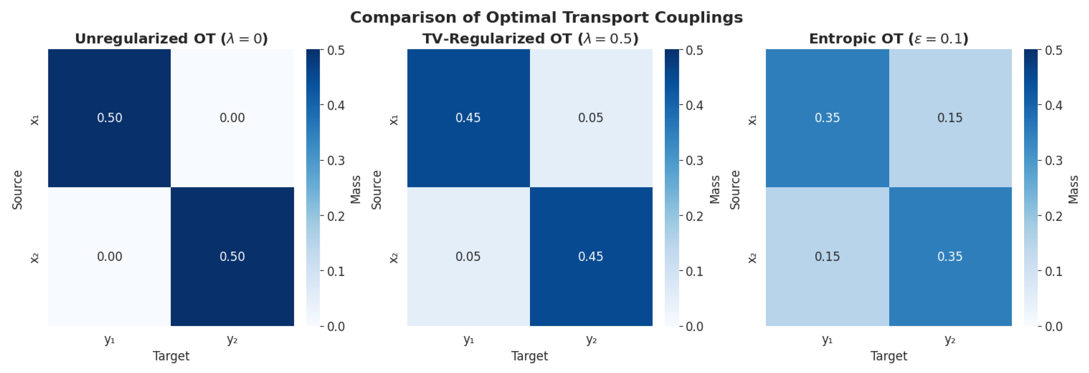
Example 10 

(Two-point distributions). Let $\mu ={\displaystyle \frac{1}{2}}{\delta }_0+{\displaystyle \frac{1}{2}}{\delta }_1$, $\nu ={\displaystyle \frac{1}{2}}{\delta }_{{\displaystyle \frac{1}{2}}}+{\displaystyle \frac{1}{2}}{\delta }_{{\displaystyle \frac{3}{2}}}$, with $d(x,y)=|x-y|$. The optimal couplings for different λ are:

• $\lambda =0$: ${\pi }_0=\left(\begin{array}{cc}{\displaystyle \frac{1}{2}}& 0\\ 0& {\displaystyle \frac{1}{2}}\end{array}\right)$, ${\mathcal{T}}_0(\mu ,\nu )={\displaystyle \frac{1}{2}}$, $D_{\mu ,\nu }\left({\pi }_0\right)=1$
• $\lambda =0.5$: ${\pi }_{0.5}=\left(\begin{array}{cc}0.45& 0.05\\ 0.05& 0.45\end{array}\right)$, ${\mathcal{T}}_{0.5}(\mu ,\nu )\approx 0.575$, $D_{\mu ,\nu }\left({\pi }_{0.5}\right)\approx 0.8$
• $\lambda \to \infty$: ${\pi }_{\infty }=\left(\begin{array}{cc}0.25& 0.25\\ 0.25& 0.25\end{array}\right)$, ${lim}_{\lambda \to \infty }{\mathcal{T}}_{\lambda }(\mu ,\nu )/\lambda =0.5$

The unregularized solution is sparse (two zeros), while entropic regularization would yield a fully dense matrix. TV regularization produces intermediate sparsity.

Example 11 

(Gaussian distributions). Consider $\mu =\mathcal{N}(0,1)$ and $\nu =\mathcal{N}(1,1)$ on $\mathbb{R}$ discretized with $n=100$ points. Figure 1 (conceptual) shows that:

• For small λ, the optimal coupling approximates the monotone rearrangement (sparse in the sense of Monge map)
• For large λ, the coupling approaches the product measure (dense but independent)
• TV regularization preserves more sparsity than entropic regularization at comparable regularization strength

9. Discussion and Future Work

We have introduced and analyzed a total variation regularized optimal transport problem. The main theoretical contributions are:

• Existence of optimal transport plans (Theorem 2)
• Proof that ${\mathcal{T}}_{\lambda }$ defines a metric for $\lambda >0$ (Corollary to Theorem 5)
• Characterization of limiting behavior as $\lambda \to 0$ and $\lambda \to \infty$ (Theorems 7 and 8)
• Discrete linear programming formulation for computation

Compared to entropic regularization, the TV-regularized formulation offers distinct advantages for applications requiring sparse couplings but comes at higher computational cost due to the linear programming structure.

Future Research Directions

• Algorithmic development: Specialized algorithms (primal-dual methods, network flow formulations, cutting-plane methods) could improve computational efficiency beyond generic LP solvers.
• Metric geometry: Study geodesics, curvature, and other geometric properties of $(\mathcal{P}\left(\mathsf{\Omega }\right),{\mathcal{T}}_{\lambda })$. Does ${\mathcal{T}}_{\lambda }$ induce a geodesic metric space?
• Statistical properties: Analyze sample complexity, consistency, and robustness of estimators based on ${\mathcal{T}}_{\lambda }$. The TV component may provide robustness to outliers.
• Applications: Explore specific domains where sparse couplings are beneficial: graph matching, feature selection, multi-marginal problems with sparsity constraints.
• Extensions: Generalize to unbalanced optimal transport (allowing mass variation), dynamic formulations (Benamou-Brenier), and other cost functions beyond $d(x,y)$.
• Hybrid approaches: Combine TV and entropic regularization to balance computational efficiency with sparsity promotion.

References

- L. V. Kantorovich. On the translocation of masses. Doklady Akademii Nauk SSSR, 37(7–8):227–229, 1942.
- C. Villani. Topics in Optimal Transportation. American Mathematical Society, 2003.
- C. Villani. Optimal Transport: Old and New. Springer, 2009.
- M. Cuturi. Sinkhorn distances: Lightspeed computation of optimal transport. In Advances in Neural Information Processing Systems, 2013.
- G. Peyré and M. Cuturi. Computational optimal transport. Foundations and Trends in Machine Learning, 11(5–6):355–607, 2019.
- L. I. Rudin, S. Osher, and E. Fatemi. Nonlinear total variation based noise removal algorithms. Physica D, 60:259–268, 1992.
- V. I. Bogachev. Measure Theory. Springer, 2007.
- A. L. Gibbs and F. E. Su. On choosing and bounding probability metrics. International Statistical Review, 70(3):419–435, 2002.
Figure 1.
Conceptual illustration: Optimal couplings for Gaussian distributions under different regularization. Left: Small (near-Monge). Center: TV regularization (). Right: Entropic regularization ().
Disclaimer/Publisher’s Note: The statements, opinions and data contained in all publications are solely those of the individual author(s) and contributor(s) and not of MDPI and/or the editor(s). MDPI and/or the editor(s) disclaim responsibility for any injury to people or property resulting from any ideas, methods, instructions or products referred to in the content. |
© 2025 by the authors. Licensee MDPI, Basel, Switzerland. This article is an open access article distributed under the terms and conditions of the Creative Commons Attribution (CC BY) license (http://creativecommons.org/licenses/by/4.0/).
Copyright: This open access article is published under a Creative Commons CC BY 4.0 license, which permit the free download, distribution, and reuse, provided that the author and preprint are cited in any reuse.